A Survey on Newhouse Thickness, Fractal Intersections and Patterns

Abstract

In this article, we introduce a notion of size for sets, called the thickness, that can be used to guarantee that two Cantor sets intersect (the Gap Lemma) and show a connection among thickness, Schmidt games and patterns. We work mostly in the real line, but we also introduce the topic in higher dimensions.

1. Newhouse’s Thickness

In the 1970s, S. Newhouse [1,2] defined the thickness of a real line. Thickness is a notion of size of a compact set, and Newhouse gave in his famous Gap Lemma a simple condition involving thickness that ensures two compact sets intersect. Since then, many mathematicians working on dynamical systems and fractal geometry have been interested in this notion of size (e.g., [3,4,5,6,7,8,9,10,11,12]).

Before giving the definition of thickness and stating the Gap Lemma, we are going to see any compact set $C\subset \mathbb{R}$ as the result of sequentially “poking holes”, starting with an interval (the convex hull of the compact set).

Let C be a compact set in $\mathbb{R}$. We denote by $I_1$ the convex hull of C. There is a sequence ${\left(G_n\right)}_n$ (that might be finite) formed by disjoint bounded open intervals that are the path-connected components of $I_1\backslash C$.

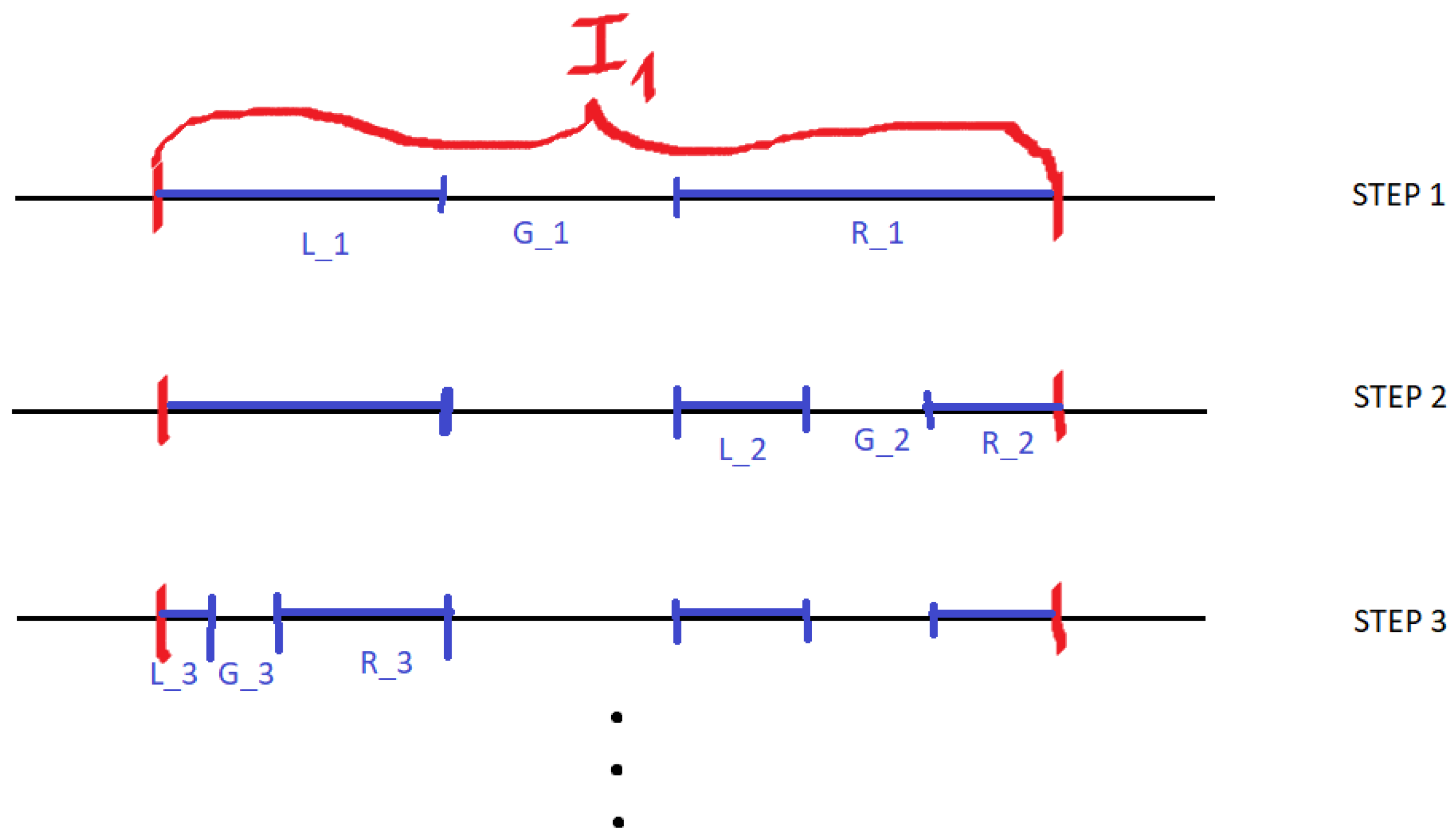
Since these intervals are disjoint and contained in the finite interval $I_1$, we can assume that they are ordered by non-increasing length. (In fact, in case there are infinitely many of them, we have ${lim}_{n\to \infty }\left|G_n\right|=0$.) If there are several intervals of the same length, then we choose any ordering by non-increasing length. We can construct the compact set C by removing these gaps in order (see Figure 1).

When we remove $G_n$ from an interval of the previous step, we obtain two new intervals $L_n$ (at the left) and $R_n$ (at the right). Note that there may be degenerate intervals (singletons).

Thickness is a notion of size that looks at the smallest proportion of lengths of intervals over the lengths of gaps:

$$\tau \left(C\right):=\underset{n}{inf}\frac{min\left\{\right|L_n|,|R_n\left|\right\}}{|G_n|}.$$

Observation 1.

When $\tau \left(C\right)\ge c$, then $\frac{|L_n|}{|G_n|}\ge c$ and $\frac{|R_n|}{|G_n|}\ge c$ for every n. Intuitively, this says that the set is large around each point of the set at every scale.

Observation 2.

In case C has at least an isolated point x, then there exists n such that $L_n=\left\{x\right\}$ or $R_n=\left\{x\right\}$, and thus $\tau \left(C\right)=0$.

Lemma 1.

Newhouse’s thickness is well-defined, where any non-increasing order for the sequence of gaps gives the same value.

Proof. 

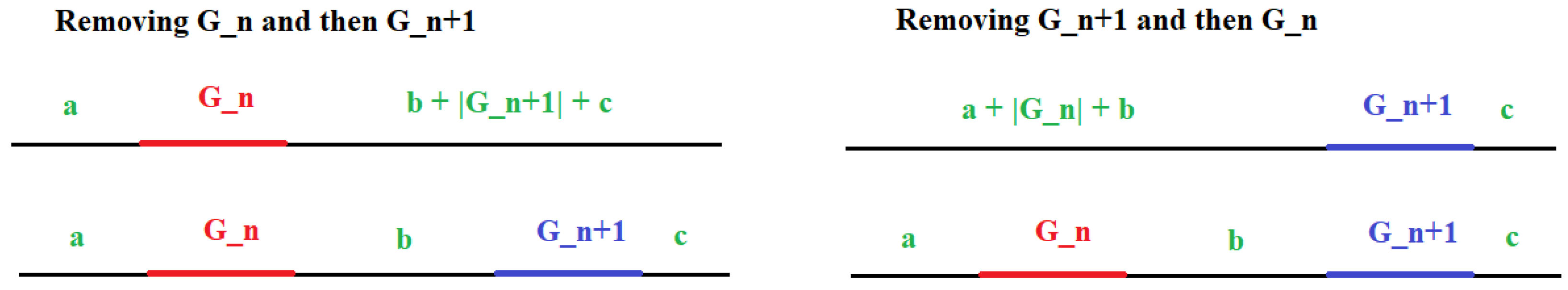
One can prove that in case there are two gaps in the sequence with the same length $g:=|G_n|=|G_{n+1}|$, switching their order in the sequence gives the same thickness. When the gaps are erased from different parents, the quotients do not change, and thus the infimum does not change. In case the gaps $G_n$ and $G_{n+1}$ are erased from the same parent, the quotients may change, but the infimum is the same when removing them in any order. Let us look at the latter case.

When we remove $G_n$ and then $G_{n+1}$ (see Figure 2), the quotients appearing in the definition of thickness are $\frac{a}{g},\frac{b+g+c}{g},\frac{b}{g}$ and $\frac{c}{g}$. When we remove $G_{n+1}$ and then $G_n$ instead (see Figure 2), the quotients appearing in the definition of thickness are $\frac{a+g+b}{g},\frac{c}{g},\frac{a}{g}$ and $\frac{b}{g}$. Note that

$$inf\{\frac{a}{g},\frac{b+g+c}{g},\frac{b}{g},\frac{c}{g}\}=inf\{\frac{a}{g},\frac{b}{g},\frac{c}{g}\}=inf\{\frac{a+g+b}{g},\frac{c}{g},\frac{a}{g},\frac{b}{g}\}.$$

Now, observe that since there are finitely many gaps with a fixed length, in finite steps, one can order all gaps with the same length as $|G_n|$ through applying permutations, as shown before.

After this, note that there is a sequence of steps ${\left(N_k\right)}_k$, where $|G_{N_k}|>|G_{N_k+1}|$ and in which the thickness does not change when we reordering gaps with the same length up to those steps. (We may reorder the first $N_k$ terms of the sequence, but the sequence tails remain the same.) We conclude that the thickness does not change: □

Observation 3.

In general, the order of the sequence of gaps matters (i.e., if we consider the sequence of gaps in an order that is not by non-increasing length, we may obtain a different result).

Observation 4.

The definition of thickness is invariant under homothetic functions, where $\tau (aC+b)=\tau \left(C\right)$ for any $a\ne 0$ because homothetic functions preserve the proportions. However, in general, the thickness is not invariant under smooth diffeomorphisms.

Example 1.

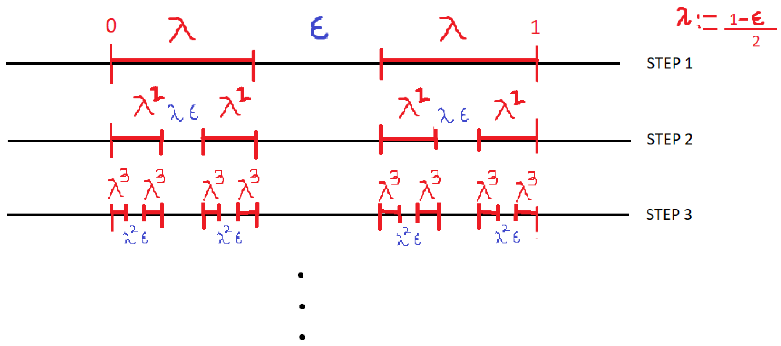
(Thickness of the central Cantor sets). Given $\epsilon \in (0,1)$, let $M_{\epsilon }$ be the middle ε Cantor set, which is obtained by starting with the interval $[0,1]$ and then iterating the process of removing from each interval in the construction the middle open interval of a relative length ε (see Figure 3).

Every time we remove a gap $G_n$ to obtain the step m of the construction, we have

$$\frac{min\left\{\right|L_n|,|R_n\left|\right\}}{|G_n|}=\frac{{\lambda }^m}{{\lambda }^{m-1}\epsilon }=\frac{\lambda }{\epsilon }=\frac{1-\epsilon }{2\epsilon }.$$

Then, we have

$$\tau \left(M_{\epsilon }\right):=\underset{n}{inf}\frac{min\left\{\right|L_n|,|R_n\left|\right\}}{|G_n|}=\frac{1-\epsilon }{2\epsilon }.$$

2. The Gap Lemma

2.1. Why Thickness and the Gap Lemma?

Newhouse’s motivation for defining thickness was the Gap Lemma, giving conditions for two compact sets in the real line to intersect. To motivate the definition of thickness and the assumptions of the Gap Lemma, we start by looking at the most basic non-trivial case: two sets where each of them is formed by a union of two closed disjoint intervals.

If the compact sets are disjoint, then we have the following possible cases:

• Their convex hulls are disjoint:

• One of the sets is contained in a gap of the other set:

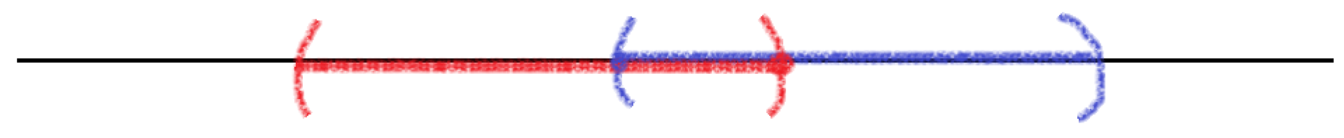
• The sets are “interleaved”, as shown below:

Let us study the first interleaved case:

We have $|L^2|<|G^1|$ and $|R^1|<|G^2|$. Hence, $\frac{|L^2\left|\right|R^1|}{|G^1\left|\right|G^2|}<1$, and therefore

$$\tau \left(C\right)\tau \left(C^{\prime }\right):=\frac{min\left\{\right|L^1|,|R^1\left|\right\}}{|G^1|}\frac{min\left\{\right|L^2|,|R^2\left|\right\}}{|G^2|}<1.$$

The same happens with the other interleaved case. Therefore, in this simple case, we obtian the following:

Lemma 2.

(Baby Gap Lemma). Let C and $C^{\prime }$ be the disjoint unions of two compact intervals. If their convex hulls intersect, then each set is not contained in a gap of the other one, and $\tau \left(C\right)\tau \left(C^{\prime }\right)\ge 1$. Then, $C\cap C^{\prime }\ne \varnothing$.

2.2. The Gap Lemma

Newhouse’s Gap Lemma (See, for example, ([1], Lemma 3.5 for a first version of it or, in general, ([2], Lemma 4. See also ([13], page 63.) is a natural generalization of Lemma 2 but now considers the general compact sets in the line. We denote the convex hull of a set C with $conv\left(C\right)$:

Theorem 1.

(Newhouse’s Gap Lemma). Let $C^1$ and $C^2$ be two compact sets in the real line such that the following are true:

1. 

$conv\left(C^1\right)\cap conv\left(C^2\right)\ne \varnothing$;

2. 

Neither set lies in a gap of the other compact set;

3. 

$\tau \left(C^1\right)\tau \left(C^2\right)\ge 1$.

Then, we have

$$C^1\cap C^2\ne \varnothing .$$

Note that if we decide to consider the unbounded path’s connected components of the complement of the compact set as “gaps”, then the second hypothesis would imply the first one. However, in this survey, we do not consider them as gaps, since their lengths do not appear in the denominator of the definition of thickness:

Observation 5 (Sharpness of Theorem 1).

Given two positive numbers${\tau }_1$and${\tau }_2$such that${\tau }_1{\tau }_2<1$, we can construct compact sets$C^1,C^2$with thicknesses${\tau }_1,{\tau }_2$, respectively, that are not contained in a gap of the other one, and their intersection is empty: Then, take

$$C^1:=[0,1]\cup [1+{\tau }_1^{-1},2+{\tau }_1^{-1}]$$

which is a compact set with a thickness${\tau }_1$. Since, by the hypothesis,${\tau }_1^{-1}>{\tau }_2>0$, there is an$\epsilon \in (0,\frac{{\tau }_1^{-1}}{2})$such that$\frac{{\tau }^{-1}-2\epsilon }{1+2\epsilon }={\tau }_2$. Define

$$C^2=[-{\tau }_1^{-1}+\epsilon ,-\epsilon ]\cup [1+\epsilon ,1+{\tau }_1^{-1}-\epsilon ]$$

which is a compact set with a thickness${\tau }_2$. It is easy to see that$C^1\cap C^2=\varnothing$, their convex hulls intersect, and none of them are contained in a gap of the other one.

In order to prove the Gap Lemma, we need to introduce two definitions:

Definition 1.

We say that two open intervals are linked if each of them contains exactly one endpoint of the other (see Figure 4).

Definition 2.

Let C be a compact set in the real line with a sequence of gaps ${\left(G_n\right)}_n$ ordered by non-increasing length. Let v be an endpoint of $G_n$. We define the bridge $B\left(v\right)$ associated with v to be $L_n$ or $R_n$, depending on whether v is the leftmost or rightmost point of $G_n$.

Proof of Theorem 1. 

We are going to prove the Gap Lemma by contradiction. Let $C^1$ and $C^2$ be compact sets satisfying the assumptions of the Gap Lemma, and assume $C^1\cap C^2=\varnothing$. Let ${\left(G_m^1\right)}_m$ and ${\left(G_n^2\right)}_n$ the sequences of gaps of the compact sets $C^1$ and $C^2$, respectively, ordered by non-increasing length.

It is enough to construct a sequence of pairs ${(G_{m_i}^1,G_{n_i}^2)}_i$ of the linked gaps of $C^1$ and $C^2$ (where we advance in n and m that $n_i<n_{i+1}$ and $m_i<m_{i+1}$). Then, by taking $x_i$ and $y_i$ to be the leftmost points of $G_{m_i}^1$ and $G_{n_i}^2$, respectively, we find that $x_i\in C^1$ and $y_i\in C^2$. By passing to subsequences, if necessary, we may assume that $x_i\to x,y_i\to y$. When observing that

$$\begin{array}{cc}\hfill dist(x,y)& =\underset{i\to \infty }{lim}dist(x_i,y_i)\le \underset{i\to \infty }{lim}diam(G_{m_i}^1\cup G_{n_i}^2)\hfill \\ \hfill & \le \underset{i\to \infty }{lim}diam\left(G_{m_i}^1\right)+diam\left(G_{n_i}^2\right)=0,\hfill \end{array}$$

we then find that $x=y\in C^1\cap C^2$, which is a contradiction.

We will construct the sequence of pairs of linked gaps by induction. To begin, observe the following:

• Any endpoint of the convex hull of $C^i$ or a gap of $C^i$ belongs to $C^i$.
• If a point belongs to $conv\left(C^i\right)$ but does not belong to $C^i$, then it is in a gap $G_m^i$.
• If a point belongs to $C^i$, then (by the assumption $C^1\cap C^2=\varnothing$) the point is either outside of $conv\left(C^j\right)$ ($j:=3-i$) or in a gap $G_n^j$.

In order to be able to handle the inductive step, we will prove a slightly stronger statement: there is a sequence of pairs of gaps $G_{m_i}^1$ and $G_{n_i}^2$ that are linked such that there is an endpoint of one, and thus its bridge is contained in the other gap.

First step. By the first assumption (Equation (1)) and symmetry, we may assume that there is an endpoint of $conv\left(C^2\right)$ that belongs to $conv\left(C^1\right)$, and thus it is in $C^2\cap conv\left(C^1\right)$. However, since $C^1\cap C^2=\varnothing$, then it belongs to $G_{m_1}^1\cap C^2$ for some gap $G_{m_1}^1$. Thus, we have

$$G_{m_1}^1\cap C^2\ne \varnothing .$$

(1)

Since the endpoints of $G_{m_1}^1$ belong to $C^1$, each of them must be either outside of $conv\left(C^2\right)$ or in a gap of $C^2$. Since, by construction, $G_{m_1}^1$ contains an endpoint of $conv\left(C^2\right)$, one of them is outside $conv\left(C^2\right)$. The other one must belong to $conv\left(C^2\right)$ (and therefore to a gap of $C^2$), because otherwise, $C^2\subseteq G_{m_1}^1$, contradicting the assumption in Equation (2).

We have seen that there is an endpoint of $G_{m_1}^1$ in a gap $G_{n_1}^2$, and there is an endpoint of $G_{m_1}^1$ outside $conv\left(C^2\right)$. This implies that there is an endpoint $v_{n_1}^2$ of $G_{n_1}^2$ such that $B\left(v_{n_1}^2\right)\subseteq G_{m_1}^1$ (in particular, $G_{m_1}^1$ and $G_{n_1}^2$ are linked). This is the starting point of the induction.

The inductive step. Assume that $G_{m_i}^1$ and $G_{n_i}^2$ are linked gaps, where $B\left(v_{n_i}^2\right)\subseteq G_{m_i}^1$ and $v_{n_i}^2$ is an endpoint of $G_{n_i}^2$ (the symmetric condition is identical). Let $u_{m_i}^1$ be the endpoint of $G_{m_i}^1$ that is in $G_{n_i}^2$.

Let us see that $B\left(u_{m_i}^1\right)$ cannot be contained in $G_{n_i}^2$. Otherwise, since $B\left(u_{m_i}^1\right)\subseteq G_{n_i}^2$ and $B\left(v_{n_i}^2\right)\subseteq G_{m_i}^1$, we would have

$$\tau \left(C^1\right)\tau \left(C^2\right)\le \frac{\left|B\right(u_{m_i}^1\left)\right|}{|G_{m_i}^1|}\frac{\left|B\right(v_{n_i}^2\left)\right|}{|G_{n_i}^2|}<1,$$

which contradicts the thickness assumption in Equation (3).

Then, the other endpoint $u_{n_i}^2$ of $G_{n_i}^2$ belongs to $B\left(u_{m_i}^1\right)$, and thus $u_{n_i}^2\in C^2\cap B\left(u_{m_i}^1\right)\subseteq {\left(C^1\right)}^C\cap B\left(u_{m_i}^1\right)$. Therefore, $u_{n_i}^2\in G_{m_{i+1}}^1$ with $m_{i+1}>m_i$.

Then, by taking $G_{n_{i+1}}^2:=G_{n_i}^2$ and $G_{m_{i+1}}^1$ as above, we find linked gaps with a bridge of an endpoint of $G_{m_{i+1}}^1$ contained in $G_{n_i}^2$ (because the bridge is contained between $G_{m_i}^1$ and $G_{m_{i+1}}^1$). □

3. Connection to the Hausdorff Dimension

Thickness is a notion of the size of a set. The Hausdorff dimension is another more classical notion of size. They are different but related. In this section, we explore the connections between these concepts.

We begin by recalling the definition of the Hausdorff dimension (for a more complete background on the Hausdorff dimension, see [14,15,16]):

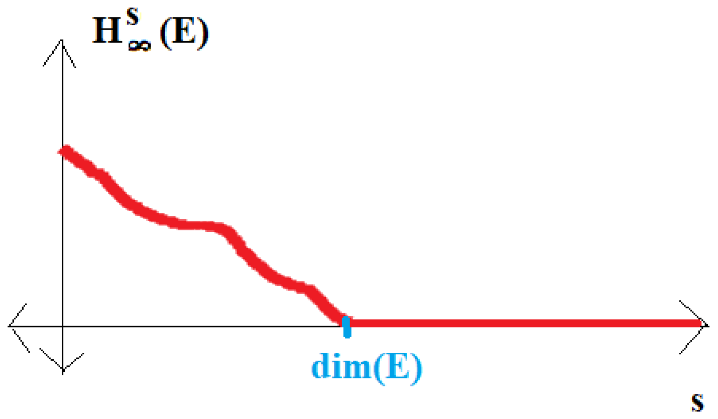
Definition 3.

The s-dimensional Hausdorff content of E is

$$H_{\infty }^s\left(E\right):=inf\left\{\sum _{k\in \mathbb{N}}diam{\left(U_k\right)}^s:E\subseteq \bigcup _{k\in \mathbb{N}}{U}_k\mathit{and}{\left\{U_k\right\}}_k\mathit{is}a\mathit{family}\mathit{of}\mathit{open}\mathit{sets}\right\}.$$

The Hausdorff dimension of E is the supremum of all real-valued s, for which the s-dimensional Hausdorff content of E is positive (see Figure 5).

The following result shows that sets of large thicknesses also have large Hausdorff dimensions:

Theorem 2.

By letting $C\subset \mathbb{R}$ be a compact set with a thickness $\tau \left(C\right)>0$, then

$${dim}_H\left(C\right)\ge \frac{log\left(2\right)}{log(2+\frac{1}{\tau \left(C\right)})}.$$

In particular, ${dim}_H\left(C\right)\to 1$ as $\tau \left(C\right)\to \infty$.

Observation 6 (Sharpness of Theorem 2).

Given $\tau \in (0,\infty )$, we can take $C:=M_{\epsilon }\subseteq \mathbb{R}$ to be the middle Cantor set with a relative gap length $\epsilon :=\epsilon \left(\tau \right):=\frac{1}{2\tau +1}$. Then, the relative length of each child in its parent is $\alpha :=\frac{\tau }{1+2\tau }$. Through Example 1, we have $\tau \left(C\right)=\frac{1-\epsilon }{2\epsilon }=\tau$, and through [16] (Example 4.4) (taking $m=2$), we have ${dim}_H\left(C\right)=\frac{log\left(2\right)}{log\left({\alpha }^{-1}\right)}=\frac{log\left(2\right)}{log(2+\frac{1}{\tau })}$.

Observation 7.

Theorem 2 shows that sets with large thicknesses have large Hausdorff dimensions. The converse does not hold. In fact, there are sets of positive Lebesgue measures (which imply full Hausdorff dimensions) with thicknesses of 0. Consider, for example, the union of a closed interval with an isolated point.

Proof of Theorem 2.

We define

$$\beta :=\frac{log\left(2\right)}{log(2+\frac{1}{\tau \left(C\right)})}.$$

This is enough to prove that for any $\mathcal{U}:={\left\{U_i\right\}}_i$ open covering of C, we have ${\sum }_i|U_i{|}^{\beta }\ge {|conv\left(C\right)|}^{\beta }>0$.

Fix $\mathcal{U}:={\left\{U_i\right\}}_i$ to an open covering of C. Since $C\subseteq \mathbb{R}$ is a compact set, and the sum decreases while dropping elements of the sequence of $\mathcal{U}$, we can assume that the covering $\mathcal{U}$ is formed by finitely many elements.

The case in which $\mathcal{U}$ is formed by an interval U is trivial (because $conv\left(C\right)\subseteq U$ implies ${|conv\left(C\right)|}^{\beta }\le {\left|U\right|}^{\beta }$). Let us assume that we have at least two open intervals in $\mathcal{U}$ and reduce inductively this case to the former case.

As before, we define ${\left(G_n\right)}_n$ as the sequence of gaps in the definition of $\tau \left(C\right)$, and $L_n$ and $R_n$ are the left and right intervals associated with $G_n$, respectively.

Since $\mathcal{U}$ is a covering of C with finitely many open sets, then the convex hull of C, except for a few gaps, is covered by $\mathcal{U}$ (i.e., there exist $N\in \mathbb{N}$ and gaps $G_{m_1},\cdots ,G_{m_N}$ with $|G_{m_1}|\ge \cdots \ge |G_{m_N}|$), where

$$conv\left(C\right)\backslash \bigcup _{1\le j\le N}{G}_{m_j}\subseteq \bigcup _i{U}_i\mathrm{and}{G}_{m_j}⊈\bigcup _i{U}_i.$$

We have $L_{m_N}$ and $R_{m_N}$ as the left and right intervals associated with $G_{m_N}$, respectively, which is the smallest gap that is not covered. Then, there exist $U\left(L\right)$ and $U\left(R\right)$ in $\mathcal{U}$ such that $L_{m_N}\subseteq U\left(L\right)$ and $R_{m_N}\subseteq U\left(R\right)$.

We define $A:=conv\left(U\right(L)\cup U(R\left)\right)$. By using $L_{m_N}\subseteq U\left(L\right)$, the definition of $\tau \left(C\right)$ and the definition of A, we obtain

$$\left|U\left(L\right)\right|\ge |L_{m_N}|\ge \tau |G_{m_N}|\ge \tau (\left|A\right|-\left|U\left(L\right)\right|-\left|U\left(R\right)\right|).$$

(2)

Analogously, by using that $R_{m_N}\subseteq U\left(R\right)$, the definition of $\tau \left(C\right)$ and the definition of A, we obtain

$$\left|U\left(R\right)\right|\ge |R_{m_N}|\ge \tau |G_{m_N}|\ge \tau (\left|A\right|-\left|U\left(L\right)\right|-\left|U\left(R\right)\right|).$$

(3)

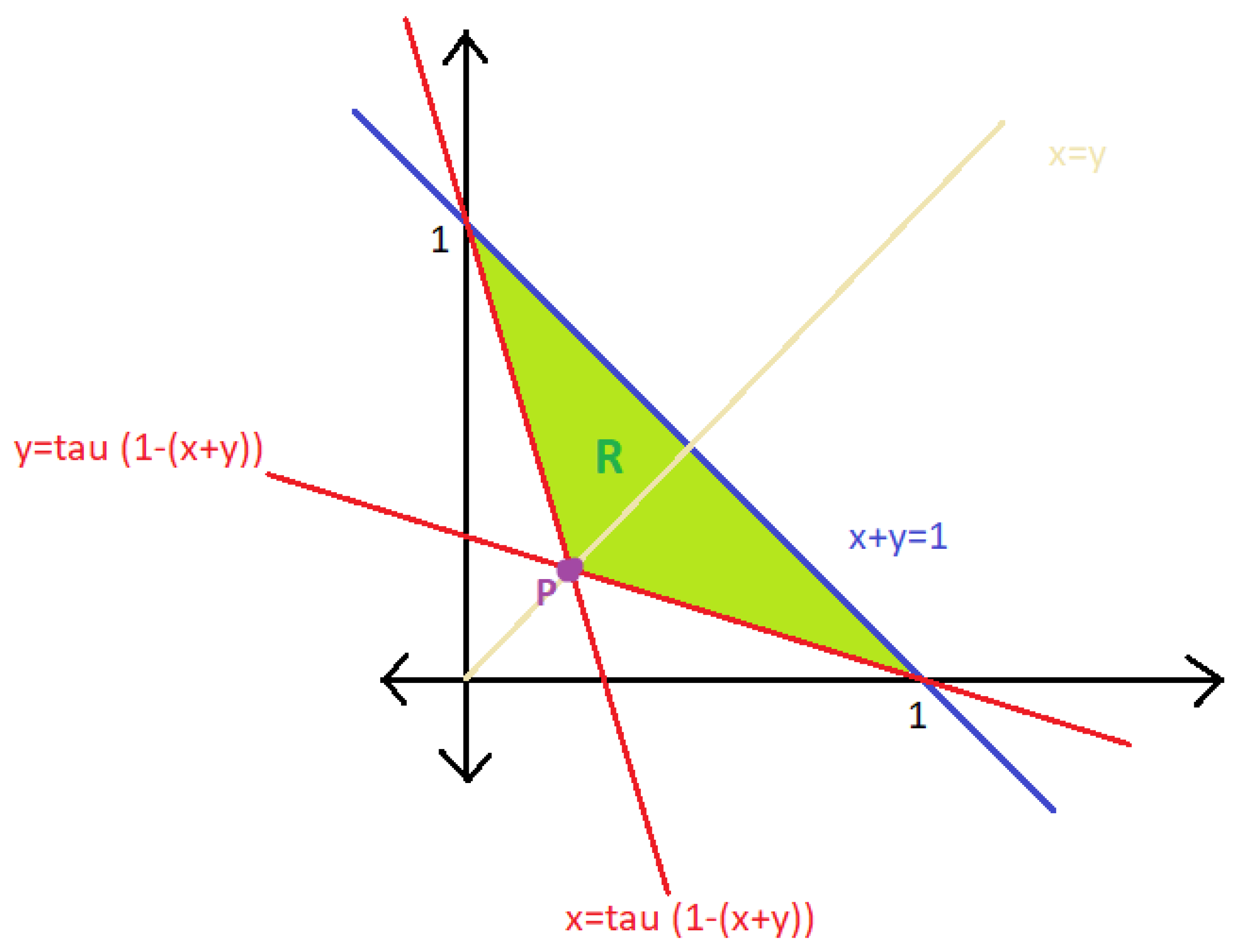
We define $x:=\frac{\left|U\right(L\left)\right|}{\left|A\right|}$ and $y:=\frac{\left|U\right(R\left)\right|}{\left|A\right|}$. The proportions x and y satisfy the following:

• $x\ge 0$ and $y\ge 0$;
• $x+y\le 1$ (because $U\left(L\right)⊍U\left(R\right)\subseteq A$);
• $\tau (1-x-y)\le x$ and, symmetrically, $\tau (1-x-y)\le y$ (because of Equations (2) and (3)).

Based on this, we define the region R by

$$R:=\{(x,y)\in {\mathbb{R}}^2:x\ge 0,y\ge 0,x+y\le 1,x\ge \tau (1-(x+y)),y\ge \tau (1-(x+y))\}.$$

The intersection of the lines $x=\tau (1-(x+y\left)\right)$ and $y=\tau (1-(x+y\left)\right)$ is the point $P=\left(\frac{1}{2+\frac{1}{\tau }},\frac{1}{2+\frac{1}{\tau }}\right)$ (see Figure 6).

Claim:

$$1=min\{x^{\beta }+y^{\beta }:(x,y)\in R\}.$$

This is a standard calculation, but we provide the details. Let $g(x,y):=x^{\beta }+y^{\beta }$. Observe that since g is increasing in x and y, the minimum is reached on the red sides of the boundary of R in Figure 6. By symmetry, it is enough to study just one red side. We want to find the minimum of g under the condition $y=1-(1+\frac{1}{\tau })x$ with $0\le x\le \frac{1}{2+\frac{1}{\tau }}$. This is the minimum of $h\left(x\right)=x^{\beta }+{\left(1-(1+\frac{1}{\tau })x\right)}^{\beta }$ with $0\le x\le \frac{1}{2+\frac{1}{\tau }}$. A calculation shows that the only critical point of $h^{\prime }$ is a maximum, so the minimum is attained at some endpoint.

We have $h\left(0\right)=1$ and $h\left(\frac{1}{2+\frac{1}{\tau }}\right)=2{\left(\frac{1}{2+\frac{1}{\tau }}\right)}^{\beta }=1$ (where the last equality holds by definition of $\beta :=\frac{log\left(2\right)}{log(2+\frac{1}{\tau \left(C\right)})}$). This gives the claim.

By applying the claim to $x:=\frac{\left|U\right(L\left)\right|}{\left|A\right|}$ and $y:=\frac{\left|U\right(R\left)\right|}{\left|A\right|}$, we find

$${\left|U\left(L\right)\right|}^{\beta }+{\left|U\left(R\right)\right|}^{\beta }\ge {\left|A\right|}^{\beta }.$$

This means that changing $U\left(L\right)$ and $U\left(R\right)$ by A in the covering $\mathcal{U}$ gives a new covering ${\mathcal{U}}^{\prime }$ with one less element by the disjoint open sets, with a smaller sum ${\sum }_i{\left|U_i^{\prime }\right|}^{\beta }$. By repeating this process, we find that ${\sum }_i|U_i{|}^{\beta }\ge {\sum }_i|U_i^{\prime }{|}^{\beta }\ge \cdots \ge {|conv\left(C\right)|}^{\beta }$. □

Observation 8.

Intuitively, the thickness looks at the smallest part of the set, while the Hausdorff dimension looks at the largest part (for example, if $C={\bigcup }_{k\in \mathbb{N}}{C}_k$, then ${dim}_H\left(C\right)={sup}_{k\in \mathbb{N}}{dim}_H\left(C_k\right)$). Therefore, it is reasonable to apply Theorem 2 to compact subsets of C. More precisely, we can define the upper thickness of a set C as $\tilde{\tau }\left(C\right):={sup}_{A\mathrm{compact}\subseteq C}\tau \left(A\right)$. Then, of course, Theorem 2 gives the same bound, replacing $\tau \left(C\right)$ by $\tilde{\tau }\left(C\right)$.

As a simple instance of this, if a set has isolated points, then the thickness is zero, while the upper thickness “gets rid” of them and can take any value.

The upper thickness in usually larger than the thickness, but in some cases, they may be equal.

4. Thickness and Patterns in Fractals

In this section, we investigate the connection between the thickness and patterns in sparse sets:

Definition 4.

We say that a set $C\subseteq {\mathbb{R}}^d$ contains a homothetic copy of P if there exist $a\in \mathbb{R}\backslash \left\{0\right\}$ and $b\in {\mathbb{R}}^d$ such that $aP+b\subseteq C$.

For example, an arithmetic progression of a length N in the real line is a homothetic copy of $\{1,\cdots ,N\}$.

The following result is well known:

Lemma 3.

Any set $C\subseteq {\mathbb{R}}^d$ of positive Lebesgue measures contains homothetic copies of every finite set.

Proof. 

Let $P=\{a_1,\cdots ,a_N\}$ be a finite set and $R:={max}_{1\le i\le N}\parallel a_i\parallel$.

We know by the Lebesgue Density Theorem that almost every point $x\in C$ satisfies

$$\underset{r\to 0}{lim}\frac{{\mathcal{L}}^d(C\cap Q_r\left(x\right))}{{\mathcal{L}}^d\left(Q_r\right)}=1$$

where $Q_r\left(x\right)$ is the cube with a center x and radius r. We fix a value of x satisfying this. Then, there exists $r_0$ such that $\frac{{\mathcal{L}}^d(C\cap Q_{r_0}\left(x\right))}{{\mathcal{L}}^d\left(Q_{r_0}\right)}>1-\frac{1}{10N}$.

By rescaling and translating the set C and the cube $Q_{r_0}\left(x\right)$, we can assume $Q_{r_0}\left(x\right)={[0,1]}^d$. Then, we know that ${\mathcal{L}}^d(C\cap {[0,1]}^d)>1-\frac{1}{10N}$.

This is enough to prove that

$${\mathcal{L}}^d\left(\bigcap _{1\le i\le N}(C-\frac{a_i}{10RdN})\right)>0.$$

Then, in particular, ${\bigcap }_{1\le i\le N}(C-\frac{a_i}{10RdN})$ is non-empty, and any point y in the intersection satisfies

$$y+{\left(10RdN\right)}^{-1}P\subset C.$$

Note that if $B\subseteq {[0,1]}^d$ and ${\parallel v\parallel }_2\le r$, then ${\mathcal{L}}^d\left((B-v)\cap {[0,1]}^d\right)\ge {\mathcal{L}}^d\left(B\right)-dr$. By applying this to $B:=C\cap {[0,1]}^d$ and $v_i:=\frac{a_i}{10RdN}$ whose norm is smaller than $r:=\frac{1}{10dN}$, we obtain

$$\begin{array}{cc}\hfill {\mathcal{L}}^d\left((C\cap {[0,1]}^d-\frac{a_i}{10RdN})\cap {[0,1]}^d\right)& \ge {\mathcal{L}}^d(C\cap {[0,1]}^d)-\frac{1}{10N}\hfill \\ & \ge 1-\frac{2}{10N}.\hfill \end{array}$$

If $A_1$, ⋯, $A_N\subseteq {[0,1]}^d$ satisfy ${\mathcal{L}}^d\left(A_i\right)\ge 1-{\epsilon }_i$ for all i, then

$${\mathcal{L}}^d\left(\bigcap _{1\le i\le N}{A}_i\right)\ge 1-\sum _{1\le i\le N}{\epsilon }_i.$$

We apply this to $A_i:=(C\cap {[0,1]}^d-\frac{a_i}{10RdN})\cap {[0,1]}^d$ and ${\epsilon }_i=\frac{2}{10N}$ to obtain

$$\begin{array}{cc}\hfill {\mathcal{L}}^d\left(\bigcap _{1\le i\le N}(C-\frac{a_i}{10RdN})\right)& \ge {\mathcal{L}}^d\left(\bigcap _{1\le i\le N}{A}_i\right)\hfill \\ \hfill & \ge 1-\sum _{1\le i\le N}\frac{2}{10N}=1-\frac{1}{5}>0.\hfill \end{array}$$

□

Since a positive Lebesgue measure guarantees homothetic copies of every finite set, it is natural to ask whether a weaker notion of size guarantees copies too. A natural notion of size to consider is the Hausdorff dimension. However, Keleti [17] proved that there exists a compact set $C\subseteq \mathbb{R}$, with a full Hausdorff dimension one, which does not contain any arithmetic progression of a length of three. Afterward, Keleti [18] improved this by constructing full Hausdorff dimensional compact sets in the real line, avoiding homothetic copies of triplets in any given countable collection. Maga [19] generalized this result to the complex plane. Máthé [20] constructed large Hausdorff dimensional compact sets avoiding polynomial patterns. In particular, he generalized Keleti’s result to a countable amount of many linear patterns. Finally, Yavicoli [21] studied what happens “in between” a positive Lebesgue measure and Hausdorff dimension one by considering a more general notion of Hausdorff measures.

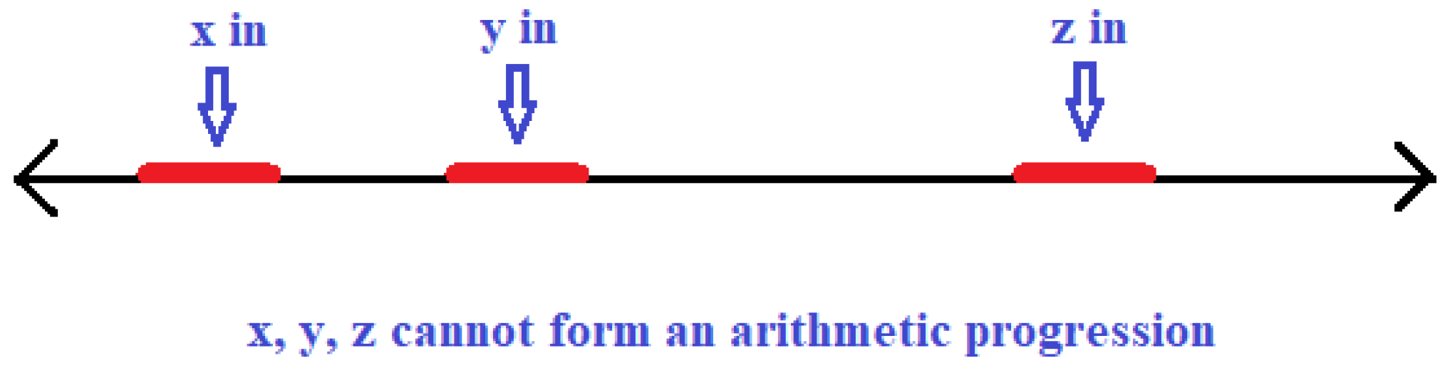
These facts indicate that Hausdorff measures and Hausdorff dimensions cannot by themselves detect the presence or absence of patterns in sets of a Lebesgue measure of zero, even in the most basic case of arithmetic progressions. Thus, it is natural to seek a different notion of size that is able to detect patterns in sets of zero Lebesgue measures.

One of the ideas behind Keleti’s construction is avoiding the given proportion everywhere at some scales of the construction (see Figure 7). This picture happens on a “zero density” set of scales. Thus, the Hausdorff dimension can still be large (at “almost all” scales, the set is large). The notion of thickness is useful to avoid such examples. Even one scale that looks like the one in Figure 7 makes the thickness small.

Before studying the patterns in arelationship with thick sets, let us mention that the Hausdorff dimension can be useful to detect some nonlinear patterns (see [22]) or to detect the arithmetic progressions of a length of three, assuming additional Fourier decay hypotheses, which are often not explicit or hard to check (see [23,24,25]). This suggests that it is natural to try to find explicit checkable conditions on a compact set that ensure that it contains arithmetic progressions, as well as other patterns.

Before studying arithmetic progressions, let us consider a different pattern—distances—using Newhouse’s thickness and the Gap Lemma. We define the set of distances of a set $C\subseteq \mathbb{R}$ as

$$\Delta \left(C\right):=\left\{\right|y-x|:x,y\in C\}.$$

Lemma 4.

Let $C\subseteq \mathbb{R}$ be a compact set with $conv\left(C\right)=[0,1]$ and $\tau \left(C\right)\ge 1$. Then, $\Delta \left(C\right)=[0,1]$.

Proof. 

We know that $\Delta \left(C\right)\subseteq [0,1]$, $0\in \Delta \left(C\right)$ because $C\ne \varnothing$ and $1\in \Delta \left(C\right)$ because $0,1\in C$. It remains to be seen whether any $t\in (0,1)$ belongs to $\Delta \left(C\right)$.

The sets C and $C-t$ satisfy the hypotheses of the Gap Lemma. Since $conv\left(C\right)=[0,1]$ and $conv(C-t)=[-t,1-t]$, the convex hulls of C and $C-t$ intersect, and each set cannot be contained in a gap of the other set. Finally, using $\tau \left(C\right)\ge 1$ and the invariance of the thickness under translation, we obtain $\tau \left(C\right)\tau (C-t)=\tau {\left(C\right)}^2\ge 1$. By the Gap Lemma, there is $x\in C\cap (C-t)$, and thus $t=(x+t)-x\in C-C$ (which means that $t\in \Delta \left(C\right)$ because $t>0$). □

Now, we are going to see that, unlike the Hausdorff dimension, the set of large thicknesses contains three-term progressions:

Proposition 1.

Let $C\subseteq \mathbb{R}$ be a compact set with $\tau \left(C\right)\ge 1$. Then, C contains an arithmetic progression of a length of three.

Proof. 

Since the thickness of the compact set and arithmetic progression are invariant under homothetic functions, we can assume that $conv\left(C\right)=[0,1]$.

This is the idea: if we prove that $C\cap \frac{C+C}{2}\ne \varnothing$, then there are $a,b,c\in C$ such that $c=\frac{a+b}{2}$. Then, $\{a,\frac{a+b}{2},b\}\subseteq C$. The problem is that a priori, we could have $a=b$. To avoid this issue we, are going to consider two disjoint subsets of C (A and B below) and prove that $C\cap \frac{A+B}{2}\ne \varnothing$.

Let $G:=(a_1,a_2)$ be the longest gap of C. Since $\tau \left(C\right)>0$, then $0<a_1<a_2<1$. The set $[0,1]\backslash G$ consists of two intervals: $L=[0,a_1]$ and $R=[a_2,1]$. We can assume that

$$a_1\le 1-a_2,$$

Otherwise, we would work with $-C+2$ instead.

Let $A:=C\cap [0,a_1]$ and $B:=C\cap [a_2,1]$. Since we want to show that $C\cap \frac{A+B}{2}\ne \varnothing$, we want to understand $A+B$.

Claim: $A+B=[a_2,1+a_1]$

Clearly, $A+B\subseteq [0,a_1]+[a_2,1]=[a_2,1+a_1]$, and so we need to see the other inclusion. We have that

$$|conv(-A)|=|conv\left(A\right)|=a_1$$

and

$$\tau (-A)=\tau \left(A\right)=\tau (C\cap [0,a_1])\ge \tau \left(C\right)\ge 1.$$

Observe that $\tau (C\cap [0,a_1])\ge \tau \left(C\right)$ holds because $G_1$ is the largest gap (otherwise, this may not be true since, in general, the thickness is not well behaved with respect to intersections).

Analogously with $B-t$, we have

$$|conv(B-t)|=1-a_2\mathrm{and}\tau (B-t)\ge 1.$$

We are going to apply the Gap Lemma to $-A$ and $B-t$ for any $t\in [a_2,1+a_1]$. Let us see whether the assumptions are satisfied.

Note that

$$\begin{array}{cc}\hfill & conv(-A)\cap conv(B-t)\ne \varnothing \hfill \\ \hfill & \iff \exists \mathrm{an}\mathrm{endpoint}\mathrm{of}-A\mathrm{between}\mathrm{the}\mathrm{endpoints}\mathrm{of}B-t\hfill \\ \hfill & \iff -a_1\in [a_2-t,1-t]\mathrm{or}0\in [a_2-t,1-t]\hfill \\ \hfill & \iff t\in [a_1+a_2,1+a_1]\mathrm{or}t\in [a_2,1]\hfill \\ \hfill & \iff t\in [a_2,1+a_1],\hfill \end{array}$$

where the last equivalence holds, since we assume $a_1+a_2\le 1$.

Then, we have the following:

• $-A$ is not contained in a gap of $B-t$. This is true because, since $\tau \left(C\right)\ge 1$, $|conv(-A\left)\right|$$\ge \left|G\right|\ge |\mathrm{any}\mathrm{gap}\mathrm{of}B-t|$. Analogously, $B-t$ is not contained in a gap of A.
• $conv(-A)\cap conv(B-t)\ne \varnothing$, since we are considering values of $t\in [a_2,1+a_1]$.
• $\tau (-A)\tau (B-t)\ge 1$.

Then, the Gap Lemma yields that for all $t\in [a_2,1+a_1]$, there is $x_t\in (-A)\cap (B-t)$, and then $t=(-x_t)+(x_t+t)\in A+B$, giving the claim.

Claim: $C\cap \frac{A+B}{2}\ne \varnothing$

We are going to prove that, in fact, $a_2\in \frac{A+B}{2}$ (note that $a_2\in C$).

Since $A+B=[a_2,1+a_1]$, we know that

$$a_2\in \frac{A+B}{2}\iff a_2\le \frac{1+a_1}{2}.$$

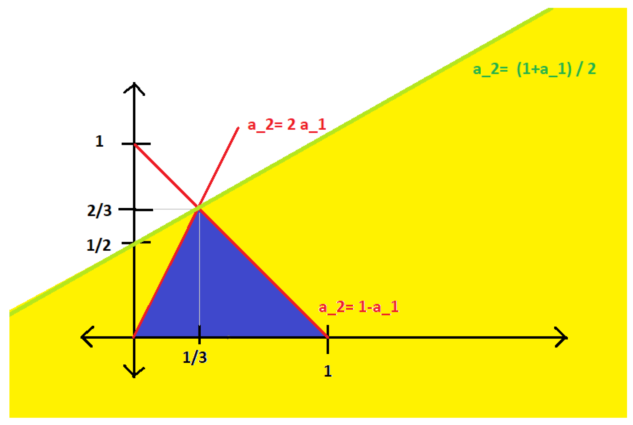
Where are the pairs $(a_1,a_2)$ that we are working with?

• We have $a_1=|conv\left(A\right)|\ge \left|G\right|=a_2-a_1$ such that $2a_1\ge a_2$.
• We are assuming that $a_1\le 1-a_2$.
• $0<a_1<a_2<1$.

As we can see in Figure 8, the blue region of pairs $(a_1,a_2)$ is contained in the yellow region $\{a_2\le \frac{1+a_1}{2}\}$. In particular, we must have $a_2\le \frac{1+a_1}{2}$ so that $a_2\in \frac{A+B}{2}$, as claimed.

We have seen that C contains an arithmetic progression $\{a,(a+b)/2,b\}$. This is indeed a non-degenerate progression since $a\in A,b\in B$ and A and B are disjoint, so the proof is complete. □

What about longer arithmetic progressions? For example, what is the length of the longest arithmetic progression that is contained in the middle $\epsilon$ Cantor set?

Lemma 5.

The middle ε Cantor set $M_{\epsilon }$ does not contain an arithmetic progression of a length $\lfloor \frac{1}{\epsilon }\rfloor +2$.

Proof. 

Take $\lambda :=\frac{1-\epsilon }{2}$. The length of any interval of step k of the construction is ${\lambda }^k$ (for $k\ge 0$), and the length of any gap of the step k of the construction is ${\lambda }^{k-1}\epsilon$ (for $k\ge 1$). Assume that there is an arithmetic progression $a+\Delta j$, $j=1,\dots ,N$ (with $\Delta >0$) contained in $M_{\epsilon }$. Then, by self-similarity, there is a first step $k\in \mathbb{N}\cup \left\{0\right\}$ such that the arithmetic progression is contained in an interval of step k but splits in step $k+1$. Hence, $|(a+\Delta N)-(a+\Delta )|=\Delta (N-1)\le {\lambda }^k$ and $\Delta \ge {\lambda }^k\epsilon$. Therefore, ${\lambda }^k\ge {\lambda }^k\epsilon (N-1)$, and thus $\frac{1}{\epsilon }+1\ge N$. □

Finding the lower bounds for the length of the longest arithmetic progression in $M_{\epsilon }$ is more difficult. Broderick, Fishman and Simmons [26] proved the following result:

Theorem 3 (Broderick, Fishman and Simmons).

For when $\epsilon >0$ sufficiently small, the $M_{\epsilon }$ middle ε Cantor set contains an arithmethic progression of a length $c\frac{\frac{1}{\epsilon }}{log\left(\frac{1}{\epsilon }\right)}$, where c is a very small constant.

By the two previous results, we know that for $\epsilon >0$ to be sufficiently small, then

$$\frac{\frac{1}{\epsilon }}{log\left(\frac{1}{\epsilon }\right)}\lesssim \mathrm{longest}\mathrm{AP}\mathrm{contained}\mathrm{in}{M}_{\epsilon }\lesssim \frac{1}{\epsilon }.$$

The precise asymptotic behavior remains an open problem.

We will not give a proof of Theorem 3. The very rough idea behind the proof is as follows:

$$\begin{array}{cc}\hfill & C\mathrm{contains}\mathrm{an}\mathrm{arithmetic}\mathrm{progression}\mathrm{of}\mathrm{length}n\mathrm{and}\mathrm{gap}\mathrm{length}\lambda \hfill \\ \hfill & \iff \mathrm{there}\mathrm{is}x\mathrm{so}\mathrm{that}x+k\lambda \in C\forall 1\le k\le n\hfill \\ \hfill & \iff \bigcap _{1\le k\le n}(C-k\lambda )\ne \varnothing \hfill \end{array}$$

Then, the existence of arithmetic progressions of a length n is reduced to proving that intersections of certain n sets are non-empty. Unfortunately, the Gap Lemma does not generalize in any simple way to intersections of three or more sets, and for this reason, the authors use a different approach: the potential game, which is a game of the Schmidt type.

The classical Schmidt game was defined in 1966 by Wolfgang Schmidt to study badly approximable numbers, and since then, many variants of the original game have been developed, mainly to study problems in diophantine approximation.

As a general idea, the potential game is a game in which there are certain rules and two players: Bob, who decides where we are going to zoom in, and Alice, who decides what to erase there. Bob has limits on how far to zoom in, and Alice has limits on how much to erase. There are also special sets called winning sets, which are subsets of the “board game”. A set W is winning if Alice has a strategy guaranteeing that if she does not erase the limit point of convergence for Bob’s moves during the game, then that point belongs to W. Being a winning set (for certain parameters) can be considered another notion of a “large size” for the set.

Broderick, Fishman and Simmons showed that a slight modification of a middle $\epsilon$ Cantor set is a winning set with certain parameters. Then, they used the intersections of the winning sets (for certain other parameters) and found a result that gave a (positive) lower bound for the Hausdorff dimension of a winning set inside certain balls. In particular, the intersection was non-empty.

As a remark, winning sets for the classical Schmidt’s game and many variants have a full Hausdorff dimension. This is not the case for the potential game (with fixed parameters). This makes it useful for studying fractal sets that do not have a full Hausdorff dimension.

We will define now the potential game in a restricted context (on the real line, where Alice is able to erase neighborhoods of points and the game can be extended to higher dimensions and more general sets).

Definition 5 (Potential game in $\mathbb{R}$).

Given $\alpha ,\beta ,\rho >0$ and $c\ge 0$, Alice and Bob play the $(\alpha ,\beta ,c,\rho )$ potential game in ${\mathbb{R}}^d$ under the following rules:

• For each $m\in {\mathbb{N}}_0$, Bob plays first, and then Alice plays.
• On the mth turn, Bob plays a closed ball $B_m:=B[x_m,{\rho }_m]$. The first ball must satisfy ${\rho }_0\ge \rho$. The following moves must satisfy ${\rho }_m\ge \beta {\rho }_{m-1}$ and $B_m\subseteq B_{m-1}$ for every $m\in \mathbb{N}$.
• On the mth turn, Alice responds by choosing and erasing a finite or countably infinite collection ${\mathcal{A}}_m={\left\{A_{{\rho }_{i,m}}\right\}}_i$ of balls with radii ${\rho }_{i,m}>0$. Alice’s collection must satisfy the following:

  $$\begin{array}{cc}\hfill \sum _i{\rho }_{i,m}^c\le {\left(\alpha {\rho }_m\right)}^c& \mathit{if}c>0\hfill \\ \hfill {\rho }_{1,m}\le \alpha {\rho }_m& \mathit{if}c=0(\mathit{in}\mathit{this}\mathit{case},\mathit{Alice}\mathit{can}\mathit{erase}\mathit{just}\mathit{one}\mathit{set}).\hfill \end{array}$$
• Alice is not allowed to erase any set or, equivalently, to pass her turn.
• Bob must ensure that ${lim}_{m\to \infty }{\rho }_m=0$.

There exists a single point

$$\left\{x_{\infty }\right\}=\bigcap _{m\in {\mathbb{N}}_0}{B}_m$$

called the outcome of the game.

We say a set $S\subset {\mathbb{R}}^d$ is an $(\alpha ,\beta ,c,\rho )$-winning set if Alice has a strategy guaranteeing that

$$\mathrm{if}{x}_{\infty }\notin \bigcup _{m\in {\mathbb{N}}_0}\bigcup _i{A}_{{\rho }_{i,m}}\mathit{then}{x}_{\infty }\in S.$$

The potential game has several elementary but very useful properties:

Lemma 6 (Countable intersection property).

Let J be a countable index set, and for each $j\in J$, let $S_j$ be an $({\alpha }_j,\beta ,c,\rho )$-winning set, where $c>0$.

Then, the set $S:={\bigcap }_{j\in J}{S}_j$ is $(\alpha ,\beta ,c,\rho )$-winning, where ${\alpha }^c={\sum }_{j\in J}{\alpha }_j^c$ (assuming that the series converges).

To see this, it is enough to consider the following strategy for Alice: in the turn m, she plays the union over j of all the strategies of turn m. For each j, we know that for each turn m, we have ${\sum }_i{\rho }_{i,m}{\left(j\right)}^c\le {\left({\alpha }_j{\rho }_m\right)}^c$. Now, we can see that playing all the strategies together is legal. In turn m, we have

$$\sum _j\sum _i{\rho }_{i,m}{\left(j\right)}^c\le \sum _j{\left({\alpha }_j{\rho }_m\right)}^c=\left(\sum _j{\alpha }_j^c\right){\rho }_m^c={\alpha }^c{\rho }_m^c.$$

Lemma 7

(Monotonicity). If S is $(\alpha ,\beta ,c,\rho )$-winning and $\tilde{\alpha }\ge \alpha$, $\tilde{\beta }\ge \beta$, $\tilde{c}\ge c$ and $\tilde{\rho }\ge \rho$, then S is $(\tilde{\alpha },\tilde{\beta },\tilde{c},\tilde{\rho })$-winning.

Indeed, one can check that Alice can answer in the $(\tilde{\alpha },\tilde{\beta },\tilde{c},\tilde{\rho })$ game using her strategy from the $(\alpha ,\beta ,c,\rho )$ game:

Lemma 8 (Invariance under similarities).

Let $f:{\mathbb{R}}^d\to {\mathbb{R}}^d$ be a similarity with a contraction ratio λ. Then, a set S is $(\alpha ,\beta ,c,\rho )$-winning if and only if the set $f\left(S\right)$ is $(\alpha ,\beta ,c,\lambda \rho )$-winning.

This follows by mapping Alice’s strategy with f.

In [10], we established a new connection between Schmidt’s games and thickness in the real line and generalized the result with the findings of Broderick, Fishman and Simmons:

Theorem 4.

Let $C\subset \mathbb{R}$ be a compact set. Then, C contains a homothetic copy of every set P with at most

$$N\left(\tau \right):=⌊\frac{log\left(4\right)}{4e{\left(720\right)}^2}\frac{\tau }{log\left(\tau \right)}⌋$$

elements. Moreover, for each such set P, the compact set C contains $\lambda P+x$ for some $\lambda >0$ and a set of x positive Hausdorff dimensions.

Note that this result gives non-trivial information only when $N\left(\tau \right)\ge 3$, which requires the thickness to be larger than some large absolute constant. The main usefulness of the theorem is for large values of $N\left(\tau \right)$. Theorem 4 generalizes the results of Broderick, Fishman and Simmons, since $M_{\epsilon }$ is a compact set with a thickness $\sim 1/\epsilon$ and the arithmetic progression is a homothetic copy of $\{1,\dots ,N\}$.

Let us see the main ideas behind the proof of Theorem 4. Given a finite set $P:=\{p_1,\cdots ,p_n\}$, we have the following:

$$\begin{array}{cc}\hfill & C\mathrm{contains}\mathrm{a}\mathrm{homothetic}\mathrm{copy}\mathrm{of}P\hfill \\ \hfill & \iff \exists \lambda \ne 0,\mathrm{there}\mathrm{is}x\mathrm{so}\mathrm{that}x+\lambda p_k\in C\forall 1\le k\le n\hfill \\ \hfill & \iff \exists \lambda \ne 0\mathrm{so}\mathrm{that}\bigcap _{1\le k\le n}(C-\lambda p_k)\ne \varnothing .\hfill \end{array}$$

Then, to guarantee a pattern of a size n, we need to check that a certain intersection of n sets is non-empty (in fact, the proof shows that the intersection has a positive Hausdorff dimension count). We know from Lemma 6 that winning sets have certain stability under intersections. It is not obvious that winning sets intersect a given interval, but Broderick, Fishman and Simmons ([26], Theorem 5.5) proved that, depending on the parameters, the intersection of a winning set with an interval is not only nonempty but has a positive Hausdorff dimension count. While [26] (Theorem 5.5) involves some non-explicit constants, in the context relevant to Theorem 4, this result was made completely explicit in [10] (Theorem 19).

What remains to prove Theorem 4 is the link between thick sets and winning sets. This is provided by the following result:

Proposition 2.

Let C be a compact set with $conv\left(C\right)=[0,1]$ and $\tau :=\tau \left(C\right)>0$. Then, $S:=(-\infty ,0)\cup C\cup (1,+\infty )$ is $\left(\frac{1}{\tau \beta },\beta ,0,\frac{\beta }{2}\right)$-winning for all $\beta \in (0,1)$.

Proof. 

In order to prove that a set S is winning, we have to see that Alice is able to erase the complement of S where Bob is zooming in.

If Bob plays B, how does Alice respond? Let ${\left(G_n\right)}_n$ be the sequence of complementary open gaps of S, ordered by non-increasing length.

Alice’s strategy: If there exists $n\in \mathbb{N}$ such that B intersects $G_n$ and $\left|B\right|\le min\left\{\right|L_n|,|R_n\left|\right\}$, then Alice erases $G_n$ if it is a legal movement. In any other case (if B does not intersect any gap of S or if $\left|B\right|>min\left\{\right|L_n|,|R_n\left|\right\}$), Alice does not erase anything.

To show that this strategy is winning, suppose that Alice does not erase $x_{\infty }$ during the game. We want to see that $x_{\infty }\in S$. Let us make a counter-assumption that $x_{\infty }\notin S$. Then, there exists n such that $x_{\infty }\in G_n$. We will show that Alice erases $G_n$ at some stage of the game (which is a contradiction). By definition, $x_{\infty }\in B_m$ for all $m\in {\mathbb{N}}_0$, and we assumed $x_{\infty }\in G_n$. Thus, we have

$$x_{\infty }\in B_m\cap G_n\mathrm{for}\mathrm{all}m\in {\mathbb{N}}_0.$$

Since $\tau >0$, we have that $min\left\{\right|L_n|,|R_n\left|\right\}>0$, and we also know that ${lim}_{m\to \infty }\left|B_m\right|=0$. Thus, we take $m_n$ to be the smallest integer such that

$$min\left\{\right|L_n|,|R_n\left|\right\}\ge |B_{m_n}|,$$

Therefore, we know that

$$B_{m_n}\cap G_n\ne \varnothing \mathrm{and}\mathrm{then}{B}_{m_n}\cap G_k=\varnothing \forall 1\le k<n.$$

Then, $|B_{m_n}|\ge \beta min\{|L_n|,|R_n\left|\right\}$. Indeed, we find the following:

$$\mathrm{If}{m}_n=0,\mathrm{then}|B_0|=2{\rho }_0\ge 2\rho =\beta \ge \beta min\left\{\right|L_n|,|R_n\left|\right\}.$$

$$\mathrm{If}{m}_n>0,\mathrm{then}|B_{m_n}|\ge \beta |B_{m_n-1}|>\beta min\{|L_n|,|R_n\left|\right\}.$$

Recall that we proved that $B_{m_n}\cap G_n\ne \varnothing \mathrm{and}{B}_{m_n}\cap G_k=\varnothing \forall 1\le k<n$, while $\beta min\left\{\right|L_n|,|R_n\left|\right\}\le |B_{m_n}|\le min\{|L_n|,|R_n\left|\right\}$. Hence, we have

$$|G_n|\le \frac{1}{\tau }min\left\{\right|L_n|,|R_n\left|\right\}\le \frac{1}{\tau \beta }|B_{m_n}|=\alpha |B_{m_n}|.$$

Since $G_n$ is the first gap intersecting $B_{m_n}$, the gap $G_n$ is uniquely defined (there are not two gaps that Alice should erase in the same turn). In conclusion, it is legal for Alice to erase $G_n$ in the $m_n$th turn, and her strategy specifies that she does so. □

For a sketch of proof of Theorem 4, we can assume without loss of generality that $conv\left(C\right)=[0,1]$ and also that the pattern with n elements is $\{b_1,\cdots ,b_n\}\subseteq [0,\frac{1}{8}]$. We define

$$S_i:=(-\infty ,-b_i)\cup (C-b_i)\cup (1-b_i,+\infty ).$$

Using Propositions 2, 6, 7 and 8, we find that $S:={\bigcap }_{1\le i\le n}{S}_i$ is $\left(\frac{n^{\frac{1}{c}}}{\tau \beta },\beta ,c,\frac{\beta }{2}\right)$-winning for all $\beta \in (0,1)$ and all $c>0$. We define $\alpha :=\frac{1}{\tau \beta }$ and take $\beta :=\frac{1}{4}$, $c:=1-\frac{1}{log\left({\alpha }^{-1}\right)}$ and $B:=[\frac{3}{8},\frac{5}{8}]$, which is an interval of a length $\frac{1}{8}=\frac{\beta }{2}=:\rho$. Then, by applying [10] (Theorem 19) (which is a very technical result from where we obtain the constant $\frac{log\left(4\right)}{4e{\left(720\right)}^2}$), one finds the following condition:

$${\dim }_{\mathrm{H}}(S\cap B)>0$$

if

$$n{\alpha }^c\le \frac{1}{{720}^2}(1-{\beta }^{1-c}).$$

Therefore, to guarantee the presence of a homothetic copy of a set of a size n, it is sufficient that n satisfies the hypothesis of the theorem.

For those values of n, we have seen ${\dim }_{\mathrm{H}}(S\cap B)>0$. For each $x\in S\cap B$, using $0\le b_i\le \frac{1}{8}$, we have

$$x+b_i\in (B+b_i)\cap (S+b_i)\subset \left[\frac{3}{8},\frac{6}{8}\right]\cap \left((-\infty ,0)\cup C\cup (1,+\infty )\right).$$

Since $[\frac{3}{8},\frac{6}{8}]$ is disjoint from $(-\infty ,0)$ and $(1,+\infty )$, we have that $x+b_i\in C$.

Thus, $x+\{b_1,\cdots ,b_n\}$ is a translated copy of the given finite set, which is contained in C.

5. Extensions of Thickness to Higher Dimensions

The definition of thickness and the proof of the Gap Lemma strongly use the order structure of the real lines. It has been an open problem to find a satisfactory extension to higher dimensions. Some of the existing attempts include the following:

• S. Biebler [27] defined a notion of thickness that applies to dynamically defined sets in the complex plane.
• De-Jun Feng and Y. Wu [28] defined another notion of thickness that is useful for studying arithmetic sums (they did not, however, study the Gap Lemma).

In the rest of the article, we describe two more recent notions developed in [5,11].

5.1. Thickness in ${\mathbb{R}}^d$ (Useful for the Cut-out Set Type)

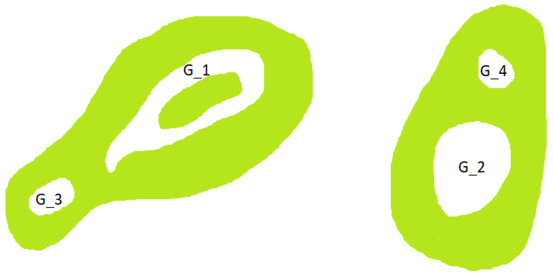
With Kenneth Falconer [5], we gave a different definition of thickness in ${\mathbb{R}}^d$ that is useful for sets of the cut-out type (see Figure 9 for an example).

Let $E\subset {\mathbb{R}}^d$ be an open path-connected set whose complement is a non-empty compact set, and let ${\left(G_n\right)}_n$ be a sequence of disjoint path-connected open sets contained in $E^C$. In the special case $d=1$, the set E is formed by the union of two disjoint open unbounded sets (this is the only case in which E is not a path-connected set). We say that E is the external component and ${\left(G_n\right)}_n$ is the sequence of gaps associated with the cut-out type of set

$$C:=E^C\backslash \bigcup _n{G}_n.$$

We can consider the sequence of gaps ordered by non-increasing diameter.

We define

$$\tau \left(C\right):=\underset{n\in \mathbb{N}}{inf}\frac{dist(G_n,{\bigcup }_{1\le i\le n-1}{G}_i\cup E)}{diam\left(G_n\right)}.$$

provided that there is at least one gap $G_n$. In case there are no gaps, we define

$$\tau \left(C\right):=\left\{\begin{array}{ccc}+\infty \hfill & \mathrm{if}& C^{\circ }\ne \varnothing \\ \\ 0\hfill & \mathrm{if}& C^{\circ }=\varnothing \end{array}\right.$$

(4)

This definition has certain advantages: it can take any value in $[0,\infty ]$, it is invariant under homothetic functions, and on the real line, it coincides with the classical one. In [5], we obtained a first extension to the Gap Lemma to ${\mathbb{R}}^d$ and also studied the intersections of countably many thick sets. However, there is a significant drawback: sets of positive thicknesses look like cut-out sets (“poking holes”). In particular, totally disconnected sets, which are of special interest in dynamical systems and fractal geometry, have a thickness of zero, and so this notion is not suitable for studying them.

5.2. Thickness in ${\mathbb{R}}^d$ (Useful in General, Even for Totally Disconnected Sets)

In [11], we were able to give a definition of thickness that is also useful for many totally disconnected sets and proved a higher-dimensional Gap Lemma, among other results.

From now on, we will work on ${\mathbb{R}}^d$ equipped with the distance ${dist}_{\infty }$ coming from the infinity norm, and all cubes (balls for this distance) will be closed. Recall that ${dist}_{\infty }(x,y):={\parallel x-y\parallel }_{\infty }:={max}_{1\le i\le d}|x_i-y_i|$. In fact, the notion of thickness and the results extend to any norm, but the infinity norm is the most useful one because cubes can be used to efficiently pack larger cubes (as opposed to, for example, Euclidean balls).

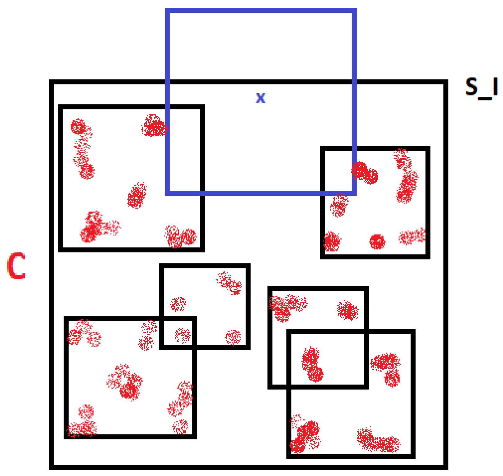
Given a word I (a finite sequence of natural numbers), we denote the length of I with $\ell \left(I\right)\in {\mathbb{N}}_0$. We say that $\left(S_I\right)$ is a system of cubes for a compact set C if

$$C=\bigcap _{n\in {\mathbb{N}}_0}\bigcup _{\ell \left(I\right)=n}{S}_I(\mathrm{Moran}\mathrm{construction}),$$

where the following are true:

• Each $S_I$ is a cube and contains ${\left\{S_{I,j}\right\}}_{1\le j\le k_I}$. No assumptions are made on the separation of the $S_{I,j}$.
• Every infinite word $i_1,i_2,\cdots$ of indices is of the construction

  $$\underset{n\to +\infty }{lim}rad\left(S_{i_1,i_2,\cdots ,i_n}\right)=0.$$

Note that any compact set arises from multiple systems of cubes, but for any $d\ge 2$, there is no canonical way to choose a system of cubes for a given set.

Let us fix a system of cubes $\left(S_I\right)$ for C. The main issue with extending the notion of thickness to compact sets in ${\mathbb{R}}^d$ is that there is not a suitable notion for a “gap”. We use the following notion as a substitute for the gap size (see Figure 10):

$$h_I:=\underset{x\in S_I}{max}{dist}_{\infty }(x,C).$$

Hence, $h_I$ is characterized by the properties that if $z\in S_I$ and $r\in [h_I,+\infty )$, then the closed cube $B(z,r)$ intersects C, but on the other hand, for every $r<h_I$, there is $z\in S_I$ such that $B(z,r)\cap C=\varnothing$.

Definition 6 (Thickness of C associated with the system of cubes ${\left\{S_I\right\}}_I$).

$$\tau (C,{\left\{S_I\right\}}_I):=\underset{n\in {\mathbb{N}}_0}{inf}\underset{\ell \left(I\right)=n}{inf}\frac{{min}_{i}rad\left(S_{I,i}\right)}{h_I}.$$

This definition preserves some of the basic properties of the Newhouse thickness. Indeed, on the real line, it agrees with Newhouse’s thickness (for the natural system of cubes arising in Newhouse’s definition). Thickness is invariant under homothetic functions (for the system of cubes obtained via mapping with the corresponding function). As in the real line, if a set has a large thickness, then it also has a large Hausdorff dimension, assuming that each cube has at least $M_0\ge 2$ non-overlapping children (a mild and reasonable assumption that is automatic on $\mathbb{R}$):

$${dim}_H\left(C\right)\ge \frac{d}{1+\frac{log(1+\frac{1}{\tau })}{log\left(M_0\right)}}.$$

See [11], Lemma 4 for more information.

Unlike Newhouse’s definition, the above notion of thickness depends on the system of cubes used to generate C. If the cubes provide a “bad approximation”, then the resulting value for $\tau$ can be artificial. To understand this, consider the example $C:=\left\{0\right\}\subseteq \mathbb{R}$ and the system of cubes that has just one cube in each level: ${\left\{[-\frac{1}{n},\frac{1}{n}]\right\}}_{n\in \mathbb{N}}$. Then $h_n=\frac{1}{n}$, and thus

$$\tau \left(C,\{{[-1/n,1/n\}}_{n\in \mathbb{N}}\right)=\underset{n\in \mathbb{N}}{inf}\frac{\frac{1}{n+1}}{\frac{1}{n}}=\underset{n\in \mathbb{N}}{inf}\frac{n}{n+1}=\frac{1}{2}.$$

However, intuitively, one expects the thickness of a singleton to be zero.

In order to state the Gap Lemma in ${\mathbb{R}}^d$, we need an additional condition which says that the children of any cube in the system are “well spread out”. Part of the motivation for this definition is to avoid pathological systems of cubes such as the above example:

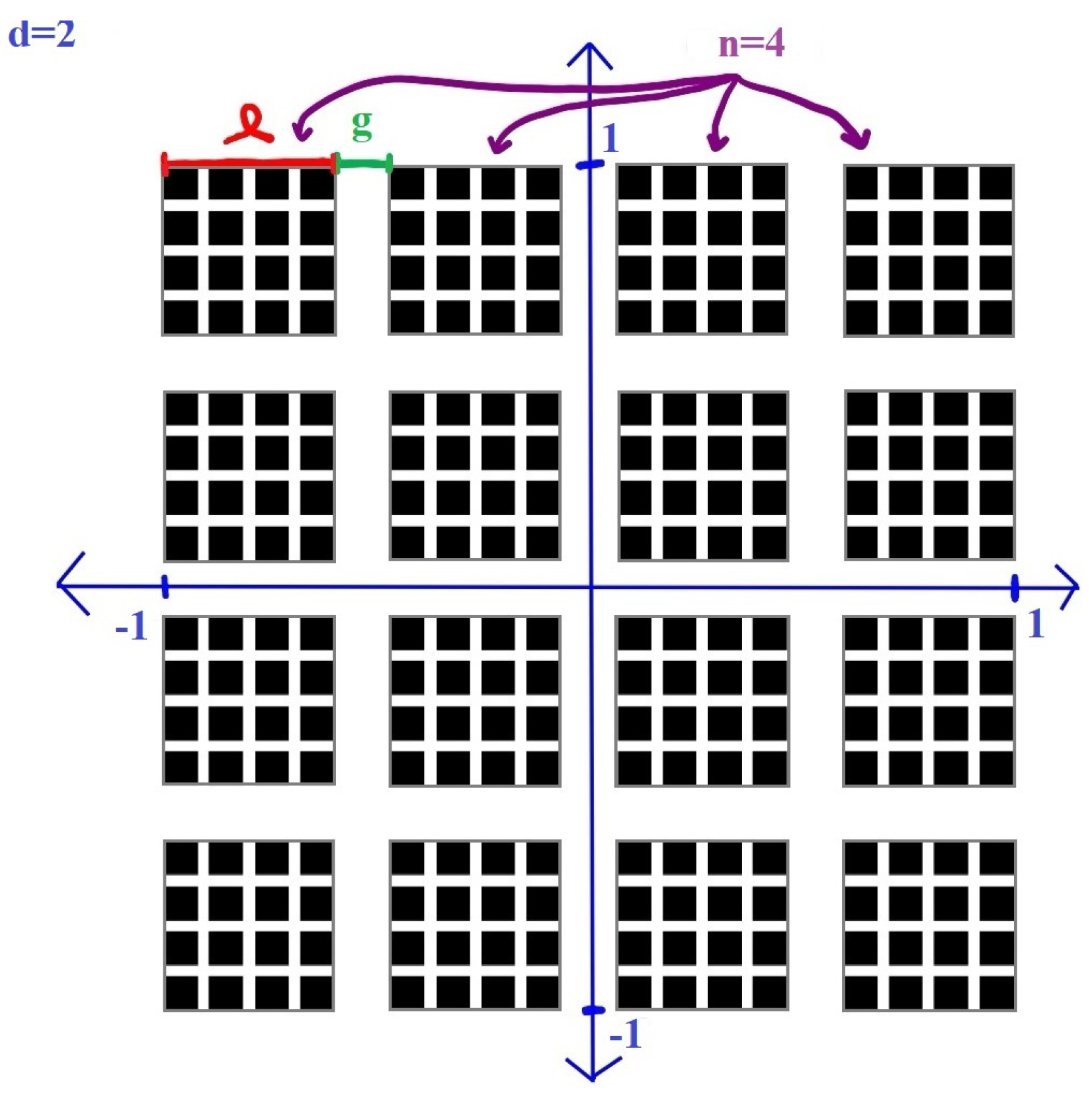
Definition 7.

We say that a system of cubes ${\left\{S_I\right\}}_I$ isr-uniformly dense if, for every I and for every cube $B\subseteq S_I$ with $rad\left(B\right)\ge rrad\left(S_I\right)$, there is a child $S_{I,i}\subseteq B$.

Let us consider an example. Fix $n\ge 2$ and $\ell \in (0,\frac{2}{n})$. We consider a corner Cantor set $C=C_{\ell ,n}\subseteq ({\mathbb{R}}^d,{dist}_{\infty })$, as in Figure 11. Let $g=\frac{2-n\ell }{n-1}$. One can check that the thickness is given by $\tau \left(C\right)=\frac{\ell }{g}=\frac{\ell (n-1)}{2-n\ell }$, and the set is $r:=\frac{1}{2}(2\ell +g)=\left(\ell +\frac{2-n\ell }{2(n-1)}\right)$-uniformly dense.

Theorem 5

(Higher dimensional Gap Lemma [11]). Let $C^1$ and $C^2$ be two compact sets in $({\mathbb{R}}^d,{dist}_{\infty })$, generated by systems of cubes ${\left\{S_I^1\right\}}_I$ and ${\left\{S_L^2\right\}}_L$, respectively, and fix $r\in (0,\frac{1}{2})$. Assume the following:

(1) 

$\tau (C^1,{\left\{S_I^1\right\}}_I)\tau (C^2,{\left\{S_L^2\right\}}_L)\ge \frac{1}{{(1-2r)}^2}$;

(2) 

${\left\{S_I^1\right\}}_I$ and ${\left\{S_L^2\right\}}_L$ are r-uniformly dense;

(3) 

$C^1\cap (1-2r)S_{\varnothing }^2\ne \varnothing$ and $rad\left(S_{\varnothing }^1\right)\ge rrad\left(S_{\varnothing }^2\right)$.

Then, we have

$$C^1\cap C^2\ne \varnothing .$$

Some remarks on this statement are in order. Unlike Newhouse’s Gap Lemma, we need the additional “uniform denseness” assumption. As mentioned above, this is partly for the above systems of cubes that yield artificially large values for the thickness.

Assumption (3) is quite mild, and it can be seen as a stronger version of the hypotheses (in the original Gap Lemma) that the convex hulls intersect and that each Cantor set is not contained in a gap of the other.

There is a balance between assumptions (1) and (2), as the first condition is stronger when r is close to $\frac{1}{2}$, and the second condition is stronger when r is close to 0. Note also that as $r\to 0$, assumption (1) reduces back to the product of the thicknesses being larger than one, as in the original Gap Lemma.

An important feature of Newhouses’s Gap Lemma is that the hypotheses are robust under perturbations of the Cantor sets. This is also the case for Theorem 5. For example, the assumptions are robust under $C^1$ perturbations whose derivatives are close to the identity applied to the sets, and if the sets are self-homothetic, they are also robust under perturbations of the generating iterated function system (see ([11], Lemmas 7 and 8 for details).

Recall that S. Biebler [27] defined a notion of thickness and proved the Gap Lemma for a class of dynamically defined compact sets in the plane. Even in this restricted context, Theorem 5 applies in many more cases (roughly speaking, Biebler has a more restrictive version of each of the assumptions). The definition of thickness and proof of the Gap Lemma are also significantly simpler than Biebler’s.

5.3. An Application to Directional Distance Sets

Given $E\subseteq {\mathbb{R}}^d$, the distance set of E is

$$\Delta \left(E\right):=\{\parallel x-y{\parallel }_2:x,y\in E\}\subseteq [0,\infty ).$$

It is a major open problem to understand the relationship between the sizes of E and $\Delta \left(E\right)$:

Conjecture 1 (Falconer’s distance conjecture).

If E is a compact set with${dim}_H\left(E\right)>d/2$, then$\Delta \left(E\right)$has a positive Lebesgue measure.

There are many partial results and variants. One of them involves investigating the conditions under which the distance set has a non-empty interior. The best result in this direction was due to Mattila and Sjölin:

Theorem 6

(Mattila and Sjölin [29]). If E is a compact set with ${dim}_H\left(E\right)>\frac{d+1}{2}$, then the distance set $\Delta \left(E\right)$ has a non-empty interior.

This result does not give quantitative bounds on the size of a ball in $\Delta \left(E\right)$, nor does it guarantee that zero is an interior point of $\Delta \left(E\right)$.

We know that sets with large thicknesses have large Hausdorff dimensions. Therefore, one can ask whether we can get stronger consequences for sets of large thicknesses. We will see that the Gap Lemma provides such a result.

For a fixed direction $v\in S^{(d-1)}$, we say that $t\ge 0$ is a distance between points of E in direction v if there are $e_1$ and $e_2$ in E such that $e_1-e_2=tv$. We define ${\Delta }_v\left(E\right)$ as the set of all distances between points in the set E in direction v. Of course, ${\Delta }_v\left(E\right)\subseteq \Delta \left(E\right)$.

By applying the Gap Lemma to E and $E-tv$, one can find that ${\Delta }_v\left(E\right)$ contains an explicit uniform interval for any direction v:

Corollary 1.

Let $E={\bigcap }_{n\ge 0}{\bigcup }_{\ell \left(I\right)=n}{S}_I$ be a compact set in ${\mathbb{R}}^d$ such that there exists $r\in (0,\frac{1}{3}]$, satisfying the following:

• $\tau (C,{\left\{S_I\right\}}_I)\ge \frac{1}{1-2r}$;
• ${\left\{S_I\right\}}_I$ is r-uniformly dense with respect to C.

Then, there is $a>0$ (depending only on r and the radius of $S_{⌀}$) such that for any direction $v\in S^{(d-1)}$, we have

$$[0,a]\subseteq {\Delta }_v\left(C\right).$$

Proof. 

We can assume without loss of generality that $S_{\varnothing }=B[0,1]$.

Let v be any vector in $S^{(d-1)}$. We are going to show that the sets C and $C+tv$ satisfy the hypothesis of the Gap Lemma (Theorem 5) for $t\in [\frac{-2r}{1-2r},\frac{2r}{1-2r}]$. Then, we will have $C\cap (C+tv)\ne \varnothing$ for any $t\in [0,\frac{2r}{1-2r}]$, and thus $[0,\frac{2r}{1-2r}]\subseteq {\Delta }_v\left(C\right)$.

By assumption, ${\left\{S_I\right\}}_I$ is uniformly dense with respect to C. Since the thickness is preserved by translations (also translating the system of balls), we have

$$\tau (C,{\left\{S_I\right\}}_I)\tau (C+tv,{\{S_I+tv\}}_I)\ge \frac{1}{{(1-2r)}^2}.$$

It remains to be shown that $C\cap (1-2r)\left(B[0,1]+tv\right)\ne \varnothing$. Since $r\in (0,\frac{1}{3}]$, we have that $(1-2r)\left(B[0,1]+tv\right)$ is a ball with a radius of at least r, and since $t\in [0,\frac{2r}{1-2r}]$, we have $(1-2r)\left(B[0,1]+tv\right)\subseteq B[0,1]$. Hence, by the r denseness, there is a child $S_i$ of $S_{\varnothing }$ contained in $(1-2r)\left(B[0,1]+tv\right)$. In particular, $C\cap (1-2r)\left(B[0,1]+tv\right)\ne \varnothing$. □

What is new compared with Mattila and Sjölin’s result is that this holds in every direction, and we obtain a uniform explicit interval containing zero. The assumptions, however, are much stronger.

5.4. Patterns in Thick Sets in ${\mathbb{R}}^d$

Recall from Theorem 4 that sets of large Newhouse thicknesses $\tau$ contain homothetic copies of all finite sets of certain explicit cardinality $N\left(\tau \right)$, and that this result is based on showing that thick sets are winning for the potential game. Both the result and the approach generalize to both our definitions of thickness in ${\mathbb{R}}^d$. In the case of Definition 6, the proof uses a variant of the game in which Alice erases neighborhoods of cube boundaries (spheres in the $d_{\infty }$ metric) instead of balls. Since the Gap Lemma is not used in the arguments, no denseness assumption is needed for these results. See [5], Theorem 7 and [11], Theorem 20 for details.

References

- Newhouse, S.E. Nondensity of axiom A(a) on S2. In Global Analysis; American Mathematical Society: Providence, RI, USA, 1970; pp. 191–202. [Google Scholar]
- Newhouse, S.E. The abundance of wild hyperbolic sets and nonsmooth stable sets for diffeomorphisms. Inst. Hautes Études Sci. Publ. Math. 1979, 50, 101–151. [Google Scholar] [CrossRef]
- Astels, S. Cantor sets and numbers with restricted partial quotients. Trans. Am. Math. Soc. 2000, 352, 133–170. [Google Scholar] [CrossRef]
- Boone, Z.; Palsson, E.A. A pinned Mattila–Sjölin type theorem for product sets. arXiv 2022, arXiv:2210.00675. [Google Scholar]
- Falconer, K.; Yavicoli, A. Intersections of thick compact sets in ℝd. Math. Z. 2022, 301, 2291–2315. [Google Scholar] [CrossRef]
- Hunt, B.R.; Kan, I.; Yorke, J.A. When Cantor sets intersect thickly. Trans. Am. Math. Soc. 1993, 339, 869–888. [Google Scholar] [CrossRef]
- McDonald, A.; Taylor, K. Finite point configurations in products of thick Cantor sets and a robust nonlinear Newhouse gap lemma. arXiv 2021, arXiv:2111.09393. [Google Scholar]
- Simon, K.; Taylor, K. Interior of sums of planar sets and curves. Math. Proc. Camb. Philos. Soc. 2020, 168, 119–148. [Google Scholar] [CrossRef] [Green Version]
- Williams, R.F. How big is the intersection of two thick Cantor sets. In Continuum Theory and Dynamical Systems (Arcata, CA, 1989)? American Mathematical Society: Providence, RI, USA, 1991; pp. 163–175. [Google Scholar]
- Yavicoli, A. Patterns in thick compact sets. Israel J. Math. 2021, 244, 95–126. [Google Scholar] [CrossRef]
- Yavicoli, A. Thickness and a gap lemma in ℝd. arXiv 2022, arXiv:2204.08428. [Google Scholar]
- Yu, H. Fractal projections with an application in number theory. Ergod. Theory Dyn. Syst. 2020. [Google Scholar] [CrossRef]
- Palis, J.; Takens, F. Hyperbolicity and sensitive chaotic dynamics at homoclinic bifurcations. In Cambridge Studies in Advanced Mathematics; Cambridge University Press: Cambridge, MA, USA, 1993; Volume 35. [Google Scholar]
- Falconer, K.J. The Geometry of Fractal Sets. Cambridge Tracts in Mathematics; Cambridge University Press: Cambridge, MA, USA, 1985. [Google Scholar]
- Falconer, K. Techniques in Fractal Geometry; John Wiley & Sons, Ltd.: Chichester, UK, 1997. [Google Scholar]
- Falconer, K. Fractal Geometry, 3rd ed.; John Wiley & Sons, Ltd.: Chichester, UK, 2014. [Google Scholar]
- Keleti, T. A 1-dimensional subset of the reals that intersects each of its translates in at most a single point. Real Anal. Exchange 1998/1999, 24, 843–844. [Google Scholar] [CrossRef]
- Keleti, T. Construction of one-dimensional subsets of the reals not containing similar copies of given patterns. Anal. PDE 2008, 1, 29–33. [Google Scholar] [CrossRef]
- Maga, P. Full dimensional sets without given patterns. Real Anal. Exchange 2010/2011, 36, 79–90. [Google Scholar] [CrossRef]
- Máthé, A. Sets of large dimension not containing polynomial configurations. Adv. Math. 2017, 316, 691–709. [Google Scholar] [CrossRef] [Green Version]
- Yavicoli, A. Large sets avoiding linear patterns. Proc. Am. Math. Soc. 2021, 149, 4057–4066. [Google Scholar] [CrossRef] [Green Version]
- Sahlsten, T.; Kuca, B.; Orponen, T. On a continuous Sárközy type problem. arXiv 2022, arXiv:2110.15065. [Google Scholar]
- Chan, V.; Łaba, I.; Pramanik, M. Finite configurations in sparse sets. J. Anal. Math. 2016, 128, 289–335. [Google Scholar] [CrossRef] [Green Version]
- Henriot, K.; Łaba, I.; Pramanik, M. On polynomial configurations in fractal sets. Anal. PDE 2016, 9, 1153–1184. [Google Scholar] [CrossRef] [Green Version]
- Łaba, I.; Pramanik, M. Arithmetic progressions in sets of fractional dimension. Geom. Funct. Anal. 2009, 19, 429–456. [Google Scholar]
- Broderick, R.; Fishman, L.; Simmons, D. Quantitative results using variants of Schmidt’s game: Dimension bounds, arithmetic progressions, and more. Acta Arith. 2019, 188, 289–316. [Google Scholar] [CrossRef] [Green Version]
- Biebler, S. A complex gap lemma. Proc. Am. Math. Soc. 2020, 148, 351–364. [Google Scholar] [CrossRef]
- Feng, D.-J.; Wu, Y.-F. On arithmetic sums of fractal sets in ℝd. J. Lond. Math. Soc. 2021, 104, 35–65. [Google Scholar] [CrossRef]
- Mattila, P.; Sjölin, P. Regularity of distance measures and sets. Math. Nachr. 1999, 204, 157–162. [Google Scholar] [CrossRef]
Figure 1.
Construction of a compact set.
Figure 2.
Removing gaps of equal length in two possible orders.
Figure 3.
The middle Cantor set.
Figure 4.
Linked intervals.
Figure 5.
Hausdorff dimension.
Figure 6.
The region R.
Figure 7.
One step in Keleti’s construction of a compact set that avoids progressions.
Figure 8.
The region of possible pairs .
Figure 9.
Step 4 of construction of a cut-out type of set.
Figure 10.
The radius of the blue square is the substitute of the notion of the gap size.
Figure 11.
A corner Cantor set.
Publisher’s Note: MDPI stays neutral with regard to jurisdictional claims in published maps and institutional affiliations. |
© 2022 by the author. Licensee MDPI, Basel, Switzerland. This article is an open access article distributed under the terms and conditions of the Creative Commons Attribution (CC BY) license (https://creativecommons.org/licenses/by/4.0/).
Share and Cite
MDPI and ACS Style
Yavicoli, A. A Survey on Newhouse Thickness, Fractal Intersections and Patterns. Math. Comput. Appl. 2022, 27, 111. https://doi.org/10.3390/mca27060111
AMA Style
Yavicoli A. A Survey on Newhouse Thickness, Fractal Intersections and Patterns. Mathematical and Computational Applications. 2022; 27(6):111. https://doi.org/10.3390/mca27060111
Chicago/Turabian StyleYavicoli, Alexia. 2022. "A Survey on Newhouse Thickness, Fractal Intersections and Patterns" Mathematical and Computational Applications 27, no. 6: 111. https://doi.org/10.3390/mca27060111