
Spherical Distributions Used in Evolutionary Algorithms

1
Department of Applied Mathematics, Faculty of Economic Cybernetics, Statistics and Informatics, Bucharest University of Economic Studies, Calea Dorobantilor 15-17, 010552 Bucharest, Romania
2
“Gheorghe Mihoc—Caius Iacob” Institute of Mathematical Statistics and Applied Mathematics of the Romanian Academy, 050711 Bucharest, Romania
Mathematics 2021, 9(23), 3098; https://doi.org/10.3390/math9233098
Submission received: 22 October 2021
/
Revised: 16 November 2021
/
Accepted: 27 November 2021
/
Published: 30 November 2021
(This article belongs to the Special Issue Probability, Stochastic Processes and Optimization)
Abstract
:Performance of evolutionary algorithms in real space is evaluated by local measures such as success probability and expected progress. In high-dimensional landscapes, most algorithms rely on the normal multi-variate, easy to assemble from independent, identically distributed components. This paper analyzes a different distribution, also spherical, yet with dependent components and compact support: uniform in the sphere. Under a simple setting of the parameters, two algorithms are compared on a quadratic fitness function. The success probability and the expected progress of the algorithm with uniform distribution are proved to dominate their normal mutation counterparts by order .
1. Introduction
Probabilistic algorithms are among the most popular optimization techniques due to their easy implementation and high efficiency. Their roots can be traced back to the first random walk problem proposed by Pearson in 1905: “A man starts from a point O, and walks ℓ yards in a straight line; he then turns through any angle whatever, and walks another ℓ yards in a second straight line. He repeats this process n times. I require the probability that after these n stretches he is at a distance between r and from his starting point O.” [1,2,3,4].
Using the ability of computers to generate and store large samples from multi-variate distributions, physicists and engineers have transformed the original random walk into a powerful optimization tool. Probabilistic algorithms do not require additional information on the fitness function, they simply generate potential candidate solutions, select the best, and move on.
Sharing the same random generator, yet differing with respect to the selection phase, two classes of probabilistic algorithms became more popular over the last decades: simulated annealing (also known as Metropolis or Hastings algorithm) [5] and evolutionary algorithms (EAs) [6,7]. Only the latter will be discussed in this paper.
EAs are assessed based on local quantities, such as success probability and progress rate, respectively, on global measures, like expected convergence time. Performance depends on both the fitness landscape, and on the particular probabilistic scheme (leading to a probability distribution) involved in the generating-selection mechanism. A popular test problem consists in minimizing the quadratic SPHERE function (To avoid confusion, we use uppercase for the fitness function, and lowercase for the uniform distribution in/on the sphere.), with optimum in the origin.
An elitist (that is, keeping always the best solution found so far), one-individual, mutation+selection EA is depicted below (Algorithm 1).
| Algorithm 1 An elitist, one-individual, mutation+selection EA. |
Set and the initial point of the algorithm, Repeat Mutation: generate a new point according to a multi-variate distribution Selection:if then else Until , for some fixed |
The region of success of Algorithm 1 is
A rigorous description of the long-term behavior of EAs involves renewal processes, drift analysis, order statistics, martingales, or other stochastic processes [7,8,9,10,11,12,13]. However, the basic structure is that of a Markov chain, as the algorithm’s state at the next iteration depends only on its current state. Difficulties occur when, even for simple fitness functions, SPHERE included, the actual position of the algorithm affects significantly the local behavior, such that the process lacks homogeneity; so begins the search for powerful mathematical tools, able to describe the transition kernel, which encapsulates the local probabilistic structure of the algorithm [6,7].
For any fitness function and fixed point , assumed as current state, the transition kernel provides the probability of the algorithm to be in set at the next step. Even if the mutation distribution has a probability density function (pdf), discontinuity occurs due to the disruptive effect of elitist selection. To make that clear, let us denote the mutation random variable by , its pdf by f, and cumulative distribution function (cdf) by F. The singular (Dirac) distribution, that loads only one point, is denoted . Index x designates conditioning by the current state. The finite time behavior of the algorithm is inscribed in the random variable and the next state of the algorithm, provided the current state, is x.
while the (Markov) transition kernel carries the local transition probabilities
As the mutation distribution is entirely responsible for the evolution of the algorithm, let us take a look at the possible candidates, the multi-variate distributions.
Let denote some n-dimensional random variable, and the euclidean norm in be . The n-dimensional sphere of radius 1, its surface and volume are given by [14]
We use ‘bold-face’ for (single, or multi-variate) random variables, and ‘normal-face’ for real numbers (or vectors). When partitioning the n dimensions into two sets and with , we use the compact notation , for either vectors or random variables. Unless otherwise stated, denotes the beta random variable with support and parameters , while and stand for the corresponding coefficients. The (one-dimensional) uniform random variable with support is denoted . The sign denotes two random variables with identical cdf.
The class of spherical distributions can be defined in a number of equivalent ways, two of which are depicted below ([15], pp. 30, 35) (See the excellent monograph of Fang et al. [15] for an exhaustive introduction to spherical distributions.):
Definition 1.
- An n-dimensional random variable is said to have spherically symmetric distribution(or simply spherical distribution) iffor some one-dimensional random variable (radius) , and the uniform distribution on the unit sphere . Moreover, and are independent, and also
- If the spherical distribution has pdf g, then g satisfies , and there is a special connection between g and f, the pdf of , namely,
Three spherical distributions are of particular interest in our analysis:
- the uniform distribution on the unit sphere, with support , denoted ;
- the uniform distribution in (inside) the unit sphere, with support , denoted simply UNIFORM in this paper; and
- the standard normal distribution, denoted or simply NORMAL.
A comparison of the previous distributions can be performed from many angles. NORMAL was the first discovered, applied, and thoroughly analyzed in statistics, as being one of the only spherical distributions with independent and identically distributed marginals. By contrast, the components of uniform distributions on/in the sphere are not independent, neither uniform (However, the conditional marginals are uniform, see Theorem 5). Recently, the scientific interest shifted to uniform multi-variate distributions, following the increasing application of directional statistics to earth sciences and quantum mechanics [16,17], and also the application of Dirichlet distribution (which lies at the basis of spherical analysis) to Bayesian inference, involved in medicine, genetics, and text-mining [18].
From the computer science point of view, uniform and normal distributions share an entangled history, in at least two areas: random number generators and probabilistic optimization algorithms. With respect to the first area, early approaches to sampling from the uniform distribution on sphere were actually using multi-normal random generators to produce a sample x, which was further divided by , following Equation (7). Nowadays, the situation changed, with the appearance of a new class of algorithms which circumvent the usage of the normal generator by using properties of marginal uniform distributions on/in spheres [17,19]. The comparison of mean computation times demonstrates that the uniform sampling method outperforms the normal generator for dimensions up to [20].
Concerning global optimization, the probabilistic algorithms based on the two distribution types evolved at the same time, although with few overlaps. In the theory and practice of real space (continuous) EA-evolution strategy being their most popular, the representative-normal distribution has played, from the beginning, the central role. Therefore, there is a great amount of literature stressing out the advantages of this distribution [6,21,22].
Occasionally, the supremacy of the normal operator has been challenged by theoretical studies that proposed different mutation distributions, such as uniform in the cube (which is non-spherical) [10], uniform on the sphere [7,23], uniform in the sphere [9], or even the Cauchy distribution [24]. An attempt to solve the problem globally, by considering the whole class of spherical (isotropic) distributions, was made in [25,26]. These approaches yielded only limited results (valid either for small space dimension n, or for ), or not so tight lower/upper bounds for the expected progress of the algorithm.
The study of EAs with uniform distribution in the sphere recently culminated with two systematic studies, one for RIDGE [27], the other for SPHERE [28], comparable to classical theory of evolution strategies [6,29]. Under a carefully constructed normalization of mutation parameters (equalizing the expectations of normal and uniform multi-variates as ), those studies demonstrate the same behavior for the respective EA variants. Intuitively, the explanation is that for large dimensions, both normal and uniform distributions concentrate on the surface of the sphere. The present paper differs from the previous analyses in the way that it does not apply any normalization of parameters. As a consequence, the results are different from those in [28] and an actual comparison between the two algorithms can be achieved.
Section 2 discusses the general framework of spherical multi-variate distributions, with special focus on uniform and normal. Then, two algorithms, one with uniform mutation and the other with normal mutation, are compared on the SPHERE fitness function with respect to their local performance in Section 3.
2. Materials and Methods. Spherical Distributions
In light of Definition 1, the spherical distributions are very much alike. They all exhibit stochastic representation (6), that is, each can be generated as a product of two independent distributions, the n-dimensional uniform on the sphere and some scalar, positive random variable . As the distribution of makes the whole difference, we point out the form of this random variable in the three cases of interest.
- - is obviously the Dirac distribution in 1:
- UNIFORM- is distributed , with pdf ([15], p. 75):
Using as primary source the monograph [15], we next discuss in more detail the stochastic properties of the UNIFORM and NORMAL multi-variates, the two candidates for the mutation operator of the algorithm.
2.1. Uniform in the Sphere
The local analysis of the EA is based on two particular marginal distributions: the first component , and the joint marginal of the remaining components, . As already pointed out, the marginals of UNIFORM are not independent random variables, and we shall see that neither are they uniform. A general formula for the marginal density is provided in [15] (p. 75):
Theorem 1.
If is uniformly distributed in the unit sphere, with of dimension k, , then the marginal density of is
Corollary 1.
The pdf of the first component of UNIFORM is
Using the symmetry with respect to the origin and substituting in function (13), we obtain an interesting result, previously unreported in spherical distributions literature.
Corollary 2.
The square of the first component of UNIFORM is , with pdf
The density of the last components can be derived also from Theorem 1.
Corollary 3.
The joint pdf of the last components of UNIFORM is
As function of several variables, formula (15) might not look very appealing; however, a basic result from spherical distribution theory transforms the corresponding multiple integral into a scalar one ([15], p. 23).
Theorem 2.
(Dimension reduction).
One can see now that, if is uniformly distributed in the unit sphere, the sum of squares of the last components is distributed.
Corollary 4.
Let be UNIFORM. Then, the one-dimensional random variable is , with pdf
As the components of the uniform distribution on/in the sphere are not independent, a better understanding of the nature of such distributions is provided by conditioning one component with respect to the others. In case of uniform distribution on the sphere, the work in [15] (p. 74) states that all the conditional marginals are also uniform on the sphere.
We shall see that a similar characterization holds true for the uniform in the sphere. This result is not presented in [15] and, to the best of our knowledge, in no other reference on spherical distributions. Therefore, an additional theorem is needed ([30], p. 375).
Theorem 3.
Let be a spherical distribution and , where is m-dimensional, . Then the conditional distribution of given with is given by
For each , and are independent, and the cdf of is given by
for and , F being the cdf of .
We prove now the result on conditional marginals of the uniform distribution in the unit sphere. As conditioning the first component with respect to all others is the most relevant for EA analysis, this particular case is stressed out.
First, an old result from probability theory is needed, similar to the convolution operation, but for the product of two independent random variables [31].
Theorem 4.
(Mellin’s formula). Let and be two independent, non-negative random variables, with densities g and h. Then, has pdf
Note that Mellin’s formula still holds, if only one of the random variables is continuous, the other being discrete, see, e.g., in [15] (p. 41).
Theorem 5.
- Let be UNIFORM, where is m-dimensional, . The conditional distribution of given is UNIFORM in the m dimensional sphere with radius .
- If and is a point in with , the conditional distribution of given is
Proof.
We begin with the last part, case .
Equation (18) gives the conditional first component as a product of two independent random variables, the second being the one-dimensional UNIFORM-the discrete random variable that loads and 1 with equal probability, .
The cdf of the first random variable is given by (19), as a fraction of two integrals, both with respect to F, the cdf of . In case of UNIFORM, is given by (11), thus .
If , the upper and lower integrals in (19) are equal, so the probability is 1. If , the upper integral is
while the lower one is
Thus, for any fixed , the cdf of the conditional radius is
while the corresponding pdf is
Back to the application of Theorem 3, Equation (18). The conditional first component of UNIFORM is a product of two independent random variables: one continuous, the other discrete. This is the easy version of Mellin’s formula, and the result is the continuous uniform random variable with support from Equation (21).
As for a larger dimension, , the cdf in (19) becomes
with corresponding pdf
which is , yet with reduced support.
2.2. Normal
As we did with UNIFORM, we denote the first component of the standard normal multi-variate distribution by , and the remaining components by . Due to independence of the marginals, one can write a compact equivalent of Propositions 1 and 3, see, e.g., in [6] (p. 54).
Proposition 1.
Let be NORMAL.
- The pdf of the first component, , is
- The joint pdf of the last components, , is
Due to sphericity of the joint components, one obtains again a compact form for the sum of squares.
Corollary 5.
The one-dimensional random variable is with degrees of freedom, with pdf
3. Results
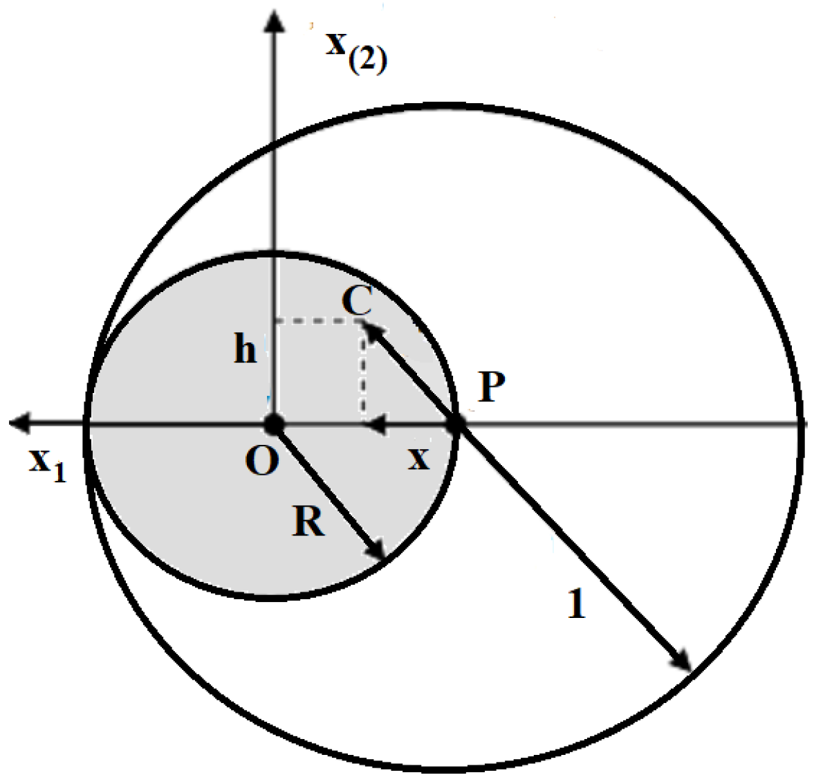
We restrict the study to the case P (current algorithm position) nearby O (optimum of SPHERE) and analyze the local performance of two EAs, one with uniform, the other with normal mutation, in terms of success probability and expected progress. Namely, we assume , such that success region is the sphere with center O and radius R, Figure 1.
Re-set P as the origin of the coordinate system, and measure the algorithm’s progress in the positive direction of the first axis-write x for , h for and u for . The success probability and the expected progress are provided by the first term of transition kernel (4), respectively, by the upper part of random variable (3). They obey to the uniform continuous mutation distribution with pdf and compact support, the sphere with center P and radius 1.
The calculus of success probability and expected progress resides in integrating the random variable (3) over . For UNIFORM mutation this calculus is analytically tractable. For NORMAL mutation, the analytic integration is impossible, see in [6] (p. 56) and Theorem 8, but the theory of incomplete Gamma functions makes the comparison tractable.
Note that, if the success probability bears only one possible definition (the volume of success region), the situation is different with respect to the expected progress. As the random variable from (3) characterizes the local behavior of the algorithm, one would normally associate the expected progress to the expected value of this random variable. However, is n-dimensional, and such is , so there is a need to mediate somehow among the n components.
One could consider only the first component of the expected value, the one pointing towards the optimum, which has been applied on a different fitness landscape, the inclined plane [21]. (Yet in another landscape, the RIDGE, it is customary to consider the progress along the perpendicular component h, see in [6,27] for an inventory of fitness functions used in EA testing, the reader is referred to the work in [32].) For UNIFORM mutation, a simplified version of the expected progress may be defined as the centroid of the corresponding success region [9,10]. However, a more traditional view is followed here ([6], p. 54):
This corresponds to the difference in distance , provided is a random point generated by mutation, Figure 1.
3.1. Uniform Mutation
If the UNIFORM mutation in the unit sphere with center P is applied, one cannot use for integration the ensemble of Propositions 1 and 3, as the marginals of UNIFORM are not independent. Instead, one should use the conditional first component from Theorem 5, together with the joint dimensional distribution from Proposition 3. The integration region is
Theorem 6.
Let an EA with UNIFORM mutation minimizing the SPHERE be situated at current distance R from the origin, . The success probability is
Theorem 7.
Let an EA with UNIFORM mutation minimizing the SPHERE be situated at current distance R from the origin, . The expected progress is
Proof.
Following the proof of Theorem 6 and inserting factor (25), one gets
Again, is the integral (27), multiplied by , thus
The substitution on provides
while partial integration gives
Bringing in the constant C, one gets
The results from Theorems 6 and 7 are also presented in [28], yet with different proofs. Equations (26) and (28) point out a remarkable property of the EA with UNIFORM mutation on the SPHERE.
Corollary 6.
In the conditions of Theorems 6 and 7, the success probability is the derivative of the expected progress.
3.2. Normal Mutation
Setting and avoiding the transformation , one obtains the success probability and the expected progress for the EA with standard normal mutation following closely the proof in ([6], pp. 54–56). The incomplete Gamma function is ([33], p. 260):
The following expressions are not restricted to the case of algorithm nearby optimum, due to the unbounded support of the normal distribution. Unfortunately, integration is impossible.
Theorem 8.
Let an EA with NORMAL mutation minimizing the SPHERE be situated at current distance R from the origin.
- The success probability is
- The expected progress is
Proof.
The same calculus applies for the expected progress, with the addition of the factor corresponding to the one dimensional progress along the x axis, Equation (25). □
3.3. Comparison
Due to the analytic intractability of integral representations (34) and (35), a theoretical comparison between two variants of Algorithm 1-one with UNIFORM, the other with NORMAL mutation-must resort to inequalities. Therefore, a deeper insight into the prolific theory of Euler and hypergeometric functions is required. We start with an upper bound for the incomplete Gamma function (33) ([34], p. 1213).
Proposition 2.
The following inequality holds
Proposition 3.
(Hypergeometric functions).
- For any real set of parameters and any real number x, definewhere is the Pochhammer symbol, with
- If and , we write , if
- If , the following inequality holds:
We can prove now the main result stating that, for an EA acting on the SPHERE with current position at maximal range from the origin, the UNIFORM mutation provides a larger success probability than the NORMAL mutation, for the arbitrary dimension n. We denote by the double factorial (semi-factorial), that is, the product of all integers from 1 to n of same parity with n.
Theorem 9.
Let an EA minimizing the SPHERE be situated at current distance R from the origin, such that . For any , the following holds:
Proof.
Using the series expansion of the exponential, the second integral in (43) becomes a hypergeometric function of type (38). The interchange of the integral and the sum is justified by the absolute convergence of the series.
In the last equality we have used Equation (26) and the definition of the double factorial, for n even. Obviously, for n odd the constant will appear at the tail of the product, yet this is a minor difference that may be neglected. □
The result for the expected progress follows now easily.
Theorem 10.
Let an EA minimizing the SPHERE be situated at current distance R from the origin, such that . For any , the following holds:
4. Discussion
Within evolutionary algorithms acting on real space, the use of normal distribution makes the implementation easier: in order to generate an n dimensional point, one simply generates n times from the normal uni-variate. Unfortunately, simplicity of the practical algorithm does not transfer to the theoretical analysis, making EA experts go long distances in order to estimate performance quantities like the success probability and the expected progress. In the end, the normal mutation only provides asymptotic formulas, valid for large n.
This paper analyzes a different mutation operator, based on the uniform multi-variate in the sphere, with dependent components. Using deeper insights into the spherical distributions theory, the local performance of the algorithm with uniform mutation was measured on the SPHERE fitness function. Close expressions for the success probability and the expected progress of the EA with uniform mutation have been derived, valid for arbitrary n. Compared to the performance of the normal operator-which, due to the intractability of integral formulas in Theorem 8, required inequalities with hypergeometric functions-, the success probability and the expected progress of the algorithm with uniform mutation are both larger, by a factor of order .
5. Conclusions
From a broader perspective, this paper can be seen, together with the works in [27,28], as an attempt of revisiting the classical theory of continuous evolutionary algorithms. Even if practitioners in the field will continue to use the normal multi-variate as mutation distribution, we claim that the theory can benefit from the uniform distribution inside the sphere. First, as demonstrated in this paper, a particular setting of parameters (the natural choice ) provides better performance for the uniform mutation operator on the SPHERE landscape, if current position of the algorithm is nearby the optimum. However, in light of the “no free-lunch theorem for optimization” paradigm [39], one cannot expect general dominance of an algorithm over all others, irrespective of the fitness function. Rather, specific algorithms with particular operators should be analyzed separately, on different optimization landscapes. This is where the second advantage of the new uniform distribution occurs, in terms of more tractable mathematical analysis, yielding close formulas, previously not attained by normal mutation theory—see the studies of the RIDGE landscape in [28] and of the elitist evolutionary algorithm with mutation and crossover on SPHERE in [27].
A theory of continuous evolutionary algorithms could not be complete without the analysis of global behavior and adaptive mutation parameter. These cases have already been treated in [27,28]—under a normalization of mutation sphere radius which makes algorithm behave similarly to the one with normal mutation, in terms of difference and differential equations, following the works in [6,29]. This opens the way for the challenging task, previously unattempted in probabilistic optimization literature, of linking the theory of continuous evolutionary algorithms to that of differential optimization techniques such as particle swarm optimization [40] and differential evolution [41].
Funding
The work was supported by the Bucharest University of Economic Studies, Romania, through Project “Mathematical modeling of factors leading to subscription or un-subscription from email and SMS lists, forums and social media groups”.
Acknowledgments
The author is grateful to his colleague Ovidiu Solomon for guidance through the jungle of Hypergeometric functions.
Conflicts of Interest
The authors declare no conflict of interest.
References
- Pearson, K. The problem of the random walk. Nature 1905, 72, 294. [Google Scholar] [CrossRef]
- Kluyver, J.C. A local probability problem. Nederl. Acad. Wetensch. Proc. 1905, 8, 341–350. [Google Scholar]
- Watson, G.N. A Treatise on the Theory of Bessel Functions; University Press: Cambridge, UK, 1995. [Google Scholar]
- Zhou, Y. On Borwein’s conjectures for planar uniform random walks. J. Aust. Math. Soc. 2019, 107, 392–411. [Google Scholar] [CrossRef] [Green Version]
- Dunson, D.B.; Johndrow, J.E. The Hastings algorithm at fifty. Biometrika 2020, 107, 1–23. [Google Scholar] [CrossRef] [Green Version]
- Beyer, H.-G. The Theory of Evolution Strategies; Springer: Heidelberg, Germany, 2001. [Google Scholar]
- Rudolph, G. Convergence Properties of Evolutionary Algorithms; Kovać: Hamburg, Germany, 1997. [Google Scholar]
- Agapie, A.; Wright, A.H. Theoretical analysis of steady state genetic algorithms. Appl. Math. 2014, 59, 509–525. [Google Scholar] [CrossRef] [Green Version]
- Agapie, A.; Agapie, M.; Rudolph, G.; Zbaganu, G. Convergence of evolutionary algorithms on the n-dimensional continuous space. IEEE Trans. Cybern. 2013, 43, 1462–1472. [Google Scholar] [CrossRef] [PubMed]
- Agapie, A.; Agapie, M.; Zbaganu, G. Evolutionary Algorithms for Continuous Space Optimization. Int. J. Syst. Sci. 2013, 44, 502–512. [Google Scholar] [CrossRef]
- Agapie, A. Estimation of Distribution Algorithms on Non-Separable Problems. Int. J. Comp. Math. 2010, 87, 491–508. [Google Scholar] [CrossRef]
- Agapie, A. Theoretical analysis of mutation-adaptive evolutionary algorithms. Evol. Comp. 2001, 9, 127–146. [Google Scholar] [CrossRef]
- Auger, A. Convergence results for the (1,λ)-SA-ES using the theory of ϕ-irreducible Markov chains. Theor. Comput. Sci. 2005, 334, 35–69. [Google Scholar] [CrossRef] [Green Version]
- Li, S. Concise Formulas for the Area and Volume of a Hyperspherical Cap. Asian J. Math. Stat. 2011, 4, 66–70. [Google Scholar] [CrossRef] [Green Version]
- Fang, K.-T.; Kotz, S.; Ng, K.-W. Symmetric Multivariate and Related Distributions; Chapman and Hall: London, UK, 1990. [Google Scholar]
- Mardia, K.V.; Jupp, P.E. Directional Statistics; Wiley: New York, NY, USA, 2000. [Google Scholar]
- Watson, G.S. Statistics on Spheres; University of Arkansas Lecture Notes in the Mathematical Sciences; Wiley: New York, NY, USA, 1983. [Google Scholar]
- Blei, D.M.; Ng, A.Y.; Jordan, M.I. Latent Dirichlet allocation. J. Mach. Learn. Res. 2003, 3, 993–1022. [Google Scholar]
- Fang, K.-T.; Yang, Z.; Kotz, S.; Ng, K.-W. Generation of multivariate distributions by vertical density representation. Statistics 2001, 35, 281–293. [Google Scholar] [CrossRef]
- Harman, R.; Lacko, V. On decompositional algorithms for uniform sampling from n-spheres and n-balls. J. Multivar. Anal. 2010, 101, 2297–2304. [Google Scholar] [CrossRef] [Green Version]
- Rechenberg, I. Evolutionsstrategie: Optimierung Technischer Systeme Nach Prinzipiender Biologischen Evolution; Frommann-Holzboog Verlag: Stuttgart, Germany, 1973. [Google Scholar]
- Schwefel, H.-P. Evolution and Optimum Seeking; Wiley: New York, NY, USA, 1995. [Google Scholar]
- Schumer, M.A.; Steiglitz, K. Adaptive Step Size Random Search. IEEE Trans. Aut. Control 1968, 13, 270–276. [Google Scholar] [CrossRef] [Green Version]
- Rudolph, G. Local convergence rates of simple evolutionary algorithms with Cauchy mutations. IEEE Trans. Evol. Comp. 1997, 1, 249–258. [Google Scholar] [CrossRef]
- Jägersküpper, J. Analysis of a simple evolutionary algorithm for minimisation in Euclidean spaces. In International Colloquium on Automata, Languages, and Programming; Lecture Notes in Computer Science; Springer: New York, NY, USA, 2003; Volume 2719, pp. 1068–1079. [Google Scholar]
- Jägersküpper, J.; Witt, C. Rigorous runtime analysis of a (μ+1) ES for the sphere function. In Proceedings of the 7th Annual Conference on Genetic and Evolutionary Computation, Washington, DC, USA, 25–29 June 2005; pp. 849–856. [Google Scholar]
- Agapie, A.; Solomon, O.; Giuclea, M. Theory of (1+1) ES on the RIDGE. IEEE Trans. Evol. Comp. 2021, 2021. [Google Scholar] [CrossRef]
- Agapie, A.; Solomon, O.; Bădin, L. Theory of (1+1) ES on SPHERE revisited. 2021. under review. [Google Scholar]
- Beyer, H.-G. On the performance of (1, λ)-evolution strategies for the ridge function class. IEEE Trans. Evol. Comput. 2001, 5, 218–235. [Google Scholar] [CrossRef]
- Cambanis, S.; Huang, S.; Simons, G. On the Theory of Elliptically Contoured Distributions. J. Mult. Anal. 1981, 11, 368–385. [Google Scholar] [CrossRef] [Green Version]
- Huntington, E.V. Frequency Distribution of Product and Quotient. Ann. Math. Statist. 1939, 10, 195–198. [Google Scholar] [CrossRef]
- Huang, H.; Su, J.; Zhang, Y.; Hao, Z. An Experimental Method to Estimate Running Time of Evolutionary Algorithms for Continuous Optimization. IEEE Trans. Evol. Comput. 2020, 24, 275–289. [Google Scholar] [CrossRef]
- Abramowitz, M.; Stegun, I.A. (Eds.) Handbook of Mathematical Functions, 9th ed.; Dover: New York, NY, USA, 1972. [Google Scholar]
- Neuman, E. Inequalities and Bounds for the Incomplete Gamma Function. Results Math. 2013, 63, 1209–1214. [Google Scholar] [CrossRef]
- Volkmer, H.; Wood, J.J. A note on the asymptotic expansion of generalized hypergeometric functions. Anal. Appl. 2014, 12, 107–115. [Google Scholar] [CrossRef]
- Slater, L.J. Generalized Hypergeometric Functions; University Press: Cambridge, UK, 1966. [Google Scholar]
- Karp, D.B. Representations and Inequalities for Generalized Hypergeometric Functions. J. Math. Sci. 2015, 207, 885–897. [Google Scholar] [CrossRef] [Green Version]
- Luke, Y.L. Inequalities for generalized hypergeometric functions. J. Approx. Theory 1972, 5, 41–65. [Google Scholar] [CrossRef] [Green Version]
- Wolpert, D.H.; Macready, W.G. No free lunch theorems for optimization. IEEE Trans. Evol. Comp. 1997, 1, 67–82. [Google Scholar] [CrossRef] [Green Version]
- Kadirkamanathan, V.; Selvarajah, K.; Fleming, P.J. Stability analysis of the particle dynamics in particle swarm optimizer. IEEE Trans. Evol. Comp. 2006, 10, 245–255. [Google Scholar] [CrossRef]
- Dasgupta, S.; Das, S.; Biswas, A.; Abraham, A. On stability and convergence of the population-dynamics in differential evolution. AI Commun. 2009, 22, 1–20. [Google Scholar] [CrossRef] [Green Version]
Figure 1.
Success region of Algorithm 1 with uniform mutation on SPHERE.

Publisher’s Note: MDPI stays neutral with regard to jurisdictional claims in published maps and institutional affiliations. |
© 2021 by the author. Licensee MDPI, Basel, Switzerland. This article is an open access article distributed under the terms and conditions of the Creative Commons Attribution (CC BY) license (https://creativecommons.org/licenses/by/4.0/).
Share and Cite
MDPI and ACS Style
Agapie, A. Spherical Distributions Used in Evolutionary Algorithms. Mathematics 2021, 9, 3098. https://doi.org/10.3390/math9233098
AMA Style
Agapie A. Spherical Distributions Used in Evolutionary Algorithms. Mathematics. 2021; 9(23):3098. https://doi.org/10.3390/math9233098
Chicago/Turabian StyleAgapie, Alexandru. 2021. "Spherical Distributions Used in Evolutionary Algorithms" Mathematics 9, no. 23: 3098. https://doi.org/10.3390/math9233098
Note that from the first issue of 2016, this journal uses article numbers instead of page numbers. See further details here.