Blood Coagulation Algorithm: A Novel Bio-Inspired Meta-Heuristic Algorithm for Global Optimization

Abstract

This paper introduces a novel population-based bio-inspired meta-heuristic optimization algorithm, called Blood Coagulation Algorithm (BCA). BCA derives inspiration from the process of blood coagulation in the human body. The underlying concepts and ideas behind the proposed algorithm are the cooperative behavior of thrombocytes and their intelligent strategy of clot formation. These behaviors are modeled and utilized to underscore intensification and diversification in a given search space. A comparison with various state-of-the-art meta-heuristic algorithms over a test suite of 23 renowned benchmark functions reflects the efficiency of BCA. An extensive investigation is conducted to analyze the performance, convergence behavior and computational complexity of BCA. The comparative study and statistical test analysis demonstrate that BCA offers very competitive and statistically significant results compared to other eminent meta-heuristic algorithms. Experimental results also show the consistent performance of BCA in high dimensional search spaces. Furthermore, we demonstrate the applicability of BCA on real-world applications by solving several real-life engineering problems.

1. Introduction

Inspired by the collective behavior in the natural and biological phenomenon in organisms, researchers have developed a plethora of nature-inspired and bio-inspired meta-heuristic algorithms. These algorithms have been efficiently applied to a wide range of real-world, complex optimization problems. Remarkably, nature-inspired metaheuristics have been employed in the areas of Engineering design, Digital image processing and computer vision, Networks and communications, Power and energy management, Data analysis and machine learning, Robotics, Medical diagnosis, etc. [1]. Apparently, in recent years, we have witnessed an emerging attention to and understanding of the competent application of a variety of evolutionary algorithms and swarm intelligence-based algorithms. The increasing popularity of meta-heuristics is mainly due to their simplicity and easy implementation, flexibility, avoidance of local optima entrapment, and gradient-free mechanism [2].

Nature-inspired meta-heuristic algorithms are designed to tackle optimization problems by simulating some natural phenomena. In the literature, these algorithms have been organized into four groups: Evolution-based, swarm-based, physics-based, and human behavior-based algorithms [1]. These categories of nature-inspired meta-heuristic algorithms are summarized in

Table 1. Nature-inspired meta-heuristic algorithms.

Category	Characteristics	Examples
Evolution-based	Inspired by the concept of natural evolution Emulate the biological evolutionary behaviors such as recombination, mutation, and selection	Genetic Algorithm (GA) [3], Genetic Programming (GP) [4], Differential Evolution (DE) [5], Biogeography Based Optimizer (BBO) [6], and Evolutionary Strategy (ES) [7].
Swarm-based	Emulate the social behaviors (e.g., decentralized, self- organized systems) of organisms living in swarms, flocks, or herds Inspired by the collective natural behavior of living organisms, e.g., hunting, food search, mating, etc.	Particle Swarm Optimization (PSO) [8], Grey Wolf Optimizer (GWO) [9], Whale Optimization Algorithm (WOA) [10], Butterfly Optimization Algorithm (BOA) [11], Harris Hawk Optimization (HHO) [12], Cuckoo Search (CS) [13], Moth-Flame optimization (MFO) [14], Flower Pollination Algorithm (FPA) [15], Firefly Algorithm (FA) [16], Salp Swarm Optimization (SSA) [17], Ant colony optimization (ACO) [18], Krill Herd (KH) [19], Improved Elephant Herding Optimization (IEHO) [20], Emperor penguin and Salp Swarm algorithm (ESA) [21], etc.
Physics-based	Inspired by the physical laws behind natural phenomena	Simulated Annealing (SA) [22], Gravitational Search Algorithm (GSA) [23], Black Hole (BH) algorithm [24], Sine Cosine Algorithm (SCA) [25], Big-Bang Big-Crunch (BB-BC) optimization algorithm [26], Water Cycle Algorithm (WCA) [27], Artificial Electric Field Algorithm (AEFA) [28], etc.
Human behavior-based	Emulate some human behaviors Inspired by the social behaviors of humans	Interior Search Algorithm (ISA) [29], Mine Blast Algorithm (MBA) [30], Harmony search (HS) algorithm [31], Imperialist Competitive Algorithm (ICA) [32], Teaching-Learning Based Optimization (TLBO) [33], Soccer League Competition (SLC) algorithm [34], Exchange Market Algorithm (EMA) [35], Socio Evolution and Learning Optimization Algorithm (SELO) [36], etc.

.

Regardless of the nature and variety, population-based meta-heuristic optimization algorithms impart a common attribute of diversification (exploration) and intensification (exploitation) [37]. Diversification sustains the diversity and helps to delve into different promising areas over a given search space. The effective utilization of randomized operators assists in deep and global exploration of the solution space by randomized perturbations of search agents (design variables). Therefore, the diversifying mechanism of an effective optimizer must be equipped with adequate randomization for allocating a higher number of randomly created solutions throughout the problem topography (i.e., the search landscape), in early stages of optimization. The absence of the diversification tendency of an optimizer may lead to its premature convergence to some local optima. On the other hand, intensification reveals the capability of local search in the promising regions (discovered in the diversification phase) of the problem topography. This attribute helps in intensifying the search process in a local area (vicinity of better-quality solutions) rather than broad areas of the search landscape. In the absence of the intensification tendency, the optimizer may not achieve convergence. Thus, an appropriate balance between the diversification and intensification tendencies is essential for any meta-heuristic algorithm to reach the global optima. Otherwise, local optima entrapment and premature convergence may occur.

Despite the availability of a large number of existing meta-heuristic approaches and their applications in techno-scientific and industrial domains, a fundamental question still exists: Is there a need to develop new algorithms for optimization? The answer to this question is positive. It is worth mentioning that the promising results of meta-heuristic techniques for solving optimization problems are governed by the balance of diversification and intensification [37]. Yet, every meta-heuristic approach embodies a unique mechanism for applying the features of diversification and intensification. The No-free-lunch (NFL) theorem [38] proves that there is no optimization algorithm that can be used to solve all types of optimization problems efficiently. More precisely, a versatile and universal optimizer with best performance does not exist. This theory claims that even if a specific optimizer may outperform others when applied to a large number of optimization problems, it may fail to perform in a particular set of problems and hence, can be useless. In other words, with all the possible optimization problems taken into consideration, the average performance of all algorithms is the same. Therefore, the NFL theorem encourages the proposal of new efficient meta-heuristic optimizers to solve a wider range of complex and unsolved problems. Thus, there is still a room to develop new and powerful nature- or bio-inspired meta-heuristic algorithms besides improving the existing ones, either to tackle the existing complex optimization problems more efficiently or to solve new problems. This motivates our attempt to propose a novel optimizer to compete with the existing algorithms.

In this paper, we propose a new bio-inspired meta-heuristic optimization algorithm (namely, Blood Coagulation Algorithm, BCA). To the best of the knowledge of the author, no previous study in this context is available in the optimization literature. The main idea behind the proposed optimizer is to mimic the cooperative behavior of thrombocytes to accomplish blood coagulation, leading to hemostasis. The behavior of thrombocytes can be described as their cooperative movement towards the site of injury to form a stable clot. The proposed BCA imitates this behavior to solve single-objective optimization problems efficiently and find the optima in the hyper search space. The efficiency of the proposed BCA is evaluated on a suite of 23 mathematical benchmark test functions. To show the versatility of the proposed BCA, the optimization testbed contains unimodal, multimodal and fixed dimensional benchmark functions. Moreover, to demonstrate that BCA performs well for high dimensional problems, we conducted experiments on high-dimensional functions. Further, to validate the proficiency and applicability of BCA to real world problems, we evaluate its performance by solving six standard engineering design optimization problems. We also test the efficiency of this meta-heuristic algorithm by applying it to the falsification of Cyber-Physical systems. The optimization results reveal that BCA is very competitive compared to the state-of-the-art algorithms. This population-based stochastic meta-heuristic exhibits outstanding performance and optimization capability for all the benchmark test functions and real-world engineering problems considered in the present study.

The rest of the paper is structured as follows. Section 2 provides the background inspiration and information about the blood coagulation process in the human body. This section also presents the mathematical model and computational procedures of the proposed BCA. Section 3 presents the details of the testbed of 23 benchmark optimization functions (problems) considered in this work. It also outlines the experimental platform utilized for carrying out the optimization tasks. The results are discussed in Section 4. The performance of BCA is analyzed using six standard engineering optimization problems in Section 5. Further, the competence of BCA is tested on real-world case study of falsification of Cyber-Physical systems in Section 6. Finally, Section 7 concludes the work and suggests directions for future research.

2. Blood Coagulation Algorithm

In this section, we first present the inspiration of the proposed BCA. Then, we discuss the mathematical model of the intensifying and diversifying phases of the proposed BCA. It is important to note that BCA is a population-based, derivative-free optimization approach and can be employed for solving any well-formulated optimization problem.

2.1. Inspiration

The idea of the proposed BCA is inspired from the natural and biological phenomenon of blood coagulation in the human body. Blood is an essential part of the body that provides vital elements (such as nutrients and oxygen) to the cells and carries the metabolic waste substances away from the cells. Blood cells and plasma are the main components of blood. Usually, the blood cells consist of erythrocytes (Red blood cells), leukocytes (White blood cells) and cell fragments known as thrombocytes (platelets). Thrombocytes play a very important role in coagulation (also known as clotting). Coagulation is the process which changes the state of blood from a liquid to a gel and results in the formation of blood clot [39]. Blood coagulation potentially leads to hemostasis, the cessation of blood loss from a damaged vessel, followed by repair. Thus, thrombocytes are the key players in hemostasis wherein a ruptured blood vessel is sealed, and further loss of blood is prevented. The mechanism of blood coagulation includes the stimulation, linkage and aggregation of thrombocytes, together with the accumulation and maturation of fibrin [40]. The process of hemostasis initiates with vasoconstriction (the constriction of the wall of blood vessels) to reduce the blood flow to the injury site and decrease blood loss. This is followed by the adhesion of the thrombocytes to the injured blood vessel, forming a soft plug. Thereafter, the thrombocytes activate the final phase of hemostasis: blood coagulation, as shown in Figure 1.

Two different biological models have been proposed to describe the phenomenon of hemostasis: the Coagulation cascade model and the cell-centric model. Developed in the mid-1960s, the Coagulation cascade model was the first widely accepted model of coagulation [41,42]. However, the cascade model has serious flaws in relation to the physiological coagulation model. Also, this model cannot satisfactorily explain all phenomena related to in vivo hemostasis. In the early 2000s, the cell-centric model was proposed [43]. The cell-centric model of hemostasis replaces the traditional “cascade” hypothesis and proposes that coagulation takes place on different cell surfaces in four phases: initiation, amplification, propagation, and termination [44]. These four phases exemplify the intriguing phenomenon that safeguards the blood circulation in a liquid form restricted to the vascular bed. These phases constitute the current coagulation theory centered around the cell surfaces and are briefly discussed below [45]:

• Initiation phase: The tissue factor (TF) from the subendothelial cells initiate the clotting process. In this phase, small concentrations of some clotting factors (including thrombin) are produced. Note that thrombin is the most important constituent of the coagulation process;
• Amplification phase: The amplification phase activates once sufficient amounts of procoagulant substances are generated. In the amplification phase, the coagulation process extends from the tissue factor (TF) bearing cells to the thrombocytes. The thrombin (generated in the initiation phase) triggers the thrombocytes, and the thrombocytes begin to adhere together, thereby forming a clot;
• Propagation phase: Once the thrombocytes are activated, the other blood clotting factors essential for forming fibrin (such as FV, FVIII, and FXI) link to the thrombocytes. These react together and consequently; even more thrombin production occurs through a feedback process. This phase is only triggered when a threshold of generated thrombin is reached [46];
• Termination phase: Finally, the termination phase ends with the formation of the stable clot.

Our proposed algorithm, i.e., BCA, is enthused by this cell-centric model of hemostasis for blood coagulation which involves the activation of thrombocytes and the propagation (migration) of thrombocytes to the site of injury based on some stochastic chemotactic mechanisms.

2.2. Mathematical Model and Optimization Algorithm

In this subsection, we describe the various steps of the proposed BCA in which the different phases of the blood coagulation process are mathematically modeled. We utilize a very simple mapping to mimic the cell-centric model of hemostasis in the proposed algorithm.

Table 2. Description of variables utilized in the mathematical formulation of BCA.

Variable(s)	Description
AR	Activation rate
$\theta$	Threshold
$P_f$	Propagation factor
$N_{Pop}$	Population size
n	Number of dimensions/variables
$\mathit{x}$	Position vector of the thrombocyte
${\mathit{x}}^{*}$	Position vector of the best thrombocyte obtained so far
${\mathit{x}}_{rand}$	Random position vector (a random thrombocyte) selected from the current population
$d_{best}$	Distance of a thrombocyte from the best thrombocyte
$p_{1 }$	Uniformly distributed random number in the range [0, 1]
$p_{2 }$	Uniformly distributed random number in the range [0, 1]
$Max\_iter$	Maximum number of iterations
t	Current iteration
$r_1$	Uniformly distributed random number in the range [0, 1]

presents the description of the variables employed in the mathematical formulation of BCA.

2.2.1. Initialization Phase

The BCA starts by defining the objective function and its solution space. The values of BCA parameters are also assigned. The optimization problem is articulated in terms of an objective function $f\left(\mathit{x}\right)$ as follows:

$$f\left(\mathit{x}\right) \mathit{x}\in \left[\mathit{L}\mathit{B}, \mathit{U}\mathit{B}\right]$$

(1)

For solving any optimization problem using population-based meta-heuristic techniques, the variables are formed as an array. In the BCA, the thrombocyte position is an array (similar to the Chromosome in GA and particle position in PSO). For an n-dimensional problem, the thrombocyte position is an array of size $1\times n$, which is mathematically expressed as follows:

$$Thrombocyte position, \mathit{x}=\left[x_1, x_2, x_3, ...., x_n\right]$$

(2)

It is important to note that the range of values of each thrombocyte position ${\mathit{x}}_i\in \left[\mathit{L}{\mathit{B}}_i, \mathit{U}{\mathit{B}}_i\right]$ where $\mathit{L}{\mathit{B}}_i and \mathit{U}{\mathit{B}}_i$, respectively, denote the lower and upper bounds of thrombocyte position ${\mathit{x}}_i$. In the initialization phase, we generate the population of thrombocyte positions (i.e., the solutions) (Equation (3)). Throughout this paper, we use the terms solutions and thrombocyte position interchangeably. The positions of thrombocytes are generated randomly (uniformly distributed) and mathematically expressed as a matrix of thrombocyte position of size $N_{Pop}\times n$. The number of rows of this matrix is the population size while the number of columns is the number of dimensions of the optimization problem. Note that the dimensions are also known as the design/decision/optimization variables.

$$\mathit{Population} \mathit{of} \mathit{solutions}=\left[\begin{array}{c}thrombocyte positio{n}_1\\ thrombocyte positio{n}_2\\ thrombocyte positio{n}_3\\ ⋮\\ thrombocyte positio{n}_{N_{Pop}}\end{array}\right]=\left[\begin{array}{cccc}{x}_1^1& x_2^1& \cdots & x_n^1\\ x_1^2& x_2^2& \cdots & x_n^2\\ ⋮& ⋮& \ddots & ⋮\\ x_1^{N_{pop}}& x_2^{N_{pop}}& ⋮& x_n^{N_{pop}}\end{array}\right]$$

(3)

The values of each of the decision variable $\left[x_1, x_2, x_3, ...., x_n\right]$ can be denoted as real values (floating point number) for continuous problems or as a predefined set for discrete problems. The cost (fitness) of a thrombocyte position is acquired by computing the cost function expressed as:

$$Cos{t}_i=f\left(x_1^i, x_2^i,\dots , x_n^i\right), \forall i=1, 2, 3,...., N_{Pop}$$

(4)

The thrombocyte position which has the minimum cost (fitness) value among others is considered as the best solution ${\mathit{x}}^{*}$. This ends the initialization phase, and the updating phase of BCA begins wherein the algorithm performs intensification and diversification tasks with the aim of achieving optimal solutions.

2.2.2. Updating Phase

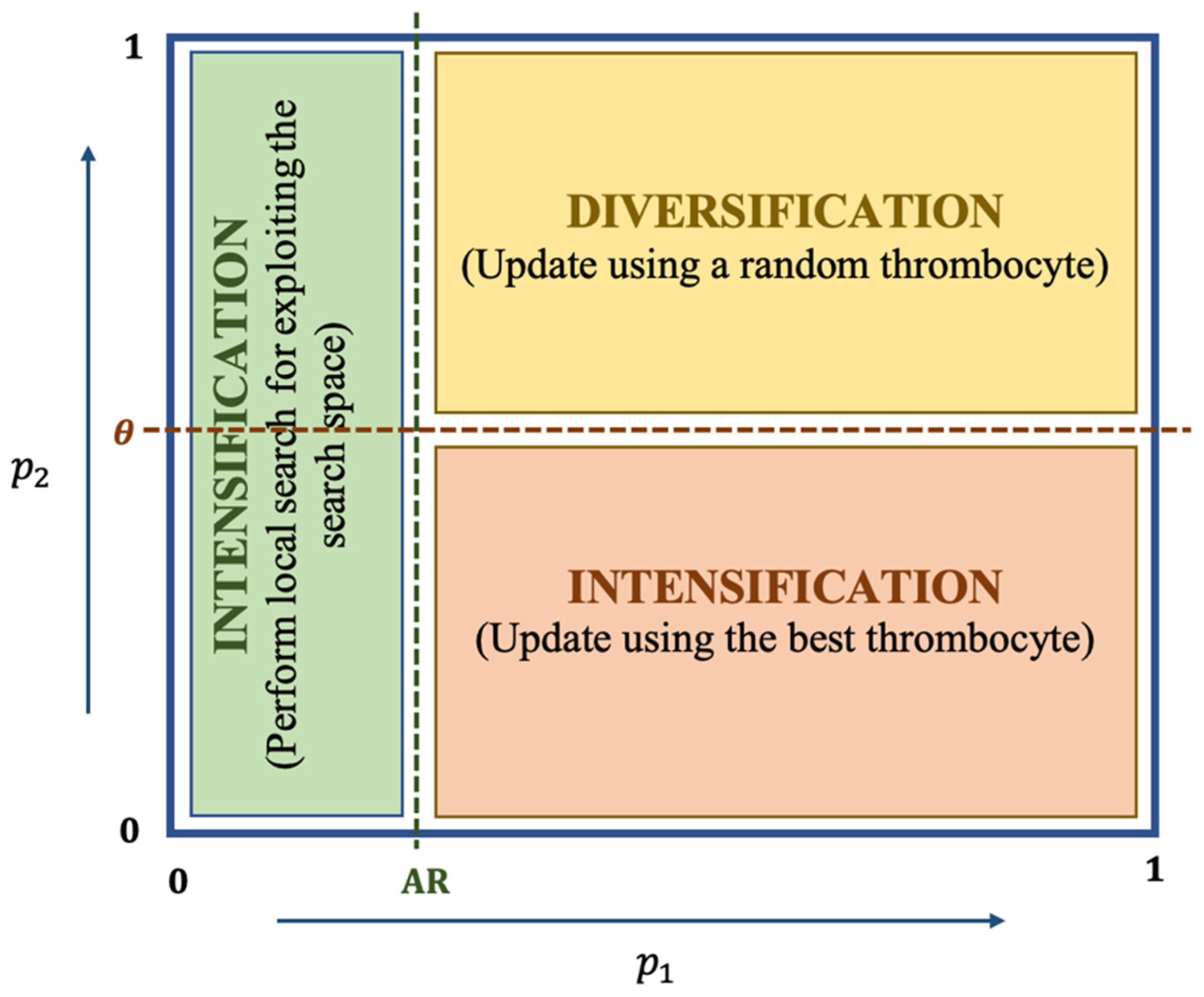
Figure 2 shows all the updating phases of BCA. For updating the positions of the thrombocytes, we use AR, i.e., Activation rate. After an injury, thrombocytes get activated by the chemicals released from the site of injury. If the thrombocytes are not fully activated, the coagulation process becomes slow. On the other hand, once the thrombocytes get activated, they update their positions either based on some random thrombocyte or the best thrombocyte. In this case, there is a high probability that we achieve fast convergence towards the global optimum. Moreover, once the thrombocytes are activated, there are high chances that they remain activated throughout the coagulation process. Hence, we use a lower value of AR and set AR = 0.1 in this work. We use a uniformly distributed random number p₁ in the range [0, 1] for comparing with the activation rate AR.

Once p₁ > AR, the thrombocytes are activated and are ready to encounter some change in their positions. We can update the positions based on either diversification (exploration) or intensification (exploitation) as discussed below:

Diversification or Exploration

Once the concentration of the procoagulants surpasses the threshold ($\theta$), rapid thrombin production is observed. This is achieved by the migration of a large number of thrombocytes to the site of injury. We use a uniformly distributed random number $p_2$ in the range [0, 1] for comparing with the threshold $\theta$. Once $p_1$ > AR and $p_2$ > $\theta$, the thrombocytes migrate and update their positions. The thrombocytes propagate in a random fashion based on the position of other thrombocytes. In the diversification phase, we update the position of a thrombocyte based on another thrombocyte selected randomly from the population. Thus, $(p_1$ > AR) $\wedge (p_2$ > $\theta )$ emphasize diversification and permit the BCA to accomplish a global search. The mathematical model is as follows:

$$d=\left|C{\mathit{x}}_{rand}\left(t\right)-\mathit{x}\left(t\right)\right|$$

(5)

$$\mathit{x}\left(t+1\right)={\mathit{x}}_{rand}\left(t\right)-P_{f}d$$

(6)

Note that ${\mathit{x}}_{rand}\left(t\right)$ in Equations (5) and (6) are the same values, i.e., we do not sample twice. Here, $C$ is a coefficient and arbitrarily taken as $C=2r_1$ where $r_1$ is a uniformly distributed random number in [0, 1]. We introduce the Propagation factor ($P_f$) which is indeed a scaling parameter used to govern the step sizes of the random walks. This parameter controls the strength of the randomness in BCA. In order to speed up the overall convergence, the perturbation should be reduced gradually. Hence, the value of $P_f$ is reduced adaptively at each iteration using the reduction formulation as follows:

$$P_f\left(t\right)=2\left(1-\frac{t}{Max\_iter}\right), for t=1, 2, 3,\dots , Max\_iter$$

(7)

The parameters $P_f$ and $C$ are responsible for better diversification and intensification over the course of iterations.

Intensification or Exploitation

The condition $(p_1$ > AR) $\wedge (p_2\le$ $\theta )$ emphasizes a local search and exploitation of the search space. In this case, the best thrombocyte position is found, and all the other thrombocytes update their positions depending on their distances from the best thrombocyte. Mathematically, we express this behavior by the following equations:

$$d_{best}=\left|{\mathit{x}}^{*}\left(t\right)-\mathit{x}\left(t\right)\right|$$

(8)

$$\mathit{x}\left(t+1\right)={\mathit{x}}^{*}\left(t\right)-{\mathit{x}}^{\prime }$$

(9)

where, ${\mathit{x}}^{\prime }=P_f\mathit{x}\left(t\right)+C{d}_{best}.$

It is important to note that we update ${\mathit{x}}^{*}$ in each iteration if a better solution is found. The best candidate solution in each iteration is considered as the best obtained solution or nearly the optimum so far. Also, we can observe (from Equation (9)) that any thrombocyte can update its position around the proximity of the current best thrombocyte (best thrombocyte obtained so far). Therefore, BCA allows good intensification (i.e., exploitation) of the search space. Also, we assume that there is a 50% probability to select between either the diversification or the intensification for updating the position of the thrombocytes during optimization. Hence, we choose $\theta =0.5$ in this work. We observe that depending on the value of $p_2,$ BCA permits to switch efficiently between diversification and intensification.

When $p_1\le$ AR, the thrombocytes are not yet fully activated and are not ready for the propagation phase (i.e., production of thrombin). We assume that the thrombocytes are partially activated and form a thrombocyte (platelet) plug responsible for primary hemostasis. (Instantly after an injury, the thrombocytes immediately form a plug at the site of injury; this is called primary hemostasis.) We update the positions of the thrombocytes based on the current best thrombocyte, i.e., exploiting the search space. This is mathematically formulated as follows:

$$\mathit{x}\left(t+1\right)={\mathit{x}}^{*}\left(t\right)-k{P}_{f}d\prime$$

(10)

where $d\prime =\left|C{\mathit{x}}^{*}\left(t\right)-\mathit{x}\left(t\right)\right|$ and $k=P_f\left(C-1\right)$.

2.2.3. Termination Phase

The updating phase persists until the termination (i.e., stopping) criteria is not reached. We can define the termination condition in a number of ways: tolerance limit (a specific value of error rate is attained), $Max\_iter$ completed, no improvement in the fitness after the maximum number of iterations, or another suitable condition. In this work, we consider the maximum number of iterations (i.e., $Max\_iter$) reached as the stopping criteria. Once the updating phase is over, the termination phase initiates, and the termination criteria is checked. BCA outputs the best solution (i.e., thrombocyte position) and the corresponding best fitness value.

2.3. Pseudocode of BCA

The aforesaid three phases make up the whole structure of BCA. This modeling is utilized to propose the new algorithm as exemplified in Algorithm 1 which explains the pseudo code of BCA.

Algorithm 1. Pseudo-code of Blood Coagulation Algorithm (BCA)

begin

Objective function $f\left(\mathit{x}\right), \mathit{x}=\left(x_1,x_2, ....x_n\right)$, n = number of dimensions

Initialize BCA parameters   ● $\mathrm{Choose} \mathrm{the} \mathrm{number} \mathrm{of} \mathrm{solutions}/\mathrm{thrombocyte} (\mathrm{i}.\mathrm{e}., N_{Pop}$ = Population size)   ● $\mathrm{Set} \mathrm{the} \mathrm{maximum} \mathrm{number} \mathrm{of} \mathrm{iterations} (\mathrm{i}.\mathrm{e}., Max\_iter$)   ● $\mathrm{Define} \mathrm{the} \mathrm{Activation} \mathrm{Rate} \left(\mathrm{AR}\right), \mathrm{Threshold} (\theta$)

Initialize randomly a population of solutions between LB and UB

Calculate the cost (fitness) of initial solutions

${\mathit{x}}^{*}$ = The best thrombocyte position (i.e., solution)

while (t < $Max\_iter$) do

for (each thrombocyte (${\mathit{x}}_i$)) do

Update $P_f$ (i.e., Propagation factor), $C$, $p_1$, $p_2$

if ($p_1$ > AR) then

if ($p_2$ > $\theta$) then

Select a random thrombocyte, ${\mathit{x}}_{rand}$

Update the position of the current thrombocyte by Equation (6)

else if ($p_{2 }\le$ $\theta$) then

Update the position of the current thrombocyte by Equation (9)

end if

else if ($p_1\le$ AR) then

Update the position of the current thrombocyte by Equation (10)

end if

end for

Check if any thrombocyte violates the boundary and adjust it

Evaluate the fitness of each thrombocyte

Update ${\mathit{x}}^{*}$ if better solution is found

Update iteration counter t ← t + 1

end while

return${\mathit{x}}^{*}$ (the best solution/thrombocyte position)

end

2.4. Computational Complexity

2.4.1. Time Complexity

In general, the time complexity analysis of meta-heuristic algorithms depends on the analysis of the following three processes [47]: initialization of the population, fitness evaluation, and updating of the search agents (in our case, the search agents are thrombocytes). Based on these three components, the time complexity analysis of the proposed meta-heuristic algorithm is as follows: With the thrombocytes’ population size of $N_{Pop}$, the time complexity of the initialization of BCA population is $O\left(N_{Pop}\times n\right)$ where $n$ indicates the number of dimensions (i.e., design variables) of the test function of the considered optimization problem. $O\left(T\right)$ is the time complexity of evaluating the fitness value (i.e., objective function value). Therefore, the time complexity of initial fitness evaluation is bounded by $O\left(N_{Pop}\times O\left(T\right)\right)$. Also, the computational complexity of the main loop (i.e., fitness evaluation and updating mechanism) is $O\left(Max\_iter\times N_{Pop}\times \left(n+O\left(T\right)\right)\right)$. On the basis of this analysis, we can say that the proposed BCA (as summarized in Algorithm 1) is a stochastic optimization method with polynomial time complexity.

2.4.2. Space Complexity

The space complexity of the proposed BCA quantifies the maximum amount of space required at any time instance as considered during initialization of the algorithm. Therefore, the total space complexity of BCA is $O\left(Max\_iter\times n\right)$ where $Max\_iter$ is the maximum number of iterations and $n$ defines the dimensionality of the objective function.

3. Optimization Testbed and Experimental Platform

3.1. Benchmark Set

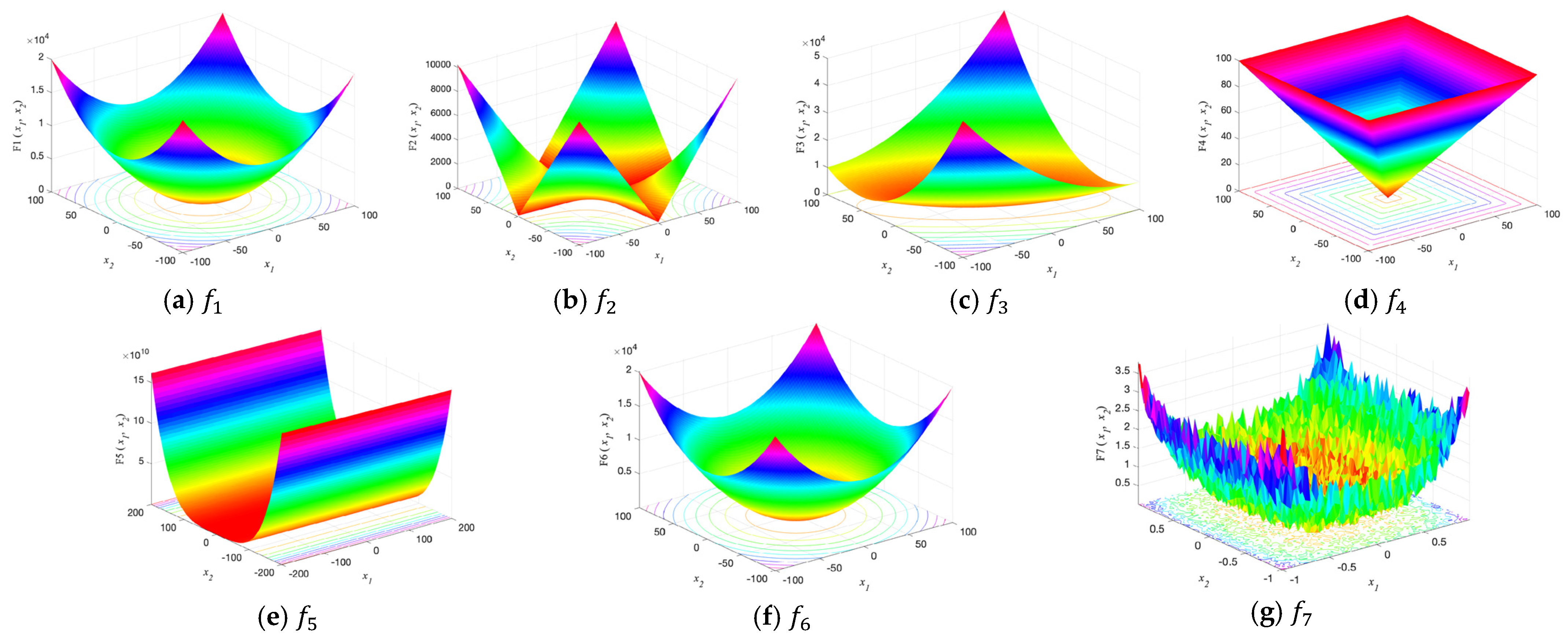
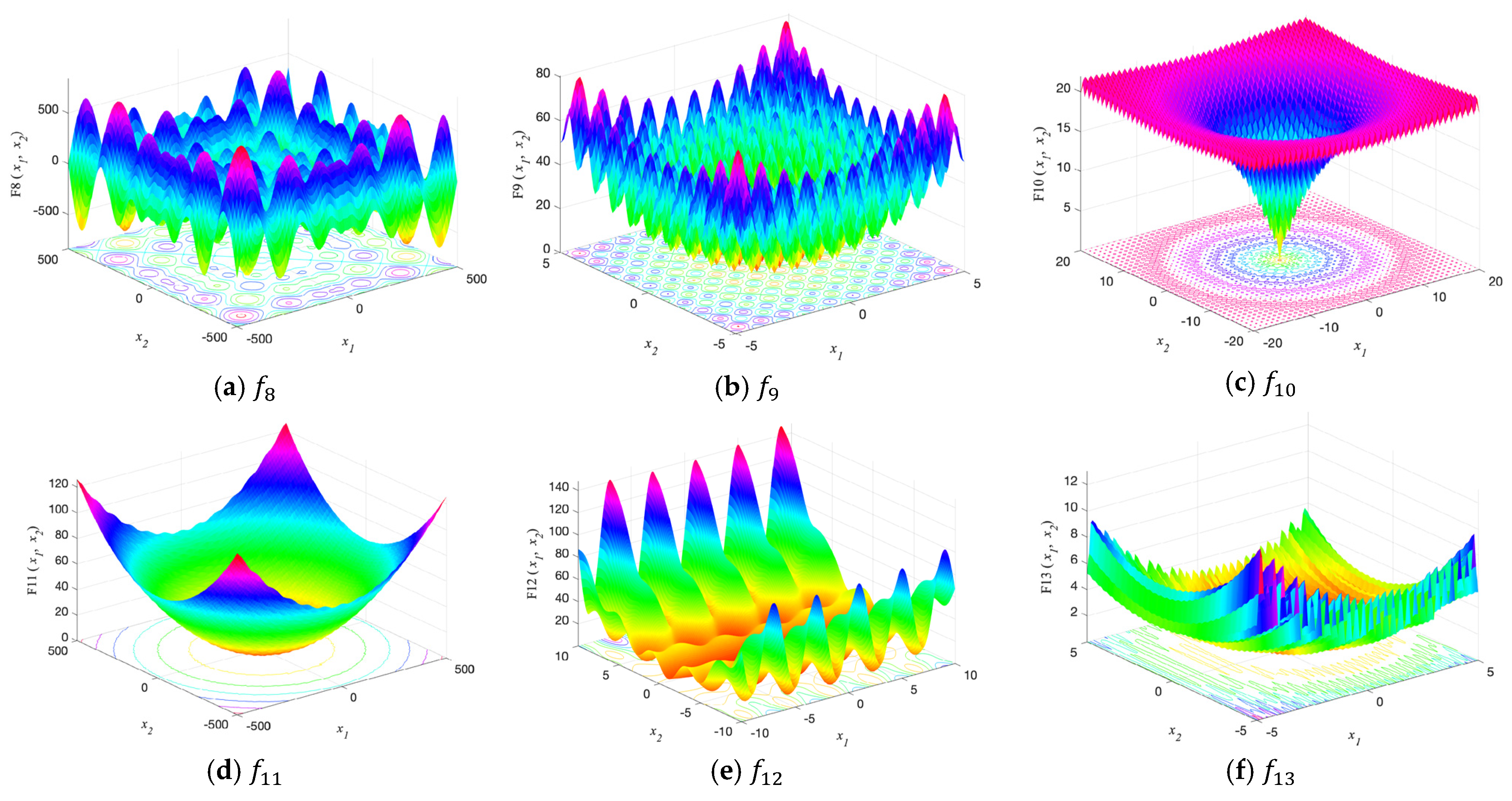
In order to investigate the efficacy and versatility of the proposed BCA optimizer, we benchmark its performance on a set of mathematical functions with known global optima. For this, we consider a well-studied set of diverse benchmark functions from the literature as the optimization test bed. The comprehensive test suite of benchmark functions consists of the following two types of functions:

• Unimodal benchmark functions: The unimodal functions have a unique global best. Since they do not have local optima, they reveal the intensification (exploitation). These functions are suitable for exploring the convergence behavior and the intensifying strength of the proposed algorithm. The unimodal functions unimodal ($f_1$ to $f_7$) considered in this work are listed in

  Table 3. List of Benchmark functions.

  Function Type	Function	Mathematical Description	Dim	Range	${\mathit{f}}_{\mathit{m}\mathit{i}\mathit{n}}$
  Unimodal	$f_1$	$f_1\left(x\right)={{\displaystyle \sum }}_{i=1}^n{x}_i^2$	30	[−100, 100]	0
  	$f_2$	$f_2\left(x\right)={{\displaystyle \sum }}_{i=1}^n\left|x_i\right|+{{\displaystyle \prod }}_{i=1}^n\left|x_i\right|$	30	[−10, 10]	0
  	$f_3$	$f_3\left(x\right)={{\displaystyle \sum }}_{i=1}^n{\left({{\displaystyle \sum }}_{j=1}^i{x}_j\right)}^2$	30	[−100, 100]	0
  	$f_4$	$f_4\left(x\right)=ma{x}_i\left\{\left|x_i\right|, 1\le i\le n\right\}$	30	[−100, 100]	0
  	$f_5$	$f_5\left(x\right)={{\displaystyle \sum }}_{i=1}^n\left[100{\left(x_{i+1}-x_i^2\right)}^2+{\left(x_i-1\right)}^2\right]$	30	[−30, 30]	0
  	$f_6$	$f_6\left(x\right)={{\displaystyle \sum }}_{i=1}^n{\left(\left[x_i+0.5\right]\right)}^2$	30	[−100, 100]	0
  	$f_7$	$f_7\left(x\right)={{\displaystyle \sum }}_{i=1}^{n}i{x}_i^4+random\left[0,1\right)$	30	[−1.28, 1.28]	0
  Multimodal	$f_8$	$f_8\left(x\right)={{\displaystyle \sum }}_{i=1}^n-x_{i}sinsin \left(\sqrt{\left|x_i\right|}\right)$	30	[500, 500]	$-418.982\times n$
  	$f_9$	$f_9\left(x\right)={{\displaystyle \sum }}_{i=1}^n\left[x_i^2-10coscos \left(2\pi x_i\right)+10\right]$	30	[−5.12, 5.12]	0
  	$f_{10}$	$f_{10}\left(x\right)=-20exp\left(-0.2\sqrt{\frac{1}{n}{{\displaystyle \sum }}_{i=1}^n{x}_i^2}\right)-exp\left(\frac{1}{n}{{\displaystyle \sum }}_{i=1}^{n}coscos \left(2\pi x_i\right) \right)+20+e$	30	[−32, 32]	0
  	$f_{11}$	$f_{11}\left(x\right)=\frac{1}{4000}{{\displaystyle \sum }}_{i=1}^n{x}_i^2-{{\displaystyle \prod }}_{i=1}^{n}coscos \left(\frac{x_i}{\sqrt{i}}\right)+1$	30	[−600, 600]	0
  	$f_{12}$	$f_{12}\left(x\right)=\frac{\pi }{n}\left\{10sinsin \left(\pi y_1\right)+{{\displaystyle \sum }}_{i=1}^n{\left(y_i-1\right)}^2\left[1+10si{n}^2\left(\pi y_{i+1}\right)\right]+{\left(y_n-1\right)}^2\right\}+{{\displaystyle \sum }}_{i=1}^{n}u\left(x_i, 10, 100, 4\right)$ $y_i=1+\frac{x_i+1}{4}u\left(x_i, a,k,m\right)=k{\left(x_i-a\right)}^m, x_i>a 0,-a<x_i<a k{\left(-x_i-a\right)}^m, x_i<-a$	30	[−50, 50]	0
  	$f_{13}$	$f_{13}\left(x\right)=0.1\left\{si{n}^2\left(3\pi x_1\right)+{{\displaystyle \sum }}_{i=1}^n{\left(x_i-1\right)}^2\left[1+si{n}^2\left(3\pi x_i+1\right)\right]+{\left(x_n-1\right)}^2\left[1+si{n}^2\left(2\pi x_n\right)\right]\right\}+{{\displaystyle \sum }}_{i=1}^{n}u\left(x_i, 5, 100, 4\right)$	30	[−50, 50]	0
  Fixed-dimension Multimodal	$f_{14}$	$f_{14}\left(x\right)={\left(\frac{1}{500}+{{\displaystyle \sum }}_{j=1}^{25}\frac{1}{j+{{\displaystyle \sum }}_{i=1}^2{\left(x_i-a_{ij}\right)}^6}\right)}^{-1}$	2	[−65, 65]	1
  	$f_{15}$	$f_{15}\left(x\right)={{\displaystyle \sum }}_{i=1}^{11}{\left[a_i-\frac{x_1\left(b_i^2+b_i{x}_2\right)}{b_i^2+b_i{x}_3+x_4}\right]}^2$	4	[−5, 5]	0.00030
  	$f_{16}$	$f_{16}\left(x\right)=4x_1^2-2.1x_1^4+\frac{1}{3}{x}_1^6+x_1{x}_2-4x_2^2+4x_2^4$	2	[−5, 5]	−1.0316
  	$f_{17}$	$f_{17}\left(x\right)={\left(x_2-\frac{5.1}{4{\pi }^2}{x}_1^2+\frac{5}{\pi }{x}_1-6\right)}^2+10\left(1-\frac{1}{8\pi }\right)coscos x_1+10$	2	[−5, 5]	0.398
  	$f_{18}$	$f_{18}\left(x\right)=\left[1+{\left(x_1+x_2+1\right)}^2\left(19-14x_1+3x_1^2-14x_2+6x_1{x}_2+3x_2^2\right)\right]\left[30+{\left(2x_1-3x_2\right)}^2\left(18-32x_1+12x_1^2+48x_2-36x_1{x}_2+27x_2^2\right)\right]$	2	[−2, 2]	3
  	$f_{19}$	$f_{19}\left(x\right)=-{{\displaystyle \sum }}_{i=1}^4{c}_i exp\left({{\displaystyle \sum }}_{j=1}^3{a}_{ij}{\left(x_j-p_{ij}\right)}^2\right)$	3	[1, 3]	−3.86
  	$f_{20}$	$f_{20}\left(x\right)=-{{\displaystyle \sum }}_{i=1}^4{c}_i exp\left({{\displaystyle \sum }}_{j=1}^6{a}_{ij}{\left(x_j-p_{ij}\right)}^2\right)$	6	[0, 1]	−3.32
  	$f_{21}$	$f_{21}\left(x\right)=-{{\displaystyle \sum }}_{i=1}^5{\left[\left(X-a_i\right){\left(X-a_i\right)}^T+c_i\right]}^{-1}$	4	[0, 10]	−10.1532
  	$f_{22}$	$f_{22}\left(x\right)=-{{\displaystyle \sum }}_{i=1}^7{\left[\left(X-a_i\right){\left(X-a_i\right)}^T+c_i\right]}^{-1}$	4	[0, 10]	−10.4028
  	$f_{23}$	$f_{23}\left(x\right)=-{{\displaystyle \sum }}_{i=1}^{10}{\left[\left(X-a_i\right){\left(X-a_i\right)}^T+c_i\right]}^{-1}$	4	[0, 10]	−10.5363

  Note: Dim = the dimensionality of the search space (i.e., number of variables); Range = the boundary of the search space [Lower Bound, Upper Bound]; $f_{min}$ = global optimum.

  along with their mathematical definitions;
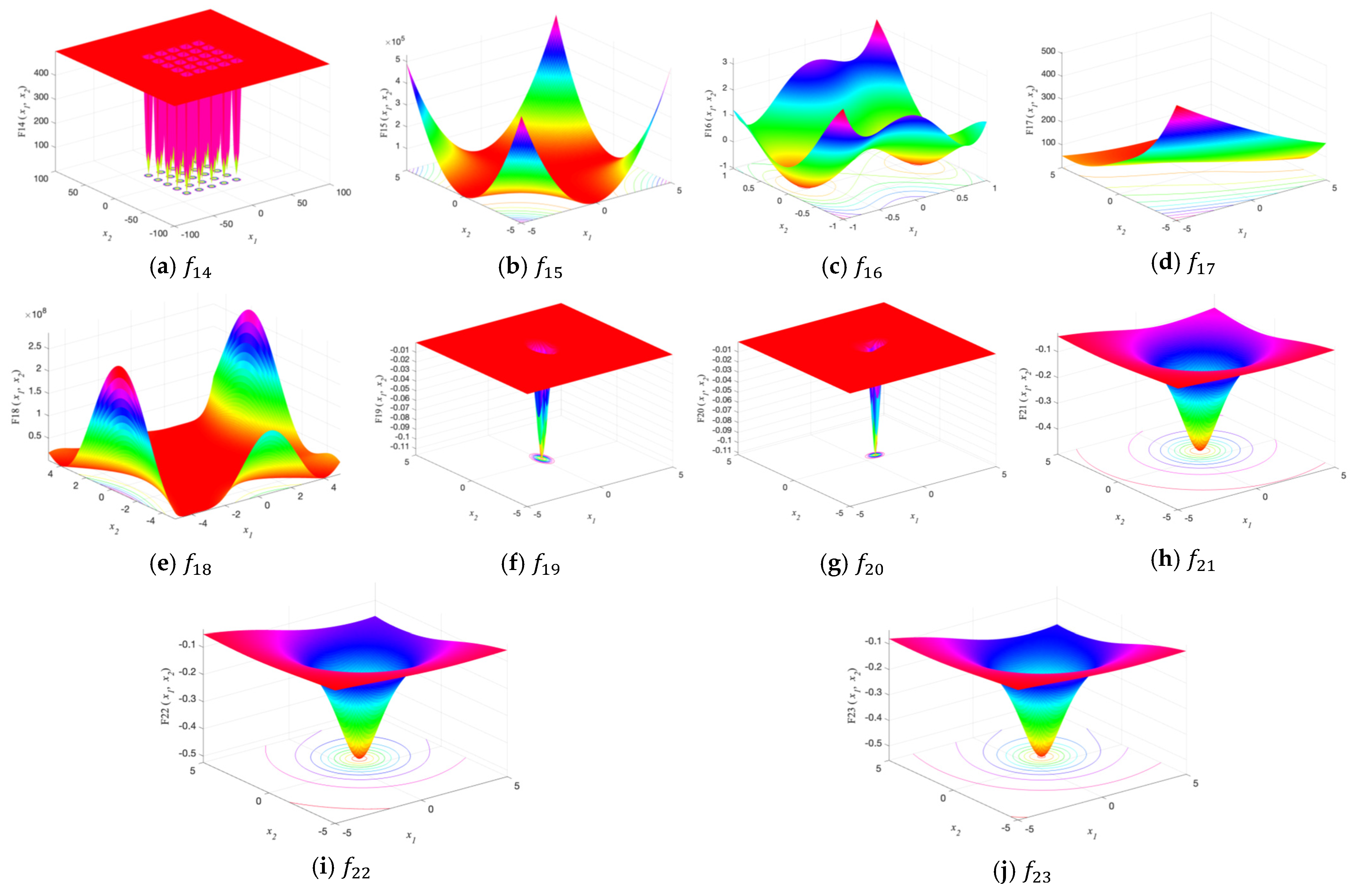
• Multimodal benchmark functions: These functions may have many local optima. Hence, the optimizer should be able to avoid stagnation around the local optimum for reaching the global optima. Therefore, these functions can unveil the diversification (or exploratory) capability of BCA and its ability to escape the local optima. The multimodal functions ($f_8$ to $f_{13}$) along with their details are presented in Table 3. It is also worth mentioning here that that fixed-dimension multimodal functions ($f_{14}$ to $f_{23}$) are also considered in this work.

The search landscape of the objective functions i.e., unimodal ($f_1$ to $f_7$), multimodal ($f_8$ to $f_{13}$), and fixed-dimension multimodal ($f_{14}$ to $f_{23}$) functions are illustrated in Figure 3, Figure 4 and Figure 5, respectively.

3.2. Experimental Setup

The proposed algorithm is implemented in MATLAB^® (R2020b) programming platform. Our experiments are performed on a system with an Apple M1 chip and 16 GB RAM, running macOS Big Sur. In each run, the maximum number of iterations (Max_iter) is chosen as the termination criterion of BCA. The value of Max_iter is set to 1000. Also, the population size is taken as 30. The activation rate and threshold are set to 0.1 and 0.5, respectively. For generating meaningful (significant) statistical results and reducing statistical errors, we repeat the simulations for each function for 30 independent runs. Additionally, we record the mean (average fitness value) and standard deviation (SD) of BCA for each benchmark function.

In order to manifest the adeptness of the proposed BCA on the benchmark test functions, we compare its performance with other well-regarded nature-inspired meta-heuristic algorithms. For this purpose, we construct a suite of 12 state-of-the-art optimizers as listed in

Table 4. Parameter settings of various algorithms.

Algorithm	Parameter	Value
# (For all algorithms)	Population size	30
	Maximum number of iterations	1000
DE [48]	Scaling factor	0.5
	Crossover probability	0.5
PSO [8]	Topology	fully connected
	Inertia factor	Linear reduction from 0.9 to 0.1
	$c_1$	2
	$c_2$	2
	Velocity limit	10% of dimension range
GA [49]	Type	Real coded
	Selection	Roulette wheel (Proportionate)
	Crossover	Whole arithmetic (Probability 0.8)
	Mutation	Gaussian (Probability 0.05)
CS [13]	$\mathrm{Discovery} \mathrm{rate} \mathrm{of} \mathrm{alien} \mathrm{solutions} (p_a$)	0.25
GWO [9]	$\mathrm{Convergence} \mathrm{parameter} (a$)	Linear reduction from 2 to 0
MFO [14]	$\mathrm{Convergence} \mathrm{constant} \left(a\right)$	[−2 −1]
	$\mathrm{Spiral} \mathrm{factor} \left(b\right)$	1
FPA [15]	$\mathrm{Probability} \mathrm{switch} \left(p\right)$	0.8
FA [16]	$\alpha$	0.5
	$\beta$	0.2
	$\gamma$	1
BAT [50]	$Q_{min}$(Minimum frequency)	0
	$Q_{max}$(Maximum frequency)	2
	$A$ (Loudness)	0.5
	$r$ (Pulse rate)	0.5
GSA [23]	Gravitational constant	100
	Alpha coefficient	20
AOA [51]	$\alpha$	5
	$\mu$	0.5
BBO [6]	Habitat modification probability	1
	Immigration probability limits	[0, 1]
	Step size	1
	Max immigration (I) and Max emigration (E)	1
	Mutation probability	0.005

. The details of parameters settings of these optimizers are also provided in Table 4. For achieving the best results, the parameters are set to the values as reported in the literature. We assume that the chosen parameters for the other methods (in Table 4) are the best possible parameters for the optimization task. To ensure a fair comparison, the population size and the maximum number of iterations for each optimizer is set to 30 and 1000, respectively.

Furthermore, for identifying significant differences in the results acquired by various optimizers, we also perform the non-parametric Wilcoxon statistical test [52] with 5% degree of significance, besides the experimental simulations and the basic statistical analysis.

4. Experimental Results and Discussion

For each benchmark function, we performed 30 simulations of each algorithm (including BCA and other algorithms listed in Table 4) with randomly generated populations. The statistical results (Mean and standard deviation) are reported in

Table 5. Comparison of the results obtained by BCA with other state-of-the-art meta-heuristic algorithms. The best results are kept in bold.

F	Metric	BCA	DE	PSO	GA	CS	GWO	MFO	FPA	FA	BAT	GSA	AOA	BBO
$f_1$	Mean	$\mathbf{9.80}\mathbf{\times }{\mathbf{10}}^{\mathbf{-}\mathbf{28}}$	$1.33\times {10}^{-3}$	$1.83\times {10}^4$	$1.03\times {10}^3$	$9.06\times {10}^{-4}$	$1.18\times {10}^{-27}$	$1.01\times {10}^3$	$2.01\times {10}^3$	$7.11\times {10}^{-3}$	$6.59\times {10}^4$	$6.08\times {10}^2$	$6.67\times {10}^{-7}$	$7.59\times {10}^1$
	SD	$1.70\times {10}^{-22}$	$5.92\times {10}^{-4}$	$3.01\times {10}^3$	$5.79\times {10}^2$	$4.55\times {10}^{-4}$	$1.47\times {10}^{-27}$	$3.05\times {10}^3$	$5.60\times {10}^2$	$3.21\times {10}^{-3}$	$7.51\times {10}^3$	$4.64\times {10}^2$	$7.45\times {10}^{-7}$	$2.75\times {10}^1$
$f_2$	Mean	$\mathbf{8.91}\mathbf{\times }{\mathbf{10}}^{\mathbf{-}\mathbf{17}}$	$6.83\times {10}^{-3}$	$3.58\times {10}^2$	$2.47\times {10}^1$	$1.49\times {10}^{-1}$	$9.71\times {10}^{-17}$	$3.19\times {10}^1$	$3.22\times {10}^1$	$4.34\times {10}^{-1}$	$2.71\times {10}^8$	$2.27\times {10}^1$	0.01	$1.36\times {10}^{-3}$
	SD	$1.3\times {10}^{-11}$	$2.06\times {10}^{-3}$	$1.35\times {10}^3$	5.68	$2.79\times {10}^{-2}$	$5.60\times {10}^{-17}$	$2.06\times {10}^1$	5.55	$1.84\times {10}^{-1}$	$1.30\times {10}^9$	3.36	0.00	$7.45\times {10}^{-3}$
$f_3$	Mean	$\mathbf{7.63}\mathbf{\times }{\mathbf{10}}^{\mathbf{-}\mathbf{16}}$	$3.97\times {10}^4$	$4.05\times {10}^4$	$2.65\times {10}^4$	$2.10\times {10}^{-1}$	$5.12\times {10}^{-5}$	$2.43\times {10}^4$	$1.41\times {10}^3$	$1.66\times {10}^3$	$1.38\times {10}^5$	$1.35\times {10}^5$	$6.87\times {10}^{-6}$	$1.21\times {10}^4$
	SD	$2.46\times {10}^{-15}$	$5.37\times {10}^3$	$8.21\times {10}^3$	$3\times {10}^3$	$5.69\times {10}^{-2}$	$2.03\times {10}^{-4}$	$1.41\times {10}^4$	$5.59\times {10}^2$	$6.72\times {10}^2$	$4.72\times {10}^4$	$4.86\times {10}^4$	$6.87\times {10}^{-6}$	$2.69\times {10}^3$
$f_4$	Mean	$\mathbf{7.01}\mathbf{\times }{\mathbf{10}}^{\mathbf{-}\mathbf{10}}$	$1.15\times {10}^1$	$4.39\times {10}^1$	$5.17\times {10}^1$	$9.65\times {10}^{-2}$	$1.24\times {10}^{-6}$	$7.00\times {10}^1$	$2.38\times {10}^1$	$1.11\times {10}^{-1}$	$8.51\times {10}^1$	$7.87\times {10}^1$	$1.40\times {10}^{-3}$	$3.02\times {10}^1$
	SD	$1.77\times {10}^{-9}$	2.37	3.64	$1.05\times {10}^1$	$1.94\times {10}^{-2}$	$1.94\times {10}^{-6}$	7.06	2.77	$4.75\times {10}^{-2}$	2.95	2.81	$1.90\times {10}^{-3}$	4.39
$f_5$	Mean	3.72	$1.06\times {10}^2$	$1.96\times {10}^7$	$1.95\times {10}^4$	$2.76\times {10}^1$	$2.70\times {10}^1$	$7.35\times {10}^3$	$3.17\times {10}^5$	$7.97\times {10}^1$	$2.10\times {10}^8$	$7.41\times {10}^2$	$2.49\times {10}^1$	$1.82\times {10}^3$
	SD	8.72	$1.01\times {10}^2$	$6.25\times {10}^6$	$1.31\times {10}^4$	$4.51\times {10}^{-1}$	$7.78\times {10}^{-1}$	$2.26\times {10}^4$	$1.75\times {10}^5$	$7.39\times {10}^1$	$4.17\times {10}^7$	$7.81\times {10}^2$	$3.64\times {10}^{-1}$	$9.40\times {10}^2$
$f_6$	Mean	$1.36\times {10}^{-2}$	$1.44\times {10}^{-3}$	$1.87\times {10}^4$	$9.01\times {10}^2$	$3.13\times {10}^{-3}$	$8.44\times {10}^{-1}$	$2.68\times {10}^3$	$1.70\times {10}^3$	$6.94\times {10}^{-3}$	$6.69\times {10}^4$	$3.08\times {10}^3$	$\mathbf{3.47}\mathbf{\times }{\mathbf{10}}^{\mathbf{-}\mathbf{4}}$	$6.71\times {10}^1$
	SD	$9.83\times {10}^{-3}$	$5.38\times {10}^{-4}$	$2.92\times {10}^3$	$2.84\times {10}^2$	$1.30\times {10}^{-3}$	$3.18\times {10}^{-1}$	$5.84\times {10}^3$	$3.13\times {10}^2$	$3.61\times {10}^{-3}$	$5.87\times {10}^3$	$8.98\times {10}^2$	$3.47\times {10}^{-4}$	$2.20\times {10}^1$
$f_7$	Mean	$3.95\times {10}^{-4}$	$5.24\times {10}^{-2}$	$1.07\times {10}^1$	$1.91\times {10}^{-1}$	$7.29\times {10}^{-2}$	$1.70\times {10}^{-3}$	4.50	$3.41\times {10}^{-1}$	$6.62\times {10}^{-2}$	$4.57\times {10}^1$	$1.12\times {10}^{-1}$	$\mathbf{3.92}\mathbf{\times }{\mathbf{10}}^{\mathbf{-}\mathbf{6}}$	$2.91\times {10}^{-3}$
	SD	$4.78\times {10}^{-4}$	$1.37\times {10}^{-2}$	3.05	$1.50\times {10}^{-1}$	$2.21\times {10}^{-2}$	$1.06\times {10}^{-3}$	9.21	$1.10\times {10}^{-1}$	$4.23\times {10}^{-2}$	7.82	$3.76\times {10}^{-2}$	$3.92\times {10}^{-6}$	$1.83\times {10}^{-3}$
$f_8$	Mean	$\mathbf{-}\mathbf{1.25}\mathbf{\times }{\mathbf{10}}^{\mathbf{4}}$	$-6.82\times {10}^3$	$-3.86\times {10}^3$	$-1.26\times {10}^4$	$-5.19\times {10}^{19}$	$-5.97\times {10}^3$	$-8.48\times {10}^3$	$-6.45\times {10}^3$	$-5.85\times {10}^3$	$-2.33\times {10}^3$	$-2.35\times {10}^3$	$-1.22\times {10}^4$	$-1.24\times {10}^4$
	SD	$4.30\times {10}^1$	$3.94\times {10}^2$	$2.49\times {10}^2$	4.51	$1.76\times {10}^{20}$	$7.10\times {10}^2$	$7.98\times {10}^2$	$3.03\times {10}^2$	$1.16\times {10}^3$	$2.96\times {10}^2$	$3.82\times {10}^2$	$1.22\times {10}^3$	$3.50\times {10}^1$
$f_9$	Mean	$\mathbf{1.70}\mathbf{\times }{\mathbf{10}}^{\mathbf{-}\mathbf{14}}$	$1.58\times {10}^2$	$2.87\times {10}^2$	9.04	$1.51\times {10}^1$	2.19	$1.59\times {10}^2$	$1.82\times {10}^2$	$3.82\times {10}^1$	$1.92\times {10}^2$	$3.10\times {10}^1$	$3.42\times {10}^{-7}$	0.01
	SD	$3.04\times {10}^{-14}$	$1.17\times {10}^1$	$1.95\times {10}^1$	4.58	1.25	3.69	$3.21\times {10}^1$	$1.24\times {10}^1$	$1.12\times {10}^1$	$3.56\times {10}^1$	$1.36\times {10}^1$	$3.42\times {10}^{-7}$	0.00
$f_{10}$	Mean	$\mathbf{8.88}\mathbf{\times }{\mathbf{10}}^{\mathbf{-}\mathbf{16}}$	$1.21\times {10}^{-2}$	$1.75\times {10}^1$	$1.36\times {10}^1$	$3.29\times {10}^{-2}$	$1.03\times {10}^{-13}$	$1.74\times {10}^1$	7.14	$4.58\times {10}^{-2}$	$1.92\times {10}^1$	3.74	$\mathbf{8.88}\mathbf{\times }{\mathbf{10}}^{\mathbf{-}\mathbf{16}}$	2.13
	SD	$2.89\times {10}^{-11}$	$3.30\times {10}^{-3}$	$3.67\times {10}^1$	1.51	$7.93\times {10}^{-3}$	$1.70\times {10}^{-14}$	4.95	1.08	$1.20\times {10}^{-2}$	$2.43\times {10}^{-1}$	$1.71\times {10}^{-1}$	$8.88\times {10}^{-16}$	$3.53\times {10}^{-1}$
$f_{11}$	Mean	$\mathbf{3.49}\mathbf{\times }{\mathbf{10}}^{\mathbf{-}\mathbf{15}}$	$3.52\times {10}^{-2}$	$1.70\times {10}^2$	$1.01\times {10}^1$	$4.29\times {10}^{-5}$	$4.76\times {10}^{-3}$	$3.10\times {10}^1$	$1.73\times {10}^1$	$4.23\times {10}^{-3}$	$6.01\times {10}^2$	$4.86\times {10}^{-1}$	$1.00\times {10}^{-6}$	1.46
	SD	$1.86\times {10}^{-14}$	$7.20\times {10}^{-2}$	$3.17\times {10}^1$	2.43	$2.00\times {10}^{-5}$	$8.57$	$5.94\times {10}^1$	3.63	$1.29\times {10}^{-3}$	$5.50$	$4.97\times {10}^{-2}$	$1.21\times {10}^6$	$1.69\times {10}^{-1}$
$f_{12}$	Mean	$\mathbf{4.19}\mathbf{\times }{\mathbf{10}}^{\mathbf{-}\mathbf{6}}$	$2.25\times {10}^{-3}$	$1.51\times {10}^7$	4.77	$5.57\times {10}^{-5}$	$4.83\times {10}^{-2}$	$2.46\times {10}^2$	$3.05\times {10}^2$	$3.13\times {10}^{-4}$	$4.71\times {10}^8$	$4.63\times {10}^{-1}$	$4.28\times {10}^{-6}$	$6.68\times {10}^{-1}$
	SD	$5.43\times {10}^{-4}$	$1.70\times {10}^{-3}$	$9.88\times {10}^6$	1.56	$4.96\times {10}^{-5}$	$2.12\times {10}^{-2}$	$1.21\times {10}^3$	$1.04\times {10}^3$	$1.76\times {10}^{-4}$	$1.54\times {10}^8$	$1.37\times {10}^{-1}$	$4.28\times {10}^{-6}$	$2.62\times {10}^{-1}$
$f_{13}$	Mean	$\mathbf{1.99}\mathbf{\times }{\mathbf{10}}^{\mathbf{-}\mathbf{3}}$	$9.12\times {10}^{-3}$	$5.73\times {10}^7$	$1.52\times {10}^1$	$8.19\times {10}^{-3}$	$5.96\times {10}^{-1}$	$2.73\times {10}^7$	$9.59\times {10}^4$	$2.08\times {10}^{-3}$	$9.40\times {10}^8$	7.61	$3.10\times {10}^{-1}$	1.82
	SD	$5.37\times {10}^{-3}$	$1.16\times {10}^{-2}$	$2.68\times {10}^7$	4.52	$6.74\times {10}^{-3}$	$2.23\times {10}^{-1}$	$1.04\times {10}^8$	$1.46\times {10}^5$	$9.62\times {10}^{-4}$	$1.67\times {10}^8$	1.22	$3.10\times {10}^{-1}$	$3.41\times {10}^{-1}$
$f_{14}$	Mean	$\mathbf{9.98}\mathbf{\times }{\mathbf{10}}^{\mathbf{-}\mathbf{1}}$	1.23	1.39	$\mathbf{9.98}\mathbf{\times }{\mathbf{10}}^{\mathbf{-}\mathbf{1}}$	$1.27\times {10}^1$	4.17	2.74	9.98 × 10−1	3.51	$1.27\times {10}^1$	$\mathbf{9.98}\mathbf{\times }{\mathbf{10}}^{\mathbf{-}\mathbf{1}}$	$\mathbf{9.98}\mathbf{\times }{\mathbf{10}}^{\mathbf{-}\mathbf{1}}$	$\mathbf{9.98}\mathbf{\times }{\mathbf{10}}^{\mathbf{-}\mathbf{1}}$
	SD	$3.02\times {10}^{-10}$	$9.23\times {10}^{-1}$	$4.60\times {10}^{-1}$	$4.52\times {10}^{-16}$	$1.81\times {10}^{-15}$	3.61	1.82	$2.00\times {10}^{-4}$	2.16	6.96	$4.52\times {10}^{-16}$	$5.54\times {10}^{-1}$	$4.52\times {10}^{-16}$
$f_{15}$	Mean	$\mathbf{3.07}\mathbf{\times }{\mathbf{10}}^{\mathbf{-}\mathbf{4}}$	$5.63\times {10}^{-4}$	$1.61\times {10}^{-3}$	$3.33\times {10}^{-2}$	$3.13\times {10}^{-4}$	$6.24\times {10}^{-3}$	$2.35\times {10}^{-3}$	$6.88\times {10}^{-4}$	$1.01\times {10}^{-3}$	$3.00\times {10}^{-2}$	$1.03\times {10}^{-3}$	$3.12\times {10}^{-4}$	$1.66\times {10}^{-2}$
	SD	$4.59\times {10}^{-4}$	$2.81\times {10}^{-4}$	$4.60\times {10}^{-4}$	$2.70\times {10}^{-2}$	$2.99\times {10}^{-5}$	$1.25\times {10}^{-2}$	$4.92\times {10}^{-3}$	$1.55\times {10}^{-4}$	$4.01\times {10}^{-4}$	$3.33\times {10}^{-2}$	$3.66\times {10}^{-3}$	$2.64\times {10}^{-4}$	$8.60\times {10}^{-3}$
$f_{16}$	Mean	−1.03	−1.03	−1.03	$-3.78\times {10}^{-1}$	−1.03	−1.03	−1.03	−1.03	−1.03	$-6.87\times {10}^{-1}$	−1.03	−1.03	$-8.30\times {10}^{-1}$
	SD	$6.32\times {10}^{-6}$	$6.78\times {10}^{-16}$	$2.95\times {10}^{-3}$	$3.42\times {10}^{-1}$	$6.78\times {10}^{-16}$	$6.78\times {10}^{-16}$	$6.78\times {10}^{-16}$	$6.78\times {10}^{-16}$	$6.78\times {10}^{-16}$	$8.18\times {10}^{-1}$	$6.78\times {10}^{-16}$	$5.48\times {10}^{-5}$	$3.16\times {10}^{1-}$
$f_{17}$	Mean	$\mathbf{3.98}\mathbf{\times }{\mathbf{10}}^{\mathbf{-}\mathbf{1}}$	$\mathbf{3.98}\mathbf{\times }{\mathbf{10}}^{\mathbf{-}\mathbf{1}}$	$4.00\times {10}^{-1}$	$5.24\times {10}^{-1}$	$\mathbf{3.98}\mathbf{\times }{\mathbf{10}}^{\mathbf{-}\mathbf{1}}$	$\mathbf{3.98}\mathbf{\times }{\mathbf{10}}^{\mathbf{-}\mathbf{1}}$	$\mathbf{3.98}\mathbf{\times }{\mathbf{10}}^{\mathbf{-}\mathbf{1}}$	$\mathbf{3.98}\mathbf{\times }{\mathbf{10}}^{\mathbf{-}\mathbf{1}}$	$\mathbf{3.98}\mathbf{\times }{\mathbf{10}}^{\mathbf{-}\mathbf{1}}$	$\mathbf{3.98}\mathbf{\times }{\mathbf{10}}^{\mathbf{-}\mathbf{1}}$	$\mathbf{3.98}\mathbf{\times }{\mathbf{10}}^{\mathbf{-}\mathbf{1}}$	$\mathbf{3.98}\mathbf{\times }{\mathbf{10}}^{\mathbf{-}\mathbf{1}}$	$5.49\times {10}^{-1}$
	SD	$9.31\times {10}^{-5}$	$1.69\times {10}^{-16}$	$1.39\times {10}^{-3}$	$6.06\times {10}^{-2}$	$1.69\times {10}^{-16}$	$1.69\times {10}^{-16}$	$1.69\times {10}^{-16}$	$1.69\times {10}^{-16}$	$1.69\times {10}^{-16}$	$1.58\times {10}^{-3}$	$1.69\times {10}^{-16}$	$2.54\times {10}^{-6}$	$6.05\times {10}^{-2}$
$f_{18}$	Mean	3.00	3.00	3.10	3.00	3.00	3.00	3.00	3.00	3.00	$1.47\times {10}^1$	3.00	3.00	3.00
	SD	$1.28\times {10}^{-4}$	0.00	$7.60\times {10}^{-2}$	0.00	0.00	$4.07\times {10}^{-5}$	0.00	0.00	0.00	$2.21\times {10}^1$	0.00	$1.00\times {10}^{-2}$	0.00
$f_{19}$	Mean	−3.86	−3.86	−3.86	−3.42	−3.86	−3.86	−3.86	−3.86	−3.86	−3.84	−3.86	−3.86	−3.78
	SD	$3.69\times {10}^{-3}$	$3.16\times {10}^{-15}$	$1.24\times {10}^{-3}$	$3.03\times {10}^{-1}$	$3.16\times {10}^{-15}$	$3.14\times {10}^{-3}$	$1.44\times {10}^{-3}$	$3.16\times {10}^{-15}$	$3.16\times {10}^{-15}$	$1.41\times {10}^{-1}$	$3.16\times {10}^{-15}$	$4.29\times {10}^{-4}$	$1.26\times {10}^{-1}$
$f_{20}$	Mean	−3.32	−3.27	−3.11	−1.61	−3.32	−3.25	−3.23	−3.29	−3.28	−3.25	−3.24	−3.32	−2.70
	SD	$3.33\times {10}^{-1}$	$5.89\times {10}^{-2}$	$2.91\times {10}^{-2}$	$4.60\times {10}^{-1}$	$1.77\times {10}^{-15}$	$6.43\times {10}^{-2}$	$6.42\times {10}^{-2}$	$1.95\times {10}^{-2}$	$6.36\times {10}^{-2}$	$5.89\times {10}^{-2}$	$1.51\times {10}^{-1}$	$1.25\times {10}^1$	$3.57\times {10}^{-1}$
$f_{21}$	Mean	−1.01	−9.64	−4.14	−6.66	−5.05	−8.64	−6.88	−5.21	−7.67	−4.26	−8.65	−8.85	−8.31
	SD	2.00	1.51	$9.19\times {10}^{-1}$	3.73	$1.77\times {10}^{-15}$	2.56	3.18	$8.15\times {10}^{-2}$	3.50	2.55	1.77	1.25	2.88
$f_{22}$	Mean	−1.04	−9.74	−6.01	−5.58	−5.08	−1.04	−8.26	−5.34	−9.63	−5.60	$-1.02\times {10}^1$	$\mathbf{-}\mathbf{1.04}\mathbf{\times }{\mathbf{10}}^{\mathbf{1}}$	−9.38
	SD	$2.51\times {10}^{-4}$	1.98	1.96	2.60	$8.88\times {10}^{-16}$	$6.78\times {10}^{-4}$	3.07	$5.36\times {10}^{-2}$	2.29	3.02	$7.27\times {10}^{-3}$	2.21	2.59
$f_{23}$	Mean	$\mathbf{-}\mathbf{1.05}\mathbf{\times }{\mathbf{10}}^{\mathbf{1}}$	$\mathbf{-}\mathbf{1.05}\mathbf{\times }{\mathbf{10}}^{\mathbf{1}}$	−4.72	−4.69	−5.12	$-1.08\times {10}^1$	−7.65	−5.29	−9.75	−3.97	$-1.01\times {10}^1$	$\mathbf{-}\mathbf{1.05}\mathbf{\times }{\mathbf{10}}^{\mathbf{1}}$	−6.23
	SD	$2.93\times {10}^{-7}$	8.88 × 10−15	1.74	3.25	$1.77\times {10}^{-15}$	1.72	3.57	$3.56\times {10}^{-1}$	2.34	3.00	1.70	1.02	3.78

.

4.1. Intensification and Diversification Capabilities of BCA

The intensification (exploitation) capability of BCA is evaluated by using the unimodal benchmark functions ($f_1$ to $f_7$). Moreover, to test the capability of BCA to investigate different promising regions of the search space (i.e., diversification), we solve multimodal benchmark functions ($f_8$ to $f_{23}$) with many local optima. The statistical results (based on the evaluation metrics: mean and SD) reported in Table 5 prove that BCA is very competitive with other meta-heuristic algorithms. It is seen that BCA provides considerably better results than other algorithms for most of the functions, demonstrating its worthy performance.

The results presented in Table 5 indicate that the proposed BCA can acquire the best results against its competitor algorithms on $f_1-f_5$ (the unimodal test cases) and $f_8-f_{13}$ (the multimodal test cases). It is observed that the results acquired by BCA are substantially better than its competitors in handling 84.6% of the functions $f_1-f_{13}$ over 30 dimensions. This validates the superior performance of BCA over other algorithms. Also, for fixed-dimensional multimodal benchmark $f_{14}$, the results are superior and competitive. For $f_{15}$, BCA gives superior results, as can be verified from Table 5. The results on the functions $f_{16}-f_{19}$ are very competitive, and good results are acquired by most of the approaches. Thus, based on the results in Table 5, the proposed BCA has always achieved the best (high quality solutions) results on $f_{14}-f_{23}$ (fixed-dimension multimodal) test cases compared to other algorithms.

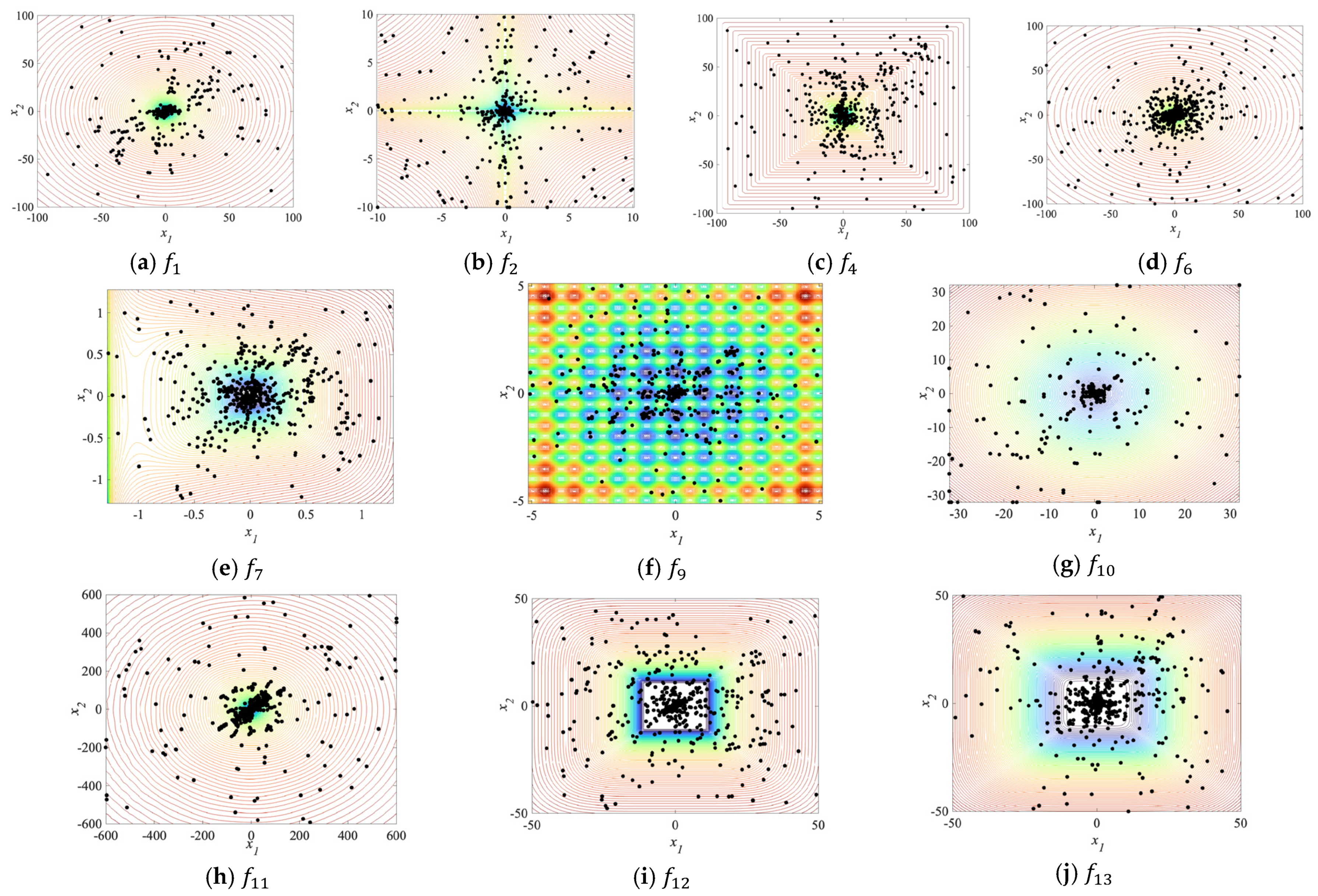
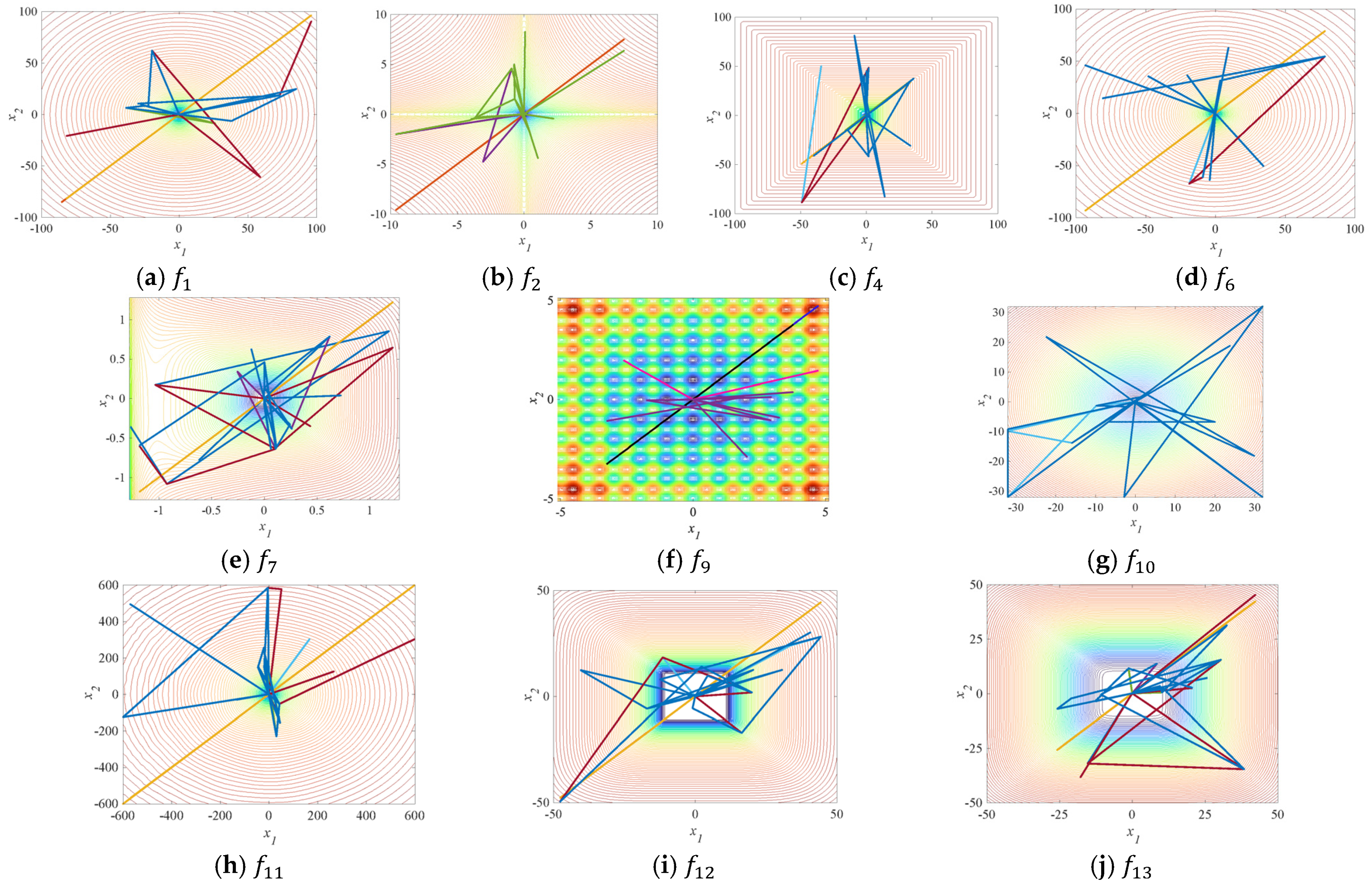
To better understand and visualize the intensification and diversification capabilities of BCA, we record the search history of the thrombocytes. Figure 6 presents the search history of thrombocytes for some of the benchmark functions. Note that we consider 2D versions of the functions for visualization of the search history (positions of thrombocytes over the course of iterations). Referring to Figure 6, the distribution of the thrombocytes indicates that BCA efficiently searches different promising regions over the search space. Further, it exploits the vicinity of the favorable regions to reach the global optimal solutions. The thrombocytes converge at the global optima and hence prove the avoidance of local optima by BCA. This can also be verified by investigating the trajectories of some randomly chosen thrombocytes (2D visualization) (Figure 7). Different colors are used to denote the trajectories of different thrombocytes. From Figure 7, it can be observed that the trajectories (zig-zag patterns) pass through different regions of the search space, thereby validating the diversification potential of BCA. These zig-zag paths, therefore, assist us to understand the searching behavior of the thrombocytes over the solution space. Moreover, the trajectories terminate in the region where the global optimum is located, demonstrating the ability to escape local optima in case of multimodal functions.

4.2. Convergence Analysis

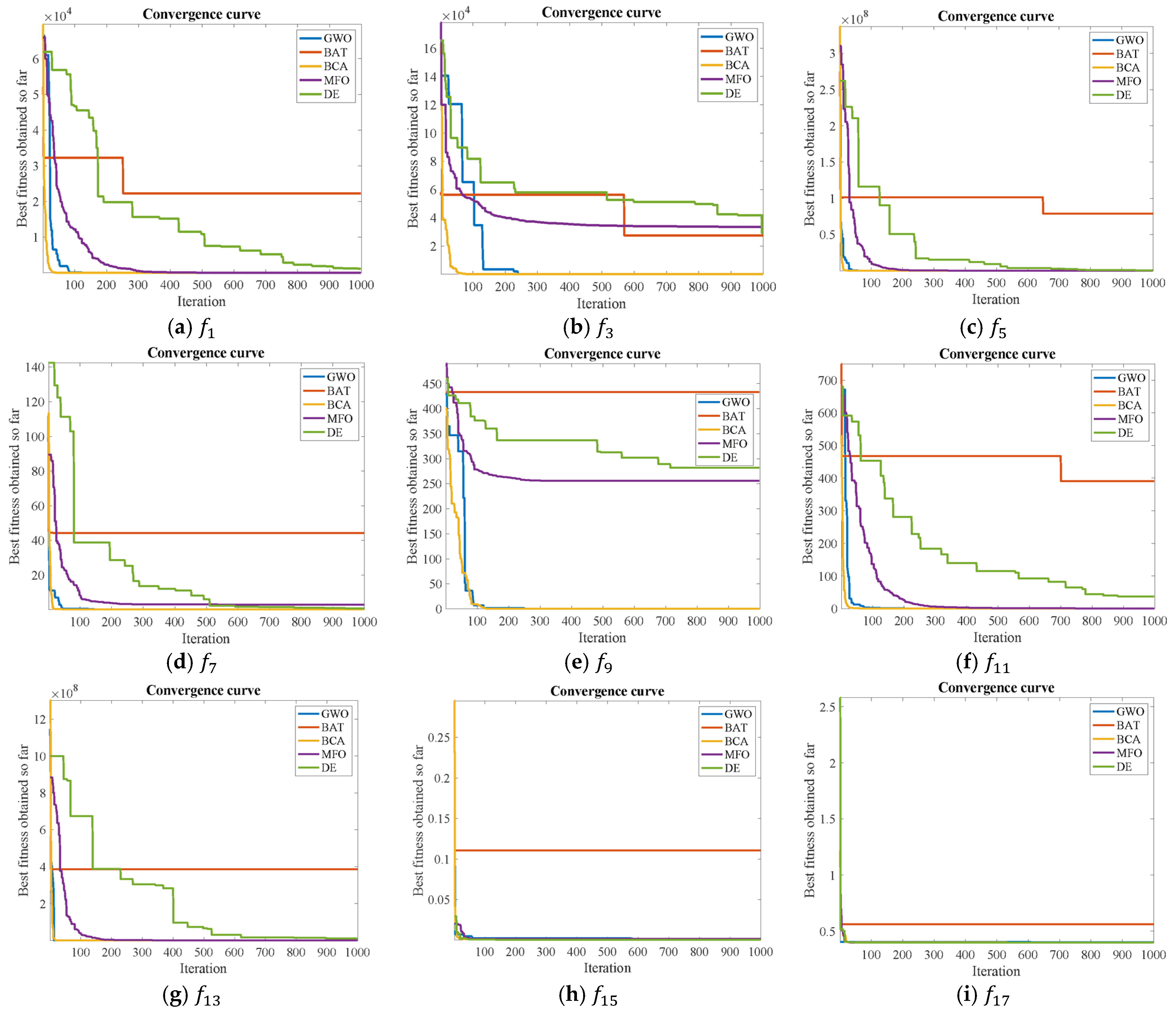
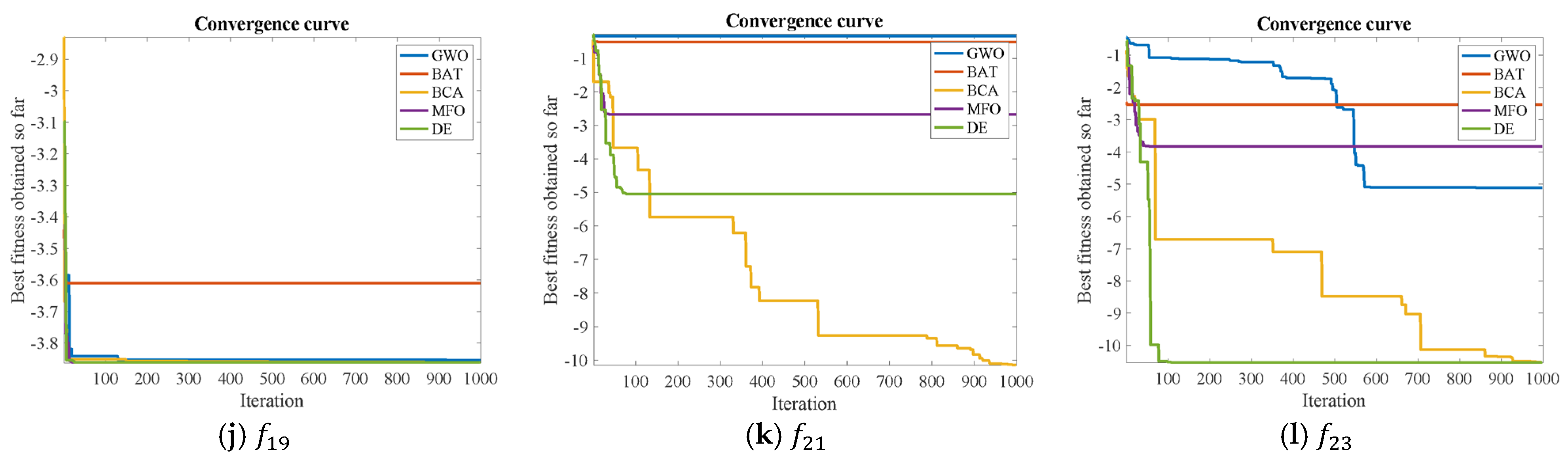
An efficient optimization algorithm should strike a good balance between intensification and diversification to overcome the exploration/exploitation dilemma. It should not converge prematurely and exhibit avoidance from local optima. To understand the convergence behavior, the convergence curves of BCA for some of the benchmark functions are compared with few other meta-heuristic approaches (DE, BAT, MFO and GWO) and shown in Figure 8. The curves represent the plot of the fitness value of the objective function versus the number of iterations. The plots reveal that BCA is very competitive and exhibits good convergence behavior as compared with other state-of-the-art optimizers for the benchmark functions.

Moreover, as it can be observed in Figure 8, the BCA demonstrates three different convergence behaviors towards function optimization. Firstly, it is observed that the convergence speeds up with the increasing number of iterations for $f_1,f_3$ and $f_9$. Secondly, we observe rapid convergence from the early stages of iterations as can be seen for unimodal functions. The convergence curves of the unimodal benchmark functions No bol($f_1,f_3,f_5, f_7$) demonstrate that BCA exploits the favorable areas of the solution space quickly and easily. Another observation is the quick avoidance of the local optima for multimodal benchmark functions $(f_9,f_{11},f_{13})$. Figure 8 also shows that the convergence to the global optima is achieved in early iterations for fixed-dimensional multimodal functions $(f_{15},f_{17},f_{19})$. For these test cases, BCA exhibits its capability of extensive diversification in fewer iterations. In addition, quick convergence is observed due to sufficient intensification of the promising areas in the search space. This behavior is witnessed due to different position-updating mechanisms and linear reduction in the propagation factor $(P_f)$ over the course of iterations. The third behavior is convergence towards the global optima only in the final iterations, as evident from the curves of the fixed-dimensional multimodal test functions $f_{21}$ and $f_{23}$. This behavior is most likely because BCA is unable to find a good solution in the early iterations, and hence it continues to search for good solutions in the problem topography to achieve convergence at global optimum.

The convergence at the global optima can also be verified by observing the search history (Figure 6) and the trajectories (Figure 7) of the thrombocytes. In Figure 6, the dense (crowded) region in the contour plots of the benchmark functions indicate that the thrombocytes converge in that region. Moreover, it is evident that BCA does not converge prematurely as the optimal solution resides in that dense region. The convergence at the global optima is also substantiated by the trajectories of the thrombocytes (Figure 7) which terminate in the region where the global optima is situated. Therefore, these plots validate that BCA is equipped with a fair balance of intensification and diversification, which helps in achieving the global optimal solution. On the whole, we can conclude that BCA has a high success rate in dealing with optimization problems.

4.3. Statistical Significance Analysis

Several non-parametric statistical tests are available in the literature for evaluating the statistical significance of the comparative results of algorithms [52]. In this paper, we utilize the well-known and frequently used Wilcoxon rank-sum test for statistical evaluation of the strength of BCA. The test is performed at a significance level of 0.05, for inspecting the significant differences between the results of BCA and other optimizers. The results (p-values) of the pair-wise comparison of BCA and other approaches are tabulated in

Table A1. p-Values of the Wilcoxon rank-sum test with 5% significance for BCA versus other algorithms for the benchmark functions with 30 independent runs. (p-values ≥ 0.05 are indicated in bold face. NaN indicates “Not a Number” reported by the test).

F	DE	PSO	GA	CS	GWO	MFO	FPA	FA	BAT	GSA	AOA	BBO
$f_1$	$3.52\times {10}^{-11}$	$2.73\times {10}^{-11}$	$3.62\times {10}^{-11}$	$3.53\times {10}^{-11}$	$3.49\times {10}^{-11}$	$3.29 \times {10}^{-11}$	$2.78\times {10}^{-11}$	$3.28\times {10}^{-11}$	$2.06\times {10}^{-11}$	$3.19\times {10}^{-11}$	$3.45\times {10}^{-11}$	$2.87\times {10}^{-11}$
$f_2$	$2.78\times {10}^{-11}$	$2.67\times {10}^{-11}$	$4.31\times {10}^{-11}$	$2.71\times {10}^{-11}$	$2.91\times {10}^{-11}$	$2.48\times {10}^{-11}$	$3.89\times {10}^{-11}$	$2.91\times {10}^{-11}$	$2.49\times {10}^{-11}$	$2.48\times {10}^{-11}$	$2.28\times {10}^{-11}$	$4.45\times {10}^{-11}$
$f_3$	$4.31\times {10}^{-11}$	$2.91\times {10}^{-11}$	$3.18\times {10}^{-11}$	$4.37\times {10}^{-11}$	$4.65\times {10}^{-11}$	$4.81\times {10}^{-11}$	$2.98\times {10}^{-11}$	$3.27\times {10}^{-11}$	$3.21\times {10}^{-11}$	$3.46\times {10}^{-11}$	$4.01\times {10}^{-11}$	$2.78\times {10}^{-11}$
$f_4$	$2.38\times {10}^{-11}$	$2.65\times {10}^{-11}$	$1.27\times {10}^{-11}$	$2.32\times {10}^{-11}$	$2.42\times {10}^{-11}$	$2.20\times {10}^{-11}$	$1.91\times {10}^{-11}$	$1.99\times {10}^{-11}$	$1.94\times {10}^{-11}$	$2.29\times {10}^{-11}$	$2.84\times {10}^{-11}$	$2.56\times {10}^{-11}$
$f_5$	$2.71\times {10}^{-11}$	$2.71\times {10}^{-11}$	$2.89\times {10}^{-11}$	$2.79\times {10}^{-11}$	$2.68\times {10}^{-11}$	$2.09\times {10}^{-11}$	$3.02\times {10}^{-11}$	$3.00\times {10}^{-11}$	$2.39\times {10}^{-11}$	$2.16\times {10}^{-11}$	$2.36\times {10}^{-11}$	$2.98\times {10}^{-11}$
$f_6$	$4.27\times {10}^{-11}$	$2.84\times {10}^{-11}$	$2.63\times {10}^{-11}$	$4.20\times {10}^{-11}$	$4.30\times {10}^{-11}$	$4.71\times {10}^{-11}$	$2.03\times {10}^{-11}$	$3.67\times {10}^{-11}$	$3.61\times {10}^{-11}$	$3.28\times {10}^{-11}$	$4.39\times {10}^{-11}$	$5.91\times {10}^{-11}$
$f_7$	$2.33\times {10}^{-11}$	$2.42\times {10}^{-11}$	$2.63\times {10}^{-11}$	$2.36\times {10}^{-11}$	$2.29\times {10}^{-11}$	$2.67\times {10}^{-11}$	$1.07\times {10}^{-11}$	$3.01\times {10}^{-11}$	$5.28\times {10}^{-11}$	$2.87\times {10}^{-11}$	$2.93\times {10}^{-11}$	$2.77\times {10}^{-11}$
$f_8$	$2.90\times {10}^{-10}$	$2.79\times {10}^{-11}$	$2.48\times {10}^{-10}$	$2.99\times {10}^{-10}$	$2.85\times {10}^{-10}$	$2.82\times {10}^{-10}$	$2.22\times {10}^{-11}$	$2.76\times {10}^{-10}$	$2.90\times {10}^{-10}$	$2.39\times {10}^{-10}$	$2.96\times {10}^{-10}$	$2.91\times {10}^{-10}$
$f_9$	$3.16\times {10}^{-12}$	$2.45\times {10}^{-11}$	$1.66\times {10}^{-12}$	$3.11\times {10}^{-12}$	$3.41\times {10}^{-12}$	$3.56\times {10}^{-12}$	$3.00\times {10}^{-11}$	$3.91\times {10}^{-12}$	$2.50\times {10}^{-12}$	$3.71\times {10}^{-12}$	$3.55\times {10}^{-12}$	$3.97\times {10}^{-12}$
$f_{10}$	$2.87\times {10}^{-12}$	$1.19\times {10}^{-12}$	$1.66\times {10}^{-12}$	$2.86\times {10}^{-12}$	$2.84\times {10}^{-12}$	$2.49\times {10}^{-12}$	$2.37\times {10}^{-11}$	$2.45\times {10}^{-12}$	$1.79\times {10}^{-12}$	$2.05\times {10}^{-12}$	$2.13\times {10}^{-12}$	$4.67\times {10}^{-12}$
$f_{11}$	$3.01\times {10}^{-11}$	$1.56\times {10}^{-13}$	$1.31\times {10}^{-12}$	$3.05\times {10}^{-11}$	$3.60\times {10}^{-11}$	$3.91\times {10}^{-11}$	$3.61\times {10}^{-11}$	$3.11\times {10}^{-11}$	$2.00\times {10}^{-11}$	$2.78\times {10}^{-11}$	$3.06\times {10}^{-11}$	$2.14\times {10}^{-11}$
$f_{12}$	$2.81\times {10}^{-11}$	$1.87\times {10}^{-11}$	$2.18\times {10}^{-11}$	$2.05\times {10}^{-11}$	$2.87\times {10}^{-11}$	$2.48\times {10}^{-11}$	$1.76\times {10}^{-11}$	$2.92\times {10}^{-11}$	$1.99\times {10}^{-11}$	$2.47\times {10}^{-11}$	$3.05\times {10}^{-11}$	$2.66\times {10}^{-11}$
$f_{13}$	$2.28\times {10}^{-11}$	$2.54\times {10}^{-11}$	$2.18\times {10}^{-11}$	$2.82\times {10}^{-11}$	$2.61\times {10}^{-11}$	$2.29\times {10}^{-11}$	$1.55\times {10}^{-11}$	$1.08\times {10}^{-11}$	$3.07\times {10}^{-11}$	$2.81\times {10}^{-11}$	$2.10\times {10}^{-11}$	$2.41\times {10}^{-11}$
$f_{14}$	$2.39\times {10}^{-9}$	$5.21\times {10}^{-8}$	$\mathbf{6.32}\mathbf{\times }{\mathbf{10}}^{\mathbf{-}\mathbf{2}}$	$6.16\times {10}^{-14}$	$7.27\times {10}^{-8}$	$3.24\times {10}^{-8}$	$\mathbf{1.81}\mathbf{\times }{\mathbf{10}}^{\mathbf{-}\mathbf{1}}$	$1.48\times {10}^{-9}$	$1.37\times {10}^{-12}$	$9.23\times {10}^{-5}$	$1.63\times {10}^{-6}$	$3.25\times {10}^{-6}$
$f_{15}$	$1.92\times {10}^{-11}$	$7.39\times {10}^{-11}$	$9.67\times {10}^{-11}$	$3.34\times {10}^{-11}$	$8.69\times {10}^{-11}$	$5.29\times {10}^{-11}$	$2.78\times {10}^{-11}$	$3.92\times {10}^{-10}$	$2.56\times {10}^{-11}$	$1.37\times {10}^{-11}$	$1.67\times {10}^{-8}$	$2.82\times {10}^{-9}$
$f_{16}$	NaN	$1.93\times {10}^{-13}$	$2.35\times {10}^{-12}$	NaN	NaN	NaN	NaN	NaN	$4.61\times {10}^{-10}$	NaN	$3.92\times {10}^{-10}$	$2.66\times {10}^{-12}$
$f_{17}$	$\mathbf{1.27}\mathbf{\times }{\mathbf{10}}^{\mathbf{-}\mathbf{1}}$	$1.84\times {10}^{-12}$	$3.28\times {10}^{-11}$	$\mathbf{1.27}\mathbf{\times }{\mathbf{10}}^{\mathbf{-}\mathbf{1}}$	$\mathbf{1.27}\mathbf{\times }{\mathbf{10}}^{\mathbf{-}\mathbf{1}}$	$\mathbf{1.27}\mathbf{\times }{\mathbf{10}}^{\mathbf{-}\mathbf{1}}$	$\mathbf{1.27}\mathbf{\times }{\mathbf{10}}^{\mathbf{-}\mathbf{1}}$	$\mathbf{1.27}\mathbf{\times }{\mathbf{10}}^{\mathbf{-}\mathbf{1}}$	$\mathbf{1.27}\mathbf{\times }{\mathbf{10}}^{\mathbf{-}\mathbf{1}}$	$2.71\times {10}^{-12}$	$1.39\times {10}^{-12}$	$1.55\times {10}^{-11}$
$f_{18}$	$8.29\times {10}^{-11}$	$2.59\times {10}^{-13}$	$4.36\times {10}^{-10}$	$3.28\times {10}^{-18}$	$2.16\times {10}^{-11}$	$1.99\times {10}^{-10}$	$3.29\times {10}^{-12}$	$1.09\times {10}^{-10}$	$2.27\times {10}^{-12}$	$6.82\times {10}^{-13}$	$3.05\times {10}^{-9}$	$3.84\times {10}^{-10}$
$f_{19}$	$3.05\times {10}^{-11}$	$2.48\times {10}^{-10}$	$2.39\times {10}^{-9}$	$2.29\times {10}^{-11}$	$2.76\times {10}^{-10}$	$1.66\times {10}^{-12}$	$8.69\times {10}^{-11}$	$3.01\times {10}^{-11}$	$2.48\times {10}^{-10}$	$5.48\times {10}^{-9}$	$3.64\times {10}^{-11}$	$3.52\times {10}^{-11}$
$f_{20}$	$3.42\times {10}^{-4}$	$7.21\times {10}^{-5}$	$3.93\times {10}^{-5}$	NaN	$4.39\times {10}^{-5}$	$2.16\times {10}^{-4}$	$1.07\times {10}^{-15}$	$8.27\times {10}^{-14}$	$2.29\times {10}^{-5}$	$1.01\times {10}^{-4}$	$2.49\times {10}^{-5}$	$3.27\times {10}^{-4}$
$f_{21}$	$1.64\times {10}^{-7}$	$8.11\times {10}^{-6}$	$3.46\times {10}^{-11}$	$7.37\times {10}^{-10}$	$1.07\times {10}^{-8}$	$1.44\times {10}^{-5}$	$5.28\times {10}^{-10}$	$1.05\times {10}^{-12}$	$2.45\times {10}^{-8}$	$2.91\times {10}^{-8}$	$1.38\times {10}^{-8}$	$2.16\times {10}^{-9}$
$f_{22}$	$1.34\times {10}^{-11}$	$6.47\times {10}^{-11}$	$1.98\times {10}^{-11}$	$5.71\times {10}^{-11}$	$5.37\times {10}^{-11}$	$3.59\times {10}^{-11}$	$2.46\times {10}^{-11}$	$2.04\times {10}^{-10}$	$2.38\times {10}^{-11}$	$4.28\times {10}^{-12}$	$1.09\times {10}^{-8}$	$1.89\times {10}^{-9}$
$f_{23}$	NaN	$1.28\times {10}^{-12}$	$2.05\times {10}^{-10}$	$2.51\times {10}^{-11}$	$1.94\times {10}^{-8}$	$4.85\times {10}^{-9}$	$8.37\times {10}^{-8}$	$1.39\times {10}^{-9}$	$4.37\times {10}^{-12}$	$3.61\times {10}^{-8}$	$2.57\times {10}^{-10}$	$3.08\times {10}^{-8}$

(see Appendix A). The p-values < 0.05 reveal the superiority of BCA. With regard to the obtained p-values in Table A1, we observe that the proposed BCA significantly outperforms its competitors. Statistically meaningful differences in the results are witnessed for the majority of the test cases.

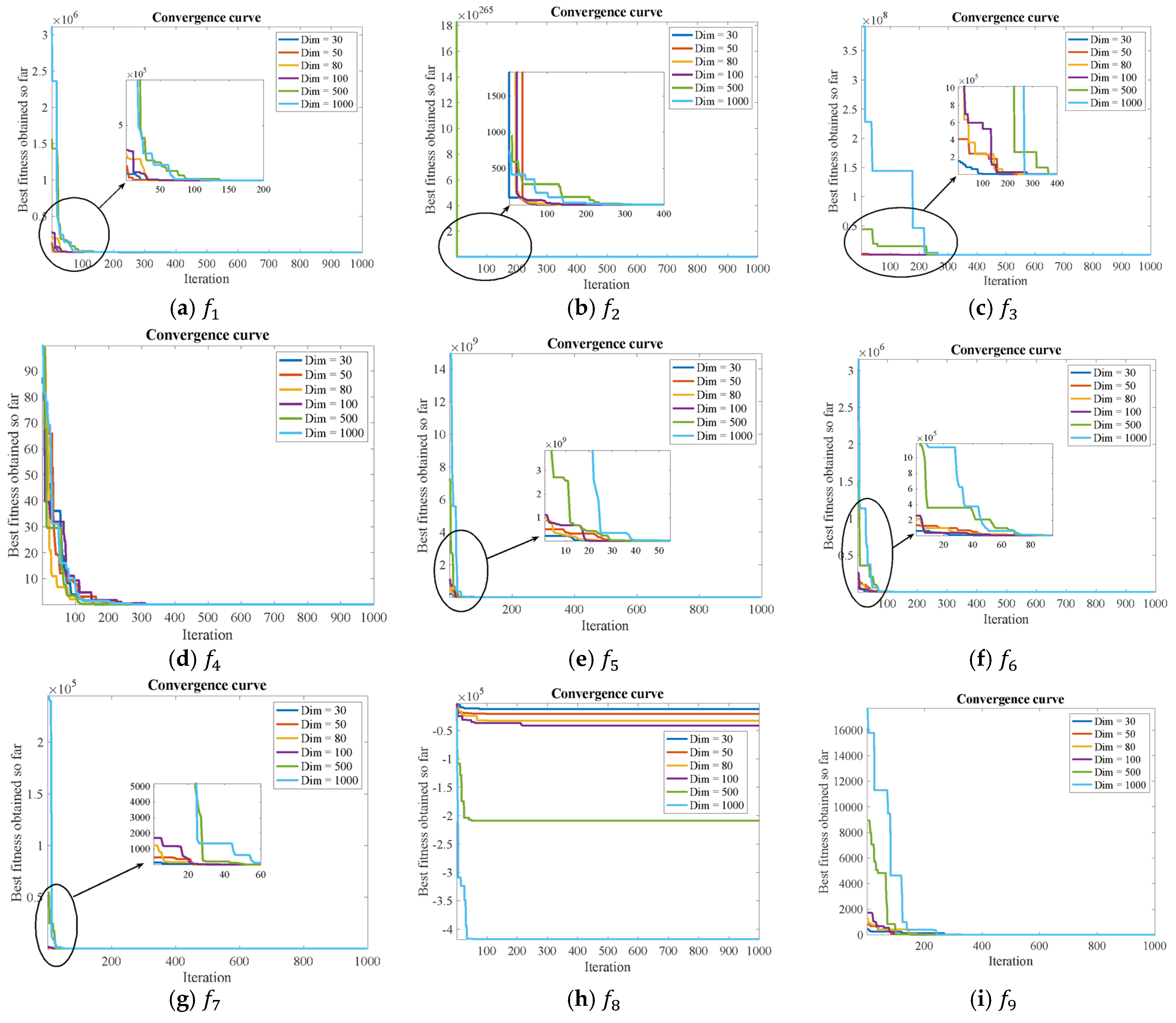
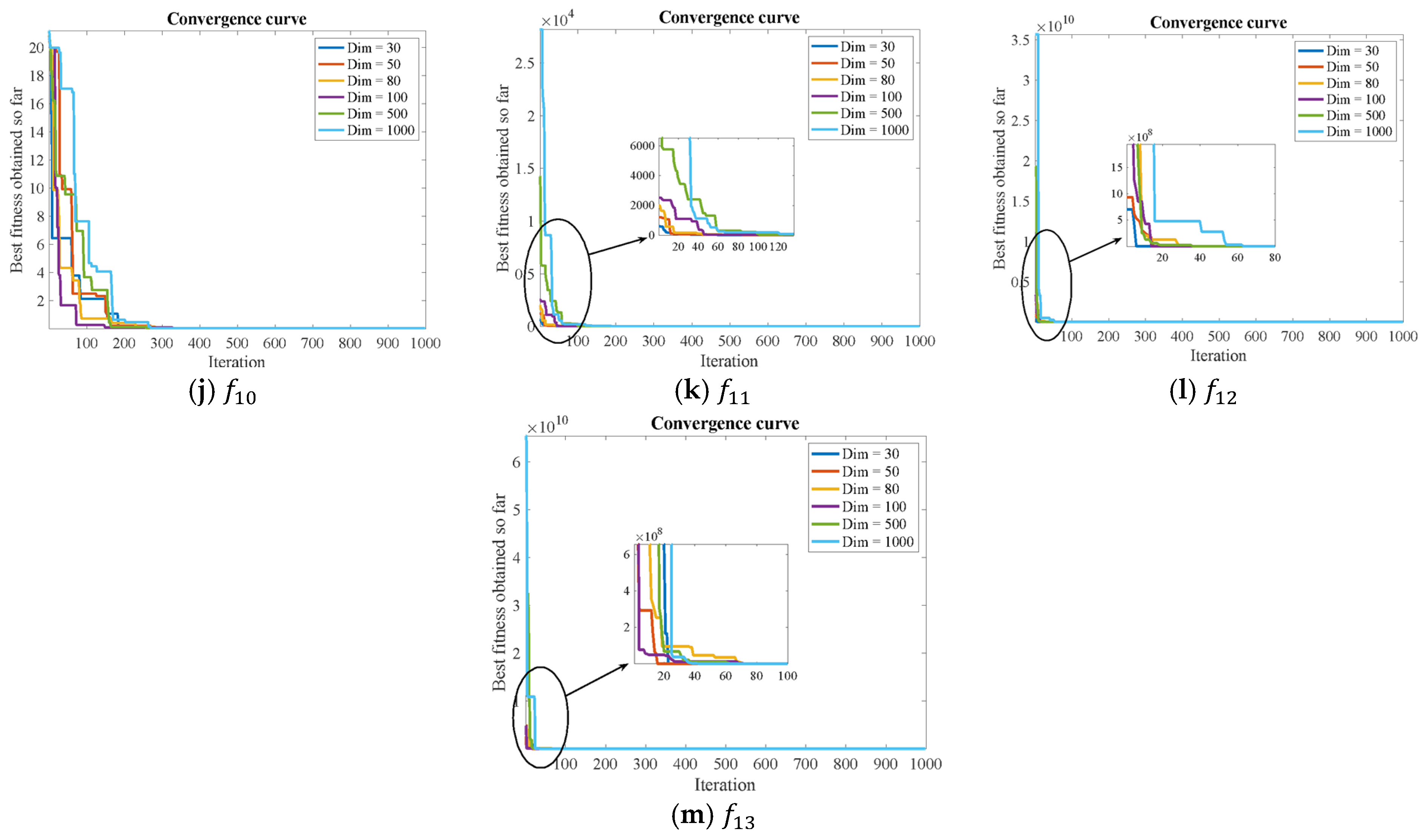
4.4. Influence of High Dimensionality

In this subsection, we utilize a scalability assessment to demonstrate the efficient performance of BCA in dealing with high dimensional problems. The scalability analysis reveals the influence of dimensionality on the solution quality and helps in identifying the efficacy of the optimizer for not only low-dimensional problems but also for problems with large dimensions. In this paper, we evaluate the efficiency of BCA by utilizing it to tackle both unimodal $(f_1-f_7)$ and multimodal $(f_8-f_{13})$ problems with different dimensions. All these scalable benchmark functions are solved with 30, 50, 80, 100, 500 and 1000 dimensions. Figure 9 illustrates the scalability results (performance) of BCA for various test functions on different dimensionality. Referring to Figure 9, the convergence curves reveal that the proposed BCA exhibits good performance and validates its applicability on high dimensional environments as well. It is observed that BCA is capable of finding the optimal solutions in early iterations. As per the curves in Figure 9, BCA upholds a good balance between the intensification and diversification tendencies on multivariable optimization problems. Moreover, we record the mean and SD of the acquired results over 1000 iterations and 30 runs of BCA for 30, 100 and 1000 dimensions. The acquired results in dealing with $f_1-f_{13}$ test cases with different dimensions are reported in

Table 6. Influence of high dimensionality on the performance of BCA: Results of benchmark functions ($f_1-f_{13}$) with different dimensions.

Benchmark	Dimensions = 30		Dimensions = 100		Dimensions = 1000
	Mean	SD	Mean	SD	Mean	SD
$f_1$	9.80 $\times {10}^{-28}$	1.70 $\times {10}^{-22}$	5.06 $\times {10}^{-15}$	1.95 $\times {10}^{-14}$	1.24 $\times {10}^{-13}$	3.93 $\times {10}^{-13}$
$f_2$	8.91 $\times {10}^{-17}$	1.36 $\times {10}^{-11}$	9.80 $\times {10}^{-8}$	5.24 $\times {10}^{-7}$	2.60 $\times {10}^{-7}$	8.97 $\times {10}^{-7}$
$f_3$	7.63 $\times {10}^{-16}$	2.46 $\times {10}^{-15}$	2.40 $\times {10}^{-11}$	9.48 $\times {10}^{-11}$	1.35 $\times {10}^{-8}$	5.71 $\times {10}^{-8}$
$f_4$	7.01 $\times {10}^{-10}$	1.77 $\times {10}^{-9}$	1.95 $\times {10}^{-8}$	8.32 $\times {10}^{-8}$	5.08 $\times {10}^{-8}$	1.52 $\times {10}^{-7}$
$f_5$	3.72	8.72	3.34 $\times {10}^1$	3.69 $\times {10}^1$	5.41 $\times {10}^1$	3.85 $\times {10}^1$
$f_6$	1.36 $\times {10}^{-2}$	9.83 $\times {10}^{-3}$	3.25 $\times {10}^{-1}$	2.59 $\times {10}^{-1}$	7.73 $\times {10}^1$	4.58 $\times {10}^1$
$f_7$	3.95 $\times {10}^{-4}$	4.78 $\times {10}^{-4}$	5.25 $\times {10}^{-4}$	4.79 $\times {10}^{-4}$	6.34 $\times {10}^{-4}$	7.71 $\times {10}^{-4}$
$f_8$	−1.25 $\times {10}^4$	4.30 $\times {10}^1$	−4.18 $\times {10}^4$	2.01 $\times {10}^2$	−4.18 $\times {10}^5$	4.36 $\times {10}^3$
$f_9$	1.70 $\times {10}^{-14}$	3.04 $\times {10}^{-14}$	4.92 $\times {10}^{-14}$	1.06 $\times {10}^{-13}$	1.81 $\times {10}^{-12}$	2.70 $\times {10}^{-12}$
$f_{10}$	8.88 $\times {10}^{-16}$	2.89 $\times {10}^{-11}$	7.27 $\times {10}^{-10}$	2.34 $\times {10}^{-9}$	9.14 $\times {10}^{-9}$	2.78 $\times {10}^{-8}$
$f_{11}$	3.49 $\times {10}^{-15}$	1.86 $\times {10}^{-14}$	2.16 × 10−15	7.31 $\times {10}^{-15}$	5.55 $\times {10}^{-15}$	2.60 $\times {10}^{-14}$
$f_{12}$	4.19 $\times {10}^{-6}$	5.43 $\times {10}^{-4}$	2.31 $\times {10}^{-3}$	1.28 $\times {10}^{-3}$	2.74 $\times {10}^{-3}$	1.64 $\times {10}^{-3}$
$f_{13}$	1.99 $\times {10}^{-3}$	5.37 $\times {10}^{-3}$	7.14 $\times {10}^{-2}$	5.95 $\times {10}^{-2}$	1.01	7.95 $\times {10}^{-1}$

. As can be seen in Table 6, the proposed BCA demonstrates consistent performance when dealing with many variables for the majority of the test functions. In a nutshell, the experimental results show the scalability of the proposed BCA and prove its efficiency for high-dimensional tasks.

5. BCA for Standard Engineering Problems

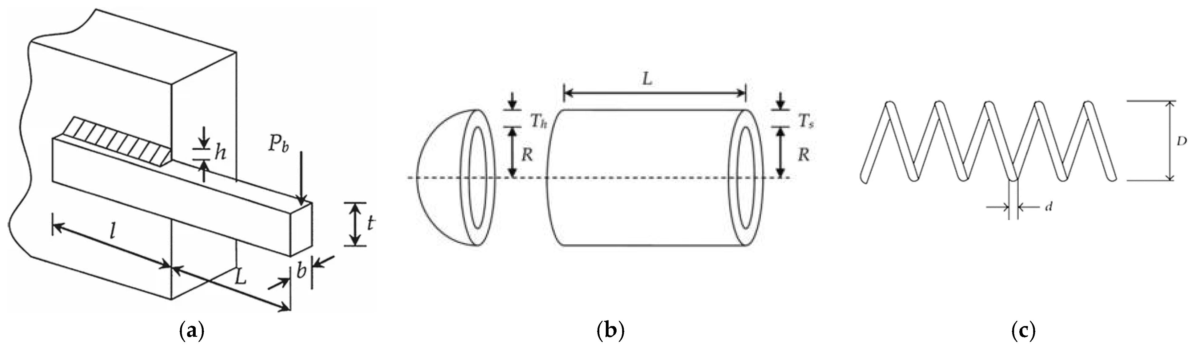
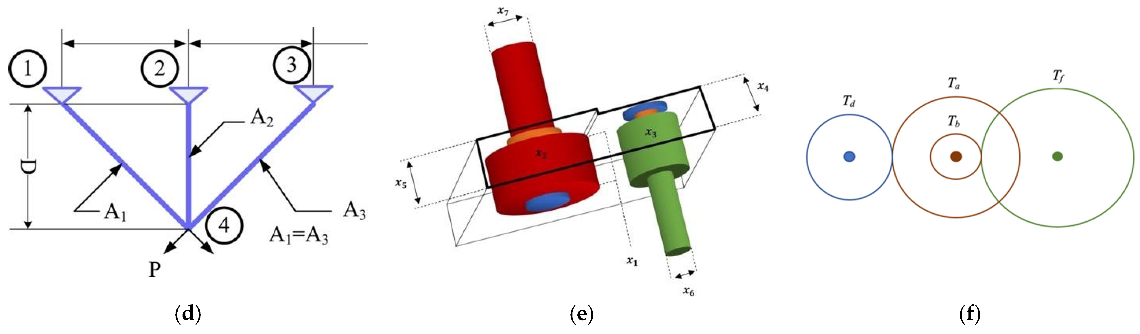
In this section, the proficiency and capability of the proposed algorithm (BCA) in addressing real-world engineering optimization (constrained and unconstrained) problems is demonstrated by employing it on standard engineering design tasks. The BCA is utilized to solve six well-known benchmark engineering design problems: welded beam design problem, pressure vessel design problem, tension/compression spring design problem, three-bar truss design problem, speed reducer design problem and gear train design problem. Figure 10 illustrates the schematic views of these design problems.

Table 7. Brief description of the tackled engineering design optimization problems.

No.	Problem	Dim	Constr	Objective	Description of variables
1	Welded beam design	4	7	Minimize cost	$\mathrm{thickness} \mathrm{of} \mathrm{weld} (h$) $\mathrm{length} \mathrm{of} \mathrm{the} \mathrm{clamped} \mathrm{bar} (l$) $\mathrm{height} \mathrm{of} \mathrm{the} \mathrm{bar} (t$) $\mathrm{thickness} \mathrm{of} \mathrm{the} \mathrm{bar} (b$)
2	Pressure vessel design	4	4	Minimize cost	$\mathrm{the} \mathrm{thickness} \mathrm{of} \mathrm{the} \mathrm{shell} (T_s$) $\mathrm{the} \mathrm{thickness} \mathrm{of} \mathrm{the} \mathrm{head} (T_h$) $\mathrm{the} \mathrm{inner} \mathrm{radius} (R$) $\mathrm{the} \mathrm{length} \mathrm{of} \mathrm{the} \mathrm{cylindrical} \mathrm{section} \mathrm{without} \mathrm{considering} \mathrm{the} \mathrm{head} (L$)
3	Tension/compression spring design	3	4	Minimize weight	$\mathrm{wire} \mathrm{diameter} (d$) $\mathrm{mean} \mathrm{coil} \mathrm{diameter} (D$) $\mathrm{number} \mathrm{of} \mathrm{active} \mathrm{coils} (N$)
4	Three-bar truss design	2	3	Minimize weight	$\mathrm{area} \mathrm{of} \mathrm{bars} 1 \mathrm{and} 3 (A_1$) $\mathrm{area} \mathrm{of} \mathrm{bar} 2 (A_2$)
5	Speed reducer design	7	11	Minimize weight	$\mathrm{Face} \mathrm{width} (x_1$) $\mathrm{Teeth} \mathrm{module} (x_2$) $\mathrm{Number} \mathrm{of} \mathrm{teeth} (x_3$) $\mathrm{First} \mathrm{shaft} \mathrm{length} (x_4$) $\mathrm{Sec}\mathrm{ond} \mathrm{shaft} \mathrm{length} (x_5$) $\mathrm{First} \mathrm{shaft} \mathrm{diameter} (x_6$) $\mathrm{Sec}\mathrm{ond} \mathrm{shaft} \mathrm{diameter} (x_7$)
6	Gear train design	4	0	Minimize gear ratio	$\mathrm{Gear} \mathrm{teeth}\text{:} T_a, T_b, T_d, T_f$

Note: Dim = number of variables, Constr = total number of constraints.

presents an overview of the undertaken engineering design optimization tasks and the variables involved in these problems. To solve these problems, the BCA is applied based on 30 independent runs with the population size $\left(N_{Pop}\right)$ of 30 and 1000 iterations in each run. The results of BCA are compared with other state-of-the-art powerful meta-heuristic approaches in the literature. Since the engineering design problems have various constraints, we need to incorporate a constraint handling method with the BCA. For the sake of simplicity, we utilize the death penalty (scalar penalty function) as the method for handling the constraints [53]. In this constraint handling technique, solutions which violate any of the constraints are penalized by a large fitness value (in case of minimization).

5.1. Welded Beam Design Problem

The welded beam design problem is one of the classical benchmark problems whose objective is to minimize the fabrication cost of the welded beam. The schematic of the welded beam structure is shown in Figure 10a. This design problem is subject to constraints on shear stress ($\tau$) and bending stress in the beam ($\sigma$), buckling load ($P_c$), end deflection of the beam ($\delta$). The design variables are tabulated in Table 7. The optimization task for this design problem can be mathematically formulated as follows:

Consider	$x=\left[x_1 x_2 x_3 x_4\right]=\left[h l t b\right]$
Minimize	$f\left(x\right)=1.10471x_1^2{x}_2+0.04811x_3{x}_4\left(14.0+x_2\right)$
Subject to	$g_1\left(x\right)=\tau \left(x\right)-{\tau }_{max}\le 0$ $g_2\left(x\right)=\sigma \left(x\right)-{\sigma }_{max}\le 0,$ $g_3\left(x\right)=\delta \left(x\right)-{\delta }_{max}\le 0,$ $g_4\left(x\right)=x_1-x_4\le 0,$ $g_5\left(x\right)=P-P_c\left(x\right)\le 0,$ $g_6\left(x\right)=0.125-x_1\le 0,$ $g_7\left(x\right)=1.10471x_1^2+0.04811x_3{x}_4\left(14.0+x_2\right)-5.0\le 0,$
Variable range	$0.1\le x_1\le 2,$ $0.1\le x_2\le 10,$ $0.1\le x_3\le 10,$ $0.1\le x_4\le 2$
where	$\tau \left(x\right)=\sqrt{{\left({\tau }^{\prime }\right)}^2+2{\tau }^{\prime }{\tau }^{″}\frac{x_2}{2R}+{\left({\tau }^{″}\right)}^2}$, ${\tau }^{\prime }=\frac{P}{\sqrt{2}{x}_1{x}_2}, {\tau }^{″}=\frac{MR}{J}, M=P\left(L+\frac{x_2}{2}\right),$ $R=\sqrt{\frac{x_2^2}{4}+{\left(\frac{x_1+x_3}{2}\right)}^2},$ $J=2\left\{\sqrt{2}{x}_1{x}_2\left[\frac{x_2^2}{4}+{\left(\frac{x_1+x_3}{2}\right)}^2\right]\right\},$ $\sigma \left(x\right)=\frac{6PL}{x_4{x}_3^2} , \delta \left(x\right)=\frac{6P{L}^3}{E{x}_4{x}_3^2}$ $P_c\left(x\right)=\frac{4.013E\sqrt{\frac{x_3^2{x}_4^6}{36}}}{L^2}\left(1-\frac{x_3}{2L}\sqrt{\frac{E}{4G}}\right),$ $P=6000 lb, L=14 in., {\delta }_{max}=0.25 in.,$ $E=30\times {10}^6 psi, G=12\times {10}^6 psi,$ ${\tau }_{max}=13,600 psi, {\sigma }_{max}=30,000 psi$

This engineering design optimization problem has been addressed by many researchers using a number of algorithms. The comparative results of the best solution obtained by BCA and other algorithms are presented in

Table 8. Comparison of the best solution obtained by BCA with other algorithms in the literature for the welded beam design problem.

Algorithm	Optimal Values of Design Variables				Optimal Cost
	$\mathit{h}$	$\mathit{l}$	$\mathit{t}$	$\mathit{b}$
BCA	0.205729	3.470471	9.036622	0.205729	1.72484
HHO [12]	0.204039	3.531061	9.027463	0.206147	1.73199057
RANDOM [54]	0.4575	4.7313	5.0853	0.66	4.1185
DAVID [54]	0.2434	6.2552	8.2915	0.2444	2.3841
SIMPLEX [54]	0.2792	5.6256	7.7512	0.2796	2.5307
APPROX [54]	0.2444	6.2189	8.2915	0.2444	2.3815
GA [55]	0.248900	6.173000	8.178900	0.253300	2.433116
GA [56]	0.208800	3.420500	8.997500	0.210000	1.748310
HS [57]	0.2442	6.2231	8.2915	0.2443	2.3807
ESs [58]	0.199742	3.61206	9.0375	0.206082	1.7373
CDE [59]	0.203137	3.542998	9.033498	0.206179	1.733462
MFO [14]	0.203567	3.443025	9.230278	0.212359	1.732541
MVO [60]	0.205611	3.472103	9.040931	0.205709	1.725472
SCA [25]	0.204695	3.536291	9.004290	0.210025	1.759173
GA [49]	0.164171	4.032541	10.00000	0.223647	1.873971
ES [61]	0.199742	3.612060	9.037500	0.20682	1.73730
SA [62]	0.20564426	3.472578742	9.03662391	0.2057296	1.7250022
Co-evolutionary PSO [63]	0.20573	3.47049	9.03662	0.20573	1.72485084
GSA [23]	0.18219	3.856979	10.0000	0.202376	1.879952
Improved PSO [64]	0.205729	3.470488	9.036624	0.205729	1.724852
DE [65]	0.20573	3.470489	9.0336624	0.205730	1.724852
CS [13]	0.2015	3.562	9.0414	0.2057	1.73121
ABC [66]	0.205730	3.470489	9.036624	0.205730	1.724852
ACO [67]	0.205700	3.471131	9.036683	0.205731	1.724918
PO [47]	0.205730	3.470472	9.036624	0.205730	1.724851
CAEP [68]	0.205700	3.470500	9.036600	0.205700	1.724852
HGA [69]	0.205700	3.470500	9.036600	0.205700	1.7249
WCA [27]	0.205728	3.470522	9.036620	0.205729	1.724856
CGWO [70]	0.343891	1.883570	9.031330	0.212121	1.725450
GWO [9]	0.205676	3.478377	9.036810	0.205778	1.726240
CPSO [71]	0.202369	3.544214	9.048210	0.205723	1.728024
GA [72]	0.205986	3.471328	9.020224	0.206480	1.728226
WOA [10]	0.205396	3.484293	9.037426	0.206276	1.730499
CS [73]	0.182200	3.795100	9.998100	0.211100	1.946000
BA [74]	0.154300	5.736100	8.862700	0.229700	2.084000
CapSA [75]	0.205723	3.470789	9.036622	0.205737	1.7249

. From the results in Table 8, it is evident that the proposed BCA yields an optimal design with minimum cost and outperforms all other algorithms. Moreover, the statistical results (obtained by 30 independent executions of BCA) in terms of the best value, worst value, mean value, and standard deviation are compared with existing algorithms in the literature and reported in

Table 9. Comparison of statistical results of BCA with other optimization algorithms in the literature for solving the welded beam design problem.

Algorithm	Best	Worst	Mean	SD #
BCA	1.72484	1.7272306	1.7254101	$4.237\times {10}^{-7}$
MFO [14]	1.732541	1.802364	1.775231	0.012397
MVO [60]	1.725472	1.741651	1.729680	0.004866
SCA [25]	1.759173	1.873408	1.817657	0.027543
GA [49]	1.873971	2.320125	2.119240	0.034820
ES [61]	1.728226	1.993408	1.792654	0.07471
SA [62]	1.7250022	1.8843960	1.7564428	NA
Co-evolutionary PSO [63]	1.728024	1.782143	1.748831	0.012926
Improved PSO [64]	1.724852	NA *	2.0574	0.2154
DE [65]	1.724852	1.725000	1.725	$1.0\times {10}^{-15}$
CS [13]	1.7312065	2.3455793	1.8786560	0.2677989
ABC [66]	1.724852	NA	1.741913	0.031
ACO [67]	1.72918	1.775961	1.729752	0.009200
PO [47]	1.724851	1.724852	1.724851	$2.53\times {10}^{-7}$
CAEP [68]	1.724852	3.179709	1.971809	0.443000
WCA [27]	1.724856	1.744697	1.726427	0.004290
CGWO [70]	1.725450	2.435700	2.428900	1.357800
CPSO [71]	1.728024	1.782143	1.748831	0.012900
CapSA [75]	1.72481904	1.72723071	1.72541110	$4.2376\times {10}^{-7}$
PSO-DE [76]	1.724852	1.724852	1.724852	$6.7\times {10}^{-16}$
COMDE [77]	1.724852	1.724852	1.724852	$1.6\times {10}^{-12}$
DELC [78]	1.724852	1.724852	1.724852	$4.1\times {10}^{-13}$
MADE [79]	1.724852	1.724852	1.724852	$9.6\times {10}^{-16}$
AMDE [80]	1.724852	1.724852	1.724852	$1.1\times {10}^{-15}$

* NA is Not available, ^# Standard Deviation.

. The statistical results for the welded beam design problem in Table 9 show that BCA finds the best values and exhibits better performance as compared to the other optimizers. This confirms the competence of BCA in addressing this optimization problem.

5.2. Pressure Vessel Design Problem

Another widely accepted structural design benchmark problem is the design of the pressure vessel. In this well-regarded case, the objective is to minimize the total fabrication cost (material, forming and welding) of the cylindrical pressure vessel. The vessel is capped at both the ends wherein the heads have a hemi-spherical shape. The schematic is illustrated in Figure 10b and the design variables are described in Table 7. The mathematical formulation of the optimization model for this design problem is as follows:

Consider	$x=\left[x_1 x_2 x_3 x_4]=[T_s T_h R L\right]$
Minimize	$f\left(x\right)=0.6224x_1{x}_3{x}_4+1.7781x_2{x}_3^2+3.1661x_1^2{x}_4+19.84x_1^2{x}_3$
Subject to	$g_1\left(x\right)=-x_1+0.0193x_3\le 0$ $g_2\left(x\right)=-x_2+0.00954x_3\le 0,$ $g_3\left(x\right)=-\pi x_3^2{x}_4-\frac{4}{3}\pi x_3^3+1,296,000\le 0,$ $g_4\left(x\right)=x_4-240\le 0,$
Variable range	$0\le x_1\le 99,$ $0\le x_2\le 99,$ $10\le x_3\le 200,$ $10\le x_4\le 200$

This design problem has been addressed by many researchers using different algorithms, including meta-heuristic approaches as well as mathematical techniques.

Table 10. Comparison of the best solution obtained by BCA with other algorithms in the literature for the pressure vessel design problem.

Algorithm	Optimal Values of Design Variables				Optimal Cost
	${\mathit{T}}_{\mathit{s}}$	${\mathit{T}}_{\mathit{h}}$	$\mathit{R}$	$\mathit{L}$
BCA	0.7782	0.3847	40.3215	199.973	5885.3991
MFO [14]	0.835241	0.409854	43.578621	152.21520	6055.6378
MVO [60]	0.845719	0.418564	43.816270	156.38164	6011.5148
SCA [25]	0.817577	0.417932	41.74939	183.57270	6137.3724
GA [49]	0.752362	0.399540	40.452514	198.00268	5890.3279
HS [81]	1.099523	0.906579	44.456397	179.65887	6550.0230
DA [82]	0.782825	0.384649	40.3196	200	5923.11
Co-evolutionary PSO [63]	0.812500	0.437500	42.091266	176.746500	6061.077
ES [61]	0.812500	0.437500	42.098087	176.640518	6059.7456
CS [13]	0.812500	0.437500	42.0984456	176.6363595	6059.7143348
ABC [83]	0.812500	0.437500	42.098446	176.636596	6059.714339
Improved PSO [84]	0.812500	0.437500	42.098445	176.6365950	6059.7143
Penalty guided ABC [85]	0.7781686	0.3846491	40.3210545	199.9802367	5885.40322828
DE [65]	0.812500	0.437500	42.098446	176.6360470	6059.701660
WOA [10]	0.812500	0.437500	42.0982699	176.638998	6059.7410
PO [47]	0.7782	0.3847	40.3215	199.9733	5885.3997
NMPSO [86]	0.8036	0.3972	41.6392	182.4120	5930.3137
GWO [9]	0.8125	0.4345	42.0892	176.7587	6051.5639
HPSO [87]	0.8125	0.4375	42.0984	176.6366	6059.7143
G-QPSO [88]	0.8125	0.4375	42.0984	176.6372	6059.7208
CDE [59]	0.8125	0.4375	42.0984	176.6376	6059.7340
DE [5]	0.8125	0.4375	42.0984	176.6377	6059.7340
GA [72]	0.8125	0.4375	42.0974	176.6540	6059.9463
CPSO [71]	0.8125	0.4375	42.0913	176.7465	6061.0777
GSA [23]	1.1250	0.6250	55.9887	84.4542	8538.8359
HHO [12]	0.81758383	0.4072927	42.09174576	176.7196352	6000.46259
GA [55]	0.812500	0.437500	42.097398	176.654050	6059.9463
Lagrangian multiplier (Kannan) [10]	1.125000	0.625000	58.291000	43.6900000	7198.0428
Branch-bound (Sandgren) [10]	1.125000	0.625000	47.700000	117.701000	8129.1036
DELC [78]	0.812500	0.437500	42.0984456	176.6365958	6059.7143
CSS [89]	0.812500	0.437500	42.103624	176.572656	6059.0888
ESs [58]	0.812500	0.437500	42.098087	176.640518	6059.7456

presents a comparison of the optimal solutions acquired by BCA and other eminent algorithms in the erstwhile literature for the pressure vessel design problem. Inspecting the results in Table 10, we observe that the BCA offers competitive results to PO and superior results when compared with other optimizers. Therefore, we conclude that the proposed BCA is capable of finding feasible optimal design for the pressure vessel at minimum cost (of 5885.3991). Further, the statistical results (i.e., the best, worst, mean and standard deviation values) of BCA and other optimizers for the pressure vessel design problem are presented in

Table 11. Comparison of statistical results of BCA with other optimization algorithms in the literature for solving the pressure vessel design problem.

Algorithm	Best	Worst	Mean	SD #
BCA	5885.3991	5910.5321	5891.3265	8.4237
MFO [14]	6055.6378	7023.8521	6360.6854	365.597
MVO [60]	6011.5148	7250.9170	6477.3050	327.007
SCA [25]	6137.3724	6512.3541	6326.7606	126.609
GA [49]	5890.3279	7005.7500	6264.0053	496.128
HS [81]	6550.0230	8005.4397	6643.9870	657.523
DA [82]	5923.11	222536	21342.2	47044.2
Co-evolutionary PSO [63]	6061.077	6363.8041	6147.1332	86.4545
ES [61]	6059.7456	7332.8798	6850.004	9426.000
CS [13]	6059.714	6495.3470	6447.7360	502.693
ABC [83]	6059.714339	NA *	6245.308144	205
Improved PSO [84]	6059.7143	NA	6289.92881	305.78
WOA [10]	NA	NA	6068.0500	65.6519
GSA [23]	NA	NA	8932.9500	683.5475
PO [47]	5885.3997	5908.0250	5891.8068	8.4746
NMPSO [86]	5930.3137	5960.0557	5946.7901	9.1610
PSO-DE [76]	6059.7140	NA	6059.7140	NA
HPSO [87]	6059.7143	6288.6770	6099.9323	86.2000
CPSO [71]	6061.0777	6363.8041	6147.1332	86.4500
GWO [9]	6051.5630	6395.3600	6159.3200	379.6740
G-QPSO [88]	6059.7208	7544.4925	6440.3786	448.4711

* NA is Not available, ^# Standard Deviation.

. According to the results in this table, it is shown that the performance of proposed BCA is superior and significantly better than other optimizers. BCA outperforms most of the algorithms mentioned in Table 11. We observe that the standard deviation acquired by BCA is 8.4237, which is considerably lower when compared to other algorithms. Thus, BCA proves to be reliable and efficient for solving this optimization problem.

5.3. Tension/Compression Spring Design Problem

The goal of the tension/compression spring design problem [90] is to minimize the weight of the spring shown in Figure 10c. The constraints for optimum design are based on shear stress, surge frequency and deflection. The design variables of this optimization problem are defined in Table 7. The optimization problem is mathematically represented as follows:

Consider	$x=\left[x_1 x_2 x_3\right]=\left[d D N\right]$
Minimize	$f\left(x\right)=\left(x_3+2\right)x_2{x}_1^2$
Subject to	$g_1\left(x\right)=1-\frac{x_2^2{x}_3}{71785x_1^4}\le 0$, $g_2\left(x\right)=\frac{4x_2^2-x_1{x}_2}{12566\left(x_2{x}_1^3-x_1^4\right)}+\frac{1}{5108x_1^2}\le 0,$ $g_3\left(x\right)=1-\frac{140.45x_1}{x_2^2{x}_3}\le 0,$ $g_4\left(x\right)=\frac{x_1+x_2}{1.5}-1\le 0,$
Variable range	$0.05\le x_1\le 2.00,$ $0.25\le x_2\le 1.30,$$2.00\le x_3\le 15.0$

Several optimizers have been previously applied to solve this design problem.

Table 12. Comparison of the best solution obtained by BCA with other algorithms in the literature for the tension/compression spring design problem.

Algorithm	Optimal Values of Design Variables			Optimal Cost
	$\mathit{d}$	$\mathit{D}$	$\mathit{N}$
BCA	0.05248	0.37594	10.24509	0.01267
PO [47]	0.05248	0.37594	10.24509	0.01267
DEDS [91]	0.05169	0.35672	11.28897	0.01267
HEAA [92]	0.05169	0.35673	11.28829	0.01267
DELC [78]	0.05169	0.35672	11.28897	0.01267
WCA [27]	0.05168	0.35652	11.30041	0.01267
MADE [79]	0.05169	0.35672	11.28897	0.01267
GWO [9]	0.05169	0.35674	11.28885	0.01267
DE [5]	0.05161	0.35471	11.41083	0.01267
HS [81]	0.05115	0.34987	12.07643	0.01267
CPSO [71]	0.05173	0.35764	11.24454	0.01267
WOA [10]	0.05121	0.34522	12.00403	0.01268
GA [72]	0.05199	0.36397	10.89052	0.01268
GSA [23]	0.05028	0.32368	13.52541	0.01270
MFO [14]	0.05000	0.313501	14.03279	0.012753902
MVO [60]	0.05000	0.315956	14.22623	0.012816930
SCA [25]	0.050780	0.334779	12.72269	0.012709667
SSA [17]	0.051207	0.345215	12.004032	0.0126763

presents the comparison of the optimal results achieved by BCA and other algorithms for the tension/compression spring design problem. Table 12 suggests that BCA is able to find an optimum design of the spring with the minimum weight. Further, the statistical results are compared with other approaches in the literature and reported in

Table 13. Comparison of statistical results of BCA with other optimization algorithms in the literature for solving the tension/compression spring design problem.

Algorithm	Worst	Mean	Best	SD #
BCA	0.0127	0.0127	0.0127	0.0000
PO [47]	0.0128	0.0127	0.0127	0.0000
DELC [78]	0.0127	0.0127	0.0127	0.0000
HEAA [92]	0.0127	0.0127	0.0127	0.0000
PSO–DE [76]	0.0127	0.0127	0.0127	0.0000
MADE [79]	0.0127	0.0127	0.0127	0.0000
AMDE [80]	0.0127	0.0127	0.0127	0.0000
DEDS [91]	0.0127	0.0127	0.0127	0.0000
DE [5]	0.0128	0.0127	0.0127	0.0000
HPSO [87]	0.0127	0.0127	0.0127	0.0000
ABC [83]	NA *	0.0127	0.0127	0.0128
CPSO [71]	0.0129	0.0127	0.0127	0.0005
GA [72]	0.0130	0.0127	0.0127	0.0001
WCA [27]	0.0130	0.0127	0.0127	0.0001
G-QPSO [88]	0.0178	0.0135	0.0127	0.0013
CAEP [68]	0.0151	0.0136	0.0127	0.0008
GSA [23]	NA	0.0136	NA	0.0026

* NA is Not available, ^# Standard Deviation.

. It can be seen that BCA either outperforms or performs equivalently to all other algorithms listed in Table 13.

5.4. Three-Bar Truss Design Problem

This engineering design problem is one of the well-regarded optimization problems and frequently addressed since it has a very restricted search space. The aim is to find an optimal design of a truss with three bars such that its weight is minimum. The structural design parameters of this problem are shown in Figure 10d and the details are given in Table 7. There are several constraints including stress, deflection, and buckling. The mathematical representation of this problem is as follows:

Consider	$x=\left[x_1 x_2]=[A_1 A_2\right]$
Minimize	$f\left(x\right)=\left( 2\sqrt{2}{x}_1+x_2\right)l$
Subject to	$g_1\left(x\right)=\frac{ \sqrt{2}{x}_1+x_2}{\sqrt{2}{x}_1^2+2x_1{x}_2}P-\sigma \le 0$, $g_2\left(x\right)=\frac{ x_2}{\sqrt{2}{x}_1^2+2x_1{x}_2}P-\sigma \le 0,$ $g_3\left(x\right)=\frac{1}{ \sqrt{2}{x}_2+x_1}P-\sigma \le 0,$
Variable range	$0\le x_1, x_2\le 1,$
where	$l=100 cm, P=2 kN/c{m}^2, \sigma = 2 kN/c{m}^2$

The results of BCA when solving the 3-bar truss design problem are shown in

Table 14. Comparison of the best solution obtained by BCA with other algorithms in the literature for the three-bar truss design problem.

Algorithm	Optimal Values of Design Variables		Optimal Weight
	${\mathit{x}}_1$	${\mathit{x}}_2$
BCA	0.788662816	0.408283133832	263.8958434
HHO [12]	0.788662816	0.408283133832900	263.8958434
DEDS [91]	0.78867513	0.40824828	263.8958434
MVO [60]	0.78860276	0.408453070000000	263.8958499
GOA [93]	0.788897555578973	0.407619570115153	263.895881496069
MFO [14]	0.788244771	0.409466905784741	263.8959797
PSO–DE [76]	0.7886751	0.4082482	263.8958433
SSA [17]	0.788665414	0.408275784444547	263.8958434
MBA [30]	0.7885650	0.4085597	263.8958522
Tsai [94]	0.788	0.408	263.68
Ray and Saini [95]	0.795	0.395	264.3
CS [13]	0.78867	0.40902	263.9716
AOA [51]	0.79369	0.39426	263.9154

. Further, the results of the proposed BCA are compared with other approaches published in the literature for solving this problem. It is evident that BCA yields competitive results compared to other algorithms (HHO [12], DEDS [91], PSO–DE [76] and SSA [17]). Additionally, the proposed BCA outperforms few other algorithms (such as MVO [60], GOA [93], MFO [14], CS [13], AOA [51]) considerably. The results indicate that BCA has the capability to deal with constrained spaces as well.

5.5. Speed Reducer Design Problem

In the Speed reducer design problem, the aim is to find the optimum values of design variables such that the weight of the speed reducer is minimum. The schematic is shown in Figure 10e and the design variables are listed in Table 7. The optimization is subject to the constraints on stresses in the shafts, transverse deflection of the shafts, surface stress and bending stress of the gear teeth. The mathematical representation of this problem is as follows:

Consider	$x=\left[x_1 x_2 x_3 x_4 x_5 x_6 x_7\right]$
Minimize	$f\left(x\right)=0.7854x_1{x}_2^2\left(3.3333x_3^2+14.9334x_3-43.0934\right)-1.508x_1\left(x_6^2+x_7^2\right)+7.4777\left(x_6^3+x_7^3\right)+0.7854\left(x_4{x}_6^2+x_5{x}_7^2\right)$
Subject to	$g_1\left(x\right)=\frac{27}{x_1{x}_2^2{x}_3}-1\le 0$, $g_2\left(x\right)=\frac{397.5}{x_1{x}_2^2{x}_3^2}-1\le 0,$ $g_3\left(x\right)=\frac{1.93x_4^3}{x_2{x}_6^4{x}_3}-1\le 0,$ $g_4\left(x\right)=\frac{1.93x_5^3}{x_2{x}_7^4{x}_3}-1\le 0,$ $g_5\left(x\right)=\frac{{\left[{\left(\frac{745x_4}{x_2{x}_3}\right)}^2+\left(16.9\times {10}^6\right)\right]}^{1/2}}{110x_6^3}-1\le 0,$ $g_6\left(x\right)=\frac{{\left[{\left(\frac{745x_5}{x_2{x}_3}\right)}^2+\left(157.5\times {10}^6\right)\right]}^{1/2}}{85x_7^3}-1\le 0,$ $g_7\left(x\right)=\frac{x_2{x}_3}{40}-1\le 0,$ $g_8\left(x\right)=\frac{5x_2}{x_1}-1\le 0,$ $g_9\left(x\right)=\frac{x_1}{12x_2}-1\le 0,$ $g_{10}\left(x\right)=\frac{1.5x_6+1.9}{x_4}-1\le 0,$ $g_{11}\left(x\right)=\frac{1.1x_7+1.9}{x_5}-1\le 0,$
Variable range	$2.6\le x_1\le 3.6,$ $0.7\le x_2\le 0.8,$ $17\le x_3\le 28$, $7.3\le x_4\le 8.3,$ $7.3\le x_5\le 8.3,$ $2.9\le x_6\le 3.9,$ $5.0\le x_7\le 5.5$

The results obtained by the proposed algorithm for the speed reducer design problem are compared with a wide range of other algorithms in the literature as reported in

Table 15. Comparison of the best solution obtained by BCA with other algorithms in the literature for the Speed reducer design problem.

Algorithm	Optimal Values of Design Variables							Optimal Weight
	${\mathit{x}}_1$	${\mathit{x}}_2$	${\mathit{x}}_3$	${\mathit{x}}_4$	${\mathit{x}}_5$	${\mathit{x}}_6$	${\mathit{x}}_7$
BCA	3.5	0.7	17	7.3	7.7153	3.3502	5.2867	2994.471
PO [47]	3.5	0.7	17	7.3	7.7153	3.3502	5.2867	2994.471
DEDS [91]	3.5	0.7	17	7.3	7.7153	3.3502	5.2867	2994.471
DELC [78]	3.5	0.7	17	7.3	7.7153	3.3502	5.2867	2994.471
WCA [27]	3.5	0.7	17	7.3	7.7153	3.3502	5.2867	2994.471
CapSA [75]	3.500	0.7	17	7.30	7.715320	3.350215	5.286654	2994.4710
HEAA [92]	3.5	0.7	17	7.3004	7.7155	3.3502	5.2867	2994.499
PSO-DE [76]	3.5	0.7	17	7.3	7.8000	3.3502	5.2867	2996.348
MDE [96]	3.5	0.7	17	7.3002	7.8000	3.3502	5.2867	2996.357
MFO [14]	3.497455	0.700	17	7.82775	7.712457	3.351787	5.286352	2998.94083
WSA [97]	3.500	0.7	17	7.3	7.8	3.350215	5.286683	2996.348225
AAO [98]	3.499	0.6999	17	7.3	7.8	3.3502	5.2872	2996.783
GWO [9]	3.501	0.7	17	7.3	7.811013	3.350704	5.287411	2997.81965
APSO [99]	3.501313	0.7	18	8.127814	8.042121	3.352446	5.287076	3187.630486
CS [13]	3.5015	0.7000	17	7.6050	7.8181	3.3520	5.2875	3000.9810
SCA [25]	3.521	0.7	17	8.3	7.923351	3.355911	5.300734	3026.83772
FA [100]	3.507495	0.7001	17	7.719674	8.080854	3.351512	5.287051	3010.137492
AOA [51]	3.50384	0.7	17	7.3	7.72933	3.35649	5.2867	2997.9157

. It is clear that the performance of BCA is equivalent to other algorithms and is, therefore, satisfactory. Moreover, the statistical results for the speed reducer design problem using BCA and other meta-heuristic algorithms are tabulated in

Table 16. Comparison of statistical results of BCA with other optimization algorithms in the literature for solving the Speed reducer design problem.

Algorithm	Worst	Mean	Best	SD #
BCA	2994.471026	2994.471026	2994.471026	0.000003
PO [47]	2994.471057	2994.471051	2994.471047	0.000003
WCA [27]	2994.505578	2994.474392	2994.471066	0.007400
MDE [96]	NA *	2996.367220	2996.356689	0.008200
DELC [78]	2994.471066	2994.471066	2994.471066	0.000000
DEDS [91]	2994.471066	2994.471066	2994.471066	0.000000
ABC [83]	NA	2997.058000	2997.058000	0.000000
HEAA [92]	2994.752311	2994.613368	2994.499107	0.070000
PSO-DE [76]	2996.348204	2996.348174	2996.348167	0.000006
SC [101]	3009.964736	3001.758264	2994.744241	4.000000
CapSA [75]	2998.09236	2995.12109	2994.47106	0.00002901

* NA is Not available, ^# Standard Deviation.

. The statistical results indicate that BCA offers very competitive results in addressing this problem.

5.6. Gear Train Design Problem

The gear train design problem, introduced in 1990, is a well-known discrete optimization problem in the domain of mechanical engineering [102]. The aim is to minimize the gear ratio (defined by Equation (11)) of a compound gear train consisting of a set of four gears (see Figure 10f). The parameters are the number of teeth of the gears; hence we have four integer variables (between 12 and 60). The cost (i.e., objective) function is formulated mathematically as expressed by Equation (12):

$$Gear ratio=\frac{Angular velocity of the output shaft}{Angular velocity of the input shaft}$$

(11)

$$f\left(T_a, T_b, T_d, T_f\right)={\left(\frac{1}{6.931}-\frac{T_b{T}_d}{T_a{T}_f}\right)}^2$$

(12)

where $T_j$ represents the number of teeth of the ith gear wheel where $j=a,b,d,f$. The objective is to find the number of teeth on the wheels such that the gear ratio reaches to 1/6.931. This problem has no constraints, but we consider the range of variables as constraints. The gear design problem has been widely held among researchers and tackled in a number of studies using different heuristic methods. In the present work, we solve this problem with BCA and compare the results with other algorithms in the literature.

Table 17. Comparison of results for Gear train design problem.

Approach	Optimal Values of Variables				fmin	Ref.
	${\mathit{T}}_{\mathit{a}}$	${\mathit{T}}_{\mathit{b}}$	${\mathit{T}}_{\mathit{d}}$	${\mathit{T}}_{\mathit{f}}$
BCA	43	16	19	49	$2.7009\times {10}^{-12}$	-
CAPSO	49	19	16	43	$2.701\times {10}^{-12}$	[103]
MFO	43	19	16	49	$2.7009\times {10}^{-12}$	[14]
ABC	49	16	19	43	$2.7009\times {10}^{-12}$	[30]
MBA	43	16	19	49	$2.7009\times {10}^{-12}$	[30]
GeneAS	33	14	17	50	$1.362\times {10}^{-9}$	[104]
CS	43	16	19	49	$2.7009\times {10}^{-12}$	[13]
PSO	43	16	19	49	$2.701\times {10}^{-12}$	[105]
Sequential linearization approach	42	16	19	50	$0.23\times {10}^{-6}$	[106]
Mixed-discrete nonlinear optimization with SA	52	15	30	60	$2.36\times {10}^{-9}$	[107]
Nonlinear integer and discrete programming	45	22	18	60	$5.712\times {10}^{-6}$	[102]
Mixed integer discrete continuous optimization	33	15	13	41	$2.146\times {10}^{-8}$	[108]
Mixed-variable evolutionary programming	52	15	30	60	$2.36\times {10}^{-9}$	[109]
GA	NA *	NA	NA	NA	$2.33\times {10}^{-7}$	[110]
Mixed integer discrete continuous programming	47	29	14	59	$4.5\times {10}^{-6}$	[111]
BOA	43	16	19	49	$2.701\times {10}^{-12}$	[11]
ISA	NA	NA	NA	NA	$2.7009\times {10}^{-12}$	[29]

* NA is not available.

presents the results of the gear train design problem with the optimal parameters and the best value of the objective function obtained by BCA and other algorithms. Table 17 reveals that the BCA offers competitive results and it computes the same optimal function value as other algorithms (such as MFO, ABC, MBA, CS, and ISA). Thus, BCA can be used to effectively solve discrete problems as well.

6. BCA for Falsification of Cyber-Physical System

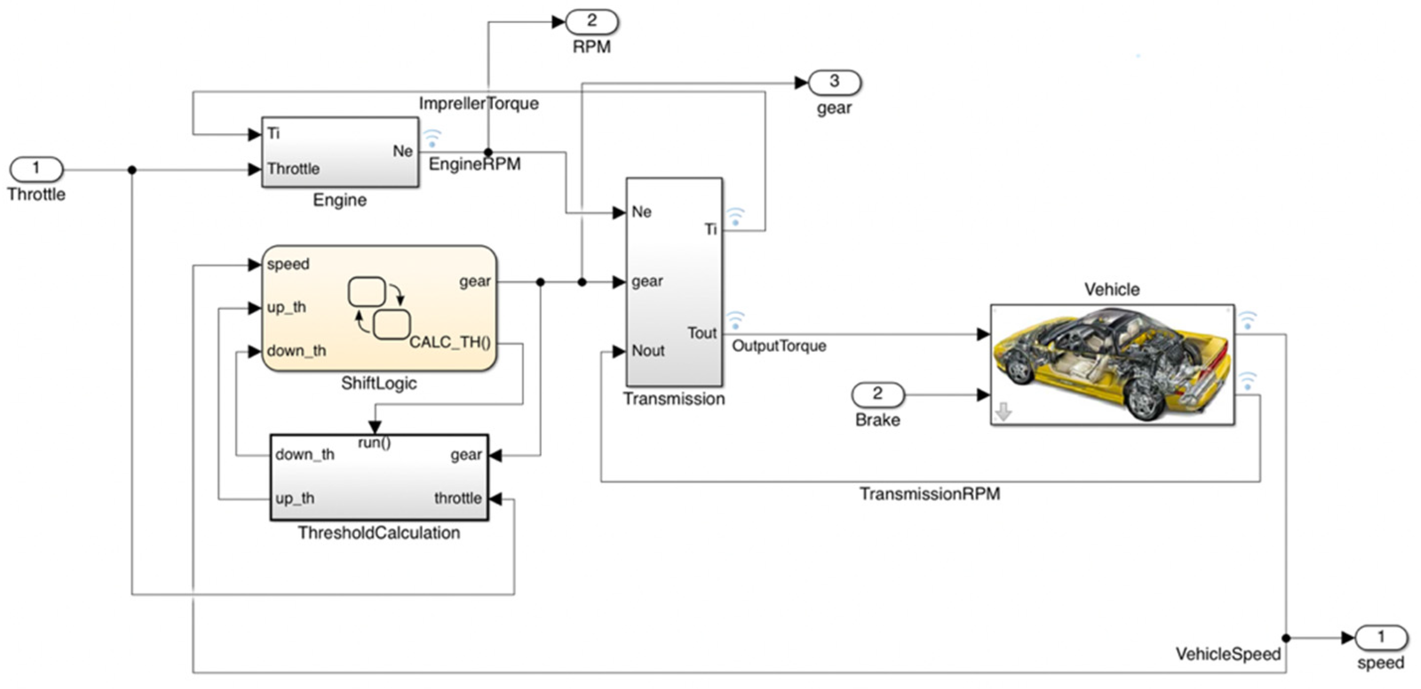
Falsification of the Cyber-physical system helps to discover defect-leading system parameters (i.e., counterexamples) to system specification, thereby enabling effective fault detection. The input with a minimal robustness (counterexample) is a good candidate to violate the specification. Here, we consider the Automatic Transmission example consisting of a Simulink^®/Stateflow™ model of an automatic transmission controller [112]. Figure 11 shows the corresponding top level Simulink model. The model has two input signals (the throttle and the brake). These signals represent the user’s throttle input through the accelerator pedal and the brake input. There are two outputs that represent the speed of the vehicle v (kmph) and the speed of the engine ω (RPM).

6.1. The Problem

We are interested in finding if the system always satisfies the temporal property ${\phi }_1^{AT}$: the speed should always remain below $\overline{v}$ kmph and the engine speed should remain below $\overline{\omega }$ RPM. In other words, the engine and the vehicle speed never reach $\overline{\omega }$ and $\overline{v}$, respectively. The requirement is specified in formal temporal logic specification and described by means of Signal Temporal Logic (STL) formulae given by:

$${\phi }_1^{AT}\left(\overline{v},\overline{\omega } \right)=G ((v<\overline{v}) \wedge (\omega <\overline{\omega }))$$

To violate this property, we search for input signals that cause the vehicle speed or the engine RPM to exceed their prescribed limits. In this work, we consider $\overline{v}$ $=120$ kmph and $\overline{\omega }=4500$ RPM. The total simulation time is T = 30 s.

Usually, given a formula $\phi$, the robustness of a trace $x$ w.r.t $\phi$ is defined as a real-valued quantity denoted $r : R\left(x, \phi \right)$. It is a measure of satisfaction of the trace w.r.t the property such that negative values of robustness indicate that the trace satisfies the negation of the property (if $r<0$, then $x \models \neg \phi$). The falsification approach is a simple optimization problem of minimizing the objective function over the decision variables z (that define the input signal(s)) such that the resulting trace $x$ has a negative value of robustness: find z such that $R\left(x, \phi \right)<0$. Here, the robustness is treated as the objective function which is minimized using various meta-heuristic approaches.

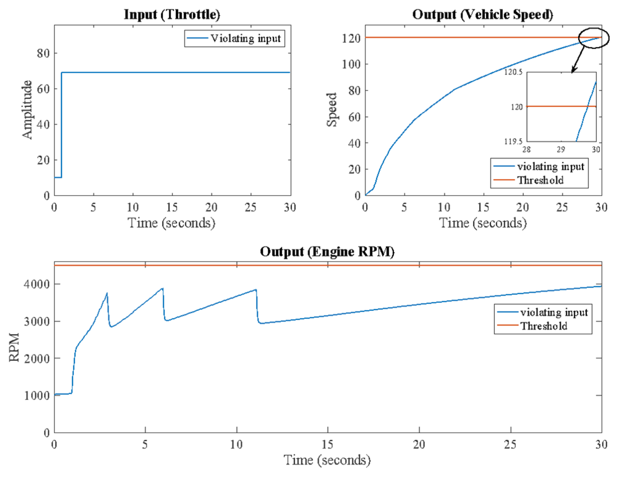
6.2. Simulation Results

We use the MoonLight tool (developed to monitor temporal and spatial-temporal properties of Cyber-Physical systems) [113] to find a counterexample for ${\phi }_1^{AT}$. Since we need robustness value for solving the optimization problem, we consider the quantitative semantics (or the minmax semantics) in this work. We try to falsify the STL formula ${\phi }_1^{AT}$ by taking the Brake input (kept constant = 0) and taking throttle i.e., input signal $u\left(t\right)$ as a step signal. We consider the throttle input as a step signal defined by the step time, the initial value and the final value. Moreover, we utilize BCA to solve the optimization problem and compare its performance with three well-known meta-heuristic techniques: GA, DE and PSO. The parameter settings for these algorithms are provided in Table 4.

Using the MoonLight tool, we obtain counterexamples by each optimization algorithm. Figure 12 shows the input throttle and the output speed and RPM corresponding to the counterexample for ${\phi }_1^{AT}$ obtained by BCA. The obtained counterexample corresponds to the input with (step time, initial value, final value) = (1, 10, 69). The robustness values acquired by BCA and other algorithms are tabulated in

Table 18. Results for the falsification problem of the automatic transmission controller system.

Approach	Robustness Value
BCA	−0.3564
PSO	−0.7236
GA	−1.6134
DE	−1.7380

. The results reveal that the proposed BCA is competitive enough for solving the falsification problem of Cyber-physical systems, demonstrating its applicability in real-world optimization problems.

Altogether, the results of this work validate that the proposed BCA serves as a powerful and reliable substitute to the existing meta-heuristic approaches.

7. Conclusions and Future Directions

This paper presented a novel bio-inspired population-based optimization algorithm called Blood Coagulation Algorithm (BCA). The proposed BCA mimics the process of blood coagulation in the human body. To investigate the performance of the proposed optimizer, we performed an extensive study on 23 mathematical benchmark functions and utilized 12 state-of-the-art algorithms for comparison. The intensification, diversification, local optima avoidance, and convergence behavior of BCA was investigated using unimodal and multimodal functions. We also analyzed the computational (time and space) complexity of BCA. The simulation and statistical results show that BCA is competitive with other well-regarded algorithms. Besides, the reliable performance of BCA for the high-dimensional functions paves the way for researchers to explore its applicability to diverse optimization tasks. Further, the analysis of six constrained and unconstrained engineering design tasks also demonstrated that BCA provided very competitive and outstanding results against other meta-heuristic algorithms. Moreover, the applicability of BCA on real world problems was also tested by employing it for the falsification of Cyber-Physical Systems. On the whole, it can be identified and may be asserted that BCA confirms its proficiency over other powerful meta-heuristic algorithms and is worth applying to solve other benchmark and real-world problems.

Numerous research directions can be proposed for future works. It would be interesting to extend BCA and develop its binary version, which could be a useful contribution to tackle real-world applications. Further, the extension of BCA to deal with multi-objective along with many-objective optimization problems would be noteworthy and can also be addressed in future works. Also, the performance of BCA with different constraint handling approaches for solving constrained optimization problems is worth researching. The capability of BCA to deal with highly constrained problems also needs to be explored. Further research is to be undertaken to check the effectiveness of the proposed algorithm in complex real-life applications (with complex search spaces) for handling various problems in multidisciplinary areas. In this work, we propose a very simple BCA with few mechanisms for intensification and diversification. Hence, the inclusion of other mechanisms (such as evolutionary updating structures, and chaos-based updating strategy) would be useful for future works.

References

- Fausto, F.; Reyna-Orta, A.; Cuevas, E.; Andrade, G.; Perez-Cisneros, M. From ants to whales: Metaheuristics for all tastes. Artif. Intell. Rev. 2019, 53, 753–810. [Google Scholar] [CrossRef]
- Boussaïd, I.; Lepagnot, J.; Siarry, P. A survey on optimization metaheuristics. Inf. Sci. 2013, 237, 82–117. [Google Scholar] [CrossRef]
- Holland, J.H. Genetic Algorithms. Sci. Am. 1992, 267, 66–73. Available online: https://www.jstor.org/stable/24939139 (accessed on 2 August 2021). [CrossRef]
- Koza, J.R. Genetic programming as a means for programming computers by natural selection. Stat. Comput. 1994, 4, 87–112. [Google Scholar] [CrossRef]
- Lampinen, J.; Storn, R. Differential Evolution. In New Optimization Techniques in Engineering. Studies in Fuzziness and Soft Computing; Springer: Berlin/Heidelberg, Germany, 2004; pp. 123–166. [Google Scholar]
- Simon, D. Biogeography-Based Optimization. IEEE Trans. Evol. Comput. 2008, 12, 702–713. [Google Scholar] [CrossRef] [Green Version]
- Bäck, T.; Bäck, T.; Hoffmeister, F.; Schwefel, H.-P. A Survey of Evolution Strategies. 1991. Available online: http://citeseerx.ist.psu.edu/viewdoc/summary?doi=10.1.1.42.3375 (accessed on 2 August 2021).
- Kennedy, J.; Eberhart, R. Particle swarm optimization. In Proceedings of the ICNN’95—International Conference on Neural Networks, Perth, Australia, 27 November–1 December 1995; pp. 1942–1948. [Google Scholar] [CrossRef]
- Mirjalili, S.; Mirjalili, S.M.; Lewis, A. Grey Wolf Optimizer. Adv. Eng. Softw. 2014, 69, 46–61. [Google Scholar] [CrossRef] [Green Version]
- Mirjalili, S.; Lewis, A. The Whale Optimization Algorithm. Adv. Eng. Softw. 2016, 95, 51–67. [Google Scholar] [CrossRef]
- Arora, S.; Singh, S. Butterfly optimization algorithm: A novel approach for global optimization. Soft Comput. 2018, 23, 715–734. [Google Scholar] [CrossRef]
- Heidari, A.A.; Mirjalili, S.; Faris, H.; Aljarah, I.; Mafarja, M.; Chen, H. Harris hawks optimization: Algorithm and applications. Future Gener. Comput. Syst. 2019, 97, 849–872. [Google Scholar] [CrossRef]
- Gandomi, A.H.; Yang, X.-S.; Alavi, A.H. Cuckoo search algorithm: A metaheuristic approach to solve structural optimization problems. Eng. Comput. 2011, 29, 17–35. [Google Scholar] [CrossRef]
- Mirjalili, S. Moth-flame optimization algorithm: A novel nature-inspired heuristic paradigm. Knowl.-Based Syst. 2015, 89, 228–249. [Google Scholar] [CrossRef]
- Yang, X.-S.; Karamanoglu, M.; He, X. Flower pollination algorithm: A novel approach for multiobjective optimization. Eng. Optim. 2013, 46, 1222–1237. [Google Scholar] [CrossRef] [Green Version]
- Gandomi, A.H.; Yang, X.-S.; Alavi, A.H. Mixed variable structural optimization using Firefly Algorithm. Comput. Struct. 2011, 89, 2325–2336. [Google Scholar] [CrossRef]
- Mirjalili, S.; Gandomi, A.H.; Mirjalili, S.Z.; Saremi, S.; Faris, H.; Mirjalili, S.M. Salp Swarm Algorithm: A bio-inspired optimizer for engineering design problems. Adv. Eng. Softw. 2017, 114, 163–191. [Google Scholar] [CrossRef]
- Blum, C. Ant colony optimization: Introduction and recent trends. Phys. Life Rev. 2005, 2, 353–373. [Google Scholar] [CrossRef] [Green Version]
- Gandomi, A.H.; Alavi, A.H. Krill herd: A new bio-inspired optimization algorithm. Commun. Nonlinear Sci. Numer. Simul. 2012, 17, 4831–4845. [Google Scholar] [CrossRef]
- Singh, H.; Singh, B.; Kaur, M. An improved elephant herding optimization for global optimization problems. Eng. Comput. 2021, 1–33. [Google Scholar] [CrossRef]
- Dhiman, G. ESA: A hybrid bio-inspired metaheuristic optimization approach for engineering problems. Eng. Comput. 2019, 37, 323–353. [Google Scholar] [CrossRef]
- Kirkpatrick, S.; Gelatt, C.D.; Vecchi, M.P. Optimization by Simulated Annealing. Science 1983, 220, 671–680. [Google Scholar] [CrossRef]
- Rashedi, E.; Nezamabadi-Pour, H.; Saryazdi, S. GSA: A Gravitational Search Algorithm. Inf. Sci. 2009, 179, 2232–2248. [Google Scholar] [CrossRef]
- Hatamlou, A. Black hole: A new heuristic optimization approach for data clustering. Inf. Sci. 2013, 222, 175–184. [Google Scholar] [CrossRef]
- Mirjalili, S. SCA: A Sine Cosine Algorithm for solving optimization problems. Knowl.-Based Syst. 2016, 96, 120–133. [Google Scholar] [CrossRef]
- Erol, O.K.; Eksin, I. A new optimization method: Big Bang–Big Crunch. Adv. Eng. Softw. 2006, 37, 106–111. [Google Scholar] [CrossRef]
- Eskandar, H.; Sadollah, A.; Bahreininejad, A.; Hamdi, M. Water cycle algorithm—A novel metaheuristic optimization method for solving constrained engineering optimization problems. Comput. Struct. 2012, 110–111, 151–166. [Google Scholar] [CrossRef]
- Yadav, A.A. AEFA: Artificial electric field algorithm for global optimization. Swarm Evol. Comput. 2019, 48, 93–108. [Google Scholar] [CrossRef]
- Gandomi, A.H.; Gandomi, A.H. Interior search algorithm (ISA): A novel approach for global optimization. ISA Trans. 2014, 53, 1168–1183. [Google Scholar] [CrossRef] [PubMed]
- Sadollah, A.; Bahreininejad, A.; Eskandar, H.; Hamdi, M. Mine blast algorithm: A new population based algorithm for solving constrained engineering optimization problems. Appl. Soft Comput. 2013, 13, 2592–2612. [Google Scholar] [CrossRef]
- Geem, Z.W.; Kim, J.H.; Loganathan, G. A new heuristic optimization algorithm: Harmony search. Simulation 2001, 76, 60–68. [Google Scholar] [CrossRef]
- Atashpaz-Gargari, E.; Lucas, C. Imperialist competitive algorithm: An algorithm for optimization inspired by imperialistic competition. In Proceedings of the 2007 IEEE Congress on Evolutionary Computation, Singapore, 25–28 September 2007. [Google Scholar] [CrossRef]
- Rao, R.V.; Savsani, V.J.; Vakharia, D.P. Teaching–learning-based optimization: A novel method for constrained mechanical design optimization problems. Comput. Aided Des. 2011, 43, 303–315. [Google Scholar] [CrossRef]
- Moosavian, N.; Roodsari, B.K. Soccer league competition algorithm: A novel meta-heuristic algorithm for optimal design of water distribution networks. Swarm Evol. Comput. 2014, 17, 14–24. [Google Scholar] [CrossRef]
- Ghorbani, N.; Babaei, E. Exchange market algorithm. Appl. Soft Comput. 2014, 19, 177–187. [Google Scholar] [CrossRef]
- Kumar, M.; Kulkarni, A.; Satapathy, S.C. Socio evolution & learning optimization algorithm: A socio-inspired optimization methodology. Future Gener. Comput. Syst. 2018, 81, 252–272. [Google Scholar] [CrossRef]
- Črepinšek, M.; Liu, S.-H.; Mernik, M. Exploration and exploitation in evolutionary algorithms. ACM Comput. Surv. 2013, 45, 1–33. [Google Scholar] [CrossRef]
- Wolpert, D.H.; Macready, W.G. No free lunch theorems for optimization. IEEE Trans. Evol. Comput. 1997, 1, 67–82. [Google Scholar] [CrossRef] [Green Version]
- Chamarthy, S. Normal Coagulation and Hemostasis. Pathobiol. Hum. Dis. Dyn. Encycl. Dis. Mech. 2014, 2014, 1544–1552. [Google Scholar] [CrossRef]
- Garmo, C.; Bajwa, T.; Burns, B. Physiology, Clotting Mechanism. StatPearls. 2020. Available online: https://www.ncbi.nlm.nih.gov/books/NBK507795/ (accessed on 22 July 2021).
- Davie, E.W.; Ratnoff, O.D. Waterfall Sequence for Intrinsic Blood Clotting. Science 1964, 145, 1310–1312. [Google Scholar] [CrossRef]
- Macfarlane, R.G. An Enzyme Cascade in the Blood Clotting Mechanism, and its Function as a Biochemical Amplifier. Nature 1964, 202, 498–499. [Google Scholar] [CrossRef]
- Monroe, D.M., 3rd; Hoffman, M. A Cell-based Model of Hemostasis. Thromb. Haemost. 2001, 85, 958–965. [Google Scholar] [CrossRef] [Green Version]
- Ferreira, C.N.; Sousa, M.D.O.; Dusse, L.; Carvalho, M.D.G. O novo modelo da cascata de coagulação baseado nas superfícies celulares e suas implicações. Rev. Bras. Hematol. Hemoter. 2010, 32, 416–421. [Google Scholar] [CrossRef] [Green Version]
- Oakley, C.; Larjava, H. Hemostasis, coagulation, and complications. Endod. Top. 2011, 24, 4–25. [Google Scholar] [CrossRef]
- Jesty, J.; Beltrami, E. Positive Feedbacks of Coagulation. Arter. Thromb. Vasc. Biol. 2005, 25, 2463–2469. [Google Scholar] [CrossRef]
- Askari, Q.; Younas, I.; Saeed, M. Political Optimizer: A novel socio-inspired meta-heuristic for global optimization. Knowl.-Based Syst. 2020, 195, 105709. [Google Scholar] [CrossRef]
- Storn, R.; Price, K. Differential Evolution—A Simple and Efficient Heuristic for global Optimization over Continuous Spaces. J. Glob. Optim. 1997, 11, 341–359. [Google Scholar] [CrossRef]
- Bonabeau, M.E.; Dorigo, G. Theraulaz, Swarm Intelligence: From Natural to Artificial Isystems; Oxford University Press: Oxford, UK, 1999. [Google Scholar]
- Yang, X.-S.; Gandomi, A.H. Bat algorithm: A novel approach for global engineering optimization. Eng. Comput. 2012, 29, 464–483. [Google Scholar] [CrossRef] [Green Version]
- Abualigah, L.; Diabat, A.; Mirjalili, S.; Elaziz, M.A.; Gandomi, A.H. The Arithmetic Optimization Algorithm. Comput. Methods Appl. Mech. Eng. 2021, 376, 113609. [Google Scholar] [CrossRef]
- Derrac, J.; García, S.; Molina, D.; Herrera, F. A practical tutorial on the use of nonparametric statistical tests as a methodology for comparing evolutionary and swarm intelligence algorithms. Swarm Evol. Comput. 2011, 1, 3–18. [Google Scholar] [CrossRef]
- Coello, C.A.C. Theoretical and numerical constraint-handling techniques used with evolutionary algorithms: A survey of the state of the art. Comput. Methods Appl. Mech. Eng. 2002, 191, 1245–1287. [Google Scholar] [CrossRef]
- Ragsdell, K.M.; Phillips, D.T. Optimal Design of a Class of Welded Structures Using Geometric Programming. J. Eng. Ind. 1976, 98, 1021–1025. [Google Scholar] [CrossRef]
- Deb, K. Optimal design of a welded beam via genetic algorithms. AIAA J. 1991, 29, 2013–2015. [Google Scholar] [CrossRef]
- Coello, C.C. Use of a self-adaptive penalty approach for engineering optimization problems. Comput. Ind. 2000, 41, 113–127. [Google Scholar] [CrossRef]
- Lee, K.S.; Geem, Z.W. A new structural optimization method based on the harmony search algorithm. Comput. Struct. 2004, 82, 781–798. [Google Scholar] [CrossRef]
- Mezura-Montes, E.; Coello, C.C. A Simple Multimembered Evolution Strategy to Solve Constrained Optimization Problems. IEEE Trans. Evol. Comput. 2005, 9, 1–17. [Google Scholar] [CrossRef]
- Huang, F.-Z.; Wang, L.; He, Q. An effective co-evolutionary differential evolution for constrained optimization. Appl. Math. Comput. 2007, 186, 340–356. [Google Scholar] [CrossRef]
- Mirjalili, S.; Mirjalili, S.M.; Hatamlou, A. Multi-Verse Optimizer: A nature-inspired algorithm for global optimization. Neural Comput. Appl. 2015, 27, 495–513. [Google Scholar] [CrossRef]
- Mezura-Montes, E.; Coello, C.A.C. An empirical study about the usefulness of evolution strategies to solve constrained optimization problems. Int. J. Gen. Syst. 2008, 37, 443–473. [Google Scholar] [CrossRef]
- Hedar, A.-R.; Fukushima, M. Derivative-Free Filter Simulated Annealing Method for Constrained Continuous Global Optimization. J. Glob. Optim. 2006, 35, 521–549. [Google Scholar] [CrossRef]
- He, Q.; Wang, L. An effective co-evolutionary particle swarm optimization for constrained engineering design problems. Eng. Appl. Artif. Intell. 2007, 20, 89–99. [Google Scholar] [CrossRef]
- Cagnina, L.C.; Esquivel, S.C.; Coello, C.A.C. Solving Engineering Optimization Problems with the Simple Constrained Particle Swarm Optimizer. Informatica 2008, 32, 319–326. [Google Scholar]
- Mezura-Montes, E.; Coello, C.C.; Velázquez-Reyes, J.; Muñoz-Dávila, L. Multiple trial vectors in differential evolution for engineering design. Eng. Optim. 2007, 39, 567–589. [Google Scholar] [CrossRef]
- Karaboga, D.; Basturk, B. On the performance of artificial bee colony (ABC) algorithm. Appl. Soft Comput. 2008, 8, 687–697. [Google Scholar] [CrossRef]
- Kaveh, A.; Talatahari, S. An improved ant colony optimization for constrained engineering design problems. Eng. Comput. 2010, 27, 155–182. [Google Scholar] [CrossRef]
- Coello, C.A.C.; Becerra, R.L. Efficient evolutionary optimization through the use of a cultural algorithm. Eng. Optim. 2004, 36, 219–236. [Google Scholar] [CrossRef]
- Yuan, Q.; Qian, F. A hybrid genetic algorithm for twice continuously differentiable NLP problems. Comput. Chem. Eng. 2010, 34, 36–41. [Google Scholar] [CrossRef]
- Kohli, M.; Arora, S. Chaotic grey wolf optimization algorithm for constrained optimization problems. J. Comput. Des. Eng. 2017, 5, 458–472. [Google Scholar] [CrossRef]
- Krohling, R.A.; Coelho, L. Coevolutionary Particle Swarm Optimization Using Gaussian Distribution for Solving Constrained Optimization Problems. IEEE Trans. Syst. Man Cybern. Part B 2006, 36, 1407–1416. [Google Scholar] [CrossRef] [PubMed]
- Coello, C.A.C.; Montes, E.M. Constraint-handling in genetic algorithms through the use of dominance-based tournament selection. Adv. Eng. Inform. 2002, 16, 193–203. [Google Scholar] [CrossRef]
- Yang, X.-S.; Deb, S. Cuckoo Search via Lvy flights. In Proceedings of the 2009 World Congress Nature & Biologically Inspired Computing (NaBIC), Coimbatore, India, 9–11 December 2009; pp. 210–214. [Google Scholar] [CrossRef]
- Yang, X.-S. A New Metaheuristic Bat-Inspired Algorithm. Nature Inspired Cooperative Strategies for Optimization (NICSO 2010). In Studies in Computational Intelligence; Springer: Berlin/Heidelberg, Germany, 2010; Volume 284, pp. 65–74. [Google Scholar]
- Braik, M.; Sheta, A.; Al-Hiary, H. A novel meta-heuristic search algorithm for solving optimization problems: Capuchin search algorithm. Neural Comput. Appl. 2020, 33, 2515–2547. [Google Scholar] [CrossRef]
- Liu, H.; Cai, Z.; Wang, Y. Hybridizing particle swarm optimization with differential evolution for constrained numerical and engineering optimization. Appl. Soft Comput. 2010, 10, 629–640. [Google Scholar] [CrossRef]
- Mohamed, A.; Sabry, H.Z. Constrained optimization based on modified differential evolution algorithm. Inf. Sci. 2012, 194, 171–208. [Google Scholar] [CrossRef]
- Wang, L.; Li, L.-P. An effective differential evolution with level comparison for constrained engineering design. Struct. Multidiscip. Optim. 2009, 41, 947–963. [Google Scholar] [CrossRef]
- Hamza, F.; Abderazek, H.; Lakhdar, S.; Ferhat, D.; Yildiz, A.R. Optimum design of cam-roller follower mechanism using a new evolutionary algorithm. Int. J. Adv. Manuf. Technol. 2018, 99, 1267–1282. [Google Scholar] [CrossRef]
- Abderazek, H.; Ferhat, D.; Ivana, A. Adaptive mixed differential evolution algorithm for bi-objective tooth profile spur gear optimization. Int. J. Adv. Manuf. Technol. 2016, 90, 2063–2073. [Google Scholar] [CrossRef]
- Lee, K.S.; Geem, Z.W. A new meta-heuristic algorithm for continuous engineering optimization: Harmony search theory and practice. Comput. Methods Appl. Mech. Eng. 2005, 194, 3902–3933. [Google Scholar] [CrossRef]
- Mirjalili, S. Dragonfly algorithm: A new meta-heuristic optimization technique for solving single-objective, discrete, and multi-objective problems. Neural Comput. Appl. 2015, 27, 1053–1073. [Google Scholar] [CrossRef]
- Akay, B.; Karaboga, D. Artificial bee colony algorithm for large-scale problems and engineering design optimization. J. Intell. Manuf. 2010, 23, 1001–1014. [Google Scholar] [CrossRef]
- He, S.; Prempain, E.; Wu, Q.H. An improved particle swarm optimizer for mechanical design optimization problems. Eng. Optim. 2004, 36, 585–605. [Google Scholar] [CrossRef]
- Garg, H. Solving structural engineering design optimization problems using an artificial bee colony algorithm. J. Ind. Manag. Optim. 2014, 10, 777–794. [Google Scholar] [CrossRef]
- Zahara, E.; Kao, Y.-T. Hybrid Nelder–Mead simplex search and particle swarm optimization for constrained engineering design problems. Expert Syst. Appl. 2009, 36, 3880–3886. [Google Scholar] [CrossRef]
- He, Q.; Wang, L. A hybrid particle swarm optimization with a feasibility-based rule for constrained optimization. Appl. Math. Comput. 2006, 186, 1407–1422. [Google Scholar] [CrossRef]
- Coelho, L.D.S. Gaussian quantum-behaved particle swarm optimization approaches for constrained engineering design problems. Expert Syst. Appl. 2010, 37, 1676–1683. [Google Scholar] [CrossRef]
- Kaveh, A.; Talatahari, S. A novel heuristic optimization method: Charged system search. Acta Mech. 2010, 213, 267–289. [Google Scholar] [CrossRef]
- Arora, J. Introduction to Optimum Design; Elsevier Academic Press: Amsterdam, The Netherlands, 2004. [Google Scholar]
- Zhang, M.; Luo, W.; Wang, X. Differential evolution with dynamic stochastic selection for constrained optimization. Inf. Sci. 2008, 178, 3043–3074. [Google Scholar] [CrossRef]
- Wang, Y.; Cai, Z.; Zhou, Y.; Fan, Z. Constrained optimization based on hybrid evolutionary algorithm and adaptive constraint-handling technique. Struct. Multidiscip. Optim. 2008, 37, 395–413. [Google Scholar] [CrossRef]
- Saremi, S.; Mirjalili, S.; Lewis, A. Grasshopper Optimisation Algorithm: Theory and application. Adv. Eng. Softw. 2017, 105, 30–47. [Google Scholar] [CrossRef] [Green Version]
- Tsai, J.-F. Global optimization of nonlinear fractional programming problems in engineering design. Eng. Optim. 2005, 37, 399–409. [Google Scholar] [CrossRef]
- Ray, T.; Saini, P. Engineering Design Optimization Using a Swarm with an Intelligent Information Sharing among Individuals. Eng. Optim. 2001, 33, 735–748. [Google Scholar] [CrossRef]
- Mezura-Montes, E.; Velazquez-Reyes, J.; Coello, C.C. Modified Differential Evolution for Constrained Optimization. Int. Conf. Evol. Comput. 2006, 2006, 25–32. [Google Scholar] [CrossRef]
- Baykasoğlu, A.; Akpinar, Ş. Weighted Superposition Attraction (WSA): A swarm intelligence algorithm for optimization problems–Part 2: Constrained optimization. Appl. Soft Comput. 2015, 37, 396–415. [Google Scholar] [CrossRef]
- Czerniak, J.M.; Zarzycki, H.; Ewald, D. AAO as a new strategy in modeling and simulation of constructional problems optimization. Simul. Model. Pract. Theory 2017, 76, 22–33. [Google Scholar] [CrossRef]
- Ben Guedria, N. Improved accelerated PSO algorithm for mechanical engineering optimization problems. Appl. Soft Comput. 2016, 40, 455–467. [Google Scholar] [CrossRef]
- Baykasoglu, A.; Ozsoydan, F.B. Adaptive firefly algorithm with chaos for mechanical design optimization problems. Appl. Soft Comput. 2015, 36, 152–164. [Google Scholar] [CrossRef]
- Ray, T.; Liew, K.M. Society and civilization: An optimization algorithm based on the simulation of social behavior. IEEE Trans. Evol. Comput. 2003, 7, 386–396. [Google Scholar] [CrossRef]
- Sandgren, E. Nonlinear Integer and Discrete Programming in Mechanical Design Optimization. J. Mech. Des. 1990, 112, 223–229. [Google Scholar] [CrossRef]
- Gandomi, A.H.; Yun, G.J.; Yang, X.-S.; Talatahari, S. Chaos-enhanced accelerated particle swarm optimization. Commun. Nonlinear Sci. Numer. Simul. 2013, 18, 327–340. [Google Scholar] [CrossRef]
- Deb, K.; Deb, K.; Goyal, M. A Combined Genetic Adaptive Search (GeneAS) for Engineering Design. Comput. Sci. Inform. 1996, 26, 30–45. Available online: http://citeseerx.ist.psu.edu/viewdoc/summary?doi=10.1.1.27.767 (accessed on 23 July 2021).
- Parsopoulos, K.E.; Vrahatis, M.N. Unified Particle Swarm Optimization for Solving Constrained Engineering Optimization Problems. Lect. Notes Comput. Sci. 2005, 3612, 582–591. [Google Scholar] [CrossRef] [Green Version]
- Loh, H.T.; Papalambros, P.Y. A Sequential Linearization Approach for Solving Mixed-Discrete Nonlinear Design Optimization Problems. J. Mech. Des. 1991, 113, 325–334. [Google Scholar] [CrossRef]
- Zhang, C.; Wang, H.-P. Mixed-Discrete Nonlinear Optimization with Simulated Annealing. Eng. Optim. 1993, 21, 277–291. [Google Scholar] [CrossRef]
- Kannan, B.K.; Kramer, S.N. An Augmented Lagrange Multiplier Based Method for Mixed Integer Discrete Continuous Optimization and Its Applications to Mechanical Design. J. Mech. Des. 1994, 116, 405–411. [Google Scholar] [CrossRef]
- Cao, Y.; Wu, Q. Evolutionary Programming. In Proceedings of the IEEE International Conference on Evolutionary Computation (ICEC ‘97), Indianapolis, IN, USA, 13–16 April 1997. [Google Scholar] [CrossRef]
- Wu, S.-J.; Chow, P.-T. Genetic Algorithms for Nonlinear Mixed Discrete-Integer Optimization Problems via Meta-Genetic Parameter Optimization. Eng. Optim. 1995, 24, 137–159. [Google Scholar] [CrossRef]
- Fu, J.-F.; Fenton, R.G.; Cleghorn, W.L. A mixed integer-discrete-continuous programming method and its application to engineering design optimization. Eng. Optim. 1991, 17, 263–280. [Google Scholar] [CrossRef]
- Zhao, Q.; Krogh, B.; Hubbard, P. Generating test inputs for embedded control systems. IEEE Control. Syst. 2003, 23, 49–57. [Google Scholar] [CrossRef]
- Bartocci, E.; Bortolussi, L.; Loreti, M.; Nenzi, L.; Silvetti, S. MoonLight: A Lightweight Tool for Monitoring Spatio-Temporal Properties. Lect. Notes Comput. Sci. 2020, 12399, 417–428. [Google Scholar] [CrossRef]
Figure 1.
Schematic of Hemostasis illustrating the general steps of blood clotting.
Figure 2.
Different updating phases of BCA.
Figure 3.
Search space of the unimodal benchmark functions (2-D view).
Figure 4.
Search space of the multimodal benchmark functions (2-D view).
Figure 5.
Search space of the fixed-dimension multimodal benchmark functions (2-D view).
Figure 6.
Illustration of the search history of thrombocytes. For visualization, we consider the 2D version of the benchmark functions.
Figure 7.
Trajectories of some randomly chosen thrombocytes for some of the benchmark functions (We consider the 2D version of the benchmark functions).
Figure 8.
Comparison of convergence curves of BCA and few eminent algorithms for some of the benchmark functions.
Figure 9.
Scalability analysis of the proposed BCA for different dimensions of the benchmark functions .
Figure 10.
Schematic views of the engineering design problems considered in this work. (a) Welded beam design (Image taken from [27]); (b) Pressure vessel design (Image taken from [27] ); (c) Tension/compression spring design (Image taken from [11]); (d) Three-bar truss design (Image taken from [12]); (e) Speed reducer design (Image taken from [51]); (f) Gear train design.
Figure 11.
The automatic transmission system Simulink®/Stateflow™ model.
Figure 12.
Input and output plots for the counterexample for found by BCA.