Algebraic Analysis of Variants of Multi-State k-out-of-n Systems

Abstract

We apply the algebraic reliability method to the analysis of several variants of multi-state k-out-of-n systems. We describe and use the reliability ideals of multi-state consecutive k-out-of-n systems with and without sparse, and show the results of computer experiments on these kinds of systems. We also give an algebraic analysis of weighted multi-state k-out-of-n systems and show that this provides an efficient algorithms for the computation of their reliability.

1. Introduction

The usual approach to system reliability assumes that the system and its components can only be in one of two states, failure and working. However, many systems and equipments in engineering applications exhibit multiple performance or capacity levels and therefore cannot be adequately modeled by binary methods. For such non-binary situations, several models of multi-state reliability analysis have been proposed in the literature, e.g., [1,2,3,4,5]. In multi-state (MS) systems both the system and its components can be in any of a discrete set of states that indicates different levels of performance. This allows the modeling of a wide variety of situations and is an area of intense research and practice.

Among the most important binary systems are k-out-of-n systems and its variants, e.g., linear consecutive, circular consecutive, weighted, etc. These systems model redundancy in fault-tolerant systems and are used in many applications of a very different practical nature [1]. Multi-state versions of k-out-of-n systems have been proposed in the literature and several methods are used for their reliability analysis. The generalized MS k-out-of-n:G system model was proposed in [6]. Since then, significant efforts have been made in the analysis of such systems and to produce efficient algorithms for their reliability computation, see [7] and the references therein for a complete account.

In recent years, several models have been proposed to describe practical situations that cannot be modeled by usual k-out-of-n systems. For instance, the MS consecutive k-out-of-n model was proposed in [8], weighted multi-state k-out-of-n systems were studied in [9] and sparsely connected homogeneous multi-state consecutive k-out-of-n:G systems were recently proposed in [10].

For binary and multi-state systems, several algebraic methodologies have been suggested that allow the efficient analysis of their structure and reliability. In the case that the structure function of the system can be analyzed in recursive terms (for instance, series-parallel systems and others) the Universal Generating Function method has shown to be very flexible and efficient [2,3,11]. In case that the structure function does not have an easy to describe pattern, like in general networks, the algebraic method based on monomial ideals is an approach that also produces efficient algorithms [12,13,14,15]. This latter method has been used to analyze k-out-of-n systems and variants in the binary case [13,16] and the generalized multi-state version [17]. In summary, this method assigns for each level j of performance of the system a monomial ideal whose minimal generating set is in correspondence with the set of minimal working states of the system. The algebraic study of this ideal, in particular of its Hilbert series, provides a direct method for computing the j-reliability of the systems. A detailed account of this methodology can be seen in the above references.

In the present paper, we take advantage of the versatility of the algebraic method based on monomial ideals and apply it to the analysis of the reliability of recently proposed variants of multi-state k-out-of-n systems. Section 2 reviews the basic definitions and notations about coherent systems and the algebraic method. In Section 3, we analyze multi-state consecutive k-out-of-n systems, giving formulas and bounds for their reliability. Section 4 applies the algebraic method to the recently proposed sparsely connected homogeneous multi-state consecutive k-out-of-n:G system model. Finally, Section 5 is devoted to multi-state weighted k-out-of-n systems.

2. Basic Definitions

A system $\mathcal{S}$ consists of n components denoted by $c_i$ with $i\in \{1,\dots ,n\}$. At each moment in time, the system is in one of a discrete set of levels $S=\{0,1,\dots ,M\}$ indicating growing levels of performance. Each component $c_i$ of the system can be in one of a discrete set of levels $S_i=\{0,\dots ,M_i\}$. A state of a component is its level and a state of the system is given by an n-tuple of its components’ states. Given two states $s=(s_1,\dots ,s_n)$ and $t=(t_1,\dots ,t_n)$, we say that $s\ge t$ if $s_i\ge t_i$ for all $i=1,\dots ,n$ and, conversely, that $s\le t$ if $s_i\le t_i$ for all i. The level of performance of the system is determined in terms of the states of the components by a structure function $\Phi :S_1\times \cdots \times S_n⟶S$. The system $\mathcal{S}$ is said to be coherent if $\Phi$ is non-decreasing and each component is relevant to the system, i.e., for each component $c_i$ there exist a system state $s=(s_1,\dots ,s_n)$ and two different levels $j,k\in S_i$ such that $\Phi \left(s_{i,j}\right)\ne \Phi \left(s_{i,k}\right)$, where $s_{i,\ell }=(s_1,\dots ,s_{i-1},\ell ,s_{i+1},\dots ,s_n)$.

The levels of the system $\{0,\dots ,M\}$ indicate growing levels of performance, the system being in level 0 indicates that the system is failing, and level $j>i$ indicates that the system is performing at level j better than at level i. For each component $c_i$ and for each of its levels j, we denote by $p_{i,j}$ the probability that $c_i$ is performing at level $\ge j$. The j-reliability of $\mathcal{S}$, denoted by $R_j\left(\mathcal{S}\right)$ is the probability that $\mathcal{S}$ is performing at level $\ge j$; conversely, the j-unreliability of $\mathcal{S}$, denoted $U_j\left(\mathcal{S}\right)$, is $1-R_j\left(\mathcal{S}\right)$. A coherent system is given at level j by its set of j-working states, i.e., those tuples $(s_1,\dots ,s_n)\in S_1\times \cdots \times S_n$ such that $\Phi (s_1,\dots ,s_n)\ge j$. We say that a state $(s_1,\dots ,s_n)\in S_1\times \cdots \times S_n$ is a minimal j-working state or minimal j-path if $\Phi (s_1,\dots ,s_n)\ge j$ and $\Phi (t_1,\dots ,t_n)<j$ whenever all $t_i\le s_i$ and at least in one case the inequality is strict. We say that a state $(s_1,\dots ,s_n)\in S_1\times \cdots \times S_n$ is a minimal j-failure state or minimal j-cut if $\Phi (s_1,\dots ,s_n)<j$ and $\Phi (t_1,\dots ,t_n)\ge j$ whenever all $t_i\ge s_i$ and at least one of the inequalities is strict. These systems are usually denoted by :G (for good) in the literature. If instead of paths we consider cuts, then the sytems are denoted by :F (for fail).

Let $\mathcal{S}$ be a system with n components and let $j\in \{0,\dots ,M\}$ be one of the levels of the system. Let $F_j\left(\mathcal{S}\right)$ be the set of j-working states of the system and ${\overline{F}}_j\left(\mathcal{S}\right)$ the subset of minimal j-working states. Let us consider $P=\mathbf{k}[x_1,\dots ,x_n]$ a polynomial ring in n indeterminates where $\mathbf{k}$ denotes any field of characteristic 0. To each state $s=(s_1,\dots ,s_n)\in S_1\times \cdots \times S_n$ of $\mathcal{S}$ we associate the monomial $x^s=x_1^{s_1}\cdots x_n^{s_n}\in P$.

We denote by $pr\left(x^s\right)={\prod }_{i=1}^n{p}_{i,s_i}$ the probability that the system is in a state $\ge s$. In algebraic terms, having a state $t\ge s$ is equivalent to saying that the monomial $x^t$ is a multiple of $x^s$, i.e., $x^t$ is in $I=\langle x^s\rangle$, the ideal in P generated by the monomial $x^s$. Now we consider the probability that the system is in a state greater than or equal to at least one of the states in $\{{\mu }_1,\dots ,{\mu }_r\}$: this situation algebraically corresponds to the set of monomials $x^t$ belonging to the ideal $I=\langle x^{{\mu }_1},\dots ,x^{{\mu }_r}\rangle$. Thus we denote its probability by $pr\left(I\right)=pr\left({\bigcup }_{i=1}^r\langle x^{{\mu }_i}\rangle \right)$.

The ideal generated by the j-working states of $\mathcal{S}$ is denoted by $I_j\left(\mathcal{S}\right)$ and is called the j-reliability ideal of $\mathcal{S}$. For a monomial ideal there is a unique minimal monomial generating set, denoted $\mathrm{MinGens}\left(I\right)$. Due to the coherence property of $\mathcal{S}$, we have that $\mathrm{MinGens}\left(I_j\left(\mathcal{S}\right)\right)$ is the set of the monomials corresponding to the minimal j-paths of $\mathcal{S}$. The multigraded Hilbert series of an ideal provides a compact way to enumerate all monomials in a monomial ideal. The multigraded Hilbert series of an ideal $I\in P$, given by

$$H_I(x_1,\dots ,x_n)=\sum _{\mu \in {\mathbb{N}}^n}[x^{\mu }\in I]x^{\mu }=\sum _{i=1}^r{(-1)}^{i+1}\sum _{\left|\sigma \right|=i}\frac{\mathrm{lcm}\left(x^{{\mu }_s}\right|s\in \sigma )}{{\prod }_{j=1}^n(1-x_j)},$$

where the symbol $[x^{\mu }\in I]$ is equal to 1 if $x^{\mu }$ is in I and 0 otherwise. Let now $H{N}_I(x_1,\dots ,x_n)$ denote the numerator of the Hilbert series of the ideal I and let $\mathcal{S}$ be a coherent system. Let $pr\left(H{N}_{I_j\left(\mathcal{S}\right)}(x_1,\dots ,x_n)\right)$ denote the formal substitution of every $x^{\mu }$ by $pr\left(x^{\mu }\right)$ in the numerator of the multigraded Hilbert series of $I_j\left(\mathcal{S}\right)$, then we have that

$$R_j\left(\mathcal{S}\right)=pr\left(I_j\left(\mathcal{S}\right)\right)=pr\left(H{N}_{I_j\left(\mathcal{S}\right)}(x_1,\dots ,x_n)\right).$$

Hence, any way to obtain $H{N}_{I_j\left(\mathcal{S}\right)}(x_1,\dots ,x_n)$ gives us a way to compute $R_j\left(\mathcal{S}\right)$. One such way is by constructing a multigraded free resolution of I and read $HN\left(I\right)$ from the data in the resolution. This is the approach we use in our algorithms, for it provides compact forms of the inclusion-exclusion formulas and Bonferroni bounds. In particular, we use Mayer–Vietoris trees [18] as an efficient algorithm to obtain a compressed expression of $H{N}_{I_j\left(\mathcal{S}\right)}(x_1,\dots ,x_n)$.

3. Multi-State Consecutive $k$-out-of-$n$ Systems

A definition of consecutive multi-state k-out-of-n:F systems, in which k could take different values for different system levels was proposed in [8]. Under that definition, a possibly different number of consecutive components need to be below level j for the system to be below level j for different levels. The required number of consecutive component failures is thus dependent on the system level under consideration. The definition is formalized as follows

Definition 1.

An n-component multi-state system such that its structure function Φ satisfies that $\Phi \left(x\right)<j$ for $j=1,2,\dots ,M$ if at least $k_l$ consecutive components are in states below l for all $j\le l\le M$ is called a multi-state consecutive k-out-of-n:F system.

If $k_1\ge k_2\ge \cdots \ge k_M$ the system is called a decreasing multi-state consecutive k-out-of-n:F system. In this case, as j increases, the requirement on the number of consecutive components that must be below state j for the system to be below state level j also decreases.

If $k_1\le k_2\le \cdots \le k_M$, the system is an increasing multi-state consecutive k-out-of-n:F system. In this case, for the system to be below a higher state level j, a larger number of consecutive components must be below state j.

If all the $k_j$ are the same we say the system is a constant consecutive k-out-of-n:F system.

Example 1

([8] Example 2, [1] Example 12.16). Consider a three-component system where both the system and the components may be in one of three possible states: $0,1$ and 2 . The system is below state 2 if and only if at least one component is below state 2, i.e., $k_2=1$. The system is below state 1 if and only if at least two consecutive components are below state 1, i.e., $k_1=2$. This is a strictly decreasing multi-state consecutive k-out-of-n system. This system has a consecutive 1-out-of-3:F structure at system state level 2 and a consecutive 2-out-of-3:F structure at system state level 1.

Example 2

([8] Example 3, [1] Example 12.17). Consider a three-component system where both the system and the components may be in one of four possible states: $0,1,2$ and 3. The system is below state 3 if and only if the three components are below state 3. The system is below state 2 if and only if at least two consecutive components are below state 2 and the three components are below state 3. The system is below state 1 if and only if at least one component is below state 1, at least two consecutive components are below state 2, and at least three components are below state 3. The system in this example has a 3-out-of-3:F structure at system state 3, a consecutive 2-out-of-3:F structure at system state level 2, and a 1-out-of-3:F structure at system state level 1.

Given a structure function $\Phi$, its dual ${\Phi }^D$ with respect to $\mathbf{t}\in {\mathbb{N}}^n$ is given by (cf. [19], and see [20] for the case $\mathbf{t}=(1,\dots ,1)$, $M=1$)

$${\Phi }^D(s_1,\dots ,s_n)=M-\Phi \left((t_1-s_1,\dots ,t_n-s_n)\right).$$

(1)

In our case, we use $\mathbf{t}=(M,\dots ,M)$. This means that the dual system is in state $M-j$ or above if and only if the original system is in state j or below, and that for probability evaluation, the probability of the dual component ${\overline{c}}_i$ to be in state greater or equal to $M-j$ is the probability that the original component $c_i$ is at state lower than or equal to j. Observe that MS consecutive k-out-of-n:F systems are dual to consecutive k-out-of-n:G systems; this duality transforms increasing systems in decreasing ones and vice-versa. For the algebraic treatment of these systems we shall make use of their dual structure. We can treat the consecutive k-out-of-n:F structures at each level of our systems as consecutive k-out-of-n:G structures and take advantage of the ideal structure. In this setting, the system-to-ideal correspondence is clearer and more convenient.

Let $I_{k,n}$ be the reliability ideal of a binary consecutive k-out-of-n system, this ideal is given by

$$I_{k,n}=\langle x_1\cdots x_k,x_2\cdots x_{k+1},\dots ,x_{n-k+1}\cdots x_n\rangle .$$

The graded Betti numbers of $I_{k,n}$ can be recursively computed by the formulas given in [16], where ${\beta }_{i,j,k,n}$ indicates the i-th Betti number in degree j of the ideal $I_{k,n}$:

$$\begin{array}{ccc}\hfill {\beta }_{0,k,k,n}& =n-k+1,\hfill & \\ \hfill {\beta }_{1,k+1,k,n}& =n-k,\mathrm{for} k\ge \frac{n}{2},\hfill & \\ \hfill {\beta }_{1,k+1,k,n}& =1+{\beta }_{1,k+1,k,n-1},\mathrm{for} k<\frac{n}{2},\hfill & \\ \hfill {\beta }_{1,2k,k,n}& =n-2k+{\beta }_{1,2k,k,n-1},\mathrm{for} k<\frac{n}{2},\hfill & \\ \hfill {\beta }_{i,j,k,n}& ={\beta }_{i-2,j-k-1,k,n-k-1}+{\beta }_{i-1,j-k,k,n-k-1}+{\beta }_{i,j,k,n-1}\forall i\ge 2,\mathrm{for} k<\frac{n}{2}.\hfill & \end{array}$$

Let us denote by $I_{k,n,j}$ the monomial ideal given by the generators of $I_{k,n}$ in which each variable is raised to the j-th power

$$I_{k,n,j}=\langle x_1^j\cdots x_k^j,x_2^j\cdots x_{k+1}^j,\dots ,x_{n-k+1}^j\cdots x_n^j\rangle$$

Observe that for this ideal, the graded Betti numbers are given by

$${\beta }_{i,d,}\left(I_{k,n,j}\right)={\beta }_{i,\frac{d}{j}}\left(I_{k,n}\right).$$

An increasing or constant multi-state consecutive k-out-of-n:G system (i.e., a decreasing k-out-of-n:F system) works at level j if at least $k_j$ components work at level j or more, and these requirements do not overlap among the levels. Therefore, each level has a binary consecutive $k_j$-out-of-n structure and the j-th reliability ideal is given by

$${\overline{I}}_{k,n,j}=I_{k_j,n,j}$$

Example 3.

The system in Example 1 corresponds to a multi-state consecutive k-out-of-n:G system with $k_1=1,k_2=2$, hence the j-reliability ideals are given by   

$$\begin{array}{cc}\hfill {\overline{I}}_{k,n,1}=& \langle x,y,z\rangle ,\hfill \\ \hfill {\overline{I}}_{k,n,2}=& \langle x^2{y}^2,y^2{z}^2\rangle \hfill \end{array}$$

The case of decreasing MS consecutive k-out-of-n:G system (i.e., increasing MS consecutive k-out-of-n:F systems) is more complex. The main difficulty comes from the fact that multi-state decreasing consecutive k-out-of-n:G systems consist of a set of binary consecutive k-out-of-n structures connected by and operators to describe the conditions under which the system is in state j or above, and these individual structures are not embedded in one another. The system is in state j or above if there are $k_j$ consecutive components in state j or above and if there are $k_{j^{\prime }}$ consecutive components in state $j^{\prime }$ or above for each $j^{\prime }<j$. Since the system is decreasing, these conditions do not completely overlap.

Example 4.

The dual to the system in Example 2 is a decreasing multi-state consecutive k-out-of-n system such that $k_1=3$, $k_2=2$ and $k_3=1$. The system is in state 1 or above if at least three components are in state 1 or above; the system is in state 2 or above if at least 2 consecutive components are in state 2 or above and at least 3 components are in state 1 or above. Finally, the system is in state 3 if at least 1 component is in state 3 and at least 2 components are in state 2 or above and at least 3 components are in state 1 or above. This system consists of three binary consecutive k-out-of-n structures combined using the and operator.

Proposition 1.

The ideal of a decreasing multi-state consecutive k-out-of-n system is of the form

$${\overline{I}}_{k,n,j}=\bigcap _{j^{\prime }\le j}{I}_{k_{j^{\prime }},n,j^{\prime }}$$

Proof. 

The ideal corresponding to a consecutive k-out-of-n structure in which each component is at level j is given by $I_{k,n,j}$. This models the condition of having k consecutive components out of n, operating at level j or more. The and operator between two levels with such structure implies that the monomials verifying both conditions are in the intersection of both ideals, hence the result.    □

Example 5.

The ideals of the system in Example 4 are given by

$$\begin{array}{ccc}\hfill {\overline{I}}_{k,n,1}& =\langle xyz\rangle ,\hfill & \\ \hfill {\overline{I}}_{k,n,2}& =\langle x^2{y}^2,y^2{z}^2\rangle \cap \langle xyz\rangle =\langle x^2{y}^{2}z,x{y}^2{z}^2\rangle ,\hfill & \\ \hfill {\overline{I}}_{k,n,3}& =\langle x^3,y^3,z^3\rangle \cap \langle x^2{y}^2,y^2{z}^2\rangle \cap \langle xyz\rangle =\langle x{y}^2{z}^3,x{y}^3{z}^2,x^2{y}^{3}z,x^3{y}^{2}z\rangle \hfill \end{array}$$

Using these ideals to compute the reliability of the system, we can improve over the enumerative method. The algebraic approach provides an algorithm that can be used for increasing, constant and decreasing, as well as for non-monotonic multi-state consecutive k-out-of-n systems. In the latter case, the intersection in Proposition 1 runs only on the non-decreasing stretches, since $I_{k_l,n,l}\cap I_{k_{l^{\prime }},n,l^{\prime }}=I_{k_l,n,l}$ if $k_l\ge k_{l^{\prime }}$ when $l>l^{\prime }$. Huang et al. gave in [8] and algorithm for decreasing multi-state consecutive k-out-of-n:F systems and claimed that “there are no efficient algorithms for system performance evaluation of an increasing multi-state consecutive k-out-of-n:F systems”. They proposed the use of duality to obtain bounds for the reliability of such systems and the use of the enumerative method to obtain the exact reliability. Later, Belaouli and Ksir proposed in [21] a non-recursive algorithm for monotonic systems. Yamamoto et al. [22] proposed an algorithm for general multi-state consecutive k-out-of-n:G systems which do not need to be monotonic. Finally, Zhao et al. [23] used the finite Markov chain imbedding approach (see [24,25]) for the multi-state consecutive k-out-of-n model, and more recently, Yi et al. [26] used the same method for some of its variants. The algorithms in [22,23] are very efficient and provide the exact reliability for systems with independent components both identical and non-identical. Our algorithms based on the algebraic methods are slower than these but since they are enumerative, they have the advantage that they can be used to obtain bounds and exact reliabilities, and that can be used in the case of non-independent components. Their efficiency is bigger than other enumerative methods since we avoid much of their redundancy (cf. [27]) by using the Hilbert series of the corresponding ideals in a compact form [28].

Example 6

([22,23]). Consider a non-monotone system with independent non identical components. We will consider 10 components and six levels. The number of consecutive components required at each of these levels does not follow a monotonic sequence. We have that $k_1=6,k_2=5,k_3=1,k_4=2,k_5=4$, and $k_6=4$. The probabilities of each component being in the different states are given as follows: $p_{i,0}=0.1$, $p_{i,1}=0.12$, $p_{i,2}=0.13$, $p_{i,3}=0.14$, $p_{i,4}=0.15$, $p_{i,5}=0.16$ and $p_{i,6}=0.2$ if i is odd, and $p_{i,0}=0.05$, $p_{i,1}=0.1$, $p_{i,2}=0.12$, $p_{i,3}=0.13$, $p_{i,4}=0.15$, $p_{i,5}=0.2$ and $p_{i,6}=0.25$ if i is even.

The j-reliability ideals of this system are

$$\begin{array}{ccc}\hfill {\overline{I}}_{k,n,1}& =\langle x_1{x}_2{x}_3{x}_4{x}_5{x}_6,x_2{x}_3{x}_4{x}_5{x}_6{x}_7,\dots ,x_5{x}_6{x}_7{x}_8{x}_9{x}_{10}\rangle ,\hfill & \\ \hfill {\overline{I}}_{k,n,2}& ={\overline{I}}_{k,n,1}\cap \langle x_1^2{x}_2^2{x}_3^2{x}_4^2{x}_5^2,x_2^2{x}_3^2{x}_4^2{x}_5^2{x}_6^2,\dots ,x_6^2{x}_7^2{x}_8^2{x}_9^2{x}_{10}^2\rangle ,\hfill & \\ \hfill {\overline{I}}_{k,n,3}& ={\overline{I}}_{k,n,2}\cap \langle x_1^3,x_2^3,\dots ,x_{10}^3\rangle \hfill & \\ \hfill {\overline{I}}_{k,n,4}& ={\overline{I}}_{k,n,3}\cap \langle x_1^4{x}_2^4,x_2^4{x}_3^4,\dots ,x_9^4{x}_{10}^4\rangle \hfill & \\ \hfill {\overline{I}}_{k,n,5}& ={\overline{I}}_{k,n,4}\cap \langle x_1^5{x}_2^5{x}_3^5{x}_4^5,x_2^5{x}_3^5{x}_4^5{x}_5^5,\dots ,x_7^5{x}_8^5{x}_9^5{x}_{10}^5\rangle \hfill & \\ \hfill {\overline{I}}_{k,n,6}& ={\overline{I}}_{k,n,5}\cap \langle x_1^6{x}_2^6{x}_3^6{x}_4^6,x_2^6{x}_3^6{x}_4^6{x}_5^6,\dots ,x_7^6{x}_8^6{x}_9^6{x}_{10}^6\rangle \hfill \end{array}$$

Table 1. Lower bounds for the j-reliability of the consecutive k-out-of-n system in Example 6.

Level	Gens.	${\mathit{l}}_2$	${\mathit{l}}_4$	${\mathit{l}}_6$	${\mathit{l}}_8$	${\mathit{l}}^{\prime \mathit{j}}\left(\mathit{p}\right)$	${\mathit{l}}^{**\mathit{j}}\left(\mathit{p}\right)$
1	5	0.812534 *				0.625026	0.807054
2	10	0.628628 *				0.33627	0.496151
3	82	0.315292	0.603833	0.628417	0.628627 *	0.288797	0.496148
4	58	–	–	0.560247	0.596598 *	0.155202	0.411976
5	22	0.0624633	0.101436 *			0.0200767	0.00178415
6	22	0.0104151	0.0123518 *			0.0019125	2.73312 × 10${}^{-7}$

and

Table 2. Upper bounds for the j-reliability of the consecutive k-out-of-n system in Example 6.

Level	Gens.	${\mathit{u}}_1$	${\mathit{u}}_3$	${\mathit{u}}_5$	${\mathit{u}}_7$	${\mathit{u}}_9$
1	5	–	0.812534 *
2	10	–	0.628628 *
3	82	0.746048	0.631709	0.628634	0.628627 *
4	58	–	–	–	0.596598 *
5	22	0.412608	0.102	0.101436 *
6	22	–	0.0123544	0.0123518 *

show the bounds and exact reliabilities obtained by the algebraic algorithms for ${\overline{I}}_{k,n,j}$, $j=1,\dots ,6$. In these tables, column $l_i$ indicates a lower bound given by the first i summands of the Hilbert series numerator of the corresponding j-reliability ideal, while column $u_i$ denotes an upper bound given by the first i summands. The bounds $l^{\prime }{}^j\left(\mathbf{p}\right)$ and $l^{**j}\left(\mathbf{p}\right)$ defined in [29,30,31] are given as follows

$$l^{\prime }{}^j\left(\mathbf{p}\right)=\underset{1\le m\le M_p}{max}\left(\prod _{i=1}^n{p}_i^{y_i^m}\right),$$

where ${\mathbf{y}}^{\mathbf{m}}$, $m=1,\dots ,M_p$ are the minimal paths of $\mathcal{S}$ for level j. On the other hand

$$l^{**j}\left(\mathbf{p}\right)=\prod _{m=1}^{M_c}\coprod _{i=1}^n{p}_i^{z_i^m+1}$$

where ${\mathbf{z}}^{\mathbf{m}}$, $m=1,\dots ,M_c$ denotes the set of minimal cut vectors of $\mathcal{S}$ for level j, and for $p_i\in [0,1]$ we define ${\coprod }_{i=1}^n=1-{\prod }_{i=1}^n(1-p_i)$.

An asterisk indicates that the bound is sharp. Cells with a minus sign – indicate that the bound is meaningless (i.e., upper bounds above 1 or lower bounds below 0). Note that for systems with a large number of generators, the first bounds are useless due to the fact that each of the first summands of the compact inclusion–exclusion formula consists of a large number of inner summands. Observe that our sets of bounds compare well with $l^{\prime }{}^j\left(\mathbf{p}\right)$ and $l^{**j}\left(\mathbf{p}\right)$. All these bounds and reliabilities were computed in less than $0.1$ s on a laptop (MacBookAir M1. 8GbRAM) using the C++ library described in [28]. It is worth noting that the performance of our method does not depend on having identical or non-identical probability distributions in the components of the system.

4. Sparsely Connected Homogeneous Multi-State Consecutive $k$-out-of-$n$:G Systems

Sparsely connected homogeneous multi-state consecutive k-out-of-n:G systems were proposed in [10] as a generalization of the binary sparse k-out-of-n systems proposed by Zhao et al. in [32], which were themselves conceived as an extension of the consecutive k-out-of-n model. In such systems, two working (resp. failing) components are said to be consecutive with sparse d if the number of non-working (non-failed) between any two adjacent working (failed) components is at most d. Hence, when $d=0$, this is the usual consecutive k-out-of-n model. In the multi-state setting, the model proposed in [10] generalizes the MS consecutive k-out-of-n model, cf. [8], in the same fashion as in the binary case. One considers any two components whose states are l or above; if all the components between them are below state l and the number of such components is at most d, then these components can be called consecutive components in state l with sparse d.

Example 7

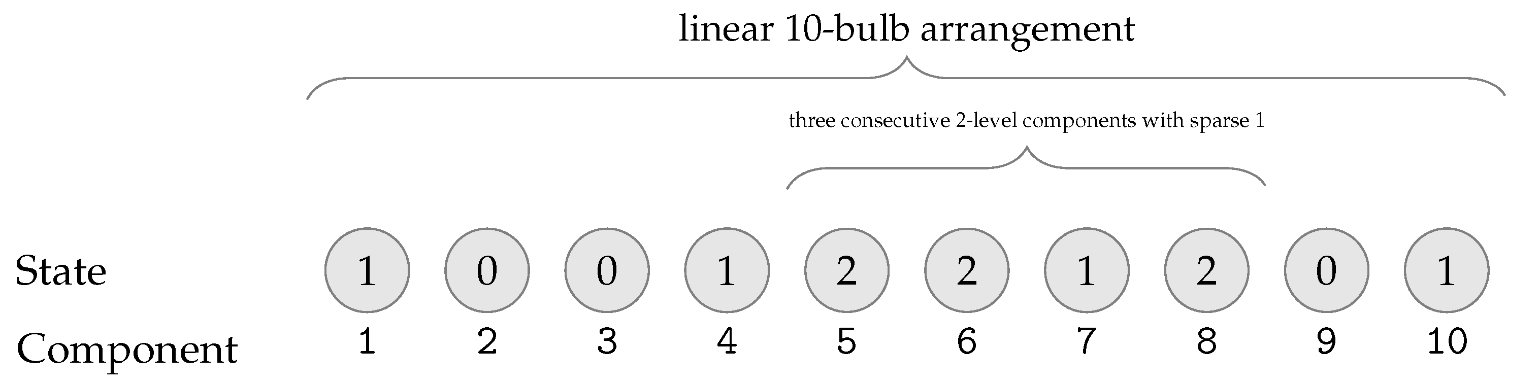
([10], Example 1). Consider a lighting system in a manufacturing workshop with ten homogeneous lamp bulbs, see Figure 1. All the bulbs are arranged linearly and each of them might be in one of three different states. State 0 is a failed state, state 1 represents a partial functioning state, and state 2 is a perfect functioning state. We want to evaluate the probability that the system can satisfy a certain requirement of brightness. According to this requirement, the system may be in one of the following states: System state 0 indicates that the lighting system does not provide enough brightness for the manufacturing system to work; system state 1 indicates that the manufacturing system can work partially by a certain amount of brightness; and system state 2 means that the lighting system provides enough brightness for the manufacturing system to work perfectly. In the lighting system, the concept of sparse d can be illustrated in terms of the coverage of light. Let $d=1$. As shown in Figure 1, components 5, 6, and 8 are in state 2 while component 7 is below state 2, then they can be regarded as 3 consecutive components in state 2 because the number of components being below state 2 between components 6 and 8 does not exceed 1. However, components 1 and 4 cannot be regarded as consecutive components in state 1 because the number of components being below state 1 between them exceeds 1.

Let us denote by $J_{k,n,d}$ the reliability ideal of a binary consecutive k-out-of-n:G system with sparse d. It is generated by all the monomials $x^{\mu }$ such that $x^{\mu }$ is the product of k consecutive variables with sparse d, i.e., $x^{\mu }=x_{i_1}\cdots x_{i_k}$ such that $i_j-i_{j-1}\le d+1$ for all $j\in \{i_2,\dots ,i_k\}$. In order to collect all such monomials, observe that:

-

$i_1$ can be any index in $\{1,\dots ,n-k+1\}$

-

For each of indices $i_j,j\in \{i_2,\dots ,i_k\}$ the gap $i_j-i_{j-1}$ must be in $\{1,\dots ,d+1\}$. Note that the sum of those $k-1$ gaps is always in $\{k-1,\dots ,n-i_1\}$.

Hence, the number of generators of $J_{k,n,d}$, i.e., the number of minimal working states of the system, is given by the following result.

Proposition 2.

Let $G\left(J_{k,n,d}\right)$ be the set of minimal generators of $J_{k,n,d}$, we have that

$$\#\left(G\left(J_{k,n,d}\right)\right)=\sum _{j=k-1}^{n-1}(n-j)\sum _{l=0}^{k-1}{(-1)}^l\left(\genfrac{}{}{0pt}{}{k-1}{l}\right)\left(\genfrac{}{}{0pt}{}{j-l(d+1)-1}{k-2}\right)$$

Proof. 

Let $C_{j,k-1,d+1}$ be the number of compositions of j in $k-1$ summands each of them in $\{1,\dots ,d+1\}$. For each index i in $\{1,\dots ,n-k+1\}$ we select k variables, starting in $x_i$, i.e., we select $k-1$ gaps, each of which is smaller than $d+1$ or equal, and the total sum cannot exceed $n-i$, being the minimal sum equal to $k-1$, since each gap is at least 1. Hence, we have that the number of generators of the ideal is

$$\sum _{i=1}^{n-k+1}\sum _{j=k-1}^{n-i}{C}_{j,k-1,d+1},$$

and a simple reorganization of the summands leads to

$$\sum _{i=1}^{n-k+1}\sum _{j=k-1}^{n-i}{C}_{j,k-1,d+1}=\sum _{j=k-1}^{n-1}(n-j)C_{j,k-1,d+1}.$$

Now, by formula E in [33] we have that

$$C_{j,k-1,d+1}=\sum _{l=0}^{k-1}{(-1)}^l\left(\genfrac{}{}{0pt}{}{k-1}{l}\right)\left(\genfrac{}{}{0pt}{}{j-l(d+1)-1}{k-2}\right),$$

and hence the result.    □

Let $G\left(J_{k,n,d}\right)=\{g_1,g_2,\dots \}$ be the set of minimal generators of $J_{k,n,d}$ and let it be sorted by the $\mathrm{lex}$ order. In order to compute the Betti numbers and Betti multidegrees of $J_{k,n,d}$, we will use Mayer–Vietoris trees and cone resolutions, cf. [18]. These are based on the iterative computation of the intersection ideals $\langle g_1,\dots ,g_{i-1}\rangle \cap \langle g_i\rangle$ where i ranges in $\left|G\right(J_{k,n,d}\left)\right|$.

Proposition 3.

Let $\mathrm{set}\left(g_i\right)$ be the set of variables in $\{x_{min\left(g_i\right)-d-1},\dots ,x_{max\left(g_i\right)}\}$ such that $x_i$ does not divide $g_i$. Then

$$\langle g_1,\dots ,g_{i-1}\rangle \cap \langle g_i\rangle =\langle x_i·g_i\mid x_i\in \mathrm{set}\left(g_i\right)\rangle +\langle g_i·g_l^{\prime }\mid g_l^{\prime }\in G\left(J_{k,min\left(g_i\right)-d-2,d}\right)\rangle$$

Proof. 

Let $\mathrm{supp}\left(g_i\right)$ be the set of variables that divide $g_i$, $max\left(g_i\right)$ be the biggest variable that divides $g_i$ and $min\left(g_i\right)$ the smallest variable that divides $g_i$.

For all $x_v\in \mathrm{set}\left(g_i\right)$, we have that $g_i\frac{x_v}{max\left(g_i\right)}=g_{i^{\prime }}\in G\left(J_{k,n,d}\right)$ with $i^{\prime }<i$ in the lex order, therefore, $x_v{g}_i\in G(\langle g_1,\dots ,g_{i-1}\rangle \cap \langle g_i\rangle )$.

If $x_v\notin \mathrm{set}\left(g_i\right)$ and $x_w\in \mathrm{supp}\left(g_i\right)$, we have that $g_i\frac{x_v}{x_w}$ either is not in $G\left(J_{k,n,d}\right)$ or it is equal to some $g_{i^{\prime }}\in G\left(J_{k,n,d}\right)$ with $i^{\prime }>i$ in the lex order. Therefore, in any case $x_v{g}_i$ it is not a minimal generator of $\langle g_1,\dots ,g_{i-1}\rangle \cap \langle g_i\rangle$.

Finally, for any $g_{i^{\prime }}\in G\left(J_{k,n,d}\right)$ such that $\mathrm{supp}\left(g_{i^{\prime }}\right)\subseteq \{1,\dots ,min\left(g_i\right)-d-2\}$ we have that $\mathrm{supp}\left(g_i\right)\cap \mathrm{supp}\left(g_{i^{\prime }}\right)=\varnothing$ and there is no $x_v\in \mathrm{set}\left(g_i\right)$ such that $x_v$ divides $g_{i^{\prime }}$ hence $\langle g_i\rangle \cap \langle g_{i^{\prime }}\rangle =\langle g_i{g}_{i^{\prime }}\rangle$, $g_i{g}_{i^{\prime }}\in G(\langle g_1,\dots ,g_{i-1}\rangle \cap \langle g_i\rangle$ and $g_i{g}_{i^{{}^{″}}}$ does not divide $g_i{g}_{i^{\prime }}$ for any other such $g_{i^{{}^{″}}}\ne g_{i^{{}^{\prime }}}$. Observe that the set given by all $g_{i^{\prime }}\in G\left(J_{k,n,d}\right)$ such that $\mathrm{supp}\left(g_{i^{\prime }}\right)\subseteq \{1,\dots ,min\left(g_i\right)-d-2\}$ is precisely $G\left(J_{k,min\left(g_i\right)-d-2,d}\right)$.    □

Theorem 1.

${\beta }_i\left(J_{k,n,d}\right)={\sum }_{x^{\mu }\in G\left(J_{k,n,d}\right)}\left(\genfrac{}{}{0pt}{}{\left|\mathrm{set}\right(x^{\mu }\left)\right|}{i}\right)+{\beta }_{i-1}\left(J_{k,min(x^{\mu }-d-2),d}\right)$

Proof. 

It is a direct consequence of Proposition 3 and the fact that

$$\mathrm{set}\left(x^{\mu }\right)\cap \mathrm{supp}\left(G\left(J_{k,min(x^{\mu }-d-2),d}\right)\right)=\varnothing .$$

   □

Observe that ${\beta }_0\left(J_{k,n,d}\right)=\#\left(G\left(J_{k,n,d}\right)\right)$ and hence the recursion in Theorem 1 is closed and it yields a procedure for the computation of the Betti numbers of $J_{k,n,d}$. From this result and applying the components’ probabilities, we obtain the reliability of the corresponding binary consecutive k-out-of-n:G system with sparse d.

We say that a binary consecutive k-out-of-n:G system with sparse d is compact if $2k\ge n-d$. For any such compact system, we have that $C_{i-d-2,k,d}=0$ for all $i=1,\dots ,n-k+1$, i.e., $J_{k,min(x^{\mu }-d-2),d}=\varnothing$ for all $x^{\mu }\in G\left(J_{k,n,d}\right)$. We therefore obtain the following consequences of Proposition 3:

Corollary 1.

Let $J_{k,n,d}$ the reliability ideal of a compact binary consecutive k-out-of-n:G system with sparse d, then $J_{k,n,d}$ has linear quotients with respect to the lex order.

Proof. 

Having linear quotients with respect an ordering of the generators means that for such ordering we have that $\langle g_1,\dots ,g_{i-1}\rangle :\langle g_i\rangle$ is generated by a set of variables $\mathrm{set}\left(g_i\right)$. This is equivalent to the fact that $\langle g_1,\dots ,g_{i-1}\rangle \cap \langle g_i\rangle =\langle x_i·g_i\mid x_i\in \mathrm{set}\left(g_i\right)\rangle$. Proposition 3 and the fact that for compact systems $J_{k,min(x^{\mu }-d-2),d}=\varnothing$ for all $x^{\mu }\in G\left(J_{k,n,d}\right)$ yield the result.    □

Corollary 2.

Let $J_{k,n,d}$ be a compact binary consecutive k-out-of-n:G system with sparse d, then

$${\beta }_i\left(J_{k,n,d}\right))=\sum _{x^{\mu }\in G\left(J_{k,n,d}\right)}\left(\genfrac{}{}{0pt}{}{\left|\mathrm{set}\right(x^{\mu }\left)\right|}{i}\right).$$

Observe that a binary consecutive k-out-n ordinary system, i.e., $d=0$, is compact if and only if $k\ge n/2$

Example 8.

Let $n=9$, $k=3$, $d=2$. The corresponding consecutive k-out-of-n with sparse d system is not compact. The list of minimal monomial generators of $J_{k,n,d}$ has 45 generators and is given by the monomials $x^{\mu }=x_a{x}_b{x}_c$ for all triples $abc$ in the following set (given in $\le x$ order)

$$\begin{array}{cc}\hfill & 123,124,125,134,135,136,145,146,147,\hfill \\ \hfill & 234,235,236,245,246,247,256,257,258,\hfill \\ \hfill & 345,346,347,356,357,358,367,368,369,\hfill \\ \hfill & 456,457,458,467,468,469,478,479,\hfill \\ \hfill & 567,568,569,578,579,589,\hfill \\ \hfill & 678,679,689,\hfill \\ \hfill & 789.\hfill \end{array}$$

Example 9.

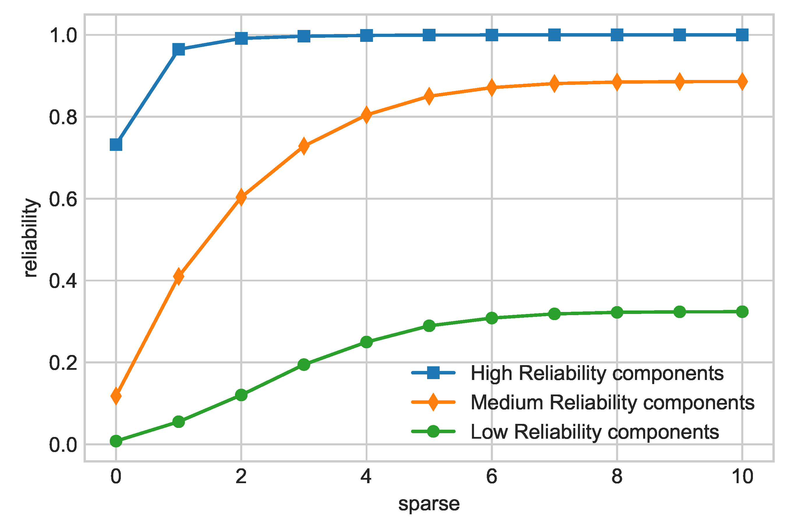
Let $n=15$, $k=5$ and let d range from 0 to 10. When $d=0$, we have the usual consecutive 5-out-of-15 system, and as d increases we tend towards the traditional k-out-of-n system, which occurs when $d>n-k$. Let us assign working probabilities to the components in three ways: First consider highly reliable components, i.e., $p_{i,1}=0.8$ if i is odd and $p_{i,1}=0.7$ if i is even; second, consider medium reliable components, i.e., $p_{i,1}=0.5$ if i is odd and $p_{i,1}=0.4$ if i is even and finally consider components with low reliability, $p_{i,1}=0.3$ if i is odd and $p_{i,1}=0.2$ if i is even. Figure 2 shows the behaviour of the reliability of these three kinds of systems as the sparse d varies.

For the multi-state case, the situation is similar to multi-state consecutive k-out-of-n systems. Gao, Cui and Chen define multi-state consecutive k-out-of-n:G system with sparse d in [10] in the following way.

Definition 2.

A system with n components is called a generalized multi-state consecutive k-out-of-n:G system with sparse d if $\Phi \left(X\right)\ge j,(1\le j\le M)$ whenever there exists an integer value $l,(j\le l\le M)$ such that at least consecutive $k_l$ components are in state l or above with sparse d.

As in MS consecutive k-out-of-n systems, we consider increasing, decreasing and constant generalized MS consecutive k-out-of-n:G system with sparse d systems depending on the sequence of $k_j$ for the different levels j.

Applying the same reasoning as in Section 3, we define $J_{k,n,d,j}$ as the ideal generated by the generators of $J_{k,n,d}$ each raised to the j-th power. We then define the ideal of a multi-state consecutive k-out-of-n:G system with sparse d as

$${\overline{J}}_{k,n,d,j}=\bigcap _{j^{\prime }\le j}{J}_{k_{j^{\prime }},n,j^{\prime },d}$$

Example 10.

In the system in Example 7, see [10], to reach system state 1, it is required that at least consecutive 3-out-of-10 light bulbs should be in state 1 or above with sparse 1. To reach state 2, i.e., to meet the demand of enough brightness, at least consecutive 5-out-of-10 light bulbs should be in state 2 or above with sparse 1. Therefore, we can model the mentioned example as an increasing MS consecutive $(k_1,k_2)$-out-of-10:G system model with sparse 1, where $k_1=3$ and $k_2=5$. Using Proposition 2, we have that the number of generators of ${\overline{J}}_{3,10,1,1}$ is 28 and the number of generators of ${\overline{J}}_{5,10,1,2}$ is 64. In both cases, the computation of the Betti numbers and j-reliabilities (and bounds) of this system is computed in less than one second by our algorithms.

Example 11.

Let $n=15$ and $k_1=2,k_2=5,k_3=7,k_4=9$. We consider multi-state consecutive k-out-of-n:G systems with sparse d such that the systems have 4 different working levels. Take $d=3,5,7$. The components are independent but non-identical. The probabilities of each component being in the different sates are given as follows: $p_{i,0}=0.1$, $p_{i,1}=0.15$, $p_{i,2}=0.2$, $p_{i,3}=0.25$ and $p_{i,4}=0.3$ if i is odd, and $p_{i,0}=0.05$, $p_{i,1}=0.15$, $p_{i,2}=0.2$, $p_{i,3}=0.25$ and $p_{i,4}=0.35$ if i is even. The number of generators for the corresponding ideals and the reliabilities and computation times for each of these systems are given in

Table 3. Number of generators of the ideals of several multi-state consecutive k-out-of-n:G systems with sparse d and times to compute their reliability.

n	k	d	j	num.gens.	Reliability	Time (s)
15	2	3	1	50	0.9999996	0.004018
15	5	3	2	1281	0.99801	0.152161
15	7	3	3	4470	0.785976	2.04139
15	9	3	4	4565	0.0233618	4.49723
15	2	5	1	69	0.9999996	0.003935
15	5	5	2	2499	0.999723	0.343454
15	7	5	3	6219	0.857467	4.90422
15	9	5	4	4997	0.0250292	5.43077
15	2	7	1	84	0.9999998	0.00347
15	5	7	2	2919	0.999942	0.480944
15	7	7	3	6429	0.863406	5.61369
15	9	7	4	5005	0.0250567	5.40056

. The column reliability indicates the probability that the system is at level j or greater.

Multi-State Consecutive k-out-of-n:G Systems with Sparse d and Maximum Total Gap m

In multi-state consecutive systems, Huan et al. [34] consider the situation in which a system may fail when a number of consecutive failures takes place or when a total number of failures (maybe not consecutive) occur, see also [35]. This situation can be applied to multi-state consecutive k-out-of-n:G systems with sparse d and therefore extend this model to a wider range of situations. We consider as before that two components whose states are l or above are consecutive if all the components between them are below state l and the number of such components is at most d, in addition, we say that k components $c_1,\dots ,c_k$ are consecutive only if they are pairwise consecutive in this sense and the total number of components in state l or below between $c_1$ and $c_k$ is at most m. With this restriction we give the following definition:

Definition 3.

A system with n components is called a generalized MS consecutive k-out-of-n:G system with sparse d and maximum total gap m if $\Phi \left(X\right)\ge j$$(1\ge j\ge M)$ whenever there exists an integer value l, $(j\ge l\ge M)$ such that at least consecutive $k_l$ components are in state l or above with sparse d and the number of components below state l within them is at most m.

Let us denote by $J_{k,n,d,m}^{\prime }$ the ideal of a binary consecutive k-out-of-n:G system with sparse d and maximum total gap m. Following the proof of Proposition 2, we have that the number of generators of $J_{k,n,d,m}^{\prime }$ is given by a truncation of the sum in the number of generators of $J_{k,n,d}$.

Proposition 4.

Let $G\left(J_{k,n,d,m}^{\prime }\right)$ be the set of minimal generators of $J_{k,n,d,m}^{\prime }$, we have that

$$\#\left(G\left(J_{k,n,d,m}^{\prime }\right)\right)=\sum _{j=k-1}^m(n-j)\sum _{l=0}^{k-1}{(-1)}^l\left(\genfrac{}{}{0pt}{}{k-1}{l}\right)\left(\genfrac{}{}{0pt}{}{j-l(d+1)-1}{k-2}\right)$$

Observe that if $m\ge n-1$ then the system is a consecutive k-out-of-n:G system with sparse d.

Example 12.

Consider the system in Example 8. We have $n=9$, $k=3$, $d=2$, and set $m=3$. Now, components 1, 4 and 7 are consecutive with sparse 2 but the total number of failed components between 1 and 7 is four, hence, this would be a failure state for a consecutive 3-out-of-9:G system with sparse 2 and maximum total gap 3. For such a system, the list of minimal monomial generators of its reliability ideal $J_{k,n,d,m}^{\prime }$ has 42 elements and is given by the monomials $x^{\mu }=x_a{x}_b{x}_c$ for all triples $abc$ in the following set (given in lex order)

$$\begin{array}{cc}\hfill & 123,124,125,134,135,136,145,146,\hfill \\ \hfill & 234,235,236,245,246,247,256,257,\hfill \\ \hfill & 345,346,347,356,357,358,367,368,\hfill \\ \hfill & 456,457,458,467,468,469,478,479,\hfill \\ \hfill & 567,568,569,578,579,589,\hfill \\ \hfill & 678,679,689,\hfill \\ \hfill & 789.\hfill \end{array}$$

Example 13.

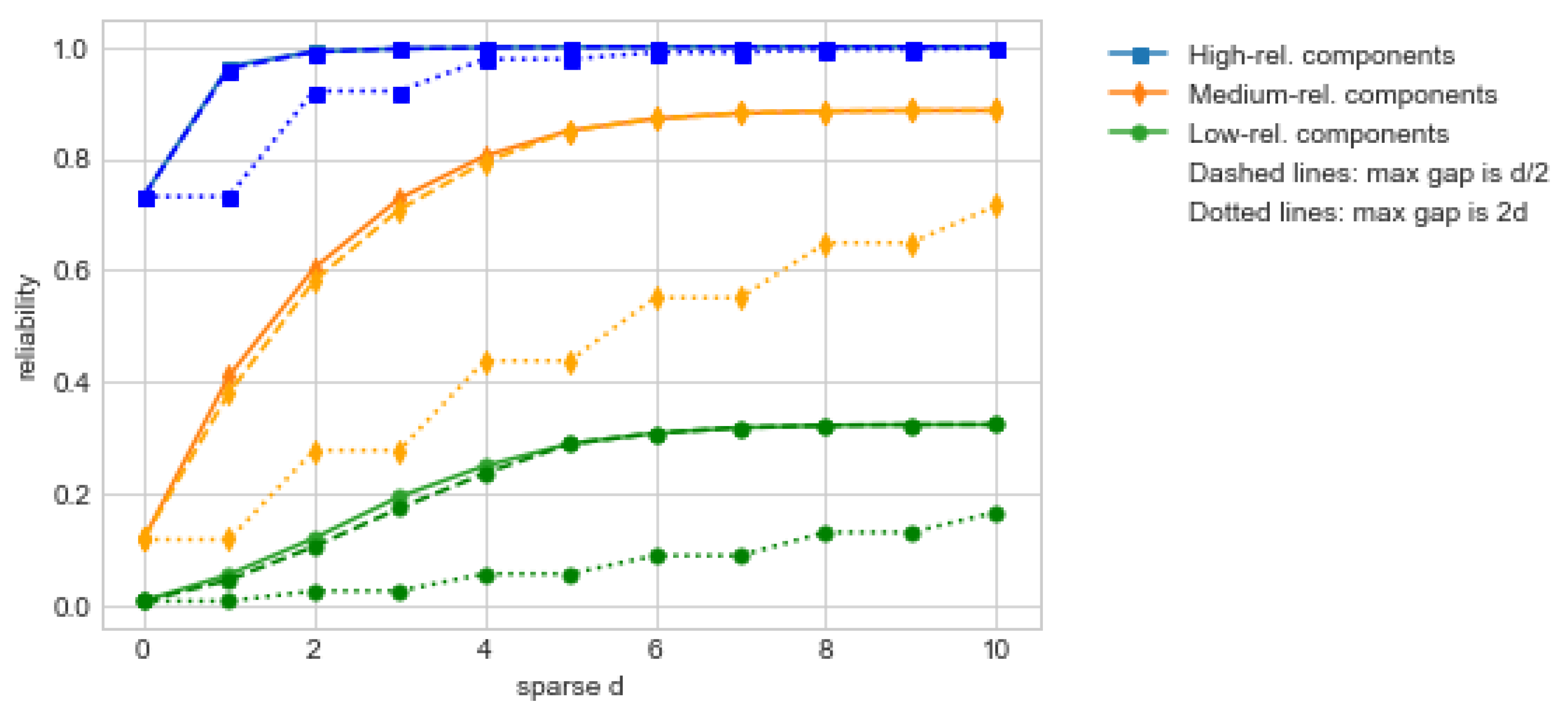
Figure 3 shows the effect of setting the maximum gap at half the sparse and twice the sparse in the systems of Example 9. In both cases, the reliability of the system is reduced as expected, by a small amount in case the gap is half the sparse, and by a larger amount in case the maximum allowed gap doubles the sparse of the system.

5. Weighted Multi-State $k$-out-of-$n$ Systems

The traditional binary k-out-of-n system model was extended by Wu and Chen [36] to weightedk-out-of-n systems. In a binary weighted k-out-of-n:G system, component i has a weight $w_i$. The weight of each component represents the utility of the component, i.e., its contribution to the actual performance of the system. The system works if and only if the total weight of the working components is at least k, a pre-specified value. Observe that k may be larger than n. The multi-state version of weighted k-out-of-n systems was introduced by Li and Zuo in [9] where the authors define two variants of these systems.

Definition 4

(Weighted multi-state k-out-of-n system, model I). In a system with n components, each component and system may be in $M+1$ possible states, $\{0,\dots ,M\}$. Component i $(1\le i\le n)$, when in state j $(0\le j\le M)$, has a utility value of $w_{i,j}$. The system is in state j or above if the total utility of all components is greater than or equal to $k_j$, a pre-specified value. Let Φ be the structure function of the system representing the state of the system and W the total utility of all components. Then, this definition means $\mathrm{Pr}\{\Phi \ge j\}=\mathrm{Pr}\{W\ge k_j\}$. Since state 0 is the worst state of the system, we have $\mathrm{Pr}\{\Phi \ge 0\}=1$.

For the second definition, we consider only the contribution of those components in state j or above.

Definition 5

(Weighted multi-state k-out-of-n system, model II). The system is in state j or above if the sum of the weights of the components whose states are in state j or above is greater than or equal to $k_j$. Let Φ be the structure function of the system and $W_j$ be the sum of the utilities of the components whose states are j or above. We then have $\mathrm{Pr}\{\Phi \ge j\}=\mathrm{Pr}\{W_j\ge k_j\}$.

Since the structure functions of these kinds of systems depend strongly on the individual contributions or weights of each of the variables, the methods for computing its reliability are of an enumerative nature. Li and Zuo evaluate in [9] two such methods: a recursive one [36,37] and the Universal Generating Function Method (UGF) [2,3,11]. The analysis in [9] shows that, in general, the recursive approach is more effective than the UGF method for both models I and II. A key issue in the algorithmic evaluation of these systems’ reliability is the efficiency in enumerating the working states for each level.

For any monomial ideal $I\subseteq \mathbf{k}[x_1,\dots ,x_n]$, a quotient basis is a basis as a $\mathbf{k}$-vector space of the quotient ring $R/I$. It amounts to a way of enumerating all the monomials that are not in I. In our case, considering $I=\langle x_1^{M+1},\dots ,x_n^{M+1}\rangle$ we have that the ${(M+1)}^n$ monomials not in I correspond to all possible states of the system’s components. In order to obtain the reliability of the system, we proceed state by state and add the probabilities of the states whose weight is above $k_j$ for each j. This methodology might theoretically be less efficient than the recursive or the UGF approach, but a good implementation of the enumeration step can compensate this. This is indeed the case with the CoCoALib function QuotientBasis which is an efficient implementation of the enumeration of the elements in the $\mathbf{k}$-basis of $R/I$ for any ideal I.

Table 4. $n=5$, $k_1=200$, average of ten runs.

M	TS	WS	RS	TS-Time (s)	WS-Time (s)	RS-Time (s)
3	243	0	0	0.006094	0.006162	0
4	1024	0	0	0.007245	0.007462	0
5	3125	3	1	0.008029	0.008848	0.008869
6	7776	44	5	0.009567	0.011285	0.011382
7	16,807	410	26	0.01666	0.018772	0.019281
8	32,768	5398	293	0.028787	0.36573	0.044584
9	59,049	16,204	179	0.091856	0.101756	0.113455
10	100,000	32,768	390	0.150313	0.166822	0.193492
11	161,051	76,570	373	0.3017117	0.351811	0.413162
12	248,832	121,508	326	0.427333	0.482606	0.583472

and

Table 5. $M=5$, $k_1=200$, average of ten runs.

n	TS	WS	RS	TS-Time (s)	WS-Time (s)	RS-Time (s)
3	125	0	0	0.00592	0.005949	0
4	625	0	0	0.006535	0.006662	0
5	3125	0	0	0.006134	0.006803	0
6	15,625	20	7	0.15506	0.017679	0.017708
7	78,125	3873	302	0.01859	0.036595	0.04394
8	390,625	46,945	2106	0.11527	0.120179	0.214819
9	1,953,125	224,695	3561	0.155288	0.422814	0.889363
10	9,765,625	1,662,628	24,131	0.738989	2.4139	18.5923
11	48,828,125	10,022,724	31,389	3.812	12.1875	64.2796

show the results of some computer experiments in systems of the same kind as those in the experiments in [9]. In Table 4, we set $n=5$ and take M from 3 to 12. Each component’s weight is a random integer number in the range $[1,14]$ and probabilities are randomly assigned. In Table 5, the weights and probabilities are assigned in the same way but we keep M constant and equal to 5 while n varies from 3 to 11. In both cases, we set $k_1=200$. In the tables, column $TS$ indicates the total number of possible states of the system, column $WS$ indicates the number of j-working states and column $RS$ indicates the size of the set of minimal working states. The number of working states was obtained by exhaustive search on the possible states of the systems, and the number of minimal states was obtained by the minimization algorithm implemented in CoCoALib. For each of these numbers, there is a column indicating the time used for its computation by the C++ class described in [28]. Observe that [9] shows the results of another set of examples in which the weights assigned to the variables are floating point numbers in the range $[20,50]$ this affects the performance of the UGF method, since there are less like terms to cancel, but it does not affect the recursive method. It does not affect the performance of our approach either, since our method is based on the efficiency of the algebraic approach to enumeration of all working states. Observe that in these tables, the time for the computation of the reliability of the system is that in the WS-time column. The tables show computations Model I systems, the algorithms and results are essentially equivalent for Model II.

The described procedure computes the exact reliability of weighted k-out-of-n systems. In case one is interested in the algebraic bounds as obtained in the previous sections, we need to consider the ideal generated by the monomials corresponding to working states of the system. In this case, the first step is to obtain the set of minimal working states, or equivalently the minimal set of generators of the corresponding ideal. The complexity of this procedure, starting with the complete set of working states is $O\left(r^2\right)$ where r is the total number of working states of the system. It is, therefore, an impractical procedure for large systems. In Table 4 and Table 5, the time for computing the minimal generating set of the j-ideal, i.e., the minimal set of working states is given under column RS-time. The size of these sets is under column $RS$ and one can see that these sizes are significantly smaller than that of the set of working states, hence, it would be worth investigating efficient ways of obtaining these sets directly. This would imply a drastic reduction of the computing time of the reliability and bounds for weighted multi-state k-out-of-n systems.

6. Conclusions and Further Work

We have presented in this work an algebraic approach to the reliability analysis of several important multi-state systems, to which it had not been applied before, namely, variants of the classical multi-state k-out-of-n model. This approach not only provides insight on the structure of the system and it features, such as the number of minimal working states, e.g., for multi-state consecutive k-out-of-n:G systems with sparse d systems, but also produces efficient algorithms for computing the reliability of the systems and bounds for it. The analyses performed in this work demonstrate the versatility of the algebraic approach to system reliability and fosters further analysis of other important systems, like networks. Further work includes also to study the relations and possible combination with other related methods like the Universal Generating Function method, Binary Decision Trees and others.

References

- Kuo, W.; Zuo, M.Z. Optimal Reliability Modelling; Wiley and Sons: Hoboken, NJ, USA, 2002. [Google Scholar]
- Lisnianski, A.; Frenkel, I.; Ding, Y. Multi-State System Reliability Analysis and Optimization for Engineers and Industrial Managers; Springer: Berlin/Heidelberg, Germany, 2010. [Google Scholar]
- Lisnianski, A.; Levitin, G. Multi-State System Reliability; World Scientific: Singapore, 2003. [Google Scholar]
- Natvig, B. Multistate Systems Reliability Theory with Applications; Wiley and Sons: Hoboken, NJ, USA, 2011. [Google Scholar]
- Yingkui, G.; Jing, L. Multi-state system reliability: An new and systematic review. Procedia Eng. 2012, 29, 531–536. [Google Scholar] [CrossRef] [Green Version]
- Huang, J.; Zuo, M.J.; Wu, Y. Generalized Multi-state k-Out Systems. IEEE Trans. Reliab. 2000, 49, 105–111. [Google Scholar] [CrossRef]
- Mo, Y.; Liudong, X.; Amari, S.V.; Dugan, J.B. Efficient analysis of multi-state k-Out Systems. Reliab. Eng. Syst. Saf. 2015, 133, 95–105. [Google Scholar] [CrossRef]
- Huang, J.; Zuo, M.J.; Fang, Z.D. Multi-state consecutive k-Out Systems. IIE Trans. 2003, 35, 527–534. [Google Scholar] [CrossRef]
- Li, W.; Zuo, J. Reliability evaluation of multi-state weighted k-Out Systems. Reliab. Eng. Syst. Saf. 2008, 93, 160–167. [Google Scholar] [CrossRef]
- Gao, H.; Cui, L.; Chen, J. Reliability Modeling for Sparsely Connected Homogeneous Multistate consecutive k-Out Systems. IEEE Trans. Syst. Man Cybern. Syst. 2021, 51, 1844–1854. [Google Scholar] [CrossRef]
- Ushakov, I. Optimal standby problem and a universal generating function. Sov. J. Comput. Sys. Sci. 1987, 25, 61–73. [Google Scholar]
- Giglio, B.; Wynn, H.P. Monomial ideals and the Scarf complex for coherent systems in reliability theory. Ann. Stat. 2004, 32, 1289–1311. [Google Scholar] [CrossRef] [Green Version]
- Sáenz-de-Cabezón, E.; Wynn, H.P. Betti numbers and minimal free resolutions for multi-state system reliability bounds. J. Symb. Comput. 2009, 44, 1311–1325. [Google Scholar] [CrossRef] [Green Version]
- Sáenz-de-Cabezón, E.; Wynn, H.P. Mincut ideals of two-terminal networks. Appl. Algebra Eng. Commun. Comput. 2010, 21, 443–457. [Google Scholar] [CrossRef]
- Sáenz-de-Cabezón, E.; Wynn, H.P. Hilbert functions for design in reliability. IEEE Trans. Reliab. 2015, 64, 83–93. [Google Scholar] [CrossRef]
- Sáenz-de-Cabezón, E.; Wynn, H.P. Computational algebraic algorithms for the reliability of generalized k-out-of-n and related systems. Math. Comput. Simul. 2011, 82, 68–78. [Google Scholar] [CrossRef]
- Pascual-Ortigosa, P.; Sáenz-de-Cabezón, E.; Wynn, H. Algebraic reliability of multi-state k-out-of-n systems. Probab. Eng. Inf. Sci. 2020, in press. [Google Scholar] [CrossRef]
- Sáenz-de-Cabezón, E. Multigraded Betti numbers without computing minimal free resolutions. Appl. Alg. Eng. Commun. Comput. 2009, 20, 481–495. [Google Scholar] [CrossRef]
- El-Neweihi, E.; Proschan, F.; Sethurman, J. Multi-state coherent systems. J. Appl. Probab. 1978, 15, 675–688. [Google Scholar] [CrossRef]
- Barlow, R.E.; Proschan, F. Statistical Theory of Reliability and Life Testing: Probability Models; Holt, Rinehart and Winston: Austin, TX, USA, 1975. [Google Scholar]
- Belaloui, S.; Ksir, B. Reliability of a multistate consecutive k-Out System. Int. J. Rel. Qual. Saf. Eng. 2007, 14, 361–377. [Google Scholar] [CrossRef]
- Yamamoto, H.; Zuo, M.J.; Akiba, T.; Tian, Z.G. Recursive formulas for the reliability of multistate consecutive k-Out Systems. IEEE Trans. Reliab. 2006, 55, 98–104. [Google Scholar] [CrossRef]
- Zhao, X.; Xu, Y.; Liu, F.Y. State distributions of multistate consecutive k Systems. IEEE Trans. Reliab. 2012, 61, 274–281. [Google Scholar] [CrossRef]
- Fu, J.C. Reliability of consecutive k-Out F Syst. (k-1) Markov Dependence. IEEE Trans. Reliab. 1986, 35, 602–606. [Google Scholar] [CrossRef]
- Koutras, M.V. On a Markov Chain Approach for the Study of Reliability Structures. J. Appl. Probab. 1996, 33, 357–367. [Google Scholar] [CrossRef]
- Yi, H.; Cui, L.; Gao, H. Reliabilities of Some Multistate consecutive k Systems. IEEE Trans. Reliab. 2020, 69, 414–429. [Google Scholar] [CrossRef]
- Dohmen, K. Improved Bonferroni Inequalities via Abstract Tubes; Springer: Berlin/Heidelberg, Germany, 2003. [Google Scholar]
- Bigatti, A.; Pascual-Ortigosa, P.; Sáenz-de-Cabezón, E. A C++ class for multi-state algebraic reliability computations. Reliab. Eng. Syst. Saf. 2021, 27, 107751. [Google Scholar] [CrossRef]
- Butler, D.A. Bounding the reliability of multistate systems. Oper. Res. 1982, 30, 530–544. [Google Scholar] [CrossRef]
- Funnemark, E.; Natvig, B. Bounds for the availabilities in a fixed time interval for multistate monotone systems. Adv. Appl. Prob. 1985, 17, 638–665. [Google Scholar] [CrossRef]
- Gåsemyr, J.; Natvig, B. Improved availability bounds for binary and multistate monotone systems with independent component processes. J. Appl. Probab. 2017, 54, 750–762. [Google Scholar] [CrossRef] [Green Version]
- Zhao, X.; Cui, L.R.; Kuo, W. Reliability for sparsely connected consecutive k systems. IEEE Trans. Reliab. 2007, 56, 516–524. [Google Scholar] [CrossRef]
- Abramson, M. Restricted combinations and compositions. Fibonacci Q. 1976, 14, 439–456. [Google Scholar]
- Huan, Y.; Jun, Y.; Rui, P.; Yu, Z. Reliability evaluation of linear multi-state consecutively-connected systems constrained by m Consecutive n Total Gaps. Reliab. Eng. Syst. Saf. 2016, 150, 35–43. [Google Scholar]
- Levitin, G.; Xing, L.; Dai, Y. Linear multistate consecutively-connected systems subject to a constrained number of gaps. Reliab. Eng. Syst. Saf. 2015, 133, 246–252. [Google Scholar] [CrossRef]
- Wu, J.S.; Chen, R.J. An algorithm for computing the reliability of a weighted-k-out-of-n system. IEEE Trans. Reliab. 1994, R-43, 327–328. [Google Scholar]
- Higashiyama, Y. A factored reliability formula for weighted-k-Out System. Asia-Pac. J. Oper. Res. 2001, 18, 61–66. [Google Scholar]
Figure 1.
Lighting system: bulb linear arrangement in Example 7.
Figure 2.
System reliability for consecutive 5-out-of-15 systems with sparse . Low, medium and high reliability components.
Figure 3.
System reliability for consecutive 5-out-of-15 systems with sparse and maximum gap set as or . Systems with low, medium and high reliability components.