Stability Analysis of Pseudo-Almost Periodic Solution for a Class of Cellular Neural Network with D Operator and Time-Varying Delays

Abstract

Cellular neural networks with D operator and time-varying delays are found to be effective in demonstrating complex dynamic behaviors. The stability analysis of the pseudo-almost periodic solution for a novel neural network of this kind is considered in this work. A generalized class neural networks model, combining cellular neural networks and the shunting inhibitory neural networks with D operator and time-varying delays is constructed. Based on the fixed-point theory and the exponential dichotomy of linear equations, the existence and uniqueness of pseudo-almost periodic solutions are investigated. Through a suitable variable transformation, the globally exponentially stable sufficient condition of the cellular neural network is examined. Compared with previous studies on the stability of periodic solutions, the global exponential stability analysis for this work avoids constructing the complex Lyapunov functional. Therefore, the stability criteria of the pseudo-almost periodic solution for cellular neural networks in this paper are more precise and less conservative. Finally, an example is presented to illustrate the feasibility and effectiveness of our obtained theoretical results.

1. Introduction

In recent years, the cellular neural networks (CNN), first proposed by Chua and Yang [1,2], have received significant attention because of their wide applications in science and engineering technology fields. Extensive research has been conducted on CNN in the past few decades, and one of the primary problems in designing CNN is to deal with the dynamic curves of existing solutions. Regarding the existence, uniqueness, and stability of the periodic, almost periodic solutions of neural networks, there have been many results in the fields of classification, signal processing [3], associative memory [4,5], optimal control [6], and filter problem [7,8,9]. The state estimation problem of delayed static neural networks has been considered by Wang and Xia et al. [10]. Donkers et al. showed stability analysis results of networked control systems employing a switched linear systems approach [11]. Liang and Wang et al. [12], mainly examined the robust synchronization issue for two-dimension discrete-time coupled dynamical neural networks. Due to the limited bandwidth speed and the constraints of physical property for circuit equipment, information propagation inevitably give birth to the emergence of time delays, meanwhile arising other problems of the CNN. The appearance of time lags usually causes turbulence, instability, and chaos [13,14]. The stability of discrete-time systems with time-varying delays via a novel summation inequality was discussed in [15,16]. For the reason that information transmission between neurons has time delays behavior, the neural network model with delay described by the time delays functional differential equation has been widely examined and implemented in various fields.

Due to similarity to the circuit system’s connection, CNN is a practical and feasible alternative to the circuit system simulation [17]. Many scholars realized the vital of neural networks and introduced novel research methods to work with their dynamic behavior [18,19]. Subsequently, some scholars also proposed several different types of CNN models and discussed the dynamic characteristics of solution curves [20,21]. In 2018, hierarchical type stability criteria for delayed neural networks via canonical Bessel–Legendre inequalities had been demonstrated [22]. In particular, shunt suppression of artificial CNN has been widely used in various research fields such as pattern recognition [23], image processing [24], and combination optimization [25]. The dynamic characteristics of neural networks, such as the existence, uniqueness, and global asymptotic stability of the equilibrium point and periodic solution for time-delay CNN play a crucial role. However, most of the existing results on the dynamic behavior of CNN focus on stability or periodicity. Fewer have been done on the existence of periodic solutions or almost periodic solutions for Cohen–Grossberg neural networks with delays [26,27].

Many motion processes in the present world are approximate to periodic instead of strictly periodicity. Conventionally, to reduce computing tasks’ burden, the complex system is usually idealized as a periodic. However, the system may not have periodicity for various CNN systems, even though all its parameters are periodic due to the uncertainty of the system’s parameters’ periodicity. Hence, the complex system may have no periodic solution curves. Danish mathematicians Bohr [28] first proposed the concept of almost periodicity, which is a significant generalization for practical application. Following the work proposed by Bohr, some scholars have been put forward many different techniques to expand the research of almost periodic solutions of complex systems [29,30]. Similarly, the concept of pseudo-almost periodicity was proposed by Zhang [31] in 1992, and it was further extended from the natural almost periodic to the pseudo-almost periodic in the Bohr sense.

Including many commonly used forms that may exist, the dynamic behavior of pseudo-almost periodicity is more extensive and approximate to the actual [32]. Therefore, the described neural network characteristic has a high degree of complexity and importance significance [33]. In CNN systems, the process of information transmission and mutual reaction between neurons is exceptionally complicated, and various phenomena such as disturbance, instability, bifurcation, and chaos may occur [34]. Therefore, it is of both theoretical and practical vital to examine the dynamic behavior of CNN systems pseudo-almost periodicity. There is relatively tiny related literature on pseudo-almost periodic research so far. For example, Liu [35] studied the pseudo-almost periodic solutions for neutral-type CNN with continuously distributed leakage delays; and others investigated the pseudo-almost periodic solutions for a Lasota–Wazewska model with an oscillating death rate [36]. As far as we know, there is still a massive gap in the investigation of the pseudo-almost periodicity, insufficient work was done on the existence and stability of pseudo-almost periodic solutions on neural networks with proportional delays [37]. Therefore, based on the previous examined, further exploration of the pseudo-almost periodic solution is one of the targets for this work. The main contributions of this paper are as follows: (1) This work not only considered the D operator systems but also investigated the effects of time-delays on dynamical complex network systems. (2) The approach we utilized was completely different previous. (3) The stability criteria of the pseudo-almost periodic solution in this paper are more precise and less conservative. (4) Compared with previous studies on the stability criteria, analyzing the globally exponentially stable avoids constructing the complex Lyapunov functional.

By employing innovative fixed-point theory and exponential dichotomy methods, we derived the pseudo-almost periodic solutions stability issue, which is entirely different from earlier work. The obtained results in this paper are novel, meanwhile promoting and supplement some of the previous research work. The r-neighborhood of a cell $x_{ij}$ defines as follows:

$$N_r^0(i,j)=\{x_{pq}|d_{ij,pq}=\sqrt{|p-i{|}^2+|q-j{|}^2}\le \frac{r}{2},1\le p\le m,1\le q\le n\},$$

where $r\ge 2$ is a positive integer number. Since each cell of CNN is only connected to its neighboring areas, those cells that are not directly connected may be affected by continuous-time propagation effects and indirectly affect each other. Furthermore, due to the neural network’s increasing distance, the influence between different neurons in CNN is correspondingly weakened.

Several previous works are the motivation for us to propose the new r-neighborhood $N_r^0(i,j)$, we examined the novel types of cellular neural networks with D operator and time-varying delays as follows:

$$\begin{array}{l}[x_{ij}(t)-p_{ij}(t)x_{ij}(t-{\delta }_{ij}(t))]\prime \\ =-a_{ij}(t)x_{ij}(t)+{\displaystyle \sum _{i=1}^m}{\displaystyle \sum _{j=1}^n{b}_{ij}(t)}{f}_{ij}(t,x_{i-1j}(t),x_{ij-1}(t),x_{ij+1}(t),x_{i+1j}(t))\\ \stackrel{}{{\displaystyle }}+{\displaystyle \sum _{i=1}^m}{\displaystyle \sum _{j=1}^n{c}_{ij}(t)}{g}_{ij}(t,x_{i-1j}^{\tau }(t),x_{ij-1}^{\tau }(t),x_{ij+1}^{\tau }(t),x_{i+1j}^{\tau }(t))+L_{ij}(t),\end{array}$$

(1)

where $x_{ij}^{\tau }(t)=x_{ij}(t-{\tau }_{ij}(t)),1\le i\le m,1\le j\le n.$ $x_{ij}(t)$ corresponds to the state of the $ij-th$ cell (at the (i, j) position of the lattice) at time t, $a_{ij}(t)>0$ represents the rates with which the $ij-th$ cell will reset its potential to the resting state in isolation when disconnected from the networks and external inputs at time t; $f_{ij}(\cdot )$, $g_{ij}(\cdot )$ denote the activation functions of signal transmission. $p_{ij}(t)$, $b_{ij}(t)$, $c_{ij}(t)$ denote the connection weights at time t, ${\delta }_{ij}(t)\ge 0,{\tau }_{ij}(t)\ge 0$ corresponding to the transmission delays, and $L_{ij}(t)$ are the external inputs on the $ij-th$ cell at time t.

The initial conditions of the system (1) are assumed to be

$$x_{{}_{ij}}^{\prime }(s)={\varphi }_{ij}(s),\stackrel{}{{\displaystyle }}s\in [-\tau ,0],1\le i\le m,1\le j\le n,$$

(2)

where ${\varphi }_{ij}(s)$ is a continuous function,

$$\tau ={\max }_{1\le i\le m,1\le j\le n}{\sup }_{t\in ℝ}\{|{\delta }_{ij}(t)|,|x_{i-1j}(t)|,|x_{ij-1}(t)|,|x_{ij+1}(t)|,|x_{i+1j}(t)|\}.$$

The paper is organized as follows. In Section 2, we will introduce some definitions and lemmas, which will be used to obtain our results. In Section 3, we state and demonstrate the existence and global exponential stability of the pseudo-almost periodic solution. In Section 4, an example illustrates the feasibility and effectiveness of obtained theoretical results. In Section 5, a brief conclusion is given.

2. Preliminaries

In this section, we recall briefly some basic definitions and properties of pseudo-almost periodic functions and the exponential dichotomy.

Definition 1.

Let$u(\cdot )\in BC(ℝ,{ℝ}^n).$$u(\cdot )$is said to be (Bohr) almost periodic on${ℝ}^n$, if for any$\epsilon >0$, the set

$$T(u,\epsilon )=\{\delta :\parallel u(t+\delta )-u(t){\parallel }_{\infty }<\epsilon ,\forall t\in ℝ\},$$

is relatively dense, i.e., for any$\epsilon >0$, it is possible to find a real number$l=l(\epsilon )>0$with the property that for any interval with length$l(\epsilon )$, there exists a number$\delta =\delta (\epsilon )$in this interval such that

$$\parallel u(t+\delta )-u(t){\parallel }_{\infty }<\epsilon ,\stackrel{}{{\displaystyle }}\forall t\in ℝ$$

Definition 2.

A function$F\in BC(ℝ\times {ℝ}^n,{ℝ}^n)$is called (Bohr) almost periodic in$t\in ℝ$uniformly in$x\in K$, where$K$ is any bounded compact subset of${ℝ}^n$, that is, if for each$\epsilon >0$, there exists$l(\epsilon )>0$ such that every interval of length$l(\epsilon )>0$contains a number$\tau$with the following property

$$\underset{t\in ℝ}{\sup }\parallel F(t+\tau ,x)-F(t,x)\parallel <\epsilon .$$

We denote by $AP(t\in ℝ\times {ℝ}^n,{ℝ}^n)$ the set of the almost periodic functions from $ℝ\times {ℝ}^n$ to ${ℝ}^n$. Additionally, we define a class function as follows:

$$PA{P}_0(ℝ\times {ℝ}^n;{ℝ}^n)=\{f\in BC(ℝ\times {ℝ}^n;{ℝ}^n)|\underset{T\to \infty }{\lim }\frac{1}{2T}{\displaystyle {\int }_{-T}^T\parallel f(t,x)\parallel dt=0,\forall x\in ℝ}\}$$

which is a closed subspace of $BC(ℝ\times {ℝ}^n;{ℝ}^n)$.

Definition 3.

A continuous function$f\in BC(ℝ\times {ℝ}^n;{ℝ}^n)$is called pseudo-almost periodic if it can be expressed as

$$f=f_1+f_2,$$

(3)

where$f_1\in AP(ℝ\times {ℝ}^n;{ℝ}^n)$ and$f_2\in PA{P}_0(ℝ\times {ℝ}^n;{ℝ}^n)$. The collection of such functions is denoted$PAP(ℝ\times {ℝ}^n;{ℝ}^n)$.

Definition 4.

Let$x\in {ℝ}^l$and$Q(t)$ be a$l\times l$ continuous matrix defined on$ℝ$. The linear system

$$x^{\prime }(t)=Q(t)x(t)$$

(4)

is said to admit an exponential dichotomy on${ℝ}^l$ if exist positive constants$k,\lambda >0$ and projection$P$ and the fundamental solution matrix$X(t)$of (4) satisfying

$$\parallel X(t)P{X}^{-}(s)\parallel <k{e}^{-\lambda (t-s)},\stackrel{}{{\displaystyle }}t\ge s;X(t)(I-P)X^{-}(s)\parallel <k{e}^{-\lambda (t-s)},\stackrel{}{{\displaystyle }}t\le s.$$

Lemma 1.

Let$c_i(\cdot )$be an almost periodic function on$ℝ$,

$$M[c_i]=\underset{t\to \infty }{\lim }\frac{1}{T}{\displaystyle {\int }_t^{t+T}{c}_i(s)ds>0,\stackrel{}{{\displaystyle }}i=1,2,\dots ,l.}$$

then the linear system

$$x^{\prime }(t)=diag(-c_1(t),-c_2(t),\dots ,c_l(t))x(t)$$

admits an exponential dichotomy on${ℝ}^l$.

Lemma 2.

If the linear system$x^{\prime }(t)=Q(t)x(t)$has an exponential dichotomy, then almost periodic system

$$x^{\prime }(t)=Q(t)x(t)+g(t)$$

(5)

has a unique pseudo-almost periodic solution$x(t)$which can be expressed as followings:

$$x(t)={\displaystyle {\int }_{-\infty }^{t}X(t)P{X}^{-}(s)}g(s)ds-{\displaystyle {\int }_t^{\infty }X(t)(I-P)X^{-}(s)}g(s)ds,\stackrel{}{{\displaystyle }}g\in PAP(ℝ,ℝ).$$

Definition 5.

Let$x(t)={(x_{11},\cdot \cdot \cdot ,x_{1n},\cdot \cdot \cdot ,x_{m1},\cdot \cdot \cdot ,x_{mn})}^T$be a continuous differentiable pseudo-almost periodic solution of system (1) with the initial value$\psi (s)={({\psi }_{11},\cdot \cdot \cdot ,{\psi }_{1n},\cdot \cdot \cdot ,{\psi }_{m1},\cdot \cdot \cdot ,{\psi }_{mn})}^T$.

If there exist constants $\omega >0$ and $M\ge 1$ such that for any solution $y(t)={(y_{11},\cdot \cdot \cdot ,y_{1n},\cdot \cdot \cdot ,y_{m1},\cdot \cdot \cdot ,y_{mn})}^T$ of system (1) with an initial value $\phi (s)={({\phi }_{11},\cdot \cdot \cdot ,{\phi }_{1n},\cdot \cdot \cdot ,{\phi }_{m1},\cdot \cdot \cdot ,{\phi }_{mn})}^T$,

$$\parallel y(t)-x(t)\parallel =\underset{1\le i\le m,1\le j\le n}{\max }|y_{ij}(t)-x_{ij}(t)|\le M\parallel \phi -\psi \parallel e^{-\omega t},\stackrel{}{{\displaystyle }}\forall t>0,$$

where

$$\parallel \phi -\psi \parallel :=\underset{1\le i\le m,1\le j\le n}{\max }\underset{s\in [-\tau ,0]}{\sup }\{|{\phi }_{ij}(s)-{\psi }_{ij}(s)|\}.$$

Then, $x(t)$ is said to be globally exponentially stable.

Remark 1.

Let$BC(ℝ,{ℝ}^{mn})$denote the set of bounded continuous functions from$ℝ$to${ℝ}^{mn}$. Note that$BC(ℝ,{ℝ}^{mn})$is a Banach space with

$$\parallel h{\parallel }_{\infty }:={\sup }_{t\in ℝ}{\max }_{1\le i\le m,1\le j\le n}|h_{ij}(t)|.$$

Thus,

$$h\in BC(ℝ,{ℝ}^{mn}),\mathrm{we}\mathrm{let}{h}^{+}={\sup }_{t\in ℝ}|h_{ij}(t)|,h^{-}={\inf }_{t\in ℝ}|h_{ij}(t)|.$$

Remark 2.

In this paper, the collection of pseudo-almost periodic functions will be denoted by$PAP(ℝ,{ℝ}^{mn})$, then$(PAP(ℝ,{ℝ}^{mn}),\parallel \cdot {\parallel }_{\infty })$ is a Banach space with supremum norm is given by$\parallel u{\parallel }_{\infty }={\sup }_{t\in ℝ}{\max }_{1\le i\le m,1\le j\le n}|u_{ij}(t)|.$

For the sake of convenience, we introduce the following notions:

$${\Phi }_{ij}^{yx}(t)\triangleq f_{ij}(t,y_{i-1j}(t),y_{ij-1}(t),y_{ij+1}(t),y_{i+1j}(t))-f_{ij}(t,x_{i-1j}(t),x_{ij-1}(t),x_{ij+1}(t),x_{i+1j}(t))$$

$${\Phi }_{ij}^{y^{\tau }{x}^{\tau }}(t)\triangleq g_{ij}(t,y_{i-1j}^{\tau }(t),y_{ij-1}^{\tau }(t),y_{ij+1}^{\tau }(t),y_{i+1j}^{\tau }(t))-g_{ij}(t,x_{i-1j}^{\tau }(t),x_{ij-1}^{\tau }(t),x_{ij+1}^{\tau }(t),x_{i+1j}^{\tau }(t))$$

$$\begin{array}{ll}{F}_{ij}(t,x(t))\triangleq & -a_{ij}(t)p_{ij}(t)x_{ij}(t-{\delta }_{ij}(t))+{\displaystyle \sum _{i=1}^m}{\displaystyle \sum _{j=1}^n{b}_{ij}(t)}{f}_{ij}(t,x_{i-1j}(t),x_{ij-1}(t),x_{ij+1}(t),x_{i+1j}(t))\\ & +{\displaystyle \sum _{i=1}^m}{\displaystyle \sum _{j=1}^n{c}_{ij}(t)}{g}_{ij}(t,x_{i-1j}^{\tau }(t),x_{ij-1}^{\tau }(t),x_{ij+1}^{\tau }(t),x_{i+1j}^{\tau }(t)),\end{array}$$

where,

$$x(t)={(x_{11},\cdot \cdot \cdot ,x_{1n},\cdot \cdot \cdot ,x_{m1},\cdot \cdot \cdot ,x_{mn})}^{T}y(t)={(y_{11},\cdot \cdot \cdot ,y_{1n},\cdot \cdot \cdot ,y_{m1},\cdot \cdot \cdot ,y_{mn})}^T$$

3. Main Results

In this section, we present some results on the existence and global exponential stability of pseudo-almost periodic solutions of the system (1).

We assume that the following conditions are adopted:

Hypothesis 1.

For all$1\le i\le m,1\le j\le n$,$p_{ij},b_{ij},c_{ij},L_{ij}\in PAP(ℝ,ℝ),a_{ij}\in AP(ℝ,ℝ),$and${\inf }_{t\in ℝ}{a}_{ij}>0$.

Hypothesis 2.

For all$1\le i\le m,1\le j\le n$,$f_{ij},g_{ij}\in C({ℝ}^5,ℝ),f_{ij}(0)=g_{ij}(0)=0,$ and there exist positive constant numbers$\rho ,\sigma$ such that for all$x_{ij},y_{ij}\in ℝ$,

$$\begin{array}{l}|f_{ij}(t,y_{i-1j},y_{ij-1},y_{ij+1},y_{i+1j})-f_{ij}(t,x_{i-1j},x_{ij-1},x_{ij+1},x_{i+1j})|\\ <{\rho }_{ij}(|y_{i-1j}-x_{i-1j}|+|y_{ij-1}-x_{ij-1}|+|y_{ij+1}-x_{ij+1}|+|y_{i+1j}-x_{i+1j}|)\end{array}$$

$$\begin{array}{l}|g_{ij}(t,y_{i-1j}^{\tau },y_{ij-1}^{\tau },y_{ij+1}^{\tau },y_{i+1j}^{\tau })-g_{ij}(t,x_{i-1j}^{\tau },x_{ij-1}^{\tau },x_{ij+1}^{\tau },x_{i+1j}^{\tau })|\\ <{\sigma }_{ij}(|y_{i-1j}^{\tau }-x_{i-1j}^{\tau }|+|y_{ij-1}^{\tau }-x_{ij-1}^{\tau }|+|y_{ij+1}^{\tau }-x_{ij+1}^{\tau }|+|y_{i+1j}^{\tau }-x_{i+1j}^{\tau }|)\end{array}$$

Hypothesis 3.

For$M[a_{ij}(t)]>0,i=1,2,\cdot \cdot \cdot ,m,j=1,2,\cdot \cdot \cdot ,n$, there exist bounded and continuous functions:$\stackrel{-}{a_{ij}}:ℝ\to (0,+\infty )$and positive constant$N_{ij}$such that

$$e^{-{\displaystyle {\int }_s^t[a_{ij}(u)-\lambda ]du}}\le N_{ij}{e}^{-{\displaystyle {\int }_s^t[\stackrel{-}{a_{ij}}-\lambda ]du}},\stackrel{}{{\displaystyle }}\forall t,s\in ℝ,\stackrel{}{{\displaystyle }}t-s\ge 0.$$

Hypothesis 4.

For all$1\le i\le m,1\le j\le n$, there exist positive constants$\chi$, such that

$$\begin{array}{ll}{\Lambda }_{ij}=& \underset{t>-\tau }{\sup }\{\chi -\stackrel{-}{a_{ij}}(t)+\frac{N_{ij}}{1-p_{{}_{ij}}^{+}{e}^{\chi \tau }}[|a_{ij}(t)p_{ij}(t)|e^{\chi \tau }\\ & +{\displaystyle \sum _{i=1}^m{\displaystyle \sum _{j=1}^{n}4{\rho }_{ij}}}|b_{ij}(t)|+{\displaystyle \sum _{i=1}^m{\displaystyle \sum _{j=1}^{n}4{\sigma }_{ij}}}|c_{ij}(t)|e^{\chi \tau }]\}<0.\end{array}$$

Theorem 1.

Suppose that Hypothesis 1–2 and

$$\theta =\underset{1\le i\le m,1\le j\le n}{\max }\{p_{ij}^{+}+\frac{1}{\stackrel{-}{a_{ij}}}[a_{ij}^{+}{p}_{ij}^{+}+{\displaystyle \sum _{i=1}^m{\displaystyle \sum _{j=1}^{n}4({\rho }_{ij}}}{b}_{ij}^{+}+{\sigma }_{ij}{c}_{{}_{ij}}^{+})]\}<1$$

hold. Then, system (1) has only one pseudo-almost periodic solution in the region

$$\Omega =\{z|z\in PAP(ℝ,{ℝ}^{mn}),\parallel z-z_0{\parallel }_{\infty }\le \frac{\theta \Delta }{1-\theta }\},\stackrel{}{{\displaystyle }}\Delta =\underset{1\le i\le m,1\le j\le n}{\max }\{\frac{L_{ij}^{+}}{\stackrel{-}{a_{ij}}}\},$$

$$\begin{array}{ll}{z}_0(t)=& {\displaystyle {\int }_{-\infty }^t{e}^{-{\displaystyle {\int }_s^t{a}_{11}(u)du}}}{L}_{11}(s)ds,\cdot \cdot \cdot ,{\displaystyle {\int }_{-\infty }^t{e}^{-{\displaystyle {\int }_s^t{a}_{1n}(u)du}}}{L}_{1n}(s)ds,\\ & {\displaystyle {\int }_{-\infty }^t{e}^{-{\displaystyle {\int }_s^t{a}_{m1}(u)du}}}{L}_{m1}(s)ds,\cdot \cdot \cdot ,{\displaystyle {\int }_{-\infty }^t{e}^{-{\displaystyle {\int }_s^t{a}_{mn}(u)du}}}{L}_{mn}(s)ds.\end{array}$$

Proof. 

Let $Y_{ij}(t)=x_{ij}(t)-p_{ij}(t)x_{ij}(t-{\delta }_{ij}(t)),i=1,\cdot \cdot \cdot ,m,j=1,\cdot \cdot \cdot ,n.$ Then, we have

$$Y_{{}_{ij}}^{\prime }(t)={[x_{ij}(t)-p_{ij}(t)x_{ij}(t-{\delta }_{ij}(t))]}^{\prime }=-a_{ij}(t)Y_{ij}(t)+F_{ij}(t,x(t))+L_{ij}(t)$$

(6)

Since $M[a_{ij}]>0$, then by Lemma 1, the linear system $Y_{{}_{ij}}^{\prime }(t)=-a_{ij}(t)Y_{ij}(t)$ admits an exponential dichotomy in the $ℝ$. According to Lemma 2, the system (6) has only one pseudo-almost periodic solution as follows:

$$Y_{ij}^{\varphi }(t)={\displaystyle {\int }_{-\infty }^t{e}^{-{\displaystyle {\int }_s^t{a}_{ij}(u)du}}}[F_{ij}(s,\varphi (s))+L_{ij}(s)]ds$$

(7)

where $\varphi ={({\varphi }_{11},\cdot \cdot \cdot ,{\varphi }_{1n},\cdot \cdot \cdot ,{\varphi }_{m1},\cdot \cdot \cdot ,{\varphi }_{mm})}^T$, and

$${[Y_{ij}^{\varphi }(t)]}^{\prime }=-a_{ij}(t)Y_{ij}^{\varphi }(t)+F_{ij}(t,\varphi (t))+L_{ij}(t),$$

(8)

In addition, according to the property of pseudo-almost periodic function, we derive

$$p_{ij}{\varphi }_{ij}(\cdot -{\delta }_{ij}(\cdot ))+Y_{ij}^{\varphi }\in PAP(ℝ,{ℝ}^{mn}),\stackrel{}{{\displaystyle }}i=1,\cdot \cdot \cdot ,m,\stackrel{}{{\displaystyle }}j=1,\cdot \cdot \cdot ,n.$$

Now, we define the nonlinear operator

$${\Gamma }^{\varphi }={({\Gamma }_{{}^{11}}^{\varphi },\cdot \cdot \cdot ,{\Gamma }_{{}^{1n}}^{\varphi },\cdot \cdot \cdot ,{\Gamma }_{{}^{m1}}^{\varphi },\cdot \cdot \cdot ,{\Gamma }_{{}^{mm}}^{\varphi })}^T=:\Omega \to \Omega$$

by setting

$${\Gamma }_{{}^{ij}}^{\varphi }(t)=p_{ij}(t){\varphi }_{ij}(t-{\delta }_{ij}(t))+Y_{ij}^{\varphi }(t),\stackrel{}{{\displaystyle }}\forall \varphi \in \Omega ,$$

(9)

where

$$\varphi ={({\varphi }_{11},\cdot \cdot \cdot ,{\varphi }_{1n},\cdot \cdot \cdot ,{\varphi }_{m1},\cdot \cdot \cdot ,{\varphi }_{mm})}^T\mathrm{and}i=1,\cdot \cdot \cdot ,m,j=1,\cdot \cdot \cdot ,n.$$

For any $z\in PAP(ℝ,{ℝ}^{mn}),$ set

$$\Omega =\{z|z\in PAP(ℝ,{ℝ}^{mn}),\parallel z-z_0{\parallel }_{\infty }\le \frac{\theta \Delta }{1-\theta }\}$$

Obviously, $\Omega$ is a closed convex subset of $PAP(ℝ,{ℝ}^{mn})$, and

$$\parallel z_0{\parallel }_{\infty }\le {\max }_{1\le i\le m,1\le j\le n}{\sup }_{t\in ℝ}\left\{{\displaystyle {\int }_{-\infty }^t{e}^{-{\displaystyle {\int }_s^t{a}_{ij}(u)du}}|L_{ij}(s)|}ds\right\}\le \underset{{}_{1\le i\le m,1\le j\le n}}{\max }\left\{\frac{L_{ij}^{+}}{\stackrel{-}{a_{ij}}}\right\}=\Delta$$

Therefore, for any $z\in \Omega$, we have

$$\parallel z{\parallel }_{\infty }\le \parallel z-z_0{\parallel }_{\infty }+\parallel z_0{\parallel }_{\infty }\le \frac{\theta \Delta }{1-\theta }+\Delta =\frac{\Delta }{1-\theta }.$$

Firstly, let us prove that the mapping $\Gamma$ is a self-mapping from $\Omega$ to $\Omega$. In fact, for any $\varphi ={({\varphi }_{11},\cdot \cdot \cdot ,{\varphi }_{1n},\cdot \cdot \cdot ,{\varphi }_{m1},\cdot \cdot \cdot ,{\varphi }_{mm})}^T\in PAP(ℝ,{ℝ}^{mn})$, we have

$$\begin{array}{l}\parallel {\Gamma }_{\varphi }-z_0{\parallel }_{\infty }\\ \le \underset{{}_{t\in ℝ}}{\sup }\underset{{}_{1\le i\le m,1\le j\le n}}{\max }\{|p_{ij}(t){\varphi }_{ij}(t-{\delta }_{ij}(t))|+{\displaystyle {\int }_{-\infty }^t{e}^{-{\displaystyle {\int }_s^t{a}_{ij}(u)du}}|F_{ij}(s,\varphi (s))|}ds\}\\ \le \underset{{}_{1\le i\le m,1\le j\le n}}{\max }\left\{p_{ij}^{+}\right\}\parallel \varphi {\parallel }_{\infty }+\underset{{}_{t\in ℝ}}{\sup }\underset{{}_{1\le i\le m,1\le j\le n}}{\max }\{{\displaystyle {\int }_{-\infty }^t{e}^{-\stackrel{-}{a_{ij}}(t-s)}}[a_{ij}^{+}{p}_{ij}^{+}\parallel \varphi {\parallel }_{\infty }\\ \stackrel{}{{\displaystyle }}+{\displaystyle \sum _{i=1}^m{\displaystyle \sum _{j=1}^n{b}_{ij}^{+}{\rho }_{ij}}}(|{\varphi }_{i-1j}(s)|+|{\varphi }_{ij-1}(s)|+|{\varphi }_{ij+1}(s)|+|{\varphi }_{i+1j}(s)|)\\ \stackrel{}{{\displaystyle }}+{\displaystyle \sum _{i=1}^m{\displaystyle \sum _{j=1}^n{c}_{ij}^{+}{\sigma }_{ij}}}(|{\varphi }_{i-1j}^{\tau }(s)|+|{\varphi }_{ij-1}^{\tau }(s)|+|{\varphi }_{ij+1}^{\tau }(s)|+|{\varphi }_{i+1j}^{\tau }(s)|)]ds\}\\ \le \underset{1\le i\le m,1\le j\le n}{\max }\{p_{ij}^{+}+\frac{1}{\stackrel{-}{a_{ij}}}[a_{ij}^{+}{p}_{ij}^{+}+{\displaystyle \sum _{i=1}^m{\displaystyle \sum _{j=1}^{n}4({\rho }_{ij}}}{b}_{ij}^{+}+{\sigma }_{ij}{c}_{{}_{ij}}^{+})]\}\parallel \varphi {\parallel }_{\infty }\le \frac{\theta \Delta }{1-\theta },\end{array}$$

that is ${\Gamma }_{\varphi }\in \Omega \subset PAP(ℝ,{ℝ}^{mn})$, then the mapping $\Gamma$ is a self-mapping from $\Omega$ to $\Omega$.

Next, we will prove that the mapping $\Gamma$ is a contraction mapping in the $\Omega$. For any $x,y\in \Omega$, where

$$x(t)={(x_{11},\cdot \cdot \cdot ,x_{1n},\cdot \cdot \cdot ,x_{m1},\cdot \cdot \cdot ,x_{mn})}^T,y(t)={(y_{11},\cdot \cdot \cdot ,y_{1n},\cdot \cdot \cdot ,y_{m1},\cdot \cdot \cdot ,y_{mn})}^T$$

We have

$$\begin{array}{l}\parallel {\Gamma }_y-{\Gamma }_x{\parallel }_{\infty }\\ \le \underset{{}_{t\in ℝ}}{\sup }\underset{{}_{1\le i\le m,1\le j\le n}}{\max }\{|p_{ij}(t)[y_{ij}(t-{\delta }_{ij}(t))-x_{ij}(t-{\delta }_{ij}(t))]+{\displaystyle {\int }_{-\infty }^t{e}^{-{\displaystyle {\int }_s^t{a}_{ij}(u)du}}}[-a_{ij}(s)p_{ij}(s)\\ \stackrel{}{{\displaystyle }}\cdot [y_{ij}(s-{\delta }_{ij}(s))-x_{ij}(s-{\delta }_{ij}(s))]+{\displaystyle \sum _{i=1}^m{\displaystyle \sum _{j=1}^n{b}_{ij}(s)}}{\Phi }_{ij}^{yx}(s)+{\displaystyle \sum _{i=1}^m{\displaystyle \sum _{j=1}^n{c}_{ij}(s)}}{\Phi }_{ij}^{y^{\tau }{x}^{\tau }}(s)]ds|\}\\ \le \underset{{}_{1\le i\le m,1\le j\le n}}{\max }\left\{p_{ij}^{+}\right\}\parallel y-x{\parallel }_{\infty }+\underset{{}_{t\in ℝ}}{\sup }\underset{{}_{1\le i\le m,1\le j\le n}}{\max }\{{\displaystyle {\int }_{-\infty }^t{e}^{-{\displaystyle {\int }_s^t{a}_{ij}}(u)du}}[a_{ij}^{+}{p}_{ij}^{+}\parallel y-x{\parallel }_{\infty }\\ \stackrel{}{{\displaystyle }}+{\displaystyle \sum _{i=1}^m{\displaystyle \sum _{j=1}^n{b}_{ij}^{+}{\rho }_{ij}}}(|y_{i-1j}(s)-x_{i-1j}(s)|+|y_{ij-1}(s)-x_{ij-1}(s)|+|y_{ij+1}(s)-x_{ij+1}(s)|\\ \stackrel{}{{\displaystyle }}+|y_{i+1j}(s)-x_{i+1j}(s)|)+{\displaystyle \sum _{i=1}^m{\displaystyle \sum _{j=1}^n{c}_{ij}^{+}{\sigma }_{ij}}}(|y_{i-1j}^{\tau }(s)-x_{i-1j}^{\tau }(s)|+|y_{ij-1}^{\tau }(s)-x_{ij-1}^{\tau }(s)|\\ \stackrel{}{{\displaystyle }}+|y_{ij+1}^{\tau }(s)-x_{ij+1}^{\tau }(s)|+|y_{i+1j}^{\tau }(s)-x_{i+1j}^{\tau }(s)|)]ds\}\\ \le \underset{1\le i\le m,1\le j\le n}{\max }\{p_{ij}^{+}+\frac{1}{\stackrel{-}{a_{ij}}}[a_{ij}^{+}{p}_{ij}^{+}+{\displaystyle \sum _{i=1}^m{\displaystyle \sum _{j=1}^{n}4({\rho }_{ij}}}{b}_{ij}^{+}+{\sigma }_{ij}{c}_{{}_{ij}}^{+})]\}\parallel y-x{\parallel }_{\infty }\le \theta \parallel y-x{\parallel }_{\infty .}\end{array}$$

It is clear that $\Gamma$ is a contraction mapping of $\Omega$. Thus, by virtue of the Banach fixed point theorem, the mapping $\Gamma$ has a unique fixed point, $x(t)={(x_{11},\cdot \cdot \cdot ,x_{1n},\cdot \cdot \cdot ,x_{m1},\cdot \cdot \cdot ,x_{mn})}^T\in \Omega$ which corresponds to the solution of the system (6) in $\Omega \subset PAP(ℝ,{ℝ}^{mn})$, such that $x(t)={\Gamma }_x(t)$, that is to say,

$$x_{ij}(t)=p_{ij}(t)x_{ij}(t-{\delta }_{ij}(t))+Y_{ij}^x(t)$$

Then, combining with Equation (8), we get

$${[Y_{{}_{ij}}^x(t)]}^{\prime }={[x_{ij}(t)-p_{ij}(t)x_{ij}(t-{\delta }_{ij}(t))]}^{\prime }$$

Hence, the system (1) has only one pseudo-almost periodic solution $x(t)$. The proof is complete. □

Theorem 2.

Suppose that assumption Hypothesis 1–4 and$\eta =2+{\max }_{1\le i\le m,1\le j\le n}\left\{p_{ij}^{+}\right\}$hold, then system (1) has a unique pseudo-almost periodic solution$x(t)$ that is globally exponentially stable.

Proof. 

It follows from Theorem 1 that system (1) has only one pseudo-almost periodic solution $x(t)={(x_{11},\cdot \cdot \cdot ,x_{1n},\cdot \cdot \cdot ,x_{m1},\cdot \cdot \cdot ,x_{mn})}^T\in \Omega$ with the initial value $\psi (s)={({\psi }_{11},\cdot \cdot \cdot ,{\psi }_{1n},\cdot \cdot \cdot ,{\psi }_{m1},\cdot \cdot \cdot ,{\psi }_{mn})}^T$ and let $y(t)={(y_{11},\cdot \cdot \cdot ,y_{1n},\cdot \cdot \cdot ,y_{m1},\cdot \cdot \cdot ,y_{mn})}^T$ be an arbitrary solution of system (1) with the initial value $\phi (s)={({\phi }_{11},\cdot \cdot \cdot ,{\phi }_{1n},\cdot \cdot \cdot ,{\phi }_{m1},\cdot \cdot \cdot ,{\phi }_{mn})}^T.$

Now, let

$$z_{ij}(t)=y_{ij}(t)-x_{ij}(t),\stackrel{}{{\displaystyle }}{Z}_{ij}(t)=z_{ij}(t)-p_{ij}(t)z_{ij}(t-{\delta }_{ij}(t)).$$

Then, we derive

$$\begin{array}{lll}{Z}_{ij}^{\prime }(t)& =& [z_{ij}(t)-p_{ij}(t)z_{ij}(t-{\delta }_{ij}(t))]\prime \\ & =& -a_{ij}(t)[Z_{ij}(t)+p_{ij}(t)z_{ij}(t-{\delta }_{ij}(t))]+{\displaystyle \sum _{i=1}^m{\displaystyle \sum _{j=1}^n{b}_{ij}(t)}}{\Phi }_{ij}^{yx}(t)+{\displaystyle \sum _{i=1}^m{\displaystyle \sum _{j=1}^n{c}_{ij}(t)}}{\Phi }_{ij}^{y^{\tau }{x}^{\tau }}(t).\end{array}$$

Multiplying the above equation by $e^{{\displaystyle {\int }_0^s{a}_{ij}(u)du}}$ and integrating on [0, t], we have

$$\begin{array}{ll}{Z}_{ij}(t)=& Z_{ij}(0)e^{-{\displaystyle {\int }_0^t{a}_{ij}(u)du}}+{\displaystyle {\int }_0^t{e}^{-{\displaystyle {\int }_s^t{a}_{ij}(u)du}}}[-a_{ij}(s)p_{ij}(s)z_{ij}(s-{\delta }_{ij}(s))]\\ & +{\displaystyle \sum _{i=1}^m{\displaystyle \sum _{j=1}^n{b}_{ij}(s)}}{\Phi }_{ij}^{yx}(s)+{\displaystyle \sum _{i=1}^m{\displaystyle \sum _{j=1}^n{c}_{ij}(s)}}{\Phi }_{ij}^{y^{\tau }{x}^{\tau }}(s)]ds.\end{array}$$

From $(H_4)$, for all $1\le i\le m,1\le j\le n$, we can choose a constant $0<\lambda <{\min }_{1<i<n}\left\{\overline{a_{ij}}\right\}$ such that $1-p_{ij}^{+}{e}^{\lambda {\delta }_{ij}^{+}}>0$. The norm defined by

$$\parallel \phi -\psi \parallel =\underset{{}_{1\le i\le m,1\le j\le n}}{\max }\underset{{}_{s\in [-\tau ,0]}}{\sup }\{|{\phi }_{ij}(s)-{\psi }_{ij}(s)|\}$$

Thus, we have

$$\begin{array}{ll}\parallel Z(0)\parallel \le & \underset{{}_{1\le i\le m,1\le j\le n}}{\max }\{|z_{ij}(0)|+|p_{ij}(0)||z_{ij}(0-{\delta }_{ij}(0))|\}\\ & <[2+{\max }_{1\le i\le m,1\le j\le n}\{p_{ij}^{+}\}]\parallel \phi -\psi \parallel =\eta \parallel \phi -\psi \parallel .\end{array}$$

For any $t\in [-\tau ,0]$, we obtain that

$$\parallel Z(t)\parallel \le \underset{{}_{1\le i\le m,1\le j\le n}}{\max }\{|z_{ij}(t)|-|p_{ij}(t)||z_{ij}(t-{\delta }_{ij}(t))|\}<M_1\eta \parallel \phi -\psi \parallel e^{-\lambda t},$$

(10)

where $M_1>\max \left\{N_{ij}\right\}+1$ is a constant.

Next, we will prove that, for all $t>0$,

$$\parallel Z(t)\parallel =\underset{{}_{1\le i\le m,1\le j\le n}}{\max }\{|z_{ij}(t)|-|p_{ij}(t)||z_{ij}(t-{\delta }_{ij}(t))|\}<M_1\eta \parallel \phi -\psi \parallel e^{-\lambda t},$$

(11)

Or else, there must exist $i\in \{1,\cdot \cdot \cdot ,m\},j\in \{1,\cdot \cdot \cdot ,n\}$ and $t_1>t>0$ such that

$$\parallel Z(t_1)\parallel =\underset{{}_{1\le i\le m,1\le j\le n}}{\max }\{|z_{ij}(t_1)|-|p_{ij}(t_1)||z_{ij}(t_1-{\delta }_{ij}(t_1))|\}=M_1\eta \parallel \phi -\psi \parallel e^{-\lambda t_1},$$

(12)

and

$$\begin{array}{ll}\parallel Z(t)\parallel & =\underset{{}_{1\le i\le m,1\le j\le n}}{\max }\{|z_{ij}(t)|+|p_{ij}(t)||z_{ij}(t-{\delta }_{ij}(t))|\}\\ & <M_1\eta \parallel \phi -\psi \parallel e^{-\lambda t},\stackrel{}{{\displaystyle }}\forall t\in [0,t_1).\end{array}$$

(13)

Hence, we have by (10) and (13) that

$$\begin{array}{ll}{e}^{\lambda \upsilon }\parallel Z(\upsilon )\parallel & \le \underset{{}_{1\le i\le m,1\le j\le n}}{\max }\{e^{\lambda \upsilon }|z_{ij}(\upsilon )-p_{ij}(\upsilon )z_{ij}(\upsilon -{\delta }_{ij}(\upsilon ))|+e^{\lambda \upsilon }|p_{ij}(\upsilon )z_{ij}(\upsilon -{\delta }_{ij}(\upsilon ))|\}\\ & \le \underset{{}_{1\le i\le m,1\le j\le n}}{\max }\{M_1\eta \parallel \phi -\psi \parallel +p_{ij}^{+}{e}^{\lambda (\upsilon -{\delta }_{ij}(\upsilon )+\lambda {\delta }_{ij}(\upsilon ))}|z_{ij}(\upsilon -{\delta }_{ij}(\upsilon ))|\}\\ & \le \underset{{}_{1\le i\le m,1\le j\le n}}{\max }\{M_1\eta \parallel \phi -\psi \parallel +p_{ij}^{+}{e}^{\lambda {\delta }_{ij}^{+}}\underset{s\in [-\tau ,t]}{\sup }{e}^{\lambda s}|z_{ij}(s)|\},\end{array}$$

for all $\upsilon \in [-\tau ,t],t\in [0,t_1]$, and $1\le i\le m,1\le j\le n,$ which entail that

$$e^{\lambda t}|Z(t)|\le \underset{s\in [-\tau ,t]}{\sup }{e}^{\lambda s}|z(s)|\le \frac{M_1\eta \parallel \phi -\psi \parallel }{1-p_{ij}^{+}{e}^{\lambda {\delta }_{ij}^{+}}}.$$

(14)

Thus, combining with (14), Hypothesis 2–4, we derive

$$\begin{array}{l}{Z}_{ij}(t_1)\le \eta \parallel \phi -\psi \parallel e^{-{\displaystyle {\int }_0^{t_1}[a_{ij}(u)-\lambda ]du}}{e}^{-\lambda t_1}+{\displaystyle {\int }_0^{t_1}{e}^{-{\displaystyle {\int }_s^{t_1}[a_{ij}(u)-\lambda ]du}}}{e}^{-\lambda (t_1-s)}[|a_{ij}(s)p_{ij}(s)\\ \stackrel{}{{\displaystyle }}\stackrel{}{{\displaystyle }}\stackrel{}{{\displaystyle }}\stackrel{}{{\displaystyle }}\stackrel{}{{\displaystyle }}\cdot z_{ij}(s-{\delta }_{ij}(s))|+{\displaystyle \sum _{i=1}^m{\displaystyle \sum _{j=1}^n|b_{ij}(s)|}}|{\Phi }_{ij}^{yx}(s)|+{\displaystyle \sum _{i=1}^m{\displaystyle \sum _{j=1}^n|c_{ij}(s)||}}{\Phi }_{ij}^{y^{\tau }{x}^{\tau }}(s)|]ds\\ \le e^{-\lambda t_1}\{\eta \parallel \phi -\psi \parallel e^{-{\displaystyle {\int }_0^{t_1}[a_{ij}(u)-\lambda ]du}}+{\displaystyle {\int }_0^{t_1}{e}^{-{\displaystyle {\int }_s^{t_1}[a_{ij}(u)-\lambda ]du}}}[|a_{ij}(s)p_{ij}(s)|e^{\lambda [s-{\delta }_{ij}(s)+{\delta }_{ij}(s)]}\\ \stackrel{}{{\displaystyle }}\cdot |z_{ij}(s-{\delta }_{ij}(s))|+{\displaystyle \sum _{i=1}^m{\displaystyle \sum _{j=1}^n|b_{ij}(s)|{\rho }_{ij}}}[e^{\lambda s}|z_{i-1j}(s)|+e^{\lambda s}|z_{ij-1}(s)|+e^{\lambda s}|z_{ij+1}(s)|\\ \stackrel{}{{\displaystyle }}+e^{\lambda s}|z_{i+1j}(s)|]+{\displaystyle \sum _{i=1}^m{\displaystyle \sum _{j=1}^n|c_{ij}(s)|{\sigma }_{ij}}}[e^{\lambda [s-{\tau }_{i-1j}(s)+{\tau }_{i-1j}(s)]}|z_{i-1j}^{\tau }(s)|+e^{\lambda {\tau }_{ij-1}(s)]}|z_{ij-1}^{\tau }(s)|\\ \stackrel{}{{\displaystyle }}\cdot e^{\lambda [s-{\tau }_{ij-1}(s)]}+e^{\lambda [s-{\tau }_{ij+1}(s)+{\tau }_{ij+1}(s)]}|z_{ij+1}^{\tau }(s)|+e^{\lambda [s-{\tau }_{i+1j}(s)+{\tau }_{i+1j}(s)]}|z_{i+1j}^{\tau }(s)|)]]ds\}\\ \le M_1\eta \parallel \phi -\psi \parallel e^{-\lambda t_1}\{\frac{1}{M_1}{e}^{-{\displaystyle {\int }_0^{t_1}[a_{ij}(u)-\lambda ]du}}+{\displaystyle {\int }_0^{t_1}{e}^{-{\displaystyle {\int }_s^{t_1}[a_{ij}(u)-\lambda ]du}}}[\frac{|a_{ij}(s)p_{ij}(s)|e^{\lambda {\delta }_{ij}^{+}}}{1-p_{ij}^{+}{e}^{\lambda {\delta }_{ij}^{+}}}\\ \stackrel{}{{\displaystyle }}+{\displaystyle \sum _{i=1}^m{\displaystyle \sum _{j=1}^n(|b_{ij}(s)|}}\frac{4{\rho }_{ij}}{1-p_{ij}^{+}{e}^{\lambda {\delta }_{ij}^{+}}}+{\sigma }_{ij}|c_{ij}(s)|\frac{e^{\lambda {\tau }_{i-1j}^{+}}+e^{\lambda {\tau }_{ij-1}^{+}}+e^{\lambda {\tau }_{ij+1}^{+}}+e^{\lambda {\tau }_{i+1j}^{+}}}{1-p_{ij}^{+}{e}^{\lambda {\delta }_{ij}^{+}}})]ds\}\\ \le M_1\eta \parallel \phi -\psi \parallel e^{-\lambda t_1}\{\frac{N_{ij}}{M_1}{e}^{-{\displaystyle {\int }_0^{t_1}[\stackrel{-}{a_{ij}}(u)-\lambda ]du}}+{\displaystyle {\int }_0^{t_1}{e}^{-{\displaystyle {\int }_s^{t_1}[\stackrel{-}{a_{ij}}(u)-\lambda ]du}}}[\frac{N_{ij}}{1-p_{ij}^{+}{e}^{\lambda {\delta }_{ij}^{+}}}\\ \stackrel{}{{\displaystyle }}\cdot [|a_{ij}(s)p_{ij}(s)|e^{\lambda \tau }+{\displaystyle \sum _{i=1}^m{\displaystyle \sum _{j=1}^{n}4{\rho }_{ij}|b_{ij}(s)|}}+{\displaystyle \sum _{i=1}^m{\displaystyle \sum _{j=1}^{n}4{\sigma }_{ij}|c_{ij}(s)|}}{e}^{\lambda \tau }]ds\}\\ \le M_1\eta \parallel \phi -\psi \parallel e^{-\lambda t_1}[(\frac{N_{ij}}{M_1}-1)e^{-{\displaystyle {\int }_0^{t_1}[\stackrel{-}{a_{ij}}(u)-\lambda ]du}}+1]\le M_1\eta \parallel \phi -\psi \parallel e^{-\lambda t_1}.\end{array}$$

Hence, for all $t>-\tau$, we derive that

$$\parallel Z(t_1)\parallel =\underset{{}_{1\le i\le m,1\le j\le n}}{\max }\{|z_{ij}(t_1)|-|p_{ij}(t_1)||z_{ij}(t_1-{\delta }_{ij}(t_1))|\}<M_1\eta \parallel \phi -\psi \parallel e^{-\lambda t_1},$$

Which are contradicts the equality Equation (12). Then, Equation (11) holds, and for all $t>-\tau$, we obtain

$$\parallel Z(t)\parallel <M_1\eta \parallel \phi -\psi \parallel e^{-\lambda t}.$$

By the same way, for all $1\le i\le m,1\le j\le n$, according to (14), we have

$$e^{\lambda t}|\mathrm{z}(t)|\le \underset{s\in [-\tau ,0]}{\sup }{e}^{\lambda s}|\mathrm{z}(s)|\le \frac{M_1\eta \parallel \phi -\psi \parallel }{{\max }_{1\le i\le m,1\le j\le n}\{1-p_{ij}^{+}{e}^{\lambda {\delta }_{ij}^{+}}\}},$$

Then

$$|\mathrm{z}(t)|\le M\parallel \phi -\psi \parallel e^{-\lambda t},\stackrel{}{{\displaystyle }}\forall t>0,\stackrel{}{{\displaystyle }}M=\frac{M_1\eta }{{\max }_{1\le i\le m,1\le j\le n}\{1-p_{ij}^{+}{e}^{\lambda {\delta }_{ij}^{+}}\}}.$$

Therefore, the unique pseudo-almost periodic solution of the system (1.1.) is globally exponentially stable. The proof is complete. □

4. Example

In this section, we give an example to demonstrate the effectiveness and feasibility of the obtained theoretical results. Consider the following generalized cellular neural networks with D operator and time-varying delays:

$$\begin{array}{l}[x_{ij}(t)-p_{ij}(t)x_{ij}(t-{\delta }_{ij}(t))]\prime \\ =-a_{ij}(t)x_{ij}(t)+{\displaystyle \sum _{i=1}^m}{\displaystyle \sum _{j=1}^n{b}_{ij}(t)}{f}_{ij}(t,x_{i-1j}(t),x_{ij-1}(t),x_{ij+1}(t),x_{i+1j}(t))\\ \stackrel{}{{\displaystyle }}+{\displaystyle \sum _{i=1}^m}{\displaystyle \sum _{j=1}^n{c}_{ij}(t)}{g}_{ij}(t,x_{i-1j}^{\tau }(t),x_{ij-1}^{\tau }(t),x_{ij+1}^{\tau }(t),x_{i+1j}^{\tau }(t))+L_{ij}(t),\end{array}$$

(15)

where

$$x_{ij}^{\tau }(t)=x_{ij}(t-{\tau }_{ij}(t)),\stackrel{}{{\displaystyle }}1\le i\le 3,\stackrel{}{{\displaystyle }}1\le j\le 3.$$

We have the follows:

$$p_{ij}(t)=\left[\begin{array}{ccc}\frac{1}{20}|\cos t|& \frac{1}{20}\cos t^2& \frac{1}{10}|\cos 2t|\\ \frac{1}{30}\cos t^2& 0.02|\cos t+\sqrt{3}\sin t|& 0.025|\sqrt{3}\cos t+\sin t|\\ \frac{1}{25}\cos t^2& \frac{1}{30}\sin t& \frac{1}{30}\sin 2t\end{array}\right]$$

$$a_{ij}(t)=\left[\begin{array}{ccc}1.01+0.001\cos \frac{\pi }{2}t& 1.12+0.06\cos \frac{\pi }{2}t& 1.45+0.05\sin \frac{\pi }{2}t\\ 1.26+0.04\sin \frac{\pi }{2}t& 1.06+0.05\sin \frac{\pi }{2}t& 1.12+0.03\cos \frac{\pi }{2}t\\ 1.05+0.05\sin \frac{\pi }{2}t& 1.21+0.01\cos \frac{\pi }{2}t& 1.22+0.01\sin \frac{\pi }{2}t\end{array}\right]$$

$$b_{ij}(t)=\left[\begin{array}{ccc}0.02(\sin t+\cos \sqrt{2}t)& 0.01(co\mathrm{s}t+e^{-\sin t})& 0.02(co\mathrm{s}t+e^{-\cos t})\\ 0.01(\cos t+e^{-\cos t})& 0.02(co\mathrm{s}t+\cos \sqrt{2}t)& 0.03(\sin t+\sin \sqrt{2}t)\\ 0.03(co\mathrm{s}\pi t+e^{-\cos t})& 0.05\cos \sqrt{2}t& 0.03(co\mathrm{s}\pi t+e^{-\cos t})\end{array}\right]$$

$$c_{ij}(t)=\left[\begin{array}{ccc}0.01(\cos t+\cos \sqrt{2}t)& 0.02(co\mathrm{s}t+e^{-\sin \sqrt{2}t})& 0.02(\sin t+\sin \sqrt{2}t)\\ 0.01(\cos t+e^{-\cos t})& 0.02(\sin t+\sin \sqrt{2}t)& 0.02(\cos t+0.01)\\ 0.02(\sin t+\sin \sqrt{2}t)& 0.02(\cos t+e^{-\sin \sqrt{3t}})& 0.02(co\mathrm{s}t+e^{-\sin \sqrt{3}t})\end{array}\right]$$

$${\tau }_{ij}(t)=\left[\begin{array}{ccc}\frac{1}{5}|\cos t|& \frac{1}{3}|{\cos }^{2}t|& \frac{1}{4}|\sin t|\\ \frac{1}{2}|\sin t|& \frac{1}{3}|\cos t|& \frac{1}{6}|\sin t|\\ \frac{1}{6}|\cos t|& \frac{1}{4}|\sin t|& \frac{1}{3}|\sin 2t|\end{array}\right]$$

$${\delta }_{ij}(t)=\left[\begin{array}{ccc}|\sin \sqrt{2}t|& |\cos \sqrt{2}t|& |\cos \sqrt{5}t|\\ |\sin \sqrt{3}t|& |\sin \sqrt{6}t|& |\sin \sqrt{2}t|\\ |\cos \sqrt{2}t|& |\sin \sqrt{2}t|& |\sin \sqrt{3}t|\end{array}\right]$$

$$L_{ij}(t)=\left[\begin{array}{ccc}\frac{5}{2}+{\sin }^{2}t& 1+co{\mathrm{s}}^2\sqrt{3}t& \frac{3}{2}+{\sin }^{2}t\\ \frac{3}{2}+co{\mathrm{s}}^{2}t& 1+co{\mathrm{s}}^{2}t& 1+|\sin \sqrt{2}t|\\ 1+{\sin }^2\sqrt{2}t& \frac{3}{2}+co{\mathrm{s}}^{2}t& 1+{\sin }^{2}t\end{array}\right]$$

$$\begin{array}{ll}{f}_{ij}(x)=g_{ij}(x)=& \frac{1}{40}[\frac{|x_{i-1j}+1|-|x_{i-1j}-1|}{2}+\frac{|x_{ij-1}+1|-|x_{ij-1}-1|}{2}\\ & +\frac{|x_{i+1j}+1|-|x_{i+1j}-1|}{2}+\frac{|x_{ij+1}+1|-|x_{ij+1}-1|}{2}].\end{array}$$

Obviously, ${\rho }_{ij}={\sigma }_{ij}=\frac{1}{10},a_{ij}^{+}=1.5,a_{ij}^{-}=1.0,p_{ij}^{+}=\frac{1}{10},$ and

$$\theta =\underset{1\le i\le m,1\le j\le n}{\max }\{p_{ij}^{+}+\frac{1}{\stackrel{-}{a_{ij}}}[a_{ij}^{+}{p}_{ij}^{+}+{\displaystyle \sum _{i=1}^m{\displaystyle \sum _{j=1}^{n}4({\rho }_{ij}}}{b}_{ij}^{+}+{\sigma }_{ij}{c}_{{}_{ij}}^{+})]\}=0.702<1.$$

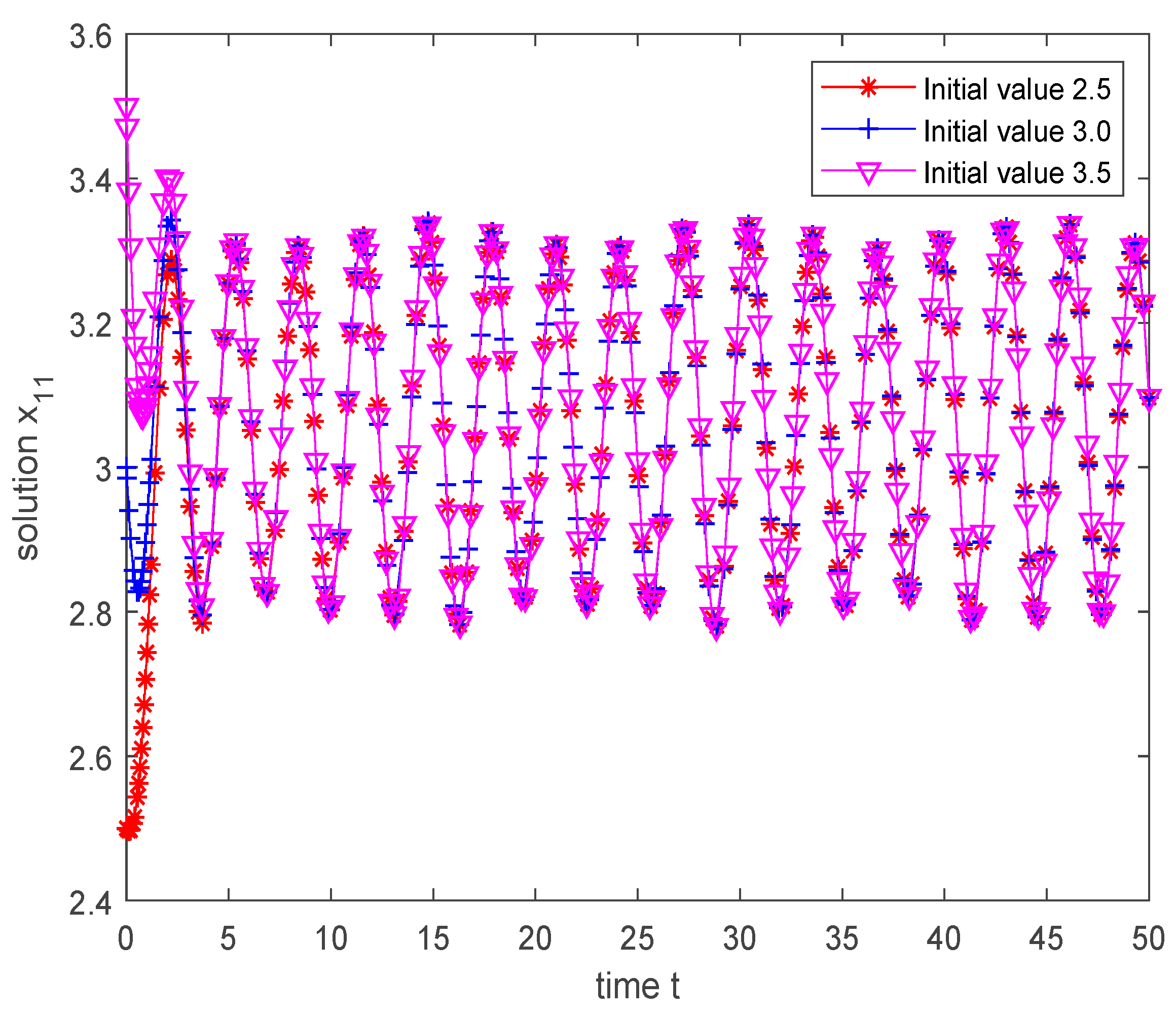
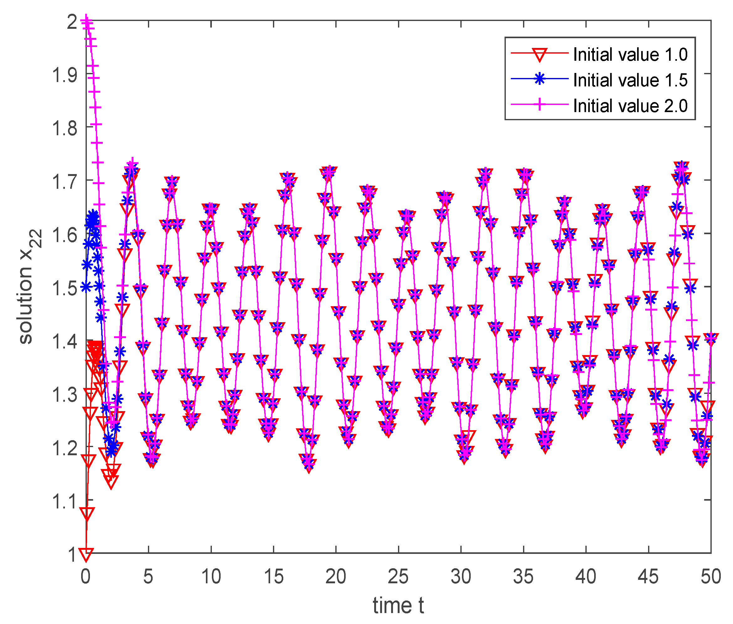
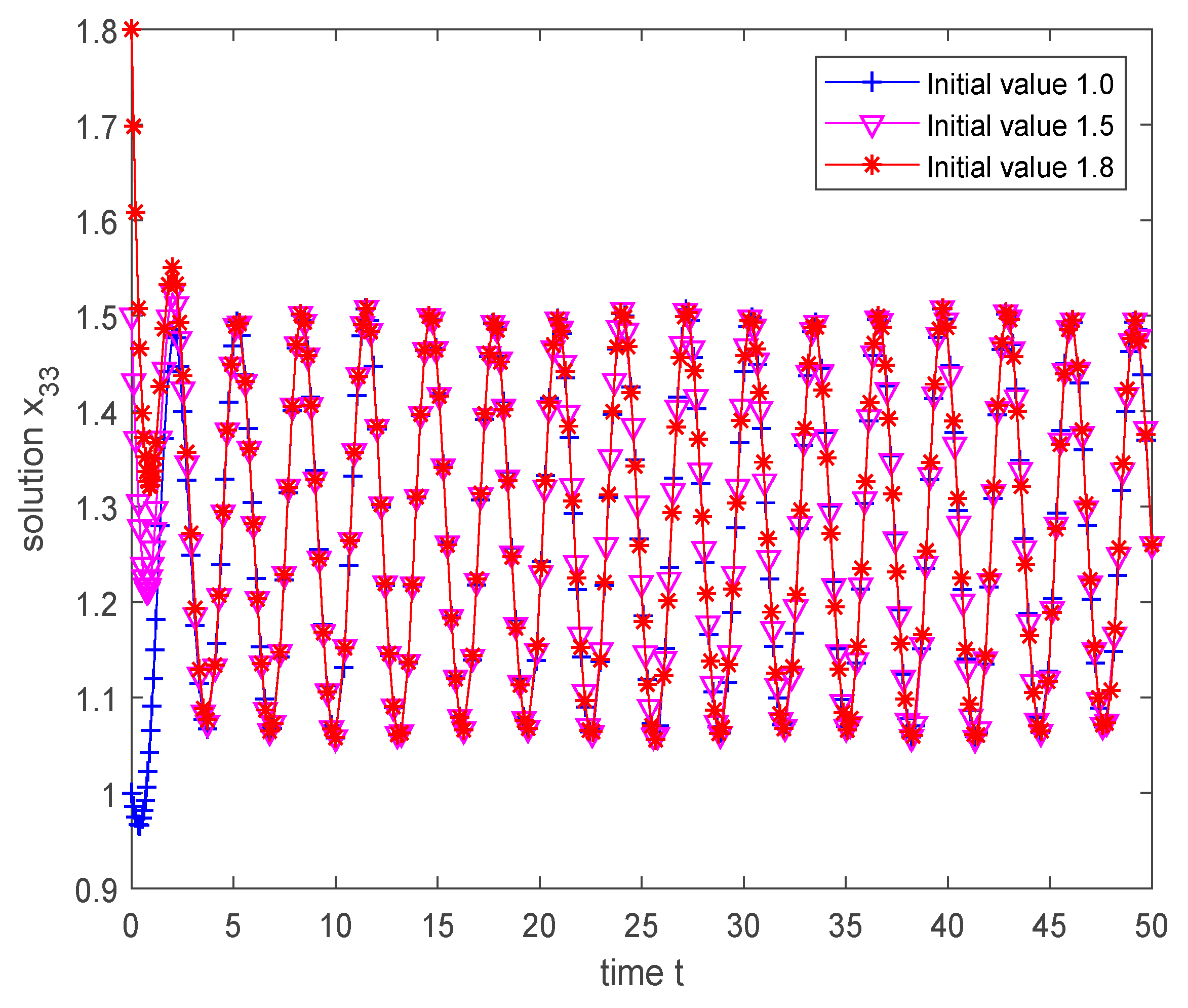
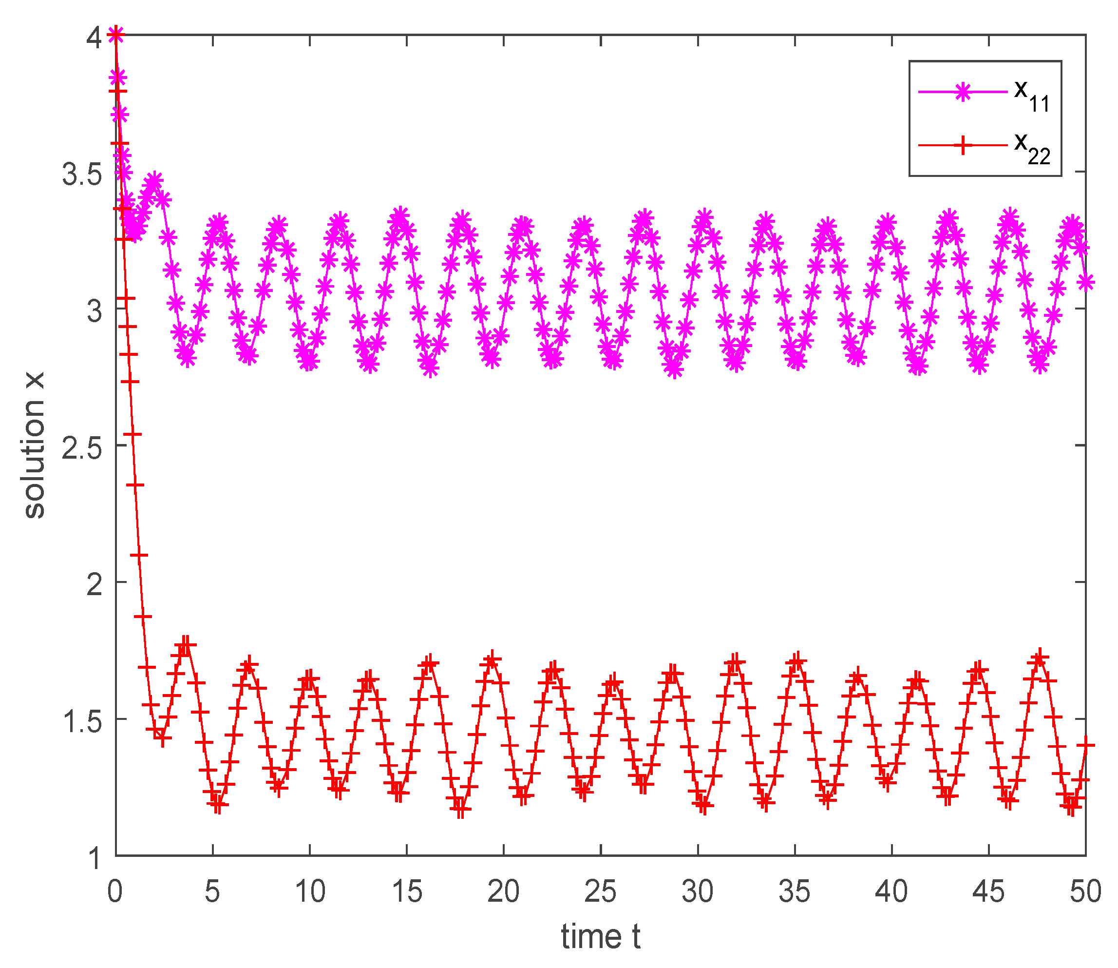
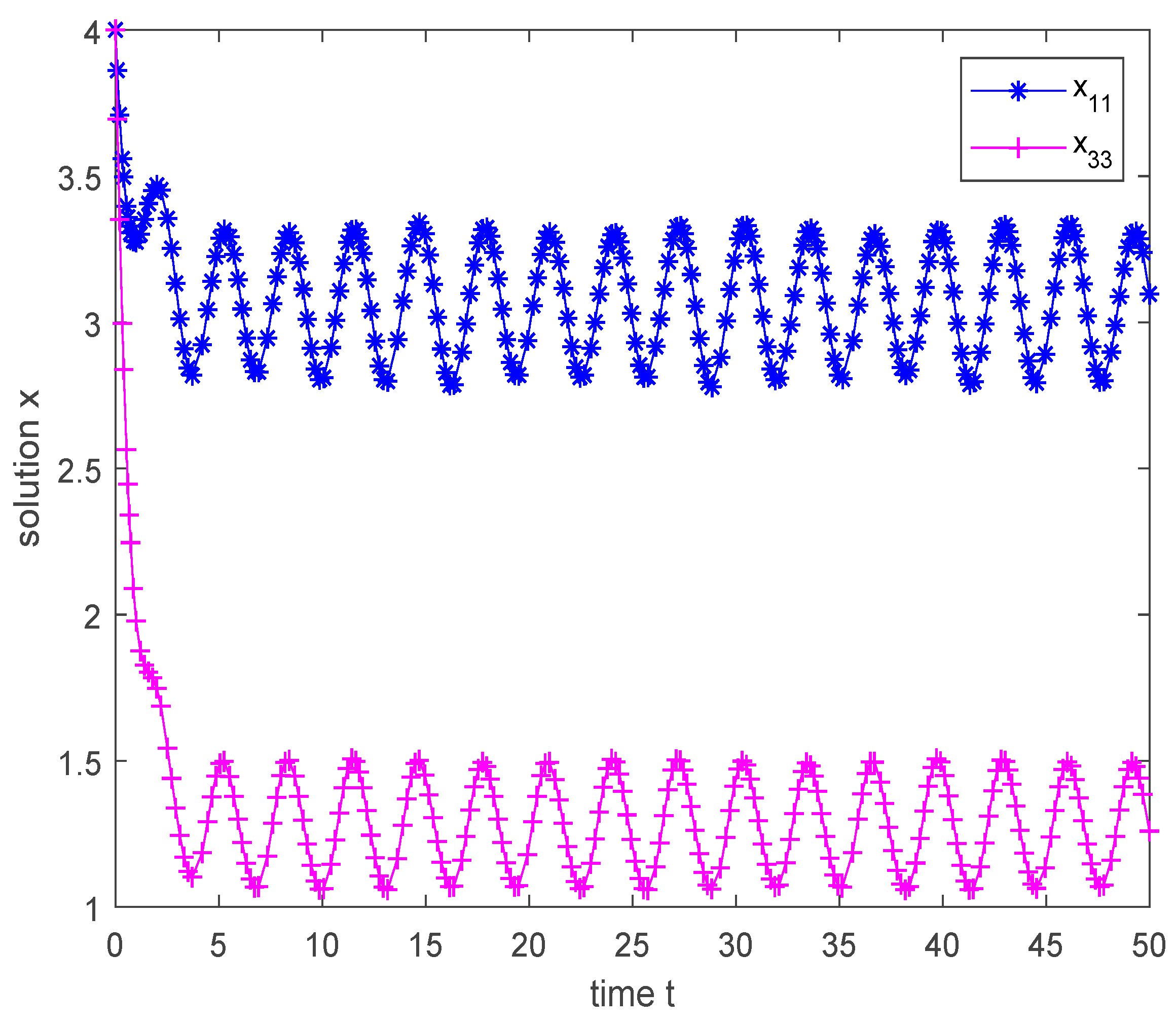
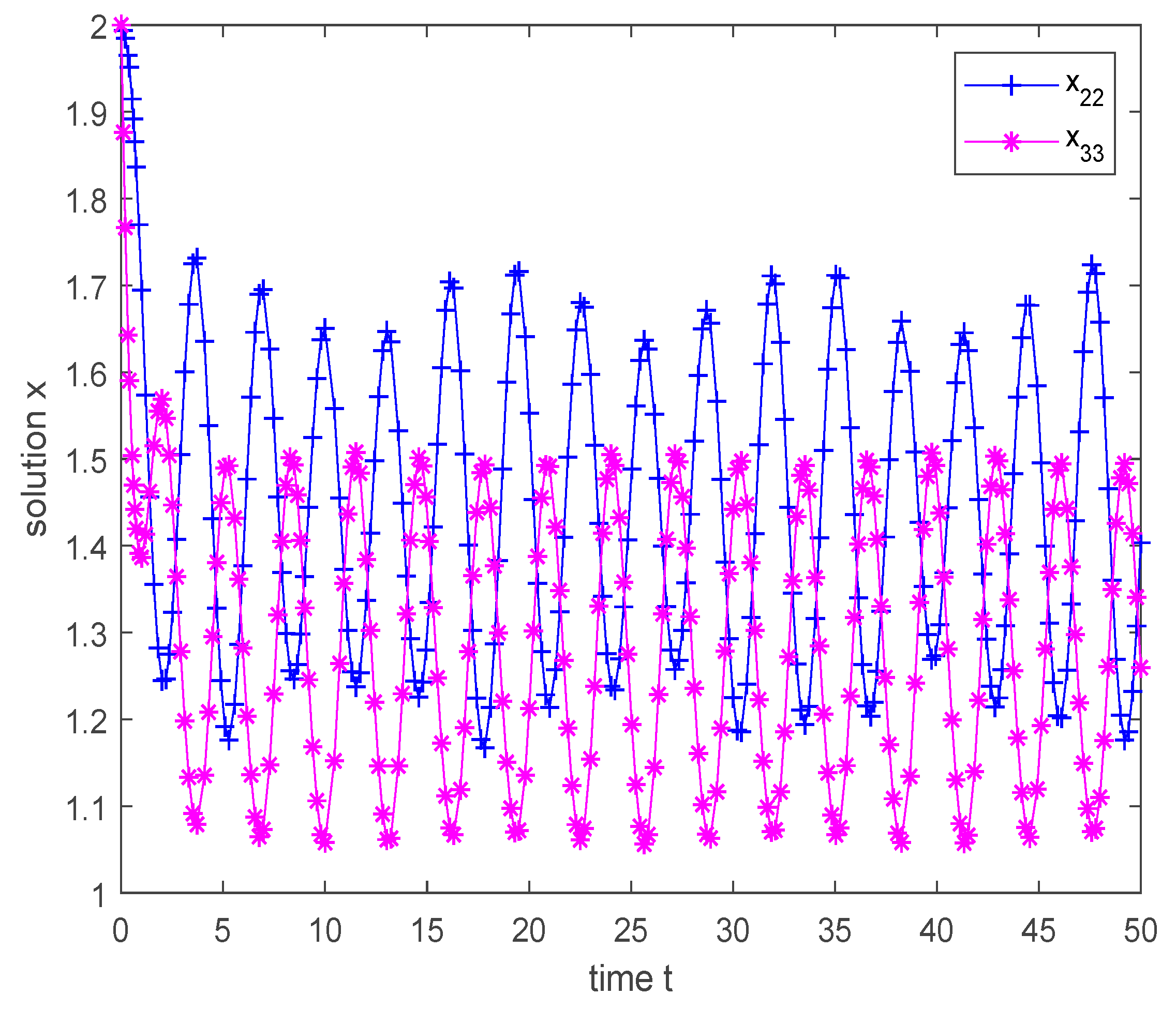
This example is simulated through MATLAB according to the given parameters. Figure 1, Figure 2, and Figure 3 display the state trajectories $x_{11}(t),x_{22}(t)$, and $x_{33}(t)$ of the pseudo-almost periodic solution for the neural network system (15) with three different initial values $(2.5,3.0,3.5),(1.0,1.5,2.0),(1.0,1.5,1.8)$, respectively. Even with the change of initial points, the shapes of the trajectories are not changed. As can be seen that simulated the solution tends to be the pseudo-almost periodic solution of the neural network system (4.1). Figure 4 shows the dynamic behavior of the pseudo-almost solution $x_{11}(t)$ and $x_{22}(t)$ of the neural network system (15) with the same initial values $x_{11}(0)=x_{22}(0)=4$. Similarly, Figure 5 exhibits the dynamic behavior of the pseudo-almost solution $x_{11}(t)$ and $x_{33}(t)$, and Figure 6 $x_{22}(t)$ and $x_{33}(t)$. The validity of the conclusions can be judged by comparing the two-state trajectories with each other.

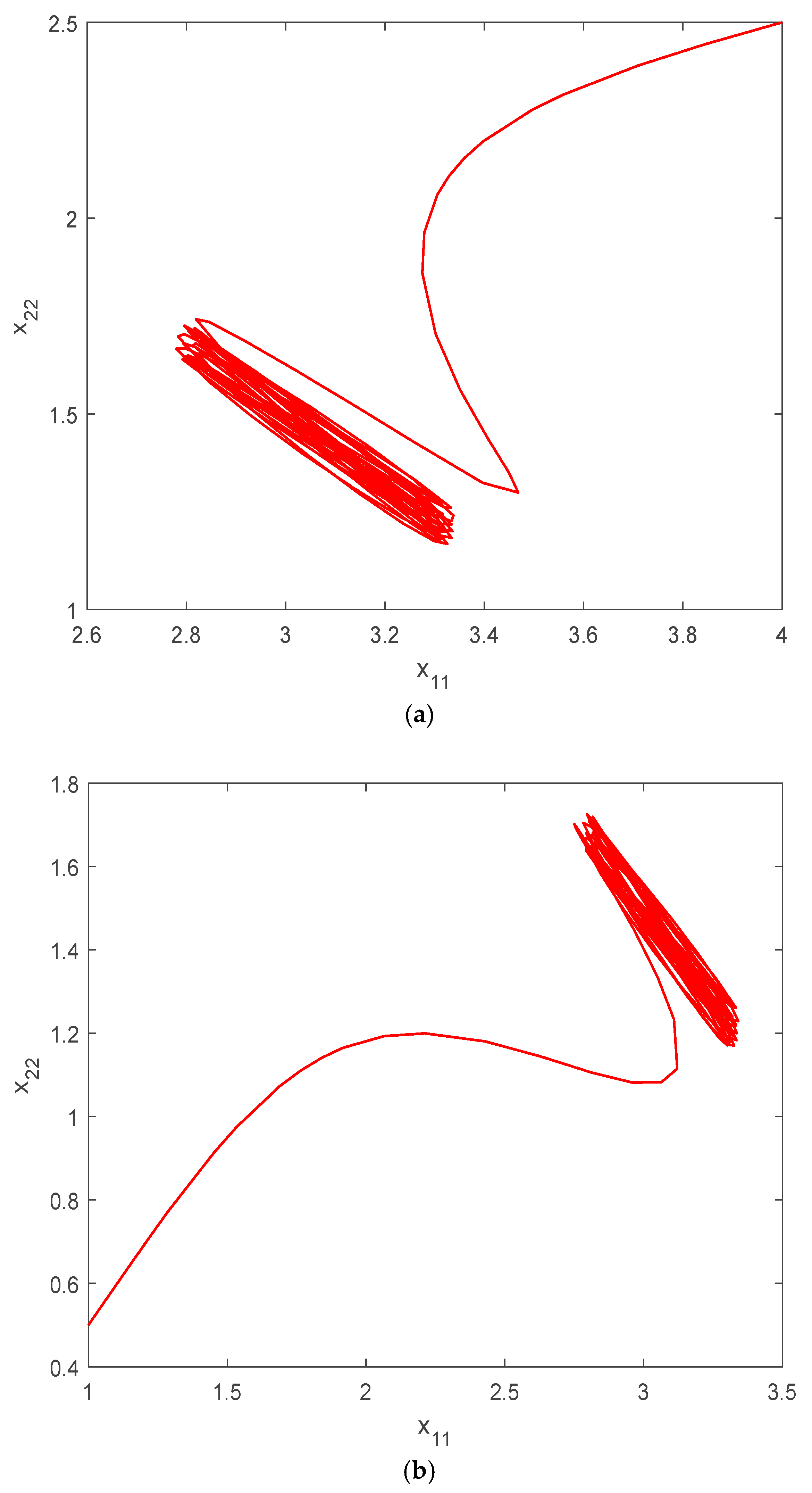
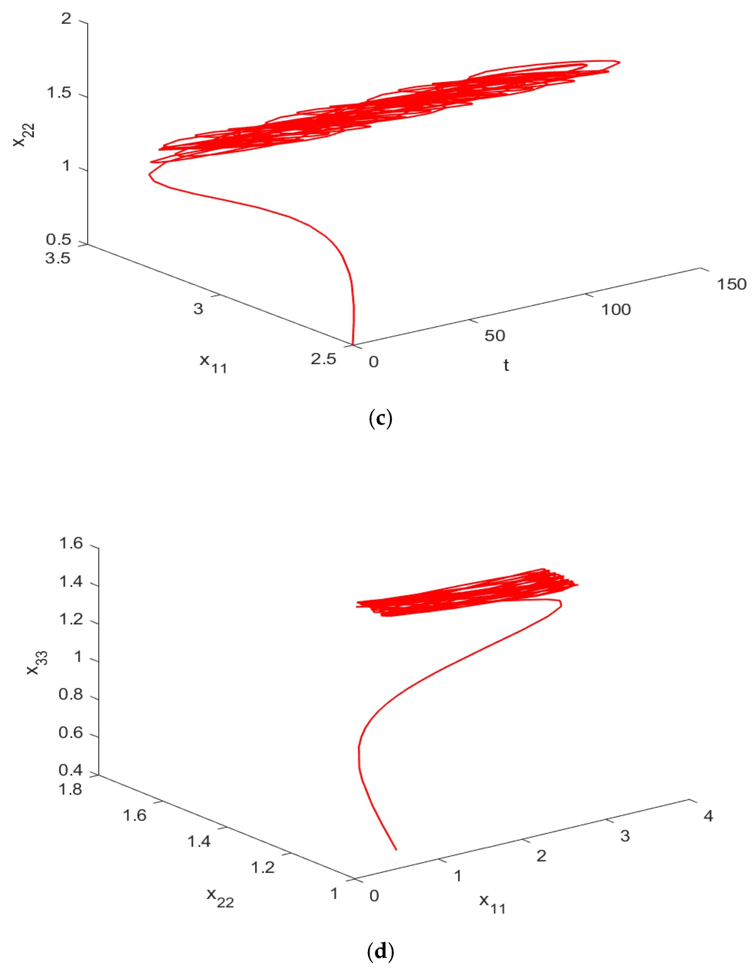
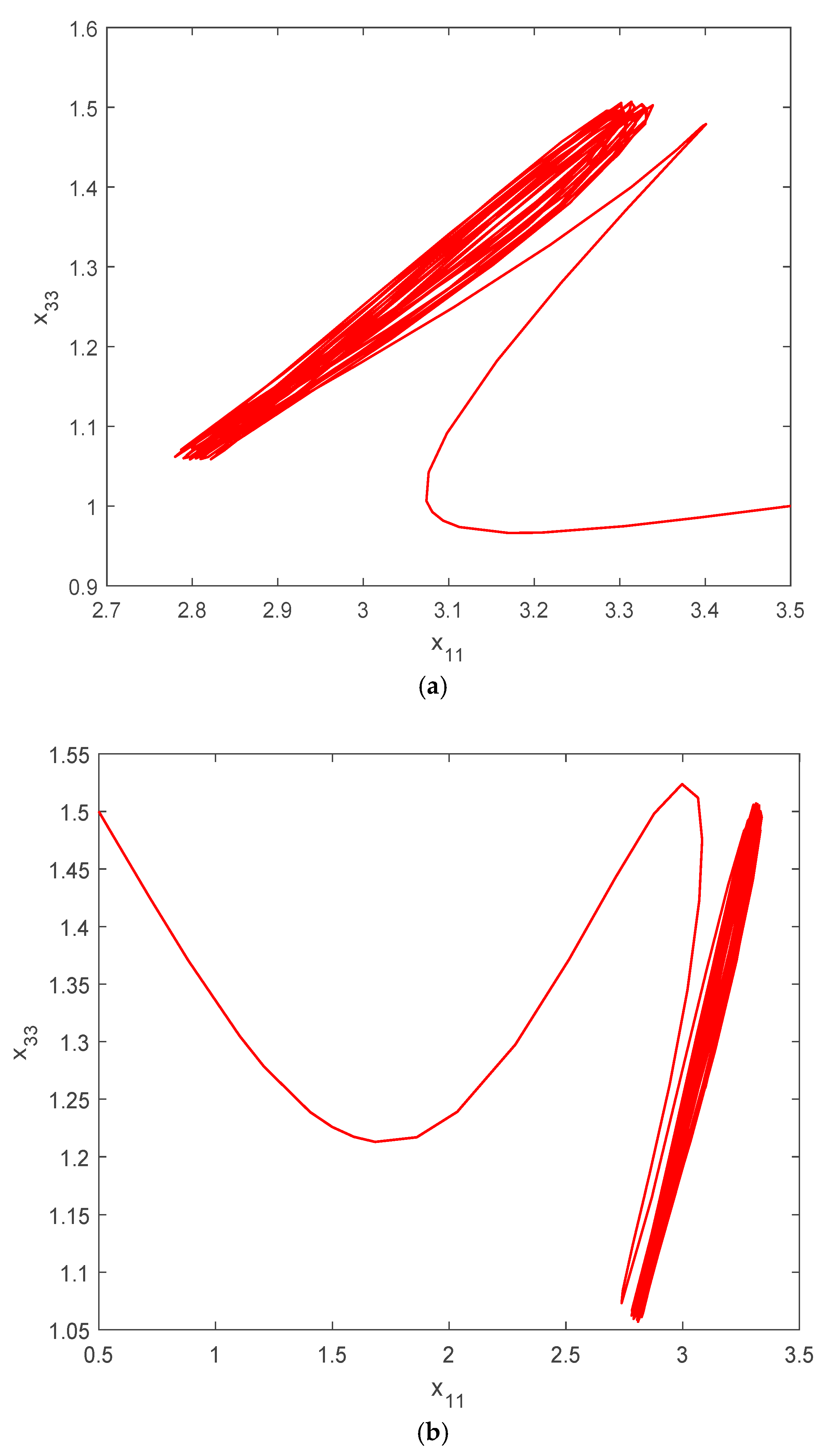
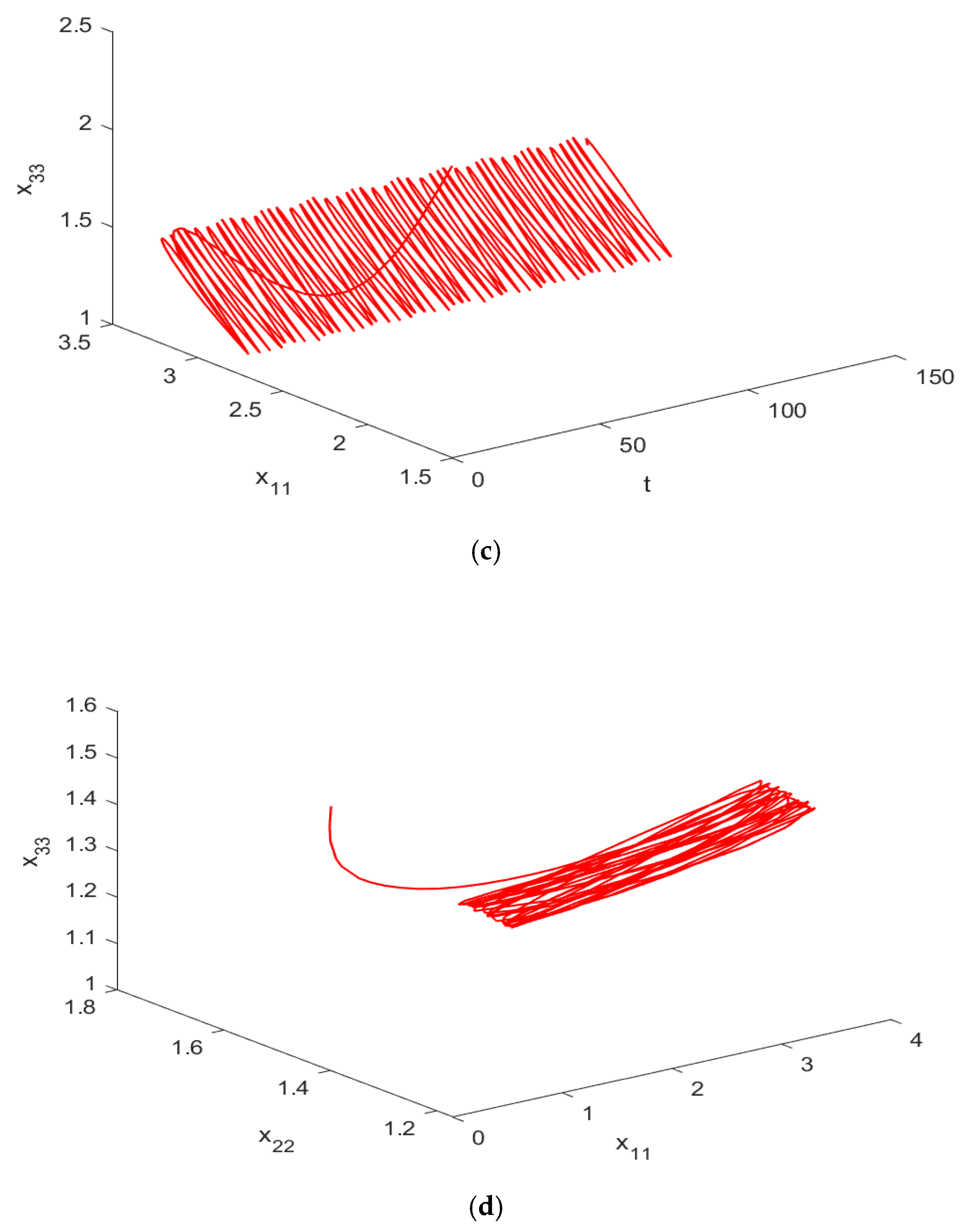
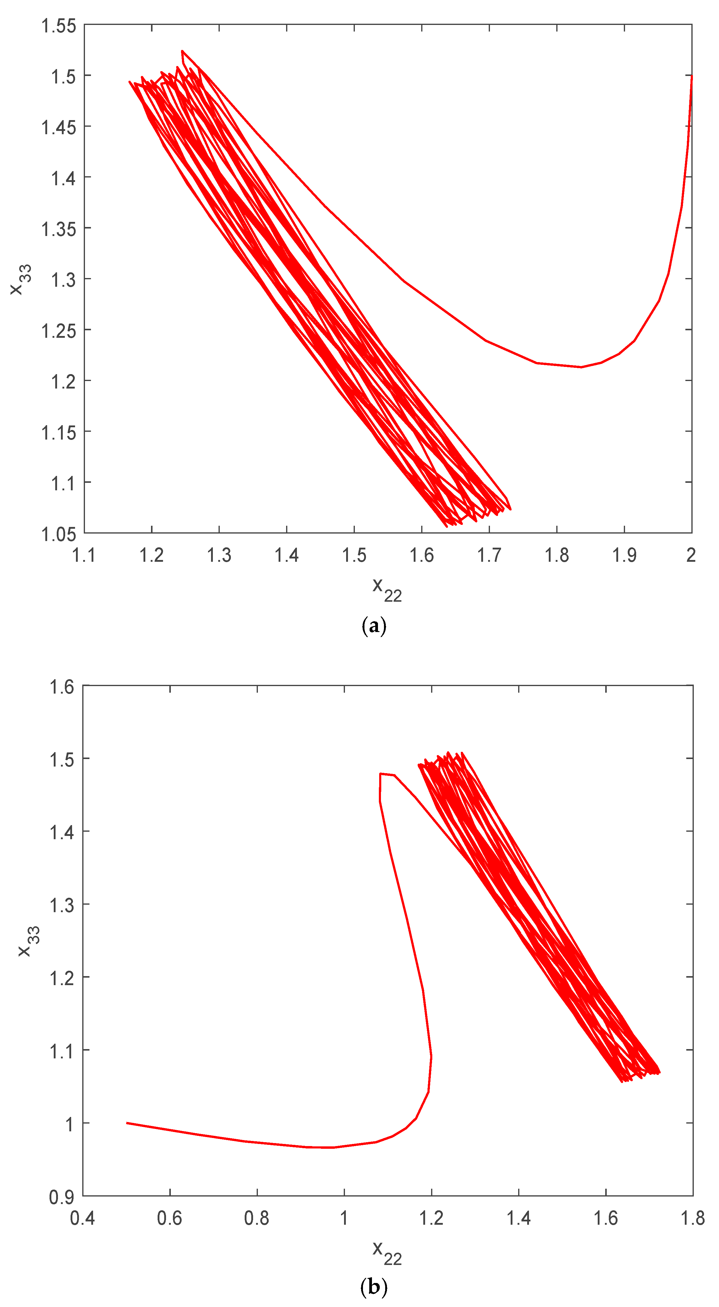
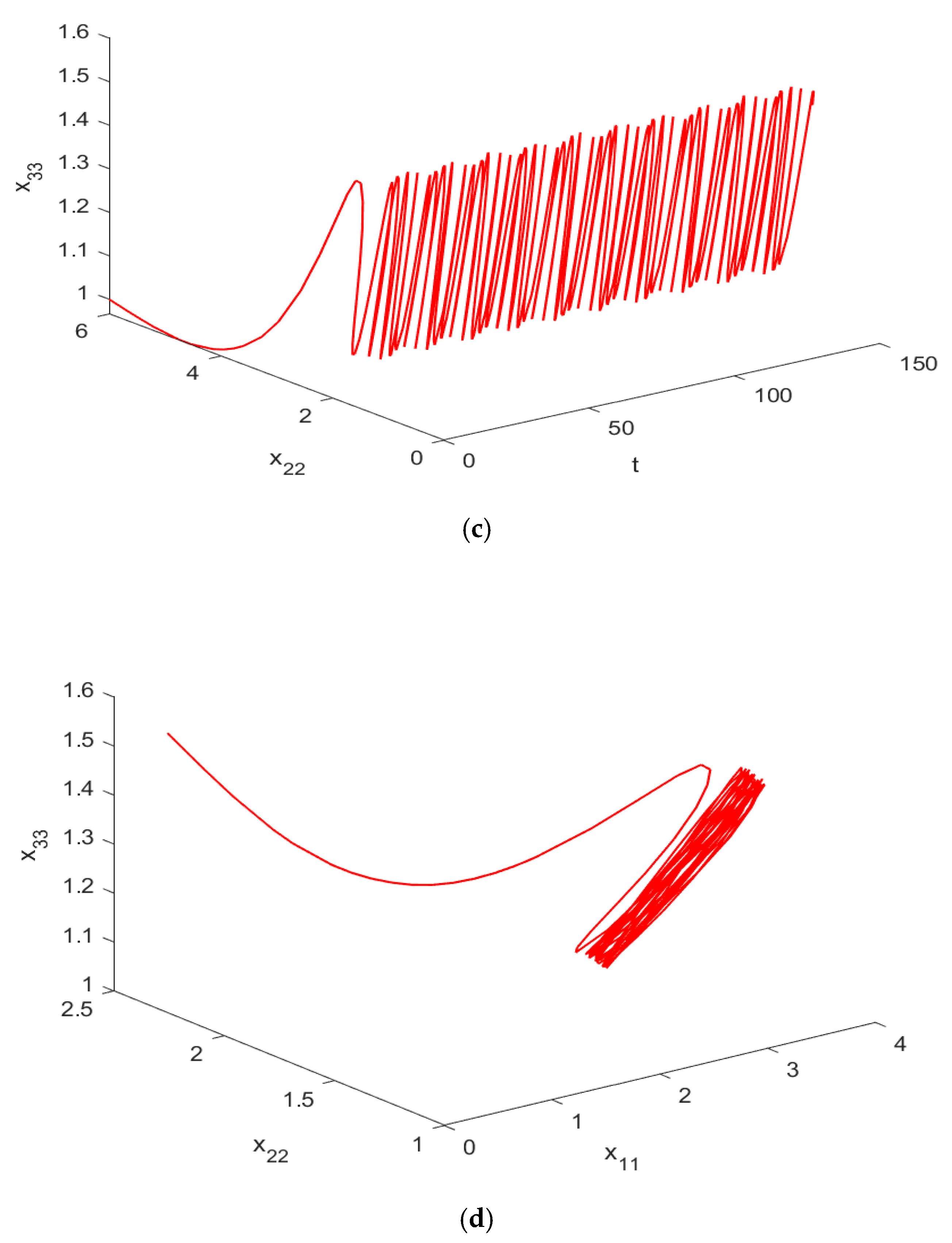
Figure 7a,b demonstrates the phase responses of state variables $x_{11}(t)$ and $x_{22}(t)$ for the neural network system (15) with different initial values $(4.0,2.5),(1.0,0.5)$. Figure 7c describes the space behavior of the state variables $x_{11}(t),x_{22}(t)$ for the neural network system (15). Similarly, Figure 8a,b shows the phase responses of state variables $x_{11}(t)$ and $x_{33}(t)$ for the neural network system (15) with different initial values $(3.5,1.0),(0.5,1.5)$. Figure 8c space behavior of the state variables $x_{11}(t)$, $x_{33}(t)$ for the neural network system (15); and Figure 9a,b depict phase diagram $x_{22}(t)$ and $x_{33}(t)$ with $(2.0,1.5),(0.5,1.0)$, Figure 9c reveals the space behavior of the state variables $x_{22}(t)$ and $x_{33}(t)$. Figure 7d, Figure 8d, and Figure 9d exhibitions the 3D space behavior of the state variables $x_{11}(t),x_{22}(t)$ and $x_{33}(t)$ for the neural network system (15) with three different initial values $(0.5,1.0,0.5),(0.5,1.5,1.5),(0.5,2.5,1.5)$. The time response confirms that our theoretical results’ sufficient conditions are effective for the neural network system (15). Moreover, the phase response represents a bunch of pseudo-almost periodic trajectories, which gives an idea of pseudo-almost periodic solutions for our described neural network system (15). Considered the above relative parameters, all the conditions of Theorems 1 and 2 are satisfied. Therefore, the neural network system (15) has precisely one continuously differential pseudo-almost periodic solution, which is also globally exponentially stable.

5. Conclusions

In this paper, the existence and stability criteria of the pseudo-almost periodic solution for the novel type complex networks are examined. Based on the Banach fixed-point theorem and the exponential dichotomy of linear equations, the existence and uniqueness of pseudo-almost periodic solutions are investigated. Through an integral variable transformation, the global exponential stability condition of the CNN is evaluated. Compared with the previous work on the stability analysis of periodic solutions, the derived pseudo-almost periodic results are more precise and less conservative. The proposed variable substitution can induce stability flexibility, overcome the bottleneck problem of constructing the complicated Lyapunov functional, and ensure the convergence results from more validity. The approach has a fast convergence speed, which is suitable for applications of complex systems. The obtained results in this work are valuable in the design of neural network systems, which are used to solve efficiency and optimal control problems arising in practical engineering applications. The existence and stability conditions are expressed in simple algebraic form, and their verification is done.

In future work, the analysis method can also be applied to more complicated neural network systems such as fuzzy systems and fractional-order neural networks that arise in the various disciplines of engineering and scientific fields. Such as, Mittag-Leffer stability of the fractional-order neural networks with discontinuous activation functions and time-varying delays will also be explored. Moreover, synchronization and state estimation of the fractional-order memristor-based neural networks and stochastic delayed systems will also be examined in the future.

References

- Chua, L.; Yang, L. Cellular neural networks: Theory. IEEE Trans. Circuits Syst. 1988, 35, 1257–1272. [Google Scholar] [CrossRef]
- Chua, L.; Yang, L. Cellular neural networks: Applications. IEEE Trans. Circuits Syst. 1988, 35, 1273–1290. [Google Scholar] [CrossRef]
- Jiang, H.; Cao, J. Global exponential stability of periodic neural networks with time-varying delays. Neurocomputing 2006, 70, 343–350. [Google Scholar] [CrossRef]
- Li, H.; Jiang, H.; Hu, C. Existence and global exponential stability of periodic solution of memristor-based BAM neural networks with time-varying delays. Neural Netw. 2016, 75, 97–109. [Google Scholar] [CrossRef]
- Yang, W.; Yu, W.; Cao, J. Global exponential stability of impulsive fuzzy high-order BAM neural networks with continuously distributed delays. IEEE Trans. Neural Netw. Learn. Syst. 2018, 29, 3682–3700. [Google Scholar] [PubMed]
- Wang, H.; Duan, S.; Huang, T.; Li, C.; Wang, L. Novel stability criteria for impulsive memristive neural networks with time-varying delays. Circuits Syst. Signal Process. 2016, 35, 3935–3956. [Google Scholar] [CrossRef]
- Wen, C.; Wang, Z.; Geng, T.; Alsaadi, F. Event-based distribute d recursive filtering for state-saturated systems with redundant channels. Inf. Fusion 2018, 39, 96–107. [Google Scholar] [CrossRef]
- Liu, Q.; Wang, Z.; He, X.; Zhou, D.H. Event-triggered resilient filtering with measurement quantization and random sensor failures: Monotonicity and convergence. Automatica 2018, 94, 458–464. [Google Scholar] [CrossRef]
- Wang, F.; Wang, Z.; Liang, J.; Yang, J. Locally minimum-variance filtering of 2-D systems over sensor networks with measurement degradations: A distributed recursive algorithm. IEEE Trans. Cybern. 2020, 99, 1–13. [Google Scholar] [CrossRef] [PubMed]
- Wang, Y.; Xia, Y.; Zhou, P.; Duan, D. A new result on H∞ state estimation of delayed static neural networks. IEEE Trans. Neural Netw. Learn. Syst. 2017, 28, 3096–3101. [Google Scholar] [CrossRef] [PubMed]
- Donkers, M.; Heemels, W.; van de Wouw, N.; Hetel, L. Stability analysis of networked control systems using a switched linear systems approach. IEEE Trans. Autom. Control 2011, 56, 2101–2115. [Google Scholar] [CrossRef] [Green Version]
- Liang, J.; Wang, Z.; Liu, X.; Louvieris, P. Robust synchronization for 2-D discrete-time coupled dynamical networks. IEEE Trans. Neural Netw. Learn. Syst. 2012, 23, 942–953. [Google Scholar] [CrossRef] [Green Version]
- Sharkovsky, A.N. Chaos from a time-delayed Chua’s circuit. IEEE Trans. Circuits Syst. I Fundam. Theory Appl. 1993, 40, 781–783. [Google Scholar] [CrossRef]
- Ge, C.; Hua, C.; Guan, X. New delay-dependent stability criteria for neural networks with time-varying delay using delay-decomposition approach. IEEE Trans. Neural Netw. Learn. Syst. 2014, 25, 1378–1383. [Google Scholar]
- Seuret, A.; Gouaisbaut, F.; Fridman, E. Stability of discrete-time systems with time-varying delays via a novel summation inequality. IEEE Trans. Autom. Control 2015, 60, 2740–2745. [Google Scholar] [CrossRef] [Green Version]
- Liang, J.; Wang, Z.; Liu, X. Exponential synchronization of stochastic delayed discrete-time complex networks. Nonlinear Dyn. 2008, 53, 153–165. [Google Scholar] [CrossRef]
- Ou, C. Almost periodic solutions for shunting inhibitory cellular neural networks. Nonlin. Anal. RWA 2009, 10, 2652–2658. [Google Scholar] [CrossRef]
- Zhang, X.; Han, Q. Global asymptotic stability for a class of generalized neural networks with interval time-varying delay. IEEE Trans. Neural Netw. 2011, 22, 1180–1192. [Google Scholar] [CrossRef]
- Gong, W.; Liang, J.; Cao, J. Matrix measure method for global exponential stability of complex-valued recurrent neural networks with time-varying delays. Neural Netw. 2015, 70, 81–89. [Google Scholar] [CrossRef]
- Miraoui, M. μ-Pseudo-Almost Automorphic Solutions for some Differential Equations with Reflection of the Argument. Numer. Funct. Anal. Optim. 2017, 38, 376–394. [Google Scholar] [CrossRef]
- Cherif, F. Sufficient Conditions for Global Stability and Existence of Almost Automorphic Solution of a Class of RNNs. Differ. Equ. Dyn. Syst. 2014, 22, 191–207. [Google Scholar] [CrossRef]
- Zhang, X.; Han, Q.; Zeng, Z. Hierarchical type stability criteria for delayed neural networks via canonical Bessel-Legendre inequalities. IEEE Trans. Cybern. 2018, 48, 1660–1671. [Google Scholar] [CrossRef]
- Saratha, S.; Sai Sundara Krishnan, G.; Bagyalakshmi, M. Analysis of a fractional epidemic model by fractional generalised homotopy analysis method using modified Riemann-Liouville derivative. Appl. Math. Model. 2021, 92, 525–545. [Google Scholar] [CrossRef]
- Liu, P.; Wang, G. Optimal periodic preventive maintenance policies for systems subject to shocks. Appl. Math. Model. 2021, 93, 101–114. [Google Scholar] [CrossRef]
- Wang, L.; Wang, Z.; Wei, G.; Alsadi, F. Finite-time state estimation for recurrent delayed neural networks with component-based event-triggering protocol. IEEE Trans. Neural Netw. Learn. Syst. 2018, 29, 1046–1057. [Google Scholar] [CrossRef] [PubMed]
- Kang, H.; Fu, X.; Sun, Z. Global exponential stability of periodic solutions for impulsive Cohen-Grossberg neural networks with delays. Appl. Math. Model. 2015, 39, 1526–1535. [Google Scholar] [CrossRef]
- Mandal, S.; Majee, N. Existence of periodic solutions for a class of Cohen-Grossberg type neural networks with neutral delays. Neurocomputing 2011, 74, 1000–1007. [Google Scholar] [CrossRef]
- Bohr, H. Zur theorie der fast periodischen funktionen: I. eine verallgemeinerung der theorie der fourierreihen. Acta Math. 1925, 45, 29–127. [Google Scholar] [CrossRef]
- Shao, J.; Wang, L.; Ou, C. Almost periodic solutions for shunting inhibitory cellular neural networks without global Lipschitz activaty functions. Appl. Math. Model. 2009, 33, 2575–2581. [Google Scholar] [CrossRef]
- Wang, K.; Zhu, Y. Stability of almost periodic solution for a generalized neutral-type neural networks with delays. Neurocomputing 2010, 73, 3300–3307. [Google Scholar] [CrossRef]
- Zhang, C. Pseudo Almost Periodic Functions and Their Applications. Ph.D. Thesis, University of Western Ontario, London, ON, Canada, 1992. [Google Scholar]
- Ding, H.; Liang, J.M.; N’Guérékat, G.; Xiao, T. Pseudo-almost periodicity of some nonautonomous evolution equations with delay. Nonlinear Anal. Theory Methods Appl. 2007, 67, 1412–1418. [Google Scholar] [CrossRef]
- Mhamdi, M.; Aouiti, C.; Touati, A. Weighted pseudo almost-periodic solutions of shunting inhibitory cellular neural networks with mixed delays. Acta. Math. Sci. 2016, 36, 1662–1682. [Google Scholar] [CrossRef]
- Amdouni, M.; Cherif, F. The pseudo almost periodic solutions of the new class of Lotka-Volterra recurrent neural networks with mixed delays. Chaos Solut. Fractals 2018, 113, 79–88. [Google Scholar] [CrossRef]
- Liu, B. Pseudo almost periodic solutions for neutral type CNNs with continuously distributed leakage delays. Neurocomputing 2015, 148, 445–454. [Google Scholar] [CrossRef]
- Shao, J. Pseudo almost periodic solutions for a Lasota-Wazewska model with an oscillating death rate. Appl. Math Lett. 2015, 43, 90–95. [Google Scholar] [CrossRef]
- Zhang, A. Almost Periodic Solutions for SICNNs with Neutral Type Proportional Delays and D Operator. Neural Process Lett. 2018, 47, 57–70. [Google Scholar] [CrossRef]
Figure 1.
The state trajectory of , and initial values are respectively.
Figure 2.
Figure 3.
Figure 4.
The state trajectory of and , and initial values are .
Figure 5.
Figure 6.
Figure 7.
The state trajectory of , 3D graphs and initial values are (a) (b) (c) and (d) respectively.
Figure 8.
Figure 9.
Publisher’s Note: MDPI stays neutral with regard to jurisdictional claims in published maps and institutional affiliations. |
© 2021 by the authors. Licensee MDPI, Basel, Switzerland. This article is an open access article distributed under the terms and conditions of the Creative Commons Attribution (CC BY) license (https://creativecommons.org/licenses/by/4.0/).
Share and Cite
MDPI and ACS Style
Liu, W.; Huang, J.; Yao, Q. Stability Analysis of Pseudo-Almost Periodic Solution for a Class of Cellular Neural Network with D Operator and Time-Varying Delays. Mathematics 2021, 9, 1951. https://doi.org/10.3390/math9161951
AMA Style
Liu W, Huang J, Yao Q. Stability Analysis of Pseudo-Almost Periodic Solution for a Class of Cellular Neural Network with D Operator and Time-Varying Delays. Mathematics. 2021; 9(16):1951. https://doi.org/10.3390/math9161951
Chicago/Turabian StyleLiu, Weide, Jianliang Huang, and Qinghe Yao. 2021. "Stability Analysis of Pseudo-Almost Periodic Solution for a Class of Cellular Neural Network with D Operator and Time-Varying Delays" Mathematics 9, no. 16: 1951. https://doi.org/10.3390/math9161951
Note that from the first issue of 2016, this journal uses article numbers instead of page numbers. See further details here.