Classification of Diseases Using Machine Learning Algorithms: A Comparative Study

Abstract

Machine learning in the medical area has become a very important requirement. The healthcare professional needs useful tools to diagnose medical illnesses. Classifiers are important to provide tools that can be useful to the health professional for this purpose. However, questions arise: which classifier to use? What metrics are appropriate to measure the performance of the classifier? How to determine a good distribution of the data so that the classifier does not bias the medical patterns to be classified in a particular class? Then most important question: does a classifier perform well for a particular disease? This paper will present some answers to the questions mentioned above, making use of classification algorithms widely used in machine learning research with datasets relating to medical illnesses under the supervised learning scheme. In addition to state-of-the-art algorithms in pattern classification, we introduce a novelty: the use of meta-learning to determine, a priori, which classifier would be the ideal for a specific dataset. The results obtained show numerically and statistically that there are reliable classifiers to suggest medical diagnoses. In addition, we provide some insights about the expected performance of classifiers for such a task.

1. Introduction

Supervised learning is one of the most common and important paradigms in pattern recognition, with pattern classification being one of the most important tasks [1]. In this context, in the state of the art situation, there are methods of pattern classification which are useful for classifying patterns in different application areas [2].

Pattern classification has become very important for decision making in many areas of human activity and the medical area is no exception. Researchers in machine learning have been designing new classification algorithms for this purpose, seeking a classification efficiency close to 100%. It is important to emphasize that there is no perfect classifier. This fact is guaranteed by the No-Free-Lunch theorem, which governs the effectiveness of classifiers [3,4]. This theorem has motivated machine learning researchers to design novel classification algorithms, with the property that of exhibiting the fewest possible errors [5,6].

This work aims to focus on classification algorithms that are useful for effective diagnosis of medical diseases. This area is of utmost importance because a good diagnosis will significantly improve the life of the patient. An example: based on a chest radiograph, a classifier can correctly decide whether a patient corresponds to a patient suffering from pneumonia or corresponds to a healthy person [7], assuming that only these two classes exist. Obviously, the correct classification depends on the algorithm classifier, that is, how good it is, and the complexity of the database. In the medical area, it is very important to have computer tools that help the health professional to diagnose diseases in a timely manner. In addition, it is very important to have data whose quality is guaranteed. In this regard, over time various international dataset repositories have been formed, which are very useful to the scientific community in machine learning and related areas. Fortunately for our work, in these repositories there is a number of medical datasets, which are the raw material for studies such as the one reported in this article.

In this research work, three widely used repositories have been chosen: Kaggle (https://www.kaggle.com/, accessed on 30 May 2021), the University of California Machine Learning Repository [8], and the KEEL repository [9]. In these repositories there are datasets of patterns of medical diseases, and they offer balanced and unbalanced data, a very important fact, because the classification algorithms, in this situation, have a marked bias towards the majority class and practically ignore the minority class [10,11]. In this article we will use 23 datasets that are classified into five categories of medical diseases: heart disease conformed for six datasets, cancer related diseases with seven datasets, diabetes related diseases with two datasets, thyroid diseases with two datasets, and finally several diseases with six datasets.

The classification algorithms used in the present work are: Multilayer Perceptron (MLP), Naïve Bayes (NB), K Nearest Neighbors (KNN), decision trees (C4.5), logistic regression (Logistic), Support Vector Machines (SVM) and Deep Learning (DL). In addition, we tested several measures of data complexity, in order to a priori determine the expected performance of the compared classifiers for medical datasets [2,11].

In machine learning, researchers in this area have platforms on which they can test classification algorithms or develop their pattern classification algorithms. One of these platforms is WEKA [12], which due to its usefulness and easy handling is a well-known machine learning platform. WEKA was developed in New Zealand at the University of Waikato and can be downloaded at www.cs.waikato.ac.nz/ml/weka/, accessed on 30 May 2021. It contains a comprehensive collection of predictive models and data analysis algorithms that include methods that address regression problems, feature selection, clustering, and classification. WEKA’s flexibility allows the preprocessing and management of a data set in a learning schema and then analysis of the performance of the classifier in use. WEKA was programmed in Java. The classification algorithms used in this paper are part of the vast set of algorithms that WEKA includes. Another platform for experimentation is KEEL [9,13], developed by the University of Granada in Spain, which also includes data complexity measures.

The paper is structured as follows: Section 2 includes important state-of-the-art works dealing with the classification of medical patterns. In Section 3 the experimental setup is explained, including the selected datasets and classifiers, as well as the data complexity and performance measures. Section 4 is very important because it describes and discusses several highly relevant aspects: first, the numerical and statistical behavior of the classifiers is widely described and discussed, and then meta-learning techniques are applied. The results obtained allow us to crystallize the purpose of this article: with the results obtained from the meta-learning techniques, we will be able to propose the best classifiers for the diagnosis of specific diseases. Finally, Section 5 presents the conclusions derived from the present research.

2. Previous Works

The Free Lunch Theorem guarantees that there is no perfect classifier. Therefore, machine learning researchers are now looking for the fewest errors in their algorithms. For example, in [14], the authors added the K-NN algorithm to a distance function that is sensitive to cost, through a careful selection of the K parameter. Another example of performance improvement in classifiers is the case of the multilayer perceptron to find the appropriate number of hidden units [15].

A framework for classifying lung problems is described in [16]. In this work, a tuberculosis dataset and different configurations were used for the semi-supervised learning algorithms, such as co-training, tri-training and self-taught. Another example of the use of classifiers in the medical area is found in [17]. Here, the authors manually obtained the characteristics of Magnetic Resonance Imaging (MRI) and used them in a linear regression algorithm for classification in brain damage in patients.

Deep Learning methods, with special emphasis on Convolutional Neural Networks (CNN), are widely used for the classification and segmentation of medicinal images. Here are some notable recent examples. A detailed description of how computer-aided diagnosis is helpful in improving clinical care, is included in [18]. The detection of glaucoma through the classification of processed images is shown in [19]. A method of classification of lesions in a hemorrhagic stroke using a CNN is shown in [20]. An automatic system based on a CNN to detect discs of the lumbar spine is proposed in [21]. A model based on a CNN to improve the classification of Papanicolaou smears is proposed in [22]. An automatic model called online transfer learning is proposed in [23] for the differential diagnosis of benign and malignant thyroid nodules from ultrasound images. The content of reference [24] does not include the use of CNN. In this research work, a new associative pattern classification algorithm called Lernmatrix tau 9 is introduced, which is applied to medical datasets.

COVID-19 has been one of the strongest health problems in the last two years and is an area of interest not only in the medical area but also in machine learning. Classification algorithms, such as convolutional neural networks, have been widely used to provide a useful diagnosis to healthcare professionals [25,26,27,28,29,30,31,32,33,34,35,36,37,38,39].

As can be seen, the classification of patterns of medical diseases is of great interest to the scientific community in machine learning and to health professionals. Interest is great in the classification of algorithms, not only for the creation of new algorithms that reduce the error in classification, but also for existing classification algorithms. It is important to know the behavior of pattern classifiers in the state of the art examples, because knowing the performance of the classification algorithms can be very helpful in diagnosing clinical diseases. It is evident and undeniable how valuable it can be for a medical team to know in advance (with scientifically substantiated reasons) which classifier or group of classifiers is the most appropriate for the diagnosis of a specific disease. Hence the relevance of this work, from which the results obtained can have benefits on the quality of peoples’ lives.

3. Experimental Setup

We wanted to determine a priori if some of the well-established state of the art classifiers will perform good or poorly for specific diseases. To do so, we have tested the classifiers over 23 medical datasets, and we have computed 12 data complexity measures for such datasets. Then, for each classifier, what proceeds is the calculation of three performance measures (Balanced Accuracy, Sensitivity and Specificity), and the conversion of these results (by discretization) into three categorical values: Good, Regular, and Poor.

At this point, we were able to create a new dataset for each classifier, whose nature is totally different from the initial datasets. The patterns of this new dataset for each classifier are made up of the 12 complexity measures already calculated as input, and the discretized performance as output.

Finally, the meta-learning process comes into action, which will allow medical teams to obtain the greatest social benefit and impact from this research work on machine learning. To perform this meta-learning process, we train a decision tree.

The experimental setup is shown in Figure 1.

The first three stages of the experimental setup are shown in the following Sections, while the remaining five stages are explained in the Results section.

3.1. Datasets

We selected 23 datasets from three international repositories:

• University of California Machine Learning Repository (UCI) [8],
• Kaggle repository (https://www.kaggle.com/, accessed on 30 May 2021)
• KEEL repository [9].

These 23 datasets belong to five of the most important different subgroups of human diseases: heart diseases, cancer related diseases, diabetes, thyroid diseases and, finally, other diseases. In the following, we provide a brief description of the selected datasets.

3.1.1. Datasets for Heart Diseases

Cleveland dataset: this is heart disease dataset provided by the Medical Center, Long Beach, and the Cleveland Clinic Foundation, located in the Keel repository. It has 13 attributes, five classes, and 303 instances.

Heart Statlog dataset: this dataset that was taken from the Keel repository is intended to detect the absence (class 1) or the presence (class 2) of heart diseases in patients. It is made up of 13 attributes, 270 instances and two classes.

Heart 2 dataset: this dataset has 14 attributes, 303 instances, and two classes. Classes refer to the presence of heart disease in the patient. They have integer values from 0 to 4, where 0 means no heart problems. This dataset was taken from the Kaggle repository.

Heart failure dataset: this dataset is designed for machine learning, and contains information that allows the prediction of survival of patients with heart failure only from serum creatinine and ejection fraction. This dataset was taken from the Kaggle repository and is conformed of 13 attributes, 299 instances and two classes.

Saheart dataset: this is a South African Hearth dataset. Taken from the Keel repository, it contains information on men at high risk for coronary heart disease from a region of the Western Cape, South Africa. The result of the classification should indicate whether the patient has coronary disease. The class values are negative (0) or positive (1). It is made up of nine attributes, 462 instances and two classes.

SPECT cardiac dataset: this dataset describes cardiac imaging based on single proton emission computed tomography (SPECT). To use this dataset in atomic learning, the original SPECT images were processed to extract the characteristics that define cardiac problems in patients. The dataset was taken from the UCI repository and is made up of 22 attributes, 267 instances and two classes. The classes indicate whether the patient has (1) or does not have (0) heart problems.

3.1.2. Datasets for Cancer

Breast dataset: this dataset consists of nine attributes, two classes, and 286 instances. The attributes are age, menopause, tumor-size, inv-nodes, node -caps, deg-malig, breast, breast-quad, and irradiated. This dataset is in the Keel repository.

Haberman’s Survival dataset. The information in this dataset is used to determine if the patient survived breast cancer for periods greater than 5 years (positive) or if the patient died within 5 years (negative). The information comes from a study that was conducted at the University of Chicago Billings Hospital between 1958 and 1970. It consists of three attributes, 306 instances, and two classes. Haberman’s dataset was taken from the Keel repository.

Lymphography dataset: this dataset is widely used in machine learning. The information in the dataset is intended to detect a lymphoma and its current state. This dataset was taken from the Keel repository. It is made up of 18 attributes, 148 instances, and four classes.

Mammographic dataset. Data were obtained between 2003 and 2006 at the Institute of Radiology of the University of Erlangen-Nuremberg. The information is often used to predict the severity of a massive mammographic injury from BI-RADS attributes and the age of the patient. The classification will be benign or malignant. This dataset was taken from the Keel repository and is made up of five attributes, 961 instances, and two classes.

Primary tumor dataset: this dataset contains information on primary tumors in people. The intent is to classify the patterns or records into the class of “metastasized” or “not metastasized” to a part of the body other than where the tumor first appeared. The dataset was taken from the UCI repository and contains 339 instances, 17 attributes, and 21 classes.

Wisconsin dataset: this is an original breast cancer data set, study conducted by University of Wisconsin Hospitals. The information contained in this dataset makes it possible to classify whether the tumor detected is benign (2) or malignant (4) for patients who underwent surgery for breast cancer. The dataset was taken from the Keel repository and contains nine attributes, 699 instances, and two classes.

Wisconsin diagnosis for breast cancer 2 dataset (BCWD2). The attributes of this dataset are obtained from digitized images of breast masses generated by a fine needle aspiration (FNA) process. The extracted characteristics define the cell nuclei present in the image. The dataset was taken from the Kaggle repository. It is made up of 32 attributes, 569 instances and two classes. The distribution of the classes in the dataset are 357 benign and 212 malignant.

3.1.3. Datasets for Diabetes

Diabetes dataset: this dataset has the purpose of classifying information into two possible classes: negative test and positive test, i.e., a patient has or does not have diabetes. The dataset has 578 instances, 20 attributes, and two classes. This dataset was taken from the UCI repository and it was adapted in: https://github.com/renatopp/arff-datasets/blob/master/classification/diabetes.arff, accessed on 30 May 2021.

Pima Indians Diabetes dataset: this dataset contains information to classify or predict whether women of Pima Indian descent under the age of 21 have diabetes or not, i.e., tested negative or tested positive. This data set was taken from the Keel repository and is made up of eight attributes, 768 instances and two classes.

3.1.4. Datasets for Thyroid Diseases

Newthyroid dataset: this is a new dataset on thyroid disease. It is taken from the Keel repository and is also available from the UCI repository. The information contained in this dataset is used to predict or classify whether a patient is normal (1) or suffers from hyperthyroidism (2) or hypothyroidism (3). It is formed from five attributes, 215 instances, and three classes.

Thyroid diseases dataset: this dataset is taken from the Keel repository and is also available from the UCI repository. The information contained is used to predict or classify whether a patient is normal (1) or suffers from hyperthyroidism (2) or hypothyroidism (3). It is formed from 21 attributes, 7200 instances, and three classes.

3.1.5. Datasets for Other Diseases

Appendicitis dataset: this is a dataset taken from the Keel repository that consists of seven attributes, 106 patient instances or patterns and two classes (0,1), which represent whether the patient has appendicitis or not.

Audiology dataset (standardized)@ this dataset, extracted from the UCI repository, contains information on hearing problems in patients. The dataset is made up of 226 instances, 69 attributes, and 22 classes.

Contraceptive method choice dataset: this dataset is based on the 1987 Indonesian national survey. The samples are from single or married women who do not know if they are pregnant when interviewed. With this dataset, an attempt is made to predict which contraceptive method a woman would use according to her demographic and socioeconomic characteristics. The categories for prediction are no use, long-term methods or short-term methods. It is made up of nine attributes, 1473 instances, and three classes. This dataset was taken from the Keel repository.

Dermatology dataset: this was taken from the Keel repository. The information contained in this dataset is derived from the differential diagnosis of erythemato-squamous diseases. It is formed of 34 attributes, 366 instances, and six classes.

Ecoli dataset. The goal of this dataset is to predict the place where proteins are located using metrics about the cell, for example, cytoplasm, inner membrane, peris-plasm, outer membrane, outer membrane lipoprotein, inner membrane of inner membrane lipoprotein, cleavable signal sequence. Dataset is formed of seven attributes, 336 instances, and eight classes. The dataset was taken from the Keel repository.

Hepatitis dataset. This was taken from the Keel repository and is intended to predict whether patients affected by hepatitis will die (class 1) or survive (class 2). The dataset is made up of 19 attributes, 155 instances, and two classes.

In classification problems, a very important aspect concerning classes is knowing whether they are balanced or unbalanced. Ideally, classes should have the same instances number. Nevertheless, the most interesting data sets are unbalanced.

To exemplify, in the classification of diseases, the sick class is the minority class, and the healthy class is the majority, but the point of view of the unbalanced in the classes will affect the way of measuring the performance of the classifiers [40].

Given that most medical datasets exhibit a certain degree of imbalance in their classes, it is necessary to choose appropriate performance measures for this type of dataset, such as Balanced Accuracy, Sensitivity and Specificity. It is necessary to clarify that, in these cases, one of the most popular performance measures is not useful: accuracy [11].

Table 1. Description of the datasets.

Dataset	Classes	Attributes	Instances
appendicitis	2	7	106
audiology	22	69	226
breast	2	9	286
BCWD2	2	32	569
Cleveland	5	13	303
contraceptive	3	9	1473
dermatology	6	34	366
diabetes	2	20	578
E coli	8	7	336
Haberman	2	3	306
heart Statlog	2	13	270
heart	2	14	303
heart failure	2	13	299
hepatitis	2	19	155
lymphography	4	18	148
mammographic	2	5	961
New thyroid	3	5	215
Pima	2	8	768
primary tumor	21	17	339
saheart	2	9	462
spect train	2	22	267
thyroid	3	21	7200
Wisconsin	2	9	699

summarizes the characteristics of the 23 medical disease datasets described above.

3.2. Classifiers under Study

3.2.1. Multilayer Perceptron (MLP)

This neural network attempts to solve classification problems when classes are not linearly separable. MLP typically consists of three types of layer, the input layer, the hidden layers, and the output layer [41]. In the output layer are the neurons whose output values belong to the corresponding class. As a propagation rule, the neurons of the hidden layer occupy the weighted sum of the inputs with the synaptic weights, and a sigmoid-type transfer function is applied to this sum. The backpropagation error as a cost function uses the mean square error. Researchers in machine learning consider ML to be a very good pattern classifier.

3.2.2. C4.5 Classifier

This is a decision tree type classification algorithm. This type of classifier is among the most commonly used in classifying patterns. The C4.5 [42] is derived from an old type of decision tree called ID3 [43]. Among the parameters of the C4.5 classifier, the level of confidence for the pruning of the generated tree stands out, because it significantly influences the size and predictability of the created tree. The algorithm could be explained as follows: the predictor variable is sought to make the decision about the cut made in iteration n, in addition to the exact cut-off point where the error made is lowest, taking a pre-established variable as a criterion. This would be done as long as it is at levels of confidence higher than those previously established. Once the cut is made, the algorithm is repeated until all the predictor variables remain below the confidence level higher than the established one. It is very important to work with the confidence level because, in the case of having too many subjects and variables, the tree would be too big. One way to avoid the latter is to limit the size of the tree by specifying a minimum number of instances per node.

3.2.3. Naïve Bayes (NB)

Naïve Bayes classifier [44] is a classifier based on Bayes’ theorem. It is a special class of Machine Learning classification algorithms. Bayes argued that the world is neither uncertain nor probabilistic, but rather that we learn from the world through approximations, which makes us get closer and closer to the truth the more evidence we have. Naïve Bayes classifier assumes that the presence or absence of an attribute is not probabilistically related to the presence or absence of another attribute, contrary to what happens in the real world. Naïve Bayes classifier allows easily built probability-based models with excellent performance, due to its simplicity. The Naïve Bayes classifier or algorithm converts the data set into a frequency table. A probability table is created in order for the various events to occur. Naïve Bayes is applied to calculate the posterior probability of each class and the class of the prediction is the class with the highest probability.

3.2.4. The K Nearest Neighbors (K-NN)

The K Nearest Neighbors (K-NN) classifier is a supervised learning algorithm [45]. The idea of the classifier is very intuitive. The K-NN algorithm classifies each new data into the class of its nearest neighbor. It calculates the distance from the new element to each of the existing ones and orders these distances from smallest to largest to select the class to belong to. This class will therefore be the one with the highest frequency with the shortest distances. The K-NN algorithm is widely used for pattern classification [46,47,48,49].

3.2.5. Logistic Classifier (Logistic)

This classifier is based on logistic regression [50]. In order to predict, as with inputs, it takes real values based on the probability of the input belonging to a certain class. The probability is calculated with a sigmoid function, where the exponential function is involved. Logistic regression is widely used in machine learning because it is very efficient and does not require too many computational resources. The most common models of logistic regression as a result of classification have a binary value, i.e., values like true or false, yes or no. Another model of logistic regression is the multinomial, which can model scenarios where there are more than two possible outcomes.

3.2.6. Support Vector Machines (SVM)

This model originates from the famous statistical learning theory. The optimization of analytical functions serves as a theoretical basis in the design and operation of SVM models, which attempts to find the maximum margin hyperplane to separate the classes in the attribute space [6,12,40].

3.2.7. Deep Learning (DL)

Deep learning involves the use of MLP with many layers. In this type of algorithm, the use of backpropagation is intensive, along with other types of operation such as convolution and pooling. In this paper we use the WekaDeeplearning4j package for deep learning [21,37,38].

3.3. Complexity Measures

We evaluate 12 complexity measures, available using KEEL software [13]. Such measures include overlap of individual feature values (F1, F2 and F3), separability (L1 and L2), mixture identifiability (N1, N2, and N3), non-linearity (N4, L3), and topology (T1 and T2).

A detailed description of the computed complexity measures can be found in [51]. Here we will include only the names and a few simple ideas related to each of the 12 complexity measures:

F1: Fisher’s Discriminant Ratio. This measure of complexity involves the means and variances of the classes, in pairs.

F2: Volume of Overlap Region. For each attribute, the maximum and minimum values of each class are calculated, and the magnitude of the overlap region normalized by the range of values of the attribute, per class, is estimated.

F3: Feature Efficiency. This measure is intended to measure the impact that each attribute has on the separation of classes.

L1: This measure of complexity measures the linear separability of two classes. Its value is zero if the two classes are linearly separable.

L2: This measure of complexity is a kind of complement to L1, since it measures the error rate obtained from the training set in a specific experiment.

L3: This measure of complexity measures the non-linearity of a classifier, considering a specific dataset. From a training set, a test set is created by linear interpolation between pairs of patterns of the same class chosen at random. L3 measures the error rate of a linear classifier on this test set.

N1: Mixture Identifiability 1. A minimum spanning tree (MST) is constructed that connects all the patterns (points in the rendering space) of the dataset. Then the edges of the MST that connect opposing classes are counted. N1 is the double fraction of these edges for all patterns in the dataset.

N2: Mixture Identifiability 2. To estimate this measure of complexity, for each pattern (which is a point in the representation space) the Euclidean distance to the nearest neighbor is calculated. Two values are then calculated: the average of the intraclass distances and the average of the interclass distances. N2 is the ratio of these two values.

N3: Mixture Identifiability 3. This measure of complexity corresponds to the error rate of the nearest neighbor classifier when the Leave-one-out cross-validation method is used.

N4: This measure of complexity measures the non-linearity of a classifier, considering a specific dataset. From a training set, a test set is created by linear interpolation between pairs of patterns of the same class chosen at random. N4 measures the error rate of a nearest-neighbor classifier on this test set.

T1: Space Covering by Neighborhoods. This measure of complexity involves topological concepts of the datasets.

T2: This measure of complexity is the average number of samples per dimension.

As noted above, reference [51] includes detailed discussions of these 12 measures of complexity.

Table 2. Complexity measures of the datasets.

Dataset	F1	F2	F3	N1	N2	N3	N4	L1	L2	L3	T1	T2
appendicitis	0.89	0.04	0.32	0.29	0.64	0.19	0.23	0.42	0.20	0.50	0.96	13.63
audiology	?	?	0.83	0.62	0.81	0.38	−0.20	−1.00	−1.00	−1.00	1.00	2.95
breast	0.30	0.20	0.02	0.48	0.84	0.33	0.29	0.57	0.27	0.45	1.00	27.70
BCWD2	0.35	?	0.83	0.65	1.02	0.58	0.28	0.59	0.25	0.46	1.00	3.27
Cleveland	0.38	0.18	0.06	0.60	0.92	0.47	0.42	−1.00	−1.00	−1.00	1.00	20.56
contraceptive	0.35	0.82	0.07	0.69	1.02	0.53	0.50	−1.00	−1.00	−1.00	1.00	147.30
dermatology	9.40	0.00	0.70	0.23	0.66	0.10	0.04	−1.00	−1.00	−1.00	1.00	9.48
diabetes	0.57	0.26	0.01	0.44	0.84	0.29	0.28	0.69	0.35	0.50	1.00	86.40
E coli	2.20	?	0.35	0.32	0.71	0.21	0.25	−1.00	−1.00	−1.00	0.98	43.20
Haberman	0.18	0.70	0.03	0.49	0.80	0.31	0.37	0.55	0.26	0.49	0.93	91.80
heart	0.76	0.20	0.03	0.60	0.90	0.42	0.32	0.79	0.15	0.11	1.00	18.69
heart	0.90	0.13	0.16	0.41	0.70	0.25	0.32	1.33	0.17	0.19	0.96	22.43
heart failure	0.48	0.19	0.02	0.59	0.90	0.42	0.34	0.74	0.16	0.13	1.00	20.98
hepatitis	1.29	0.00	0.42	0.31	0.63	0.19	0.23	0.69	0.14	0.40	0.96	3.79
lymphography	14.56	0.00	1.00	0.39	0.83	0.23	0.06	−1.00	−1.00	−1.00	1.00	7.40
mammographic	1.00	0.74	0.05	0.36	0.43	0.24	0.21	0.70	0.17	0.11	0.94	149.40
new thyroid	9.84	0.00	0.87	0.31	0.35	0.17	0.27	−1.00	−1.00	−1.00	0.89	38.70
Pima	0.58	0.26	0.01	0.44	0.84	0.29	0.27	0.69	0.35	0.50	1.00	86.40
primary tumor	12.94	0.00	0.87	0.76	1.22	0.64	−1.00	−1.00	−1.00	−1.00	1.00	17.95
saheart	0.39	0.33	0.06	0.58	0.81	0.42	0.39	0.91	0.28	0.32	1.00	46.20
spect train	0.33	?	0.08	0.69	1.06	0.62	0.27	0.58	0.26	0.44	1.00	3.27
thyroid	5.19	0.00	0.91	0.12	0.30	0.08	0.30	−1.00	−1.00	−1.00	0.98	308.57
Wisconsin	3.61	0.19	0.13	0.06	0.33	0.04	0.03	1.47	0.03	0.01	0.82	68.30

shows the values of the complexity measures for the selected datasets. However, for some datasets, the KEEL software obtained invalid values (NaN, Not a Number) for measures F1 and F2. Therefore, we include such values as missing (?).

3.4. Performance Measures

Supervised classification has two phases, the learning phase, and the classification phase [52]. The classifier must have one data set for the training class and another data set for the test called the test class. Once the classifier learns with the learning class, it is presented with a test class and this, therefore, will result in the assignment of the set of patterns to the corresponding classes; it should be noted that there will be patterns that will not be classified correctly, due to the No-Free-Lunch theorem [3,4].

The partition of the total data set is done by a validation method. The cross-validation method partitions the total data set in k folds, where k is a positive integer and the most popular values for k in the literature are when k = 5 and k = 10. The cross-validation method ensures that the classes are proportionally distributed in each fold [53,54].

For this article, the k-fold cross validation method will be used with k = 10. Figure 2 and Figure 3 exemplify its behavior, showing schematic diagrams with 10 folds and a data set divided into three classes. To form the 10-fold cross validation, the first pattern from class 1 is taken and placed on the 1-Fold, the second pattern is taken and placed on the 2-Fold, and this process is repeated until the pattern reaches 10 of class 1 and places it in the 10-Fold. The way to operate the 10-Fold cross validation is based on 10 executions, shown in Figure 3.

In a classification problem, for example in binary classification, the performance of the classifier can be measured based on the patterns correctly classified in their corresponding class, that is, if they are true positives (TP) or true negatives (TN). But the classifier can make a mistake when classifying the patterns and these classification errors are called false positives (FP) and false negatives (FN). Graphically TP, TN, FP and FP are represented by the confusion matrix. When having more than two classes (k > 2), a confusion matrix takes the form showed in

Table 3. Confusion matrix for k classes.

		Predicted Classes
		1	2	…	k
True classes	1	n11	n12	…	n1k	N1
	2	n21	n22		n2k	N2
	…	…	…	…	…
	k	nk1	nk2	…	nkk	Nk

.

From the confusion matrix in Table 3, the $i$-th lass ($1\le i\le k$) is considered in order to define the meaning of some symbols. With these definitions it will be possible to define, in turn, three performance measures that are applied in the experimental data of this article: Sensitivity, Specificity and Balanced Accuracy [55].

Note first that $N_i$ is the total of patterns that belong to class $i$. The symbol $n_{ii}$ also represents the number of patterns of class $i$ that were classified correctly. With this information, the performance measure Sensitivity for class $i$ is defined as follows:

$$Sensitivit{y}_i=\frac{n_{ii}}{N_i}$$

(1)

Now a second performance measure will be defined for class $i$. To do this, consider now any class $j$ that is different from class $i$. That is $1\le j\le k$, and $j\ne i$.

While $N_j$ is the total of patterns that belong to class $j$, the symbol $n_{ji}$ represents the number of patterns that are classified as class $j$, because in reality they belong to class $i$. With this, the total of patterns of class $j$ that are correctly classified as not belonging to class $i$ is:

$$N_j-n_{ji}$$

(2)

If all classes different from class $i$ are considered, the total of patterns that are correctly classified as not belonging to class $i$ is:

$${\displaystyle \sum }_{j=1,j\ne i}^k\left(N_j-n_{ji}\right)$$

(3)

It can clearly be seen that the total of patterns that do not belong to class $i$ is calculated as follows:

$$\left({\displaystyle \sum }_{j=1}^k{N}_j\right)-N_i={\displaystyle \sum }_{j=1,j\ne i}^k\left(N_j\right)$$

(4)

With expressions (3) and (4), it is now possible to define the performance measure Specificity for class $i$, as follows

$$Specificit{y}_i=\frac{{{\displaystyle \sum }}_{j=1,j\ne i}^k\left(N_j-n_{ji}\right)}{{{\displaystyle \sum }}_{j=1,j\ne i}^k\left(N_j\right)}$$

(5)

Balanced Accuracy for class $i$ is defined as the average of $Sensitivit{y}_i$ and $Specificit{y}_i$:

$$Balanced Accurac{y}_i=\frac{Sensitivit{y}_i+Specificit{y}_i}{2}$$

(6)

4. Results

In this section, we present the performance of the selected classifiers over the datasets (Section 4.1). In addition, we compare the classifiers by means of statistical analysis (Section 4.2), and we obtain the datasets for further meta-learning (Section 4.3).

4.1. Classification Results

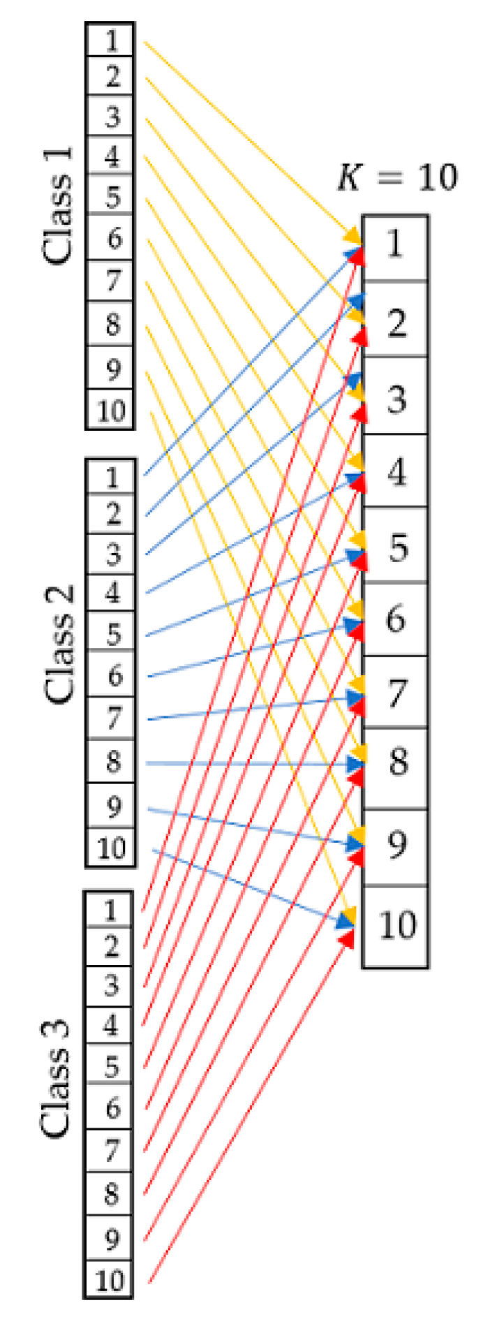
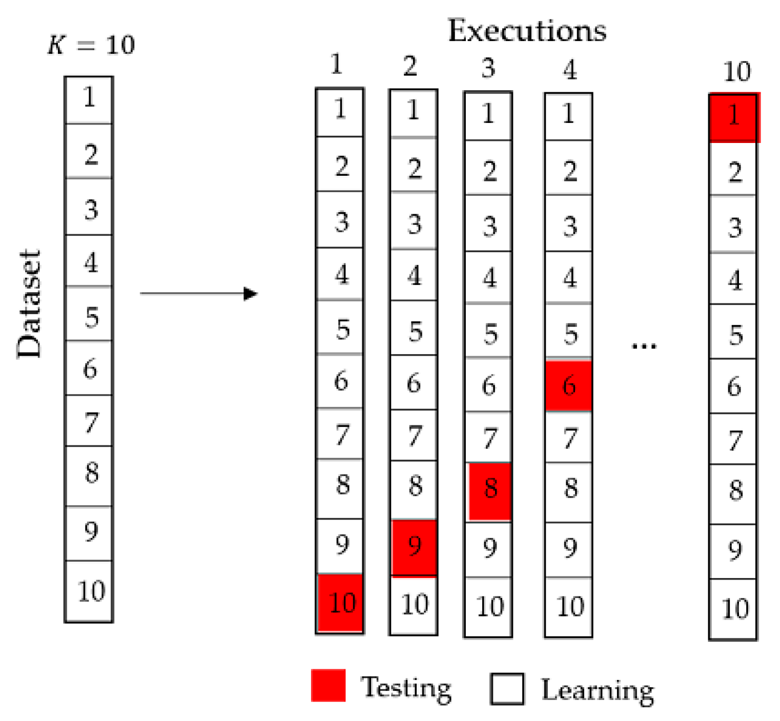
As the datasets were taken from three different repositories, with the exception of the datasets of the Keel repositories that provides the files under the 10-Fold cross validation method, a Python program of the algorithm of the 10-Fold cross validation method was developed as described in Figure 2 and Figure 3.

Once learn classes and test classes were generated, the Weka software was applied.

Table 4. Performance of the classifiers using Balanced Accuracy as a metric.

Dataset	MLP	NB	3-NN	C4.5	Logistic	DL	SVM
appendicitis	0.869	0.850	0.854	0.843	0.859	0.799	0.874
audiology	0.832	0.735	0.686	0.779	0.792	0.072	0.802
breast	0.701	0.744	0.751	0.769	0.715	0.731	0.681
BCWD2	0.958	0.926	0.968	0.931	0.946	0.978	0.979
Cleveland	0.532	0.566	0.555	0.525	0.597	0.560	0.443
contraceptive	0.532	0.496	0.456	0.530	0.508	0.504	0.512
dermatology	0.972	0.969	0.969	0.943	0.980	0.974	0.978
diabetes	0.754	0.763	0.727	0.738	0.772	0.773	0.771
E coli	0.655	0.810	0.807	0.795	0.777	0.732	0.635
Haberman	0.731	0.748	0.693	0.732	0.745	0.735	0.636
heart	0.804	0.852	0.770	0.781	0.841	0.854	0.837
heart	0.776	0.828	0.815	0.785	0.0820	0.824	0.828
heart failure	0.736	0.769	0.712	0.806	0.829	0.821	0.835
hepatitis	0.819	0.882	0.826	0.839	0.845	0.649	0.846
lymphography	0.798	0.817	0.806	0.743	0.738	0.789	0.866
mammographic	0.825	0.821	0.793	0.814	0.827	0.825	0.795
New thyroid	0.959	0.972	0.954	0.921	0.968	0.933	0.905
Pima	0.747	0.762	0.728	0.742	0.772	0.774	0.771
primary tumor	0.383	0.501	0.451	0.398	0.440	0.426	0.461
saheart	0.695	0.704	0.695	0.684	0.723	0.724	0.705
spect train	0.638	0.713	0.675	0.713	0.663	0.674	0.699
thyroid	0.968	0.954	0.939	0.996	0.959	0.950	0.848
Wisconsin	0.955	0.962	0.967	0.956	0.969	0.970	0.970
Total wins	2	7	0	3	3	5	6

shows the behavior of the classifiers according to Balanced Accuracy. Best results are highlighted in bold and indicate that a particular classifier performed better compared to the other classifiers.

As shown in Table 4, the classifiers with best performance according to Balanced Accuracy measure is Naïve Bayes with seven wins, followed by SVM and Deep Learning, with six and five wins, respectively.

However, the variation in the results is extremely high, ranging from 0.50 to 0.97 for Naïve Bayes, 0.072 to 0.97 for Deep Learning and 0.443 to 0.979 for SVM.

It should be noted at this stage of the research work that this heavy variation supports the need for establishing one of the most important contributions of the present paper: the a priori establishment of the performance of the classifiers, by means of meta-learning procedures.

Table 5. Performance of the classifiers using Sensitivity as a metric.

Dataset	MLP	NB	3-NN	C4.5	Logistic	DL	SVM
appendicitis	0.858	0.858	0.840	0.858	0.858	0.802	0.877
audiology	0.832	0.735	0.686	0.779	0.792	0.074	0.819
breast	0.690	0.755	0.747	0.755	0.697	0.733	0.693
BCWD2	0.958	0.926	0.968	0.931	0.946	0.979	0.979
Cleveland	0.525	0.549	0.562	0.485	0.593	0.562	0.582
contraceptive	0.545	0.493	0.445	0.532	0.516	0.508	0.510
dermatology	0.975	0.975	0.969	0.953	0.975	0.975	0.978
diabetes	0.754	0.763	0.727	0.738	0.772	0.775	0.773
E coli	0.810	0.789	0.821	0.798	0.795	0.735	0.780
Haberman	0.725	0.752	0.670	0.716	0.735	0.739	0.732
heart	0.822	0.837	0.774	0.774	0.837	0.855	0.837
heart	0.775	0.827	0.813	0.785	0.815	0.827	0.827
heart failure	0.736	0.769	0.712	0.806	0.829	0.823	0.836
hepatitis	0.813	0.875	0.825	0.863	0.813	0.650	0.850
lymphography	0.831	0.851	0.818	0.791	0.777	0.791	0.865
mammographic	0.806	0.824	0.771	0.840	0.827	0.827	0.792
new thyroid	0.944	0.967	0.935	0.921	0.958	0.935	0.898
Pima	0.760	0.755	0.735	0.743	0.776	0.775	0.773
primary tumor	0.383	0.501	0.451	0.398	0.440	0.428	0.469
saheart	0.669	0.716	0.675	0.708	0.725	0.725	0.710
spect train	0.638	0.731	0.675	0.713	0.663	0.675	0.700
thyroid	0.969	0.955	0.939	0.997	0.957	0.951	0.938
Wisconsin	0.963	0.962	0.966	0.959	0.965	0.971	0.969
Total wins	2	7	1	3	3	6	6

shows the behavior of the classifiers according to Sensitivity.

According to sensitivity (Table 5), the classifier with best performance is Naïve Bayes, with seven wins, followed by Deep Learning and SVM, with six wins.

However, as for Balanced Accuracy, the variation in the results is extremely high, ranging from 0.493 to 0.975 for Naïve Bayes, 0.51 to 0.979 for SVM, and 0.0743 to 0.979 for Deep Learning.

Table 6. Performance of the classifiers using Specificity as a metric.

Dataset	MLP	NB	3-NN	C4.5	Logistic	DL	SVM
appendicitis	0.848	0.852	0.836	0.850	0.852	0.796	0.870
audiology	0.826	0.728	0.681	0.772	0.789	0.069	0.786
breast	0.682	0.748	0.740	0.749	0.694	0.728	0.669
BCWD2	0.949	0.919	0.966	0.929	0.941	0.977	0.979
Cleveland	0.518	0.539	0.558	0.479	0.589	0.558	0.304
contraceptive	0.541	0.487	0.439	0.526	0.512	0.501	0.513
dermatology	0.973	0.969	0.963	0.949	0.974	0.974	0.978
diabetes	0.744	0.753	0.721	0.734	0.769	0.770	0.769
E coli	0.800	0.783	0.816	0.794	0.793	0.730	0.490
Haberman	0.720	0.745	0.665	0.710	0.731	0.730	0.540
heart	0.820	0.831	0.769	0.769	0.834	0.854	0.837
heart	0.770	0.821	0.808	0.780	0.810	0.822	0.828
heart failure	0.074	0.760	0.708	0.801	0.827	0.819	0.833
hepatitis	0.810	0.870	0.819	0.859	0.809	0.647	0.841
lymphography	0.823	0.799	0.813	0.786	0.770	0.787	0.867
mammographic	0.799	0.839	0.765	0.836	0.820	0.824	0.797
New thyroid	0.939	0.961	0.929	0.919	0.957	0.931	0.911
Pima	0.752	0.749	0.728	0.739	0.774	0.773	0.769
primary tumor	0.369	0.490	0.447	0.394	0.433	0.424	0.452
saheart	0.658	0.711	0.669	0.731	0.720	0.722	0.700
spect train	0.623	0.717	0.670	0.729	0.658	0.672	0.697
thyroid	0.965	0.950	0.932	0.996	0.954	0.949	0.758
Wisconsin	0.960	0.958	0.962	0.956	0.962	0.969	0.970
Total wins	3	5	1	4	2	2	6

shows the behavior of the classifiers according to Specificity.

According to specificity (Table 6), the classifier with best performance is SVM (six wins), followed by Naïve Bayes (five wins). It is interesting that Deep Learning showed poor behavior regarding specificity, with only two wins.

Again, the variation in the results is extremely high, ranging from 0.304 to 0.979 for SVM.

4.2. Statistical Analysis

Despite the previous results, which support the idea that the best performed classifiers are Naïve Bayes and Support Vector Machines, there is a need to establish if the differences in performance among the classifiers are significant or not. To do so, several authors suggest the use of non-parametric statistical tests [56].

For statistical analysis, we used the Friedman test for the comparison of multiple related samples [57] and the Holm test for post hoc analysis [58]. The application of the Friedman test implies the creation of a block for each of the samples analyzed in such a way that each block contains an observation from the application of each of the different contrasts or treatments. In terms of matrices, the blocks correspond to rows and the treatments to columns.

The null hypothesis establishes that the performances obtained by different treatments are equivalent, while the alternative hypothesis proposes that there is a difference between these performances, which would imply differences in the central tendency.

If k is defined as the number of treatments, then for each block a range between 1 and k is assigned to each input, 1 to the best result and k to the worst. In case of ties, the average rank is assigned. Next, the variable R_j (j = 1,…, k) is assigned the value of the sum of the ranges corresponding to each treatment. If the performances obtained from the different treatments are equivalent, then R_j = R_j for all i ≠ j. Thus, from this procedure it is possible to determine when an observed disparity between the R_j is sufficient to reject the null hypothesis. Let n be the number of blocks, and k be the number of treatments, then the Friedman statistic (S) is given by:

$$S=\frac{12}{nk\left(k+1\right)}\left[{\displaystyle \sum }_{j=1}^k{R}_j^2\right]-3n\left(k+1\right)$$

(7)

For values of n ≥ 10 and k ≥ 4, the S statistic approximates a chi-square random variable with k − 1 degrees of freedom. The critical region of size $\alpha$ is the right tail of the distribution of said variable. The null hypothesis is rejected when the value of S is greater than the critical value.

In the case that the Friedman test determines the existence of significant differences in the performance of the algorithms, it is recommended to use a post hoc test to determine between which of the algorithms compared in the Friedman test there are such differences. Holm’s post hoc test is designed to reduce type I errors when analyzing phenomena that include several hypotheses, and consists of adjusting the rejection criterion for each one of them.

The procedure begins with the ascending ordering of the probability values of each hypothesis. Once ordered, each of these values is compared with the quotient obtained by dividing the level of significance by the total number of hypotheses whose p-value has not been compared. When finding some p-value that exceeds this quotient, all the null hypotheses associated with the p-values that have already been compared are rejected.

Let $H1,\dots , Hk$ be a group of k hypotheses and $p1,\dots , pk$ the corresponding probability values. By ordering these p-values in ascending order, a new nomenclature is established: $p\left(1\right), p\left(2\right),\dots , p\left(k\right)$ for the ordered p-values and $H\left(1\right), H\left(2\right),\dots , H\left(k\right)$ for the hypothesis associated with each of them. If $\alpha$ is the level of significance and j is the minimum index for which it is satisfied that $p_{\left(j\right)}>\frac{\alpha }{k-j+1}$ then the null hypotheses $H\left(1\right), \dots , H\left(j-1\right)$ are rejected.

For both Friedman and Holm test, a significance level $\alpha$ = 0.05 was established, for 95% confidence. We begin by establishing the following hypotheses:

H0: 

There are no significant differences in the performance of the algorithms.

H1: 

There are significant differences in the performance of the algorithms.

The Friedman test obtained a significance values of 0.01758, 0.017996 and 0.152972, for Balanced Accuracy, Sensitivity and Specificity measures, respectively. Therefore, the null hypothesis for both Balanced Accuracy and Sensitivity measures are rejected, showing that there are significant differences in the performance of the compared algorithms.

Table 7. Ranking obtained by the Friedman test.

Algorithm	Balanced Accuracy Ranking	Sensitivity Ranking	Specificity Ranking
Multilayer Perceptron (MLP)	4.6087	4.5435	4.4783
Naïve Bayes (NB)	3.2391	3.4565	3.6087
3-NN	4.9130	5.0870	4.9130
C4.5	4.7174	4.5217	4.3043
Logistic regression (Logistic)	3.2609	3.4565	3.4565
Deep Learning (DL)	3.6522	3.7826	3.6957
Support Vector Machines (SVM)	3.6087	3.1522	3.5435

shows the ranking obtained by the Friedman test.

As can be seen in Table 7, the first algorithm in the ranking for Balanced Accuracy was Naïve Bayes, for Sensitivity this was SVM, and for Specificity the best algorithm was Logistic. Holm’s test compares the performance of the best ranked algorithm with the remaining ones.

Table 8. Holm’s post hoc test for Balanced Accuracy.

i	Algorithm	z	p	$\mathbf{Holm} (\mathit{\alpha }/\mathit{i})$
6	3-NN	2.627716	0.008596	0.008333
5	C4.5	2.32058	0.02031	0.010000
4	MLP	2.149949	0.031559	0.012500
3	DL	0.648397	0.516728	0.016667
2	SVM	0.580145	0.561817	0.025000
1	Logistic	0.034126	0.972777	0.050000

shows the results of the Holm’s test for Balanced Accuracy.

Table 9. Holm’s post hoc test for Sensitivity.

i	Algorithm	z	p	$\mathbf{Holm} (\mathit{\alpha }/\mathit{i})$
6	3NN	3.03723	0.002388	0.008333
5	MLP	2.184076	0.028957	0.010000
4	C4.5	2.149949	0.031559	0.012500
3	DL	0.989659	0.322341	0.016667
2	NB	0.477767	0.632816	0.025000
1	Logistic	0.477767	0.632816	0.050000

shows the results of the Holm’s test for Sensitivity.

For Balanced Accuracy, Holm’s procedure rejects the hypotheses that have an unadjusted p-value ≤ 0.01. The results of the Holm test show that there are no significant differences in the performance of the Naïve Bayes algorithm with respect to the compared algorithms apart from 3-NN, which showed a significantly worse behavior according to Balanced Accuracy.

For Sensitivity, in addition to 3-NN, which maintained a significantly worse behavior, the Multilayer Perceptron algorithm was also significantly worse than the SVM classifier.

4.3. Meta-Learning

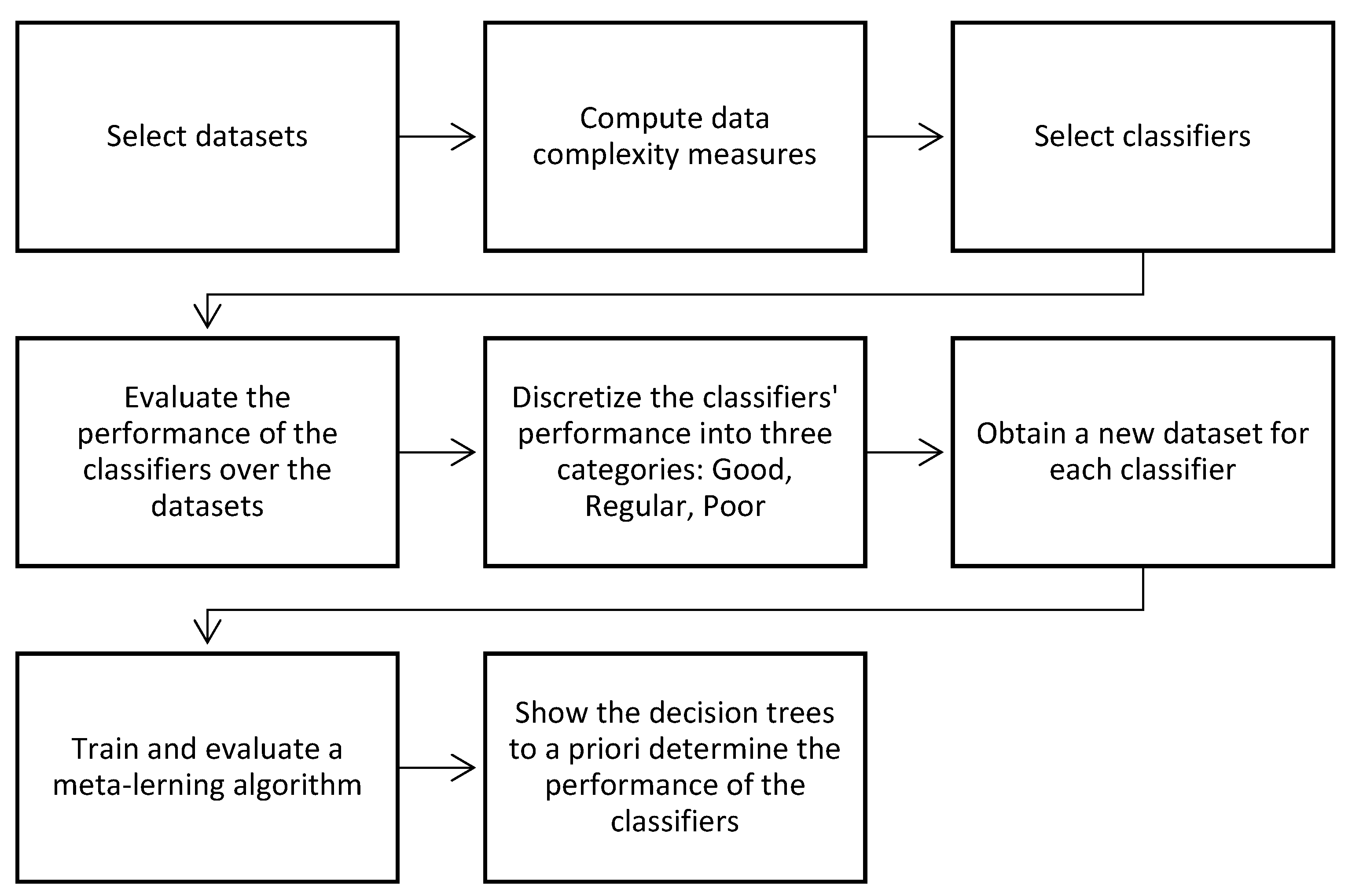
After obtaining the results for the compared classifiers, we discretized the performance values into three categories of performance: Good, Regular and Poor. Then, for each classifier, we obtained a new dataset, having as conditional attributes the values of the 12 complexity measures of Table 2, and as decision (class) attribute the discretized performance.

We used the Balanced Accuracy measure as decision attribute, due to the fact that it integrates the results of both sensitivity and specificity.

With such information, we were able to train a decision tree to a priori determine the performance of the classifiers. The decision tree is shown in Figure 4.

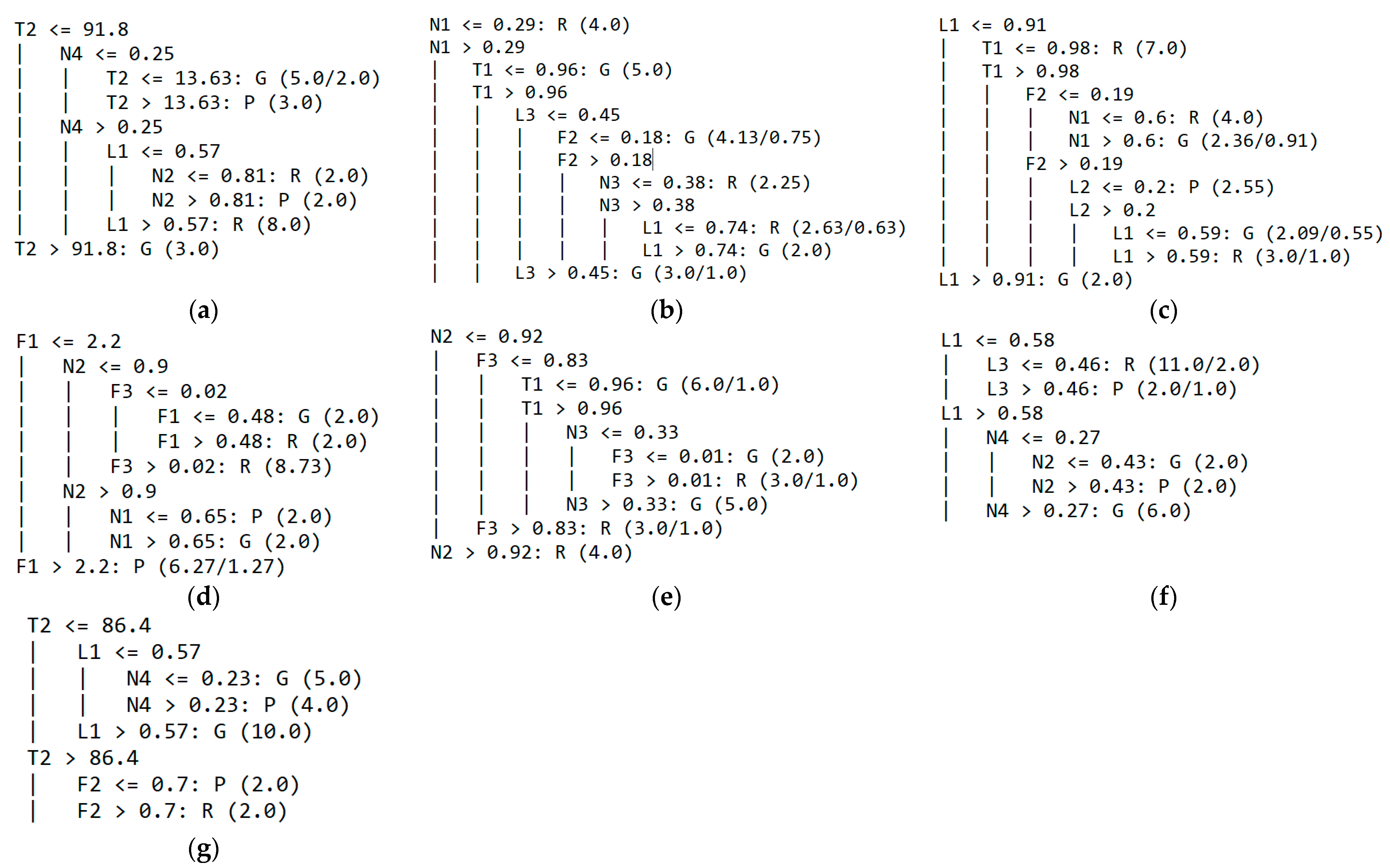
In the following, we show the performance results of our proposed meta-learning decision tree (in the form of a confusion matrix), as well as the obtained tree, for each classifier. In the decision trees, G stands for Good, P for Poor and R for Regular.

For the MLP classifier, the proposed meta-learning algorithm had only two errors: a dataset with Regular performance and a dataset with Poor performance, both classified as having Good performance, for a Balanced Accuracy of 0.9144.

The corresponding confusion matrix is shown in

Table 10. Confusion matrix of the proposed meta-learning for the MLP classifier.

		Predicted Class
		Good	Regular	Poor
True class	Good	6	0	0
	Regular	1	10	0
	Poor	1	0	5

.

The resulting decision tree (Figure 4a) has only six leaves, with size = 11. The decision tree only considers complexity measures L1, N2, N4 and T2 to make the decision.

As for the MLP classifier, the proposed meta-learning algorithm had only two errors (

Table 11. Confusion matrix of the proposed meta-learning for the Naïve Bayes classifier.

		Predicted Class
		Good	Regular	Poor
True class	Good	12	0	1
	Regular	1	9	0
	Poor	0	0	0

): a dataset with Regular performance and a dataset with Poor performance, both classified as having Good performance, for a Balanced Accuracy of 0.6410.

The dataset with Poor performance, assigned to have a Good performance, was the BCWD2, in which the classifier obtained the last place, with 0.9261 Balanced Accuracy, which was not a bad result per se.

The resulting decision tree (Figure 4b) has only seven leaves, with size = 13. The decision tree only considers complexity measures F2, L3, N1, N3 and T1 to make the decision.

For the 3-NN classifier, the proposed meta-learning algorithm had again only two errors: a dataset with Regular performance predicted as having Poor performance and a dataset with Poor performance classified as having Regular performance, for a Balanced Accuracy of 0.8929, as shown in

Table 12. Confusion matrix of the proposed meta-learning for the 3-NN classifier.

		Predicted Class
		Good	Regular	Poor
True class	Good	5	0	0
	Regular	0	13	1
	Poor	0	1	3

.

The resulting decision tree (Figure 4c) has only seven leaves, with size = 13. The decision tree only considers complexity measures F2, L1, L2, N1, and T1 to make the decision. For the C4.5 classifier, the proposed meta-learning algorithm had only one error (

Table 13. Confusion matrix of the proposed meta-learning for the C4.5 classifier.

		Predicted Class
		Good	Regular	Poor
True class	Good	4	0	1
	Regular	0	11	0
	Poor	0	0	7

): a dataset with Good performance predicted as having Poor performance, for a Balanced Accuracy of 0.9333.

The resulting decision tree (Figure 4d) has only six leaves, with size = 11. The decision tree only considers complexity measures F1, F3, N1, and N2 to make the decision.

For the Logistic classifier, the proposed meta-learning algorithm did not have good results. It misclassified the two datasets with Poor performance, assigning them into Regular and Good classes.

In addition, it misclassified a dataset with Good performance, and predicted it as Regular (

Table 14. Confusion matrix of the proposed meta-learning for the Logistic classifier.

		Predicted Class
		Good	Regular	Poor
True class	Good	12	1	0
	Regular	0	8	0
	Poor	1	1	0

); such results correspond to a Balanced Accuracy of 0.5744. The resulting decision tree (Figure 4e) again has six leaves, for a tree size of 11, and includes only the measures N2, N3, F3 and T1 of data complexity.

For the Deep Learning classifier, the proposed meta-learning algorithm misclassified the three datasets (two of them with Good performance, assigned into Regular and Bad classes, and another of Poor performance, assigned into Regular class).

The corresponding confusion matrix is shown in

Table 15. Confusion matrix of the proposed meta-learning for the Deep Learning classifier.

		Predicted Class
		Good	Regular	Poor
True class	Good	8	1	1
	Regular	0	9	0
	Poor	0	1	3

, with a Balanced Accuracy of 0.8561.

The resulting decision tree (Figure 4f) is quite small, with only five leaves for a tree size of nine, and it includes only the measures L1, L2, N2 and N4 of data complexity.

Last but not least, for the Support Vector Machine classifier (one of the best-performing algorithms for medical datasets), the proposed meta-learning decision tree was the best, with all datasets correctly classified, for a perfect Balanced Accuracy of 1.0. Such results were obtained with a very small decision tree (Figure 4g), of five leaves and tree size of nine, using only three complexity measures: L1, F2 and T2.

In our opinion, such results represent a breakthrough for medical datasets classification, because they allow determination a priori of the expected performance of the seven analyzed classifiers, six of them with Balanced Accuracy over 0.85, which is very promising.

5. Conclusions

After having selected a considerable number of datasets from the main available repositories, the authors of this paper evaluated the performance of some of the most relevant classifiers in state of the art machine learning and related areas.

However, the scope of the proposal was not limited to calculating the Sensitivity, Specificity and Balanced Accuracy values, but also performed a statistical analysis, with the support of the Friedman and Holm statistical tests.

One of the main contributions was a meta-learning process, whose usefulness to medical teams is undeniable. From the results of this paper, teams of doctors and human health researchers will have a valuable tool that can support them in making decisions about which classifier, or group of classifiers, could help them in pre-diagnoses of specific diseases.

A generic conclusion points out that the SVM model is one of the best-performing algorithms for medical datasets. This is based on facts such as the case of a perfect Balanced Accuracy of 1.0 in the decision tree during the meta-learning process. Such results were obtained with a very small decision tree of five leaves, using only three complexity measures: L1, F2 and T2. In our opinion, such results represent a breakthrough for medical dataset classification, due to the determination a priori of the expected performance of the seven analyzed classifiers, which could be a valuable aid to medical teams.

As future work, we plan to include more existing datasets in medical disease repositories and include classification algorithms such as convolutional neural networks, associative classifiers, and deep learning algorithm, seeking to obtain data sets of diseases that are of interest in hospitals to test the performance of the classifiers studied, with regard to current needs.

References

1. Burkart, N.; Huber, M.F. A survey on the explainability of supervised machine learning. J. Artif. Intell. Res. 2021, 70, 245–317. [Google Scholar] [CrossRef]
2. Duda, R.O.; Hart, P.E.; Stork, D.G. Pattern Classification, 2nd ed.; John Wiley & Sons: New York, NY, USA, 2001; pp. 20–450. [Google Scholar]
3. Wolpert, D.H.; Macready, W.G. No free lunch theorems for optimization. IEEE Trans. Evol. Comput. 1997, 1, 67–82. [Google Scholar] [CrossRef] [Green Version]
4. Adam, S.P.; Alexandropoulos, S.A.N.; Pardalos, P.M.; Vrahatis, M.N. No free lunch theorem: A review. In Approximation and Optimization; Demetriou, I., Pardalos, P., Eds.; Springer: Cham, Switzerland, 2019; Volume 145, pp. 57–82. [Google Scholar]
5. Ruan, S.; Li, H.; Li, C.; Song, K. Class-Specific Deep Feature Weighting for Naïve Bayes Text Classifiers. IEEE Access 2020, 8, 20151–20159. [Google Scholar] [CrossRef]
6. Paranjape, P.; Dhabu, M.; Deshpande, P. A novel classifier for multivariate instance using graph class signatures. Front. Comput. Sci. 2020, 14, 144307. [Google Scholar] [CrossRef]
7. Guan, Q.; Huang, Y.; Zhong, Z.; Zheng, Z.; Zheng, L.; Yang, Y. Thorax disease classification with attention guided convolutional neural network. Pattern Recognit. Lett. 2020, 131, 38–45. [Google Scholar] [CrossRef]
8. Dua, D.; Taniskidou, E.K. UCI Machine Learning Repository; University of California, School of Information and Computer Science: Irvine, CA, USA, 2017; Available online: http://archive.ics.uci.edu/ml (accessed on 5 May 2021).
9. Alcalá-Fdez, J.; Fernández, A.; Luengo, J.; Derrac, J.; García, S.; Sánchez, L.; Herrera, F. Keel data-mining software tool: Data set repository, integration of algorithms and experimental analysis framework. J. Mult.-Valued Log. Soft Comput. 2011, 17, 255–287. [Google Scholar]
10. Fernández, A.; López, V.; Galar, M.; del Jesus, M.J.; Herrera, F. Analysing the classification of unbalanced data-sets with multiple classes: Binarization techniques and ad-hoc approaches. Knowl.-Based Syst. 2013, 42, 97–110. [Google Scholar] [CrossRef]
11. Mullick, S.S.; Datta, S.; Dhekane, S.G.; Das, S. Appropriateness of performance indices for imbalanced data classification: An analysis. Pattern Recognit. 2020, 102, 107197. [Google Scholar] [CrossRef]
12. Hall, M.; Frank, E.; Holmes, G.; Pfahringer, B.; Reutemann, P.; Witten, I.H. The WEKA data mining software: An update. ACM SIGKDD Explor. Newsl. 2009, 11, 10–18. [Google Scholar] [CrossRef]
13. Triguero, I.; González, S.; Moyano, J.M.; García López, S.; Alcalá Fernández, J.; Luengo, J.; Fernández, A.; del Jesús, M.J.; Sánchez, L.; Herrera, F. KEEL 3.0: An open source software for multi-stage analysis in data mining. Int. J. Comput. Intell. Syst. 2017, 10, 1238–1249. [Google Scholar] [CrossRef] [Green Version]
14. Zhang, S. Cost-sensitive KNN classification. Neurocomputing 2020, 391, 234–242. [Google Scholar] [CrossRef]
15. Zhao, Z.; Xu, S.; Kang, B.H.; Kabir, M.M.J.; Liu, Y.; Wasinger, R. Investigation and improvement of multi-layer perceptron neural networks for credit scoring. Expert Syst. Appl. 2015, 42, 3508–3516. [Google Scholar] [CrossRef]
16. Livieris, I.E.; Kanavos, A.; Tampakas, V.; Pintelas, P. An Ensemble SSL Algorithm for Efficient Chest X-Ray Image Classification. J. Imaging 2018, 4, 95. [Google Scholar] [CrossRef] [Green Version]
17. Minaee, S.; Yao, W.; Lui, Y.W. Prediction of Longterm Outcome of Neuropsychological Tests of MTBI Patients Using Imaging Features. In Proceedings of the 2013 IEEE Signal Processing in Medicine and Biology Symposium (SPMB), Brooklyn, NY, USA, 7 December 2013; pp. 1–6. [Google Scholar]
18. Chan, H.-P.; Hadjiiski, L.M.; Samala, R.K. Computer-Aided Diagnosis in the Era of Deep Learning. Med. Phys. 2020, 47, e218–e227. [Google Scholar] [CrossRef] [PubMed]
19. Pathan, S.; Kumar, P.; Pai, R.M.; Bhandary, S.V. Automated Segmentation and Classifcation of Retinal Features for Glaucoma Diagnosis. Biomed. Signal Process. Control 2021, 63. [Google Scholar] [CrossRef]
20. Gautam, A.; Raman, B. Towards Effective Classification of Brain Hemorrhagic and Ischemic Stroke Using CNN. Biomed. Signal Process. Control 2021, 63. [Google Scholar] [CrossRef]
21. Mbarki, W.; Bouchouicha, M.; Frizzi, S.; Tshibasu, F.; Farhat, L.B.; Sayadi, M. Lumbar Spine Discs Classification Based on Deep Convolutional Neural Networks Using Axial View MRI. Interdiscip. Neurosurg. Adv. Tech. Case Manag. 2020, 22. [Google Scholar] [CrossRef]
22. Martínez-Más, J.; Bueno-Crespo, A.; Martínez-España, R.; Remezal-Solano, M.; Ortiz-González, A.; Ortiz-Reina, S.; Martínez-Cendán, J.P. Classifying Papanicolaou Cervical Smears through a Cell Merger Approach by Deep Learning Technique. Expert Syst. Appl. 2020, 160. [Google Scholar] [CrossRef]
23. Zhou, H.; Wang, K.; Tian, J. Online Transfer Learning for Differential Diagnosis of Benign and Malignant Thyroid Nodules with Ultrasound Images. IEEE Trans. Biomed. Eng. 2020, 67, 2773–2780. [Google Scholar] [CrossRef]
24. Reyes-León, P.; Salgado-Ramírez, J.C.; Velázquez-Rodríguez, J.L. Application of the Lernmatrix tau[9] to the classification of patterns in medical datasets. Int. J. Adv. Trends Comput. Sci. Eng. 2020, 9. [Google Scholar] [CrossRef]
25. Ding, W.; Nayak, J.; Swapnarekha, H.; Abraham, A.; Naik, B.; Pelusi, D. Fusion of intelligent learning for COVID-19: A state-of-the-art review and analysis on real medical data. Neurocomputing 2021, 457, 40–66. [Google Scholar] [CrossRef] [PubMed]
26. Yu, X.; Lu, S.; Guo, L.; Wang, S.-H.; Zhang, Y.-D. ResGNet-C: A graph convolutional neural network for detection of COVID-19. Neurocomputing 2021, 452, 592–605. [Google Scholar] [CrossRef]
27. Xu, Y.; Lam, H.-K.; Jia, G. MANet: A two-stage deep learning method for classification of COVID-19 from Chest X-ray images. Neurocomputing 2021, 443, 96–105. [Google Scholar] [CrossRef] [PubMed]
28. Luján-García, J.E.; Moreno-Ibarra, M.A.; Villuendas-Rey, Y.; Yáñez-Márquez, C. Fast COVID-19 and Pneumonia Classification Using Chest X-Ray Images. Mathematics 2020, 8, 1423. [Google Scholar] [CrossRef]
29. Yazdani, S.; Minaee, S.; Kafieh, R.; Saeedizadeh, N.; Sonka, M. COVID CT-Net: Predicting Covid-19 From Chest CT Images Using Attentional Convolutional Network. arXiv 2020, arXiv:2009.05096. [Google Scholar]
30. Gupta, A.; Gupta, S.; Katarya, R. InstaCovNet-19: A Deep Learning Classification Model for the Detection of COVID-19 Patients Using Chest X-Ray. Appl. Soft Comput. 2021, 99, 106859. [Google Scholar] [CrossRef]
31. Dias Júnior, D.A.; da Cruz, L.B.; Bandeira Diniz, J.O.; França da Silva, G.L.; Junior, G.B.; Silva, A.C.; de Paiva, A.C.; Nunes, R.A.; Gattass, M. Automatic method for classifying COVID-19 patients based on chest X-ray images, using deep features and PSO-optimized XGBoost. Expert Syst. Appl. 2021, 183, 115452. [Google Scholar] [CrossRef]
32. Rangarajan, A.K.; Ramachandran, H.K. A preliminary analysis of AI based smartphone application for diagnosis of COVID-19 using chest X-ray images. Expert Syst. Appl. 2021, 183, 115401. [Google Scholar] [CrossRef]
33. da Silva, T.T.; Francisquini, R.; Nascimento, M.C.V. Meteorological and human mobility data on predicting COVID-19 cases by a novel hybrid decomposition method with anomaly detection analysis: A case study in the capitals of Brazil. Expert Syst. Appl. 2021, 182, 115190. [Google Scholar] [CrossRef]
34. Alhudhaif, A.; Polat, K.; Karaman, O. Determination of COVID-19 pneumonia based on generalized convolutional neural network model from chest X-ray images. Expert Syst. Appl. 2021, 180, 115141. [Google Scholar] [CrossRef]
35. Pasa, F.; Golkov, V.; Pfeiffer, F.; Cremers, D.; Pfeiffer, D. Efficient Deep Network Architectures for Fast Chest X-Ray Tuberculosis Screening and Visualization. Sci. Rep. 2019, 9, 6268. [Google Scholar] [CrossRef] [Green Version]
36. Khatibi, T.; Shahsavari, A.; Farahani, A. Proposing a Novel Multi-Instance Learning Model for Tuberculosis Recognition from Chest X-Ray Images Based on CNNs, Complex Networks and Stacked Ensemble. Phys. Eng. Sci. Med. 2021, 44. [Google Scholar] [CrossRef]
37. Shen, L.; Margolies, L.R.; Rothstein, J.H.; Fluder, E.; McBride, R.; Sieh, W. Deep Learning to Improve Breast Cancer Detection on Screening Mammography. Sci. Rep. 2019, 9. [Google Scholar] [CrossRef] [PubMed]
38. Agarwal, R.; Diaz, O.; Lladó, X.; Hoon Yap, M.; Martí, R.; Agarwal, R. Automatic Mass Detection in Mammograms Using Deep Convolutional Neural Networks. J. Med. Imaging 2019, 6, 031409. [Google Scholar] [CrossRef]
39. Wu, N.; Phang, J.; Park, J.; Shen, Y.; Huang, Z.; Zorin, M.; Jastrzebski, S.; Fevry, T.; Katsnelson, J.; Kim, E.; et al. Deep Neural Networks Improve Radiologists’ Performance in Breast Cancer Screening. IEEE Trans. Med. Imaging 2020, 39, 1184–1194. [Google Scholar] [CrossRef] [PubMed] [Green Version]
40. Lindberg, A. Developing Theory Through Integrating Human and Machine Pattern Recognition. J. Assoc. Inf. Syst. 2020, 21, 7. [Google Scholar] [CrossRef]
41. Daqi, G.; Yan, J. Classification methodologies of multilayer perceptrons with sigmoid activation functions. Pattern Recognit. 2005, 38, 1469–1482. [Google Scholar] [CrossRef]
42. Quinlan, J.R. Improved use of continuous attributes in C4. 5. J. Artif. Intell. Res. 1996, 4, 77–90. [Google Scholar] [CrossRef] [Green Version]
43. Quinlan, J.R. Induction of decision trees. Mach. Learn. 1986, 1, 81–106. [Google Scholar] [CrossRef] [Green Version]
44. Otneim, H.; Jullum, M.; Tjøstheim, D. Pairwise local Fisher and Naïve Bayes: Improving two standard discriminants. J. Econom. 2020, 216, 284–304. [Google Scholar] [CrossRef]
45. Cover, T.; Hart, P. Nearest neighbor pattern classification. IEEE Trans. Inf. Theory 1967, 13, 21–27. [Google Scholar] [CrossRef]
46. Yamashita, Y.; Wakahara, T. Affine-transformation and 2D-projection invariant k-NN classification of handwritten characters via a new matching measure. Pattern Recognit. 2016, 52, 459–470. [Google Scholar] [CrossRef]
47. Noh, Y.-K.; Zhang, B.-T.; Lee, D.D. Generative Local Metric Learning for Nearest Neighbor Classification. IEEE Trans. Pattern Anal. Mach. Intell. 2018, 40, 106–118. [Google Scholar] [CrossRef] [PubMed]
48. Stoklasa, R.; Majtner, T.; Svoboda, D. Efficient k-NN based HEp-2 cells classifier. Pattern Recognit. 2014, 47, 2409–2418. [Google Scholar] [CrossRef]
49. Pernkopf, F. Bayesian network classifiers versus selective k-NN classifier. Pattern Recognit. 2005, 38, 1–10. [Google Scholar] [CrossRef]
50. le Cessie, S.; van Houwelingen, J.C. Ridge Estimators in Logistic Regression. Appl. Stat. 1992, 41, 191–201. [Google Scholar] [CrossRef]
51. Ho, T.K.; Basu, M. Complexity measures of supervised classification problems. IEEE Trans. Pattern Anal. Mach. Intell. 2002, 24, 289–300. [Google Scholar]
52. Schwenker, F.; Trentin, E. Pattern classification and clustering: A review of partially supervised learning approaches. Pattern Recognit. Lett. 2014, 37, 4–14. [Google Scholar] [CrossRef]
53. Stock, M.; Pahikkala, T.; Airola, A.; Waegeman, W.; De Baets, B. Algebraic shortcuts for leave-one-out cross-validation in supervised network inference. Brief. Bioinform. 2020, 21, 262–271. [Google Scholar] [CrossRef] [Green Version]
54. Jiang, G.; Wang, W. Error estimation based on variance analysis of k-fold cross-validation. Pattern Recognit. 2017, 69, 94–106. [Google Scholar] [CrossRef]
55. Soleymani, R.; Granger, E.; Fumera, G. F-measure curves: A tool to visualize classifier performance under imbalance. Pattern Recognit. 2020, 100, 107146. [Google Scholar] [CrossRef]
56. Garcia, S.; Herrera, F. An extension on statistical comparisons of classifiers over multiple data sets for all pairwise comparisons. J. Mach. Learn. Res. 2008, 9, 2677–2694. [Google Scholar]
57. Friedman, M. The Use of Ranks to Avoid the Assumption of Normality Implicit in the Analysis of Variance. J. Am. Stat. Assoc. 1937, 32, 675–701. [Google Scholar] [CrossRef]
58. Holm, S. A Simple Sequentially Rejective Multiple Test Procedure. Scand. J. Stat. 1979, 6, 65–70. [Google Scholar]
Figure 1. Schematic diagram of the experimental setup.
Mathematics 09 01817 g001
Figure 2. The 10-fold stratified cross validation method.
Mathematics 09 01817 g002
Figure 3. Operation of the 10-fold stratified cross validation method.
Mathematics 09 01817 g003
Figure 4. Decision trees for the classifiers. (a) MLP, (b) Naïve Bayes, (c) 3-NN, (d) C4.5, (e) Logistic, (f) Deep Learning and (g) SVM.
Mathematics 09 01817 g004