Evolutionary Games and Dynamics in Public Goods Supply with Repetitive Actions

Abstract

Based on a tripartite game model among suppliers of public goods, consumers, and the government, a tripartite repeated game model is constructed to analyze the evolution mechanism of which suppliers supply at low prices, consumers purchase, and the government provides incentives, and to establish the dynamics system of a repeated game. The equilibrium points of the evolutionary game are solved, and among them, the equilibrium points are found to satisfy the parameter conditions of ESS. The numerical simulation is employed to verify the impact of penalty coefficients and discount factors on the stability of strategies, which are adopted by the three players in a tripartite repeated game on public goods, and scenario analyses are conducted. The research results of this paper could provide a reference for the government, suppliers, and consumers to make rapid decisions, who are in the supply chain of public goods, especially quasi-public goods, such as coal, water, electricity, and gas, and help them to obtain stable incomes and then ensure the stable operation of the market.

1. Introduction

Evolutionary game theory, combining game theory with the basic theories of a dynamics system, is usually used to examine complex dynamic population issues. It has emerged as the most rapidly developing interdisciplinary subject in recent years. Inspired by biological evolution, Maynard Smith and Price (1973) introduced the idea of evolution in biological theory into game theory. In 1973, they published the seminal paper, The Logic of Animal Conflict [1], where they put forward the idea of evolutionary game and the concept of an evolutionary stability strategy [2] which marked the formal formation of evolutionary game theory. In 1978, ecologists Taylor and Jonker [3] carried out a series of studies using the replicative dynamic equations. In 1992, Cornell University held a conference on the development of game theory, which marked the establishment of the academic status of evolutionary game theory.

In 1954, American economist Samuelson pointed out in The Pure Theory of Public Expenditure that a public good is a kind of product. It refers to a product and labor service that can be shared by many at the same time. Public good is non-competitive in consumption or use and non-exclusive in benefit. It can be divided into pure public good and quasi-public good according to the nature. The scope of pure public goods is relatively narrow, such as the property and services of national defense, public security and justice, and so forth. However, the scope of quasi-public goods is relatively wide, such as education, culture, radio, television, hospitals, and so on, provided by public institutions to the society. In addition, the construction of infrastructure, such as water supply, power supply, post office, railway, port, wharf, and public transportation, which are subject to enterprise accounting, also falls within the scope of quasi-public goods.

The supply mechanism of public goods is a supply mode abstracted from the perspective of the supply body and the operating mechanism. Public goods can be provided by the public sector, private sector, or a combination of the two. Both Samuelson and Musgrave believed that public goods should be provided by the government because there must be a loss of efficiency or welfare in private supply. However, literature research [4] since then has shown the potential power of private sectors to provide lighthouses, education, law and order, infrastructure, and so on.

In the postdoctoral report, Fan Liming made a detailed analysis of the mechanism of government supply, market supply, and voluntary supply of public goods. He believed that the market supply mechanism of public goods is a mechanism for profit-making organizations to compensate expenses by charging fees according to the market demand and for profit purposes. Public goods enter the market for consumers to purchase. Enterprises provide public goods in the expectation of making social and economic benefits. The government, to preserve the public attributes of these goods, needs to resort to market intervention, which is to establish positive or negative incentives. Meanwhile, ordinary consumers need to consider the social attributes of public goods and choose whether to purchase them.

Repeated game, also called stage game, is a special type of dynamic games which is the repetition of the basic game. However, due to the constraints of future profits and long-term total incomes, the decision-making behavior and game results are often different from one-off games. In the late 1950s, game theorists began to study repeated games and obtained the Folk Theorem, which is related to repeated games. In 1976, Aumann and Shapley proposed to replace Nash equilibrium with subgame perfect equilibrium. Over the past few years, scholars have mainly studied the perfect equilibrium of infinitely repeated games without considering the discount factors. In 1971, Friedman proved that any Nash equilibrium outcomes in which Pareto dominates the original game can be established in a perfect equilibrium of repeated game [5]. In 1985, Abreu established a highly restricted set of strategies which can support any perfect equilibrium results. He proposes that whenever any participant deviates from the desired equilibrium path, no matter what the circumstances the game is in, other participants will turn to the worst possible equilibrium as punishment for deviants [6]. In 1986, in order to obtain the Folk Theorem in the extreme cases where the discount factor tends to be 1, Fudenberg and Maskin proposed: If the participants deviate from the equilibrium path, the other participants are encouraged to enact the minimum and maximum strategy on the deviators by means of incentives, rather than threatening them with a penalty [7].

So far, research on games of public goods have mainly focused on: theoretical analyses of market competitions based on Evolutionary Game between two or three, or even four groups [8,9], the innovation of synergetic mechanism based on three-group Evolutionary Game, and the mechanism coexistence or supply chain mechanism [10,11,12,13,14]. Yang, Yu, Yang, and Song et al. did a large amount of research on the equilibrium of population game [15,16,17,18,19,20,21,22]. Taking a multi-player repeated game in eBay online bidding as an example, Jin and Yu studied information asymmetry, reputation effect, and cooperation balance [23]; Laclaua and Tomala considered repeated games with public deterministic monitoring, compact action sets, and pure strategies [24]. Khakzad studied repeated games for eco-friendly flushing in reservoir study interactions between multiple self-interested parties (individuals or population) [25]. Escobara and Llanes studied cooperation dynamics in repeated games of adverse selection study cooperation dynamics in repeated games with Markovian private information [26]. However, there is a small number of papers which consider the long-term incomes of game players, especially in infinitely repeated games.

In this paper, a tripartite repeated game model and its evolutionary game model are constructed on the basis of existing literatures and related research. These new models are used to analyze the stability of equilibrium points of tripartite repeated evolutionary games in different situations, innovatively introducing the penalty coefficient and discount factors to the profit of suppliers and the government in the game. A numerical simulation is employed to verify the impact of penalty coefficients and discount factors on the stability of strategies adopted by the three players in the tripartite repeated game, and finally, a relatively comprehensive scenario analysis is carried out.

2. The Construction of Repeated Game Model

2.1. Tripartite Game Profit Model

In 2019, Premier Li Keqiang pointed out in the government report: “We will accelerate state capital and SOE (which is the abbreviation of State Owned Enterprises) reforms”. “Reforms will be deepened in sectors including power, oil and natural gas, and railways. In natural monopoly industries, network ownership and operation will be separated in light of the specific conditions of these industries to make the competitive aspects of their operations fully market-based”. “We will work for big improvements in the development environment for the private sector. We will uphold the ‘two no irresolutions’ principle, and encourage, support, and guide the development of the non-public sector. We will follow the principle of competitive neutrality, so that when it comes to access to factors of production, market access and licenses, business operations, government procurement, public biddings, and so on, enterprises under all forms of ownership will be treated on an equal footing”.

All of these mean that with the continuous deepening of China’s economic system reform and the reform of state-owned enterprises, the supply market for public goods is also facing severe competition. Therefore, it is of great significance to study the economic behavior of enterprises (suppliers), governments, and consumers in the supply of public goods in an environment of fierce market competition. A tripartite game model for the supply of public goods among suppliers (enterprises), the government, and consumers is constructed here based on the following assumptions.

Assumption 1.

When the supplier chooses low- or high-price supply strategies, the consumer adopts a purchasing strategy or non-purchase strategy, and the government takes an incentives or no incentives strategy, where the payoffs under the eight strategy combinations formed by the supplier, the consumer, and the government are as follows: $a,i,q$, $b,j,r$, $c,k,s$, $d,l,t$, $e,m,u$, $g,n,v$. $f,o,w$, $h,p$, $\Phi$. Naturally, all payoffs are non-negative.

Assumption 2.

The probabilities of suppliers choosing low-price strategies, consumers adopting purchasing strategies, and the government adopting incentive strategies are x, y, and z, respectively.

According to the assumption, the game income model of the three populations of suppliers, consumers, and the government is as shown in

Table 1. Tripartite game model.

Supplier	Consumer		Government
	Purchasing$(\mathit{y})$	Non-Purchasing$(1-\mathit{y})$
Low prices$(x)$	$a,i,q$	$b,j,r$	Incentive$(z)$
High price$(1-x)$	$c,k,s$	$d,l,t$
Low price$(x)$	$e,m,u$	$g,n,v$	Non-incentive$(1-z)$
High price$(1-x)$	$f,o,w$	$h,p,\Phi$

.

2.2. Strategy Choice of Repeated Players

When consumers choose purchasing strategies in the first game, the government and suppliers choose the following strategies:

After the first game, the government and the supplier have two options: the cooperation strategy of a betrayal strategy, which lead to discrepant choices later; the government and the supplier adopt cooperation strategies, either the government or the supplier adopts betrayal strategies, and both sides adopt betrayal strategies. These choices ultimately result in different profits. According to the analysis, there are the following four situations:

After the first game, both the government and the supplier choose to cooperate in the first round, and then continue to cooperate as long as the other side does not betray. In this case, the final cooperation profits of both sides are:

Supplier: ${\displaystyle a(1+\overline{\omega }+{\overline{\omega }}^2+{\overline{\omega }}^3+\cdots )=\frac{a}{1-\overline{\omega }}}$

Government: ${\displaystyle q(1+\overline{\omega }+{\overline{\omega }}^2+{\overline{\omega }}^3+\cdots )=\frac{q}{1-\overline{\omega }}}$.

After the first game, the government chooses to cooperate, and the supplier chooses to betray in the first round. Then, the government will always adopt betrayal strategies. Therefore, starting from the second round, the government chooses to betray and the supplier chooses to cooperate. In this case, the profits of the supplier who adopts betrayal strategies and the government who adopts a cooperation strategy are:

Supplier: ${\displaystyle c-\delta +(-\delta )(\overline{\omega }+{\overline{\omega }}^2+{\overline{\omega }}^3+\cdots )=\frac{(c-\delta )(1-\overline{\omega })-\delta \overline{\omega }}{1-\overline{\omega }}}$

Government: ${\displaystyle s+(-\delta )(\overline{\omega }+{\overline{\omega }}^2+{\overline{\omega }}^3+\cdots )=\frac{s(1-\overline{\omega })-\delta (\overline{\omega })}{1-\overline{\omega }}}$.

After the first game, the government chooses to betray and the supplier chooses to cooperate in the first round. Then the supplier will always adopt betrayal strategies. Therefore, starting from the second round, the government chooses to cooperate and the supplier chooses to betray. In this case, the profits of the supplier who adopts cooperation strategies and the government who adopts a betrayal strategy are:

Supplier: ${\displaystyle e+(-\delta )(\overline{\omega }+{\overline{\omega }}^2+{\overline{\omega }}^3+\cdots )=\frac{e(1-\overline{\omega })-\delta (\overline{\omega })}{1-\overline{\omega }}}$

Government: ${\displaystyle u-\delta +(-\delta )(\overline{\omega }+{\overline{\omega }}^2+{\overline{\omega }}^3+\cdots )=\frac{(u-\delta )(1-\overline{\omega })-\delta \overline{\omega }}{1-\overline{\omega }}}$.

After the first game, both the government and the supplier choose to betray in the first round. Then the government and the supplier will always adopt betrayal strategies. Therefore, starting from the second round, the government and the supplier choose to betray. In this case, the profits of the supplier and the government who adopt a betrayal strategy are:

Supplier: ${\displaystyle f+(-\delta )(1+\overline{\omega }+{\overline{\omega }}^2+{\overline{\omega }}^3+\cdots )=f+\frac{-\delta }{1-\overline{\omega }}}$

Government: ${\displaystyle w+(-\delta )(1+\overline{\omega }+{\overline{\omega }}^2+{\overline{\omega }}^3+\cdots )=w+\frac{-\delta }{1-\overline{\omega }}}$.

When consumers choose no purchase strategy and a purchase strategy in the first game, the strategy choices of the government and suppliers are similar. The revenues of the government and supplier are, respectively:

Supplier: ${\displaystyle \frac{b}{1-\overline{\omega }}}$, Government: ${\displaystyle \frac{r}{1-\overline{\omega }}}$.

Supplier: ${\displaystyle \frac{(d-\delta )(1-\overline{\omega })-\delta \overline{\omega }}{1-\overline{\omega }}}$, Government: ${\displaystyle \frac{t(1-\overline{\omega })-\delta (\overline{\omega })}{1-\overline{\omega }}}$.

Supplier: ${\displaystyle \frac{g(1-\overline{\omega })-\delta (\overline{\omega })}{1-\overline{\omega }}}$, Government: ${\displaystyle \frac{(v-\delta )(1-\overline{\omega })-\delta \overline{\omega }}{1-\overline{\omega }}}$.

Supplier: ${\displaystyle h+\frac{-\delta }{1-\overline{\omega }}}$, Government: ${\displaystyle \Phi +\frac{-\delta }{1-\overline{\omega }}}$.

2.3. Tripartite Repeated Game Model

The assumptions of the model are:

• $\delta (1>\delta >0)$ represents the penalty coefficient. Player of the game will be punished if he/she adopts a betrayal strategy (this article does not consider a $\delta$ execution cost).
• Discount factor $\overline{\omega }(1>\overline{\omega }>0)$ is the probability that the two sides will play in the next round of the game (the second stage of the game) after the first round is over. $1-\overline{\omega }$ is the probability of ending the game.
• In this repeated game, the cooperation or betrayal strategies of consumer are not taken into consideration.

According to Section 2.2 and the assumption, a tripartite repeated game model among suppliers, consumers, and the government is established, as shown in

Table 2. Tripartite repeated game model.

Supplier	Consumer		Government
	Purchasing$(\mathit{y})$	Non-Purchasing$(1-\mathit{y})$
Low prices$(x)$	$\frac{a}{1-\overline{\omega }},i,\frac{q}{1-\overline{\omega }}$	$\frac{b}{1-\overline{\omega }},j,\frac{r}{1-\overline{\omega }}$	Incentive$(z)$
High price$(1-x)$	$\frac{(c-\delta )(1-\overline{\omega })-\delta \overline{\omega }}{1-\overline{\omega }},k,\frac{s(1-\overline{\omega })-\delta \overline{\omega }}{1-\overline{\omega }}$	$\frac{(d-\delta )(1-\overline{\omega })-\delta \overline{\omega }}{1-\overline{\omega }},l,\frac{t(1-\overline{\omega })-\delta \overline{\omega }}{1-\overline{\omega }}$
Low price$(x)$	$\frac{e(1-\overline{\omega })-\delta \overline{\omega }}{1-\overline{\omega }},m,\frac{(u-\delta )(1-\overline{\omega })-\delta \overline{\omega }}{1-\overline{\omega }}$	$\frac{g(1-\overline{\omega })-\delta \overline{\omega }}{1-\overline{\omega }},n,\frac{(v-\delta )(1-\overline{\omega })-\delta \overline{\omega }}{1-\overline{\omega }}$	Non-incentive$(1-z)$
High price$(1-x)$	$f+\frac{-\delta }{1-\overline{\omega }},o,w+\frac{-\delta }{1-\overline{\omega }}$	$h+\frac{-\delta }{1-\overline{\omega }},p,\Phi +\frac{-\delta }{1-\overline{\omega }}$

.

3. Evolutionary Dynamics under Infinite Population

In a tripartite game among suppliers, consumers, and the government, assuming that their probability of adopting cooperation strategies are $x,y$, and z respectively, and thereby, the probabilities of adopting betrayal strategies are $1-x,1-y,1-z$. Hence, the profits of the supplier and the government who adopt different strategies can be obtained.

3.1. The Expected Profits of Suppliers, Consumers, and the Government

3.1.1. The Expected Profits of Suppliers

For suppliers, assuming that low-price supply is a cooperation strategy while high-price supply is a betrayal strategy, the expected profits $U_1^C,U_1^D$ are:

$$U_1^C=\frac{a}{1-\overline{\omega }}yz+\frac{b}{1-\overline{\omega }}(1-y)z+\frac{e(1-\overline{\omega })-\delta (\overline{\omega })}{1-\overline{\omega }}y(1-z)+\frac{g(1-\overline{\omega })-\delta (\overline{\omega })}{1-\overline{\omega }}(1-y)(1-z)$$

$$U_1^D=\frac{(c-\delta )(1-\overline{\omega })-\delta \overline{\omega }}{1-\overline{\omega }}yz+\frac{(d-\delta )(1-\overline{\omega })-\delta \overline{\omega }}{1-\overline{\omega }}(1-y)z+f+\frac{-\delta }{1-\overline{\omega }}y(1-z)+h+\frac{-\delta }{1-\overline{\omega }}(1-y)(1-z).$$

3.1.2. The Expected Profits of Consumers

For consumers, assuming that purchasing behavior is a cooperation strategy while non-purchasing behavior is a betrayal strategy, the expected profits $U_2^C,U_2^D$ are:

$$U_2^C=ixz+k(1-x)z+mx(1-z)+o(1-x)(1-z)$$

$$U_2^D=jxz+l(1-x)z+nx(1-z)+p(1-x)(1-z).$$

3.1.3. The Expected Profits of the Government

For the government, assuming that adopting incentives is a cooperation strategy while adopting non-incentives is a betrayal strategy, the expected benefits of $U_3^C,U_3^D$ are:

$$U_3^C=\frac{q}{1-\overline{\omega }}xy+\frac{r}{1-\overline{\omega }}x(1-y)+\frac{s(1-\overline{\omega })-\delta (\overline{\omega })}{1-\overline{\omega }}y(1-x)+\frac{t(1-\overline{\omega })-\delta (\overline{\omega })}{1-\overline{\omega }}(1-x)(1-y)$$

$$\begin{array}{c}{U}_3^D=\frac{(u-\delta )(1-\overline{\omega })-\delta \overline{\omega }}{1-\overline{\omega }}xy+\frac{(v-\delta )(1-\overline{\omega })-\delta \overline{\omega }}{1-\overline{\omega }}x(1-y)+(w+\frac{-\delta }{1-\overline{\omega }})(1-x)y\\ +(\Phi +\frac{-\delta }{1-\overline{\omega }})(1-x)(1-y).\end{array}$$

3.2. The Replicator Dynamic Equation of Repeated Game among Suppliers, Consumers, and the Government

According to the expected profits of suppliers, consumers, and the government, the replicator dynamic equation of a tripartite repeated game is obtained:

$$\begin{array}{c}{U}_1(x)=\frac{\mathit{d}x}{\mathit{d}t}=x(1-x)((e-g+f-h)y+[\frac{a-b+2\delta \overline{\omega }}{1-\overline{\omega }}+(g-e-c-d-f+h+2\delta )]yz\\ +[\frac{b-\delta }{1-\overline{\omega }}+(d-g-\delta +h)]z+g+\delta +h)\end{array}$$

$$\begin{array}{c}{U}_2(y)=\frac{\mathit{d}y}{\mathit{d}t}=y(1-y)[(m-o+n-p)x+(i-k-m+o-j-l-n+p)xz\\ +(k+l-o-p)z+o+p]\end{array}$$

$$\begin{array}{c}{U}_3(z)=\frac{dz}{dt}=z(1-z)([\frac{r+\delta }{1-\overline{\omega }}+(v-\delta -t-\Phi )]x+[\frac{q-r+2\delta \overline{\omega }}{1-\overline{\omega }}+\\ (t-s-u-v-w+\Phi +2\delta )]xy+(s-t+w-\Phi )y+t+\delta -\Phi ]\end{array}.$$

3.3. The Equilibrium Point of Evolutionary Process

According to the replicator dynamic equation of the tripartite repeated game, the following system can be set as:

$$\left\{\begin{array}{c}\frac{dx}{dt}=x(1-x)(U_1^C-U_1^D)\\ \frac{dy}{dt}=y(1-y)(U_2^C-U_2^D)\\ \frac{dz}{dt}=z(1-z)(U_3^C-U_3^D)\end{array}\right.$$

Let

${\alpha }_1=e-g+f-h,{\beta }_1=\frac{a-b+2\delta \overline{\omega }}{1-\overline{\omega }}+(g-e-c-d-f+h+2\delta ),{\theta }_1=\frac{b-\delta }{1-\overline{\omega }}+(d-g-\delta +h),{\eta }_1=g+\delta +h$

${\alpha }_2=m-o+n-p,{\beta }_2=i-k-m+o-j-l-n+p,{\theta }_2=k+l-o-p,{\eta }_2=o+p$

${\alpha }_3=\frac{r+\delta }{1-\overline{\omega }}+(v-\delta -t-\Phi ),{\beta }_3=[\frac{q-r+2\delta \overline{\omega }}{1-\overline{\omega }}+(t-s-u-v-w+\Phi +2\delta ),{\theta }_3=(s-t+w-\Phi ),{\eta }_3=t+\delta -\Phi$.

The system is converted into:

$$\left\{\begin{array}{c}\frac{dx}{dt}=x(1-x)({\alpha }_{1}y+{\beta }_{1}yz+{\theta }_{1}z+{\eta }_1)\\ \frac{dy}{dt}=y(1-y)({\alpha }_{2}x+{\beta }_{2}xz+{\theta }_{2}z+{\eta }_2)\\ \frac{dz}{dt}=z(1-z)({\alpha }_{3}x+{\beta }_{3}xy+{\theta }_{3}y+{\eta }_3)\end{array}\right.$$

(1)

For the three-dimensional dynamic system (1), let $\frac{dx}{dt}=0,\frac{dy}{dt}=0,\frac{dz}{dt}=0$, and the following theorems can be drawn:

Theorem 1.

The three-dimensional dynamic system (1) contains eight tripartite groups which all adopt equilibrium points featured by pure strategies, and at these equilibrium points, there are some ESS which satisfy the given conditions.

Theorem 2.

The three-dimensional dynamic system (1) contains 12 bipartite groups which all adopt equilibrium points featured by pure strategies, and the dynamics system does not have ESS at these equilibrium points.

Theorem 3.

The three-dimensional dynamic system (1) contains six single groups which all adopt equilibrium points featured by pure strategies, and the dynamics system does not have ESS at these equilibrium points.

Theorem 4.

The three-dimensional dynamic system (1) contains one tripartite group which adopts equilibrium points featured by blended strategies, and the dynamics system does not have ESS at the equilibrium point.

4. The Stability of Equilibrium Points

The necessary and sufficient condition for the stability of a linear system is that the roots of the characteristic equation of the system are all negative real numbers or conjugate complex numbers with negative real parts. In other words, the roots of the characteristic equation should all be located in the left half of the complex plane.

4.1. Theorem 1 Verification

Assumption 3.

The three-dimensional dynamic system (1) contains eight tripartite groups which all adopt equilibrium points featured by pure strategies. They are: $E_1(0,0,0),$$E_2(1,0,0),E_3(1,1,1),E_4(0,1,0),$$E_5(0,0,1),E_6(1,1,0),E_7(1,0,1),E_8(0,1,1)$. The calculation system (1) Jacobian matrix is set as:

$$\begin{array}{c}J=\hfill \\ \left[\begin{array}{ccc}((1-2x)({\alpha }_{1}y+{\beta }_{1}yz+{\theta }_{1}z+{\eta }_1)& x(1-x)({\alpha }_1+{\beta }_{1}z)& x(1-x)({\beta }_{1}y+{\theta }_1)\\ y(1-y)({\alpha }_2+{\beta }_{2}z)& (1-2y)({\alpha }_{2}x+{\beta }_{2}xz+{\theta }_{2}z+{\eta }_2)& y(1-y)({\beta }_{2}x+{\theta }_2)\\ z(1-z)({\alpha }_3+{\beta }_{3}y)& z(1-z)({\beta }_{3}x+{\theta }_3)& (1-2z)({\alpha }_{3}x+{\beta }_{3}xy+{\theta }_{3}y+{\eta }_3))\end{array}\right].\hfill \end{array}$$

(2)

According to (2), then the Jacobian matrix of each equilibrium point can be simplified as:

$E_1(0,0,0),J=\left[\begin{array}{ccc}{\eta }_1& 0& 0\\ 0& {\eta }_2& 0\\ 0& 0& {\eta }_3\end{array}\right]$                 $E_2(1,0,0),J=\left[\begin{array}{ccc}-{\eta }_1& 0& 0\\ 0& {\alpha }_2+{\eta }_2& 0\\ 0& 0& {\alpha }_3+{\eta }_3\end{array}\right]$

$E_3(1,1,1),J=\left[\begin{array}{ccc}-({\alpha }_1+{\beta }_1+{\theta }_1+{\eta }_1)& 0& 0\\ 0& -({\alpha }_2+{\beta }_2+{\theta }_2+{\eta }_2)& 0\\ 0& 0& -({\alpha }_3+{\beta }_3+{\theta }_3+{\eta }_3)\end{array}\right]$

$E_4(0,1,0),J=\left[\begin{array}{ccc}{\alpha }_1+{\eta }_1& 0& 0\\ 0& -{\eta }_2& 0\\ 0& 0& {\theta }_3+{\eta }_3\end{array}\right]E_5(0,0,1),J=\left[\begin{array}{ccc}{\theta }_1+{\eta }_1& 0& 0\\ 0& {\theta }_2+{\eta }_2& 0\\ 0& 0& -{\eta }_3\end{array}\right]$

$E_6(1,1,0),J=\left[\begin{array}{ccc}-({\alpha }_1+{\eta }_1)& 0& 0\\ 0& -({\alpha }_2+{\eta }_2)& 0\\ 0& 0& {\alpha }_3+{\beta }_3+{\theta }_3+{\eta }_3\end{array}\right]$

$E_7(1,0,1),J=\left[\begin{array}{ccc}-({\theta }_1+{\eta }_1)& 0& 0\\ 0& {\alpha }_2+{\beta }_2+{\theta }_2+{\eta }_2& 0\\ 0& 0& -({\alpha }_3+{\eta }_3)\end{array}\right]$

$E_8(0,1,1),J=\left[\begin{array}{ccc}{\alpha }_1+{\beta }_1+{\theta }_1+{\eta }_1& 0& 0\\ 0& -({\theta }_2+{\eta }_2)& 0\\ 0& 0& -({\theta }_3+{\eta }_3)\end{array}\right]$.

Therefore, the pure strategy equilibrium points and eigenvalues of the system (1) are shown in

Table 3. The pure strategy equilibrium points and eigenvalues.

Equilibrium Points	Eigenvalues
	${\mathit{\lambda }}_1$	${\mathit{\lambda }}_2$	${\mathit{\lambda }}_3$
$E_1(0,0,0)$	${\eta }_1$	${\eta }_2$	${\eta }_3$
$E_2(1,0,0)$	$-{\eta }_1$	${\alpha }_2+{\eta }_2$	${\alpha }_3+{\eta }_3$
$E_3(1,1,1)$	$-({\alpha }_1+{\beta }_1+{\theta }_1+{\eta }_1)$	$-({\alpha }_2+{\beta }_2+{\theta }_2+{\eta }_2)$	$-({\alpha }_3+{\beta }_3+{\theta }_3+{\eta }_3)$
$E_4(0,1,0)$	${\alpha }_1+{\eta }_1$	$-{\eta }_2$	${\theta }_3+{\eta }_3$
$E_5(0,0,1)$	${\theta }_1+{\eta }_1$	${\theta }_2+{\eta }_2$	$-{\eta }_3$
$E_6(1,1,0)$	$-({\alpha }_1+{\eta }_1)$	$-({\alpha }_2+{\eta }_2)$	${\alpha }_3+{\beta }_3+{\theta }_3+{\eta }_3$
$E_7(1,0,1)$	$-({\theta }_1+{\eta }_1)$	${\alpha }_2+{\beta }_2+{\theta }_2+{\eta }_2$	$-({\alpha }_3+{\eta }_3)$
$E_8(0,1,1)$	${\alpha }_1+{\beta }_1+{\theta }_1+{\eta }_1$	$-({\theta }_2+{\eta }_2)$	$-({\theta }_3+{\eta }_3)$

.

The asymptotic stability of the equilibrium point of the system is established through the corresponding eigenvalues of its Jacobian. The eigenvalues in Table 3 are obtained. Therefore, the stability conditions of the equilibrium point are obtained based on the necessary and sufficient conditions of linear system stability (see the last column in

Table 4. Stability of equilibrium points.

Equilibrium Points	Eigenvalues			Asymptotic Stability
	${\mathit{\lambda }}_1$	${\mathit{\lambda }}_2$	${\mathit{\lambda }}_3$
$E_1(0,0,0)$	${\eta }_1$	${\eta }_2$	${\eta }_3$	source point or saddle point
	$g+\delta +h$	$o+p$	$t+\delta -\Phi$
	+	+	uncertain
$E_2(1,0,0)$	$-{\eta }_1$	${\alpha }_2+{\eta }_2$	${\alpha }_3+{\eta }_3$	source point or saddle point
	$-(g+\delta +h)$	$m+n$	$\frac{r+\delta }{1-\overline{\omega }}+v-2\Phi$
	−	+	uncertain
$E_3(1,1,1)$	$-({\alpha }_1+{\beta }_1+{\theta }_1+{\eta }_1)$	$-({\alpha }_2+{\beta }_2+{\theta }_2+{\eta }_2)$	$-({\alpha }_3+{\beta }_3+{\theta }_3+{\eta }_3)$	meeting point or saddle point
	$-(\frac{a+\delta }{1-\overline{\omega }})+2h)$	$-i+j$	$-(\frac{q+3\delta }{1-\overline{\omega }}-u-2\Phi )$
	−	uncertain	uncertain
$E_4(0,1,0)$	${\alpha }_1+{\eta }_1$	$-{\eta }_2$	${\theta }_3+{\eta }_3$	source point or saddle point
	$e+f+\delta$	$-(o+p)$	$s+w+\delta -2\Phi$
	+	−	uncertain
$E_5(0,0,1)$	${\theta }_1+{\eta }_1$	${\theta }_2+{\eta }_2$	$-{\eta }_3$	source point or saddle point
	$\frac{b-\delta }{1-\overline{\omega }}+d+2h$	$k+l$	$-(t+\delta -\Phi )$
	uncertain	+	uncertain
$E_6(1,1,0)$	$-({\alpha }_1+{\eta }_1)$	$-({\alpha }_2+{\eta }_2)$	${\alpha }_3+{\beta }_3+{\theta }_3+{\eta }_3$	meeting point or saddle point
	$-(e+f+\delta )$	$-(m+n)$	$\frac{q+3\delta }{1-\overline{\omega }}-u-2\Phi$
	−	−	uncertain
$E_7(1,0,1)$	$-({\theta }_1+{\eta }_1)$	${\alpha }_2+{\beta }_2+{\theta }_2+{\eta }_2$	$-({\alpha }_3+{\eta }_3)$	meeting point or saddle point
	$-(\frac{b-\delta }{1-\overline{\omega }}+d+2h)$	$i-j$	$-(\frac{r+\delta }{1-\overline{\omega }}+v-2\Phi )$
	uncertain	uncertain	uncertain
$E_8(0,1,1)$	${\alpha }_1+{\beta }_1+{\theta }_1+{\eta }_1$	$-({\theta }_2+{\eta }_2)$	$-({\theta }_3+{\eta }_3)$	source point or saddle point
	$\frac{a+\delta }{1-\overline{\omega }}+2h$	$-(k+l)$	$-(s+w+\delta -2\Phi )$
	+	−	uncertain

).

We can know from the Equation (10) that the main diagonal elements of matrix J are all zero, so ${\lambda }_1+{\lambda }_2+{\lambda }_3=0$, and furthermore, the real part of at least one eigenvalue in ${\lambda }_1,{\lambda }_2,\mathrm{and} {\lambda }_3$ is not less than zero, so the dynamics system does not have the asymptotic stability at the equilibrium point $(x_3,y_3,z_3)$.

Based on the above discussion, it can be seen that for the tripartite dynamics system of suppliers, consumers, and the government in the public goods supply chain, only eight states of $E_1(0,0,0),E_2(1,0,0),E_3(1,1,1),E_4(0,1,0),E_5(0,0,1),$ $E_6(1,1,0),E_7(1,0,1),E_8(0,1,1)$ can make the dynamics system asymptotically stable.

It can be seen from Table 4 that only $E_3(1,1,1),E_6(1,1,0),E_7(1,0,1)$ are asymptotically stable, and the stability is affected by $\delta (0<\delta <1),\overline{\omega }(0<\overline{\omega }<1)$. That is, the parameters $\delta$,$\overline{\omega }$ affect the final evolution state of the dynamic system (1). The following discussion is about the stability conditions of $E_3(1,1,1),E_6(1,1,0),E_7(1,0,1)$:

(1)

$E_3(1,1,1)$ is the precondition of ESS.

When $-i+j<0$, and ${\displaystyle \delta >\frac{(1-\overline{\omega })(u+2\Phi )-q}{3},E_3(1,1,1)}$ is ESS.

To prove: because ${\displaystyle \delta >\frac{(1-\overline{\omega })(u+2\Phi )-q}{3}}$${\displaystyle \Rightarrow q+3\delta >(1-\overline{\omega })(u+2\Phi )\Rightarrow \frac{q+3\delta }{1-\overline{\omega }}>u+2\Phi \Rightarrow \frac{q+3\delta }{1-\overline{\omega }}-u-2\Phi >0}$, and $-i+j<0$, so Re$({\lambda }_k)<0$, that is $E_3(1,1,1)$ is ESS.

(2)

$E_6(1,1,0)$ is the precondition of ESS.

(i)

When ${\displaystyle \delta <\frac{(u+2\Phi )(1-\overline{\omega })}{3}}$, then $E_6(1,1,0)$ is ESS.

To prove: because ${\displaystyle \delta <\frac{(u+2\Phi )(1-\overline{\omega })}{3}}$${\displaystyle \Rightarrow q+3\delta <(u+2\Phi )(1-\overline{\omega })\Rightarrow \frac{q+3\delta }{1-\overline{\omega }}<u+2\Phi \Rightarrow \frac{q+3\delta }{1-\overline{\omega }}-u-2\Phi <0}$,

then we have Re$({\lambda }_k)<0$, therefore, $E_6(1,1,0)$ is ESS.

(ii)

When ${\displaystyle \overline{\omega }>1-\frac{q+3\delta }{u+2\Phi },E_6(1,1,0)}$ is ESS. To prove: because ${\displaystyle \frac{q+3\delta }{1-\overline{\omega }}-u-2\Phi <0\Rightarrow 1-\overline{\omega }<\frac{q+3\delta }{u+2\Phi }\Rightarrow \overline{\omega }>1-\frac{q+3\delta }{u+2\Phi }}$, then Re$({\lambda }_k)<0$, and $E_6(1,1,0)$ is ESS.

(3)

$E_7(1,0,1)$ is the precondition of ESS.

Because $i-j>0,E_7(1,0,1)$ is not ESS, the stability conditions are discussed when $i-j<0$.

(i)

When $v-2\Phi >0$, and $\delta <b+(1-\overline{\omega })(d+2h),E_7(1,0,1)$ is ESS. To prove: if $v-2\Phi >0$, so ${\displaystyle \frac{r+\delta }{1-\overline{\omega }}+v-2\Phi >0}$, and if ${\displaystyle 0<\delta <b+(1-\overline{\omega })(d+2h)\Rightarrow b-\delta +(1-\overline{\omega })(d+2h)>0\Rightarrow \frac{b-\delta }{1-\overline{\omega }}+d+2h>0}$. Therefore, we have Re$({\lambda }_k)<0$, that is $E_7(1,0,1)$ is ESS.

(ii)

When $v-2\Phi <0$, and $\delta >-[r+(1-\overline{\omega })(v-2\Phi )],E_7(1,0,1)$ is ESS. To prove: when ${\displaystyle \delta <b,\frac{b-\delta }{1-\overline{\omega }}+d+2h>0}$, if ${\displaystyle v-2\Phi <0,\delta >-[r+(1-\overline{\omega })(v-2\Phi )]\Rightarrow r+\delta >-(1-\overline{\omega })(v-2\Phi )\Rightarrow \frac{r+\delta }{1-\overline{\omega }}+v-2\Phi >0}$, so Re$({\lambda }_k)<0$, that is, $E_7(1,0,1)$ is ESS.

Based on the above analysis, the stability conditions of equilibrium points $E_3(1,1,1),$ $E_6(1,1,0),$ $E_7(1,$$0,1)$ can be obtained, which are shown in

Table 5. Equilibrium points and stability conditions.

Equilibrium Points	Eigenvalues			Asymptotic Stability
	${\mathit{\lambda }}_1$	${\mathit{\lambda }}_2$	${\mathit{\lambda }}_3$
$E_3(1,1,1)$	$-({\alpha }_1+{\beta }_1+{\theta }_1+{\eta }_1)$	$-({\alpha }_2+{\beta }_2+{\theta }_2+{\eta }_2)$	$-({\alpha }_3+{\beta }_3+{\theta }_3+{\eta }_3)$	$-i+j<0$, and when
	$-(\frac{a+\delta }{1-\overline{\omega }})+2h)$	$-i+j$	$-(\frac{q+3\delta }{1-\overline{\omega }}-u-2\Phi )$	$\delta >\frac{(u+2\Phi )(1-\overline{\omega })-q}{3}$.
	−	uncertain	uncertain	is ESS.
$E_6(1,1,0)$	$-({\alpha }_1+{\eta }_1)$	$-({\alpha }_2+{\eta }_2)$	${\alpha }_3+{\beta }_3+{\theta }_3+{\eta }_3$	(i) When $\delta <$ $\frac{(u+2\Phi )(1-\overline{\omega })}{3}$
	$-(e+f+\delta )$	$-(m+n)$	$\frac{q+3\delta }{1-\overline{\omega }}-u-2\Phi$	is ESS.
	−	−	uncertain	(ii) When $\overline{\omega }>1-\frac{q+3\delta }{u+2\Phi }$ is ESS.
$E_7(1,0,1)$	$-({\theta }_1+{\eta }_1)$	${\alpha }_2+{\beta }_2+{\theta }_2+{\eta }_2$	$-({\alpha }_3+{\eta }_3)$	(i) when $v-2\Phi >0$, and $\delta <b+(1-\overline{\omega })(d+2h)$
	$-(\frac{b-\delta }{1-\overline{\omega }}+d+2h)$	$i-j$	$-(\frac{r+\delta }{1-\overline{\omega }}+v-2\Phi )$	is ESS.
	uncertain	uncertain	uncertain	(ii) When $v-2\Phi <0$, and $\delta >-[r+(1-\overline{\omega })(v-2\Phi )],$ is ESS.

.

It can be found that the penalty coefficient $\delta$ affects the stability of equilibrium points. A continuous increase in penalty eventually leads to adoption of cooperation strategies among suppliers, consumers, and the government. Therefore, both penalty coefficient $\delta$ and discount factor $\overline{\omega }$ can promote cooperation among the three players in a repeated game.

4.2. Theorem 2 Verification

Assumption 4.

The three-dimensional dynamic system (1) contains 12 bipartite groups which all adopt equilibrium points featured by pure strategies. They are: $(0,0,\ast ),(0,1,\ast ),$$(1,0,\ast ),(1,1,\ast ),(\ast ,0,0),$$(\ast ,0,1),(\ast ,1,0),(\ast ,1,1),(0,\ast ,0),(0,\ast ,1),(1,\ast ,0),(1,\ast ,1)$.

According to the characteristics of (1), if$\left\{\begin{array}{c}\hfill {\alpha }_{1}y+{\beta }_{1}yz+{\theta }_{1}z+{\eta }_1=0\\ \hfill y(1-y)=0\\ \hfill z(1-z)=0\end{array}\right.$, and assuming that the equation set has solutions $(x_1,y_1,z_1)$, and $x_1,y_1,z_1\in [0,1]$, then

$$\left\{\begin{array}{c}\hfill {\alpha }_1{y}_1+{\beta }_1{y}_1{z}_1+{\theta }_1{z}_1+{\eta }_1=0\\ \hfill y_1(1-y_1)=0\\ \hfill z_1(1-z_1)=0\end{array}\right.$$

(3)

Substituting Equation (3) into Equation (2), the Jacobian matrix at the equilibrium point $(x_1,y_1,z_1)$ in the dynamics system is obtained.

$$\begin{array}{c}J=\left[\begin{array}{ccc}0& x_1(1-x_1)({\alpha }_1+{\beta }_1{z}_1)& x_1(1-x_1)({\beta }_1{y}_1+{\theta }_1)\\ 0& (1-2y_1)({\alpha }_2{x}_1+{\beta }_2{x}_1{z}_1+{\theta }_2{z}_1+{\eta }_2)& 0\\ 0& 0& (1-2z_1)({\alpha }_3{x}_1{y}_1-{\beta }_3{x}_1+{\theta }_3{y}_1-{\eta }_3)\end{array}\right]\hfill \end{array}$$

(4)

From Equation (4), and with Det$(\lambda I-J)=0$, obviously, the eigenvalue $\lambda =0$, where it can be seen that the dynamics system does not have the asymptotic stability at the equilibrium point $(x_1,y_1,z_1)$.

In fact, the equations set $\left\{\begin{array}{c}\hfill {\alpha }_{1}y+{\beta }_{1}yz+{\theta }_{1}z+{\eta }_1=0\\ \hfill y(1-y)=0\\ \hfill z(1-z)=0\end{array}\right.$ has no solution.

To prove: since the set$\left\{\begin{array}{c}\hfill {\alpha }_{1}y+{\beta }_{1}yz+{\theta }_{1}z+{\eta }_1=0\\ \hfill y(1-y)=0\\ \hfill z(1-z)=0\end{array}\right.$ contains three independent equations and two variables.

We can make the set $\left\{\begin{array}{c}\hfill y(1-y)=0\\ \hfill z(1-z)=0\end{array}\right.$ true, and then we have four sets of solutions:

$\left\{\begin{array}{c}\hfill y=0\\ \hfill z=0\end{array}\right.$, $\left\{\begin{array}{c}\hfill y=0\\ \hfill z=1\end{array}\right.$, $\left\{\begin{array}{c}\hfill y=1\\ \hfill z=0\end{array}\right.$, $\left\{\begin{array}{c}\hfill y=1\\ \hfill z=1\end{array}\right.$.

From equation $\left\{\begin{array}{c}\hfill x(1-x)({\alpha }_{1}y+{\beta }_{1}yz+{\theta }_{1}z+{\eta }_1)=0\\ \hfill y(1-y)({\alpha }_{2}x+{\beta }_{2}xz+{\theta }_{2}z+{\eta }_2)=0\\ \hfill z(1-z)({\alpha }_{3}x+{\beta }_{3}xy+{\theta }_{3}y+{\eta }_3)=0\end{array},\right.$

Let ${\alpha }_{1}y+{\beta }_{1}yz+{\theta }_{1}z+{\eta }_1=\Pi (y,z),{\alpha }_{2}x+{\beta }_{2}xz+{\theta }_{2}z+{\eta }_2=\Pi (x,z),{\alpha }_{3}x+{\beta }_{3}xy+{\theta }_{3}y+{\eta }_3=\Pi (x,y)$, that is,

$$\left\{\begin{array}{c}\hfill \Pi (y,z)={\alpha }_{1}y+{\beta }_{1}yz+{\theta }_{1}z+{\eta }_1\\ \hfill \Pi (x,z)={\alpha }_{2}x+{\beta }_{2}xz+{\theta }_{2}z+{\eta }_2\\ \hfill \Pi (x,y)={\alpha }_{3}x+{\beta }_{3}xy+{\theta }_{3}y+{\eta }_3\end{array}\right.$$

(5)

and substitute the solution sets of $\left\{\begin{array}{c}\hfill y=0\\ \hfill z=0\end{array}\right.$, $\left\{\begin{array}{c}\hfill y=0\\ \hfill z=1\end{array}\right.$, $\left\{\begin{array}{c}\hfill y=1\\ \hfill z=0\end{array}\right.$, $\left\{\begin{array}{c}\hfill y=1\\ \hfill z=1\end{array}\right.$ into $\Pi (y,z)$ in the Equation (4), we have $\Pi (0,0)={\eta }_1,\Pi (0,1)={\theta }_1+{\eta }_1,\Pi (1,0)={\alpha }_1+{\eta }_1,\Pi (1,1)={\alpha }_1+{\beta }_1+{\theta }_1+{\eta }_1$ contradicting $\Pi (y,z)={\alpha }_{1}yz-{\beta }_{1}y+{\theta }_{1}z-{\eta }_1=0$ in the

sets$\left\{\begin{array}{c}\hfill {\alpha }_{1}y+{\beta }_{1}yz+{\theta }_{1}z+{\eta }_1=0\\ \hfill y(1-y)=0\\ \hfill z(1-z)=0\end{array}\right.$, $\left\{\begin{array}{c}\hfill y=0\\ \hfill z=0\end{array}\right.$, $\left\{\begin{array}{c}\hfill y=0\\ \hfill z=1\end{array}\right.$, $\left\{\begin{array}{c}\hfill y=1\\ \hfill z=0\end{array}\right.$, $\left\{\begin{array}{c}\hfill y=1\\ \hfill z=1\end{array}\right.$

Thus, the set$\left\{\begin{array}{c}\hfill {\alpha }_{1}y+{\beta }_{1}yz+{\theta }_{1}z+{\eta }_1=0\\ \hfill y(1-y)=0\\ \hfill z(1-z)=0\end{array}\right.$ has no solution, meaning that the dynamics system does not have ESS at these equilibrium points.

In the same way, when$\left\{\begin{array}{c}\hfill x(1-x)=0\\ \hfill ({\alpha }_{2}x+{\beta }_{2}xz+{\theta }_{2}z+{\eta }_2=0\\ \hfill z(1-z)=0\end{array}\right.$ or $\left\{\begin{array}{c}\hfill x(1-x)=0\\ \hfill y(1-y)=0\\ \hfill {\alpha }_{3}x+{\beta }_{3}xy+{\theta }_{3}y+{\eta }_3=0\end{array}\right.$ the set has no solution either, meaning that the dynamics system has no state of stability.

4.3. Theorem 3 Verification

The three-dimensional dynamic system (1) contains six single groups which all adopt equilibrium points featured by pure strategies. They are: $(0,\ast ,\ast ),(1,\ast ,\ast ),(\ast ,0,\ast ),(\ast ,1,\ast ),$$(\ast ,\ast ,0),(\ast ,\ast ,1)$.

From the characteristics of Equation (1), if

$$\left\{\begin{array}{c}\hfill {\alpha }_{1}y+{\beta }_{1}yz+{\theta }_{1}z+{\eta }_1=0\\ \hfill {\alpha }_{2}x+{\beta }_{2}xz+{\theta }_{2}z+{\eta }_2=0\\ \hfill z(1-z)=0\end{array},\right.$$

(6)

assuming the set has solution $(x_2,y_2,z_2)$, and $x_2,y_2,z_2\in [0,1]$, then $z_2=0$ or $z_2=1$. Hence, we have solution: $(x_2,y_2,0),(x_2,y_2,1)$.

From Equation (1) and Equation (6), then

$$\left[\begin{array}{ccc}0& x(1-x)({\alpha }_1+{\beta }_{1}z)& x(1-x)({\beta }_{1}y+{\theta }_1)\\ y(1-y)({\alpha }_2+{\beta }_{2}z)& 0& y(1-y)({\beta }_{2}x+{\theta }_2)\\ z(1-z)({\alpha }_3+{\beta }_{3}y)& z(1-z)({\beta }_{3}x+{\theta }_3)& (1-2z)({\alpha }_{3}x+{\beta }_{3}xy+{\theta }_{3}y+{\eta }_3)\end{array}.\right]$$

(7)

Assuming that there exist solutions $(x_2,y_2,z_2)$, then (7) can be simplified as:

$$\left[\begin{array}{ccc}0& x_2(1-x_2)({\alpha }_1+{\beta }_1{z}_2)& x_2(1-x_2)({\beta }_1{y}_2+{\theta }_1)\\ y_2(1-y_2)({\alpha }_2+{\beta }_2{z}_2)& 0& y_2(1-y_2)({\beta }_2{x}_2+{\theta }_2)\\ 0& 0& (1-2z_2)({\alpha }_3{x}_2+{\beta }_3{x}_2{y}_2+{\theta }_3{y}_2+{\eta }_3)\end{array}\right]$$

with Det$(\lambda I-J)=0$, we have ${\lambda }_1=(1-2z_2)({\alpha }_3{x}_2+{\beta }_3{x}_2{y}_2+{\theta }_3{y}_2+{\eta }_3)$.

Additionally:

$$\begin{array}{c}\lambda I-J=\hfill \\ \left[\begin{array}{ccc}\lambda & x_2(1-x_2)({\alpha }_1+{\beta }_1{z}_2)& x_2(1-x_2)({\beta }_1{y}_2+{\theta }_1)\\ y_2(1-y_2)({\alpha }_2+{\beta }_2{z}_2)& \lambda & y_2(1-y_2)({\beta }_2{x}_2+{\theta }_2)\\ 0& 0& \lambda -(1-2z_2)({\alpha }_3{x}_2+{\beta }_3{x}_2{y}_2+{\theta }_3{y}_2+{\eta }_3)\end{array}\right],\hfill \end{array}$$

(8)

so ${\lambda }^2[\lambda -(1-2z_2)({\alpha }_3{x}_2+{\beta }_3{x}_2{y}_2+{\theta }_3{y}_2+{\eta }_3)]-[x_2(1-x_2)({\alpha }_1+{\beta }_1{z}_2)y_2(1-y_2)({\alpha }_2+{\beta }_2{z}_2)[\lambda -(1-2z_2)({\alpha }_3{x}_2+{\beta }_3{x}_2{y}_2+{\theta }_3{y}_2+{\eta }_3)]=[{\lambda }^2-x_2(1-x_2)({\alpha }_1+{\beta }_1{z}_2)y_2(1-y_2)({\alpha }_2+{\beta }_2{z}_2)][\lambda -(1-2z_2)({\alpha }_3{x}_2+{\beta }_3{x}_2{y}_2+{\theta }_3{y}_2+{\eta }_3)]$, then we have $\left\{\begin{array}{c}\hfill {\lambda }^2-x_2(1-x_2)({\alpha }_1+{\beta }_1{z}_2)y_2(1-y_2)({\alpha }_2+{\beta }_2{z}_2)=0\\ \hfill \lambda -(1-2z_2)({\alpha }_3{x}_2+{\beta }_3{x}_2{y}_2+{\theta }_3{y}_2+{\eta }_3)=0\end{array}\right.$. Thus, we have the eigenvalue of matrix J as ${\lambda }_1=(1-2z_2)({\alpha }_3{x}_2+{\beta }_3{x}_2{y}_2+{\theta }_3{y}_2+{\eta }_3),{\lambda }_2,{\lambda }_3=$ $\pm \sqrt{x_2(1-x_2)({\alpha }_1+{\beta }_1{z}_2)y_2(1-y_2)({\alpha }_2+{\beta }_2{z}_2)}$. Therefore, the dynamics system (6) does not have the asymptotic stability at the equilibrium point $(x_2,y_2,z_2)$.

In the same way, when$\left\{\begin{array}{c}\hfill {\alpha }_{1}y+{\beta }_{1}yz+{\theta }_{1}z+{\eta }_1=0\\ \hfill y(1-y)=0\\ \hfill {\alpha }_{3}x+{\beta }_{3}xy+{\theta }_{3}y+{\eta }_3=0\end{array}\right.$ or $\left\{\begin{array}{c}\hfill x(1-x)=0\\ \hfill {\alpha }_{2}x+{\beta }_{2}xz+{\theta }_{2}z+{\eta }_2=0\\ \hfill {\alpha }_{3}x+{\beta }_{3}xy+{\theta }_{3}y+{\eta }_3=0\end{array},\right.$ the dynamics system does not have ESS at these equilibrium points.

4.4. Theorem 4 Verification

Assumption 5.

The three-dimensional dynamic system (1) contains one tripartite group which adopts equilibrium points featured by blended strategies. It is$(\ast ,\ast ,\ast )$.

From the characteristics of Equation (1), if$\left\{\begin{array}{c}\hfill {\alpha }_{1}y+{\beta }_{1}yz+{\theta }_{1}z+{\eta }_1=0\\ \hfill {\alpha }_{2}x+{\beta }_{2}xz+{\theta }_{2}z+{\eta }_2=0\\ \hfill {\alpha }_{3}x+{\beta }_{3}xy+{\theta }_{3}y+{\eta }_3=0)\end{array}\right.$, assuming the set has solution $(x_3,y_3,z_3)$, and $x_3,y_3,z_3\in [0,1]$, then

$$\left\{\begin{array}{c}\hfill {\alpha }_1{y}_3+{\beta }_1{y}_3{z}_3+{\theta }_1{z}_3+{\eta }_1=0\\ \hfill {\alpha }_2{x}_3+{\beta }_2{x}_3{z}_3+{\theta }_2{z}_3+{\eta }_2=0\\ \hfill {\alpha }_3{x}_3+{\beta }_3{x}_3{y}_3+{\theta }_3{y}_3+{\eta }_3=0\end{array}\right.$$

(9)

Substituting Equation (9) into (2), the Jacobian matrix of the dynamics system at the equilibrium point $(x_3,y_3,z_3)$ is obtained:

$$\begin{array}{c}J=\left[\begin{array}{ccc}0& x_3(1-x_3)({\alpha }_1{z}_3-{\beta }_1)& x_3(1-x_3)({\alpha }_1{y}_3+{\theta }_1)\\ y_3(1-y_3)({\alpha }_2{z}_3+{\theta }_2)& 0& y_3(1-y_3)({\alpha }_2{x}_3-{\beta }_2)\\ z_3(1-z_3)({\alpha }_3{y}_3-{\beta }_3)& z_3(1-z_3)({\alpha }_3{x}_3+{\theta }_3)& 0.\end{array}\right]\hfill \end{array}$$

(10)

We can know from Equation (10) that the main diagonal elements of matrix J are all zero, so ${\lambda }_1+{\lambda }_2+{\lambda }_3=0$, and furthermore, the real part of at least one eigenvalue in ${\lambda }_1,{\lambda }_2,{\lambda }_3$ is not less than zero, so the dynamics system does not have ESS at the equilibrium point $(x_3,y_3,z_3)$.

5. Numerical Simulation

In order to verify the evolutionary path of the tripartite repeated game of public goods and the final stable state, that is, the evolutionary stability strategy, the values of the parameters in the stability conditions of three equilibrium points are made specific. The Matlab software is used to substitute the specific values into equations to testify whether the three equilibrium points $E_3,E_6,E_7$ will evolve into stable strategies.

5.1. The Stability Simulation of Equilibrium Point $E_3$

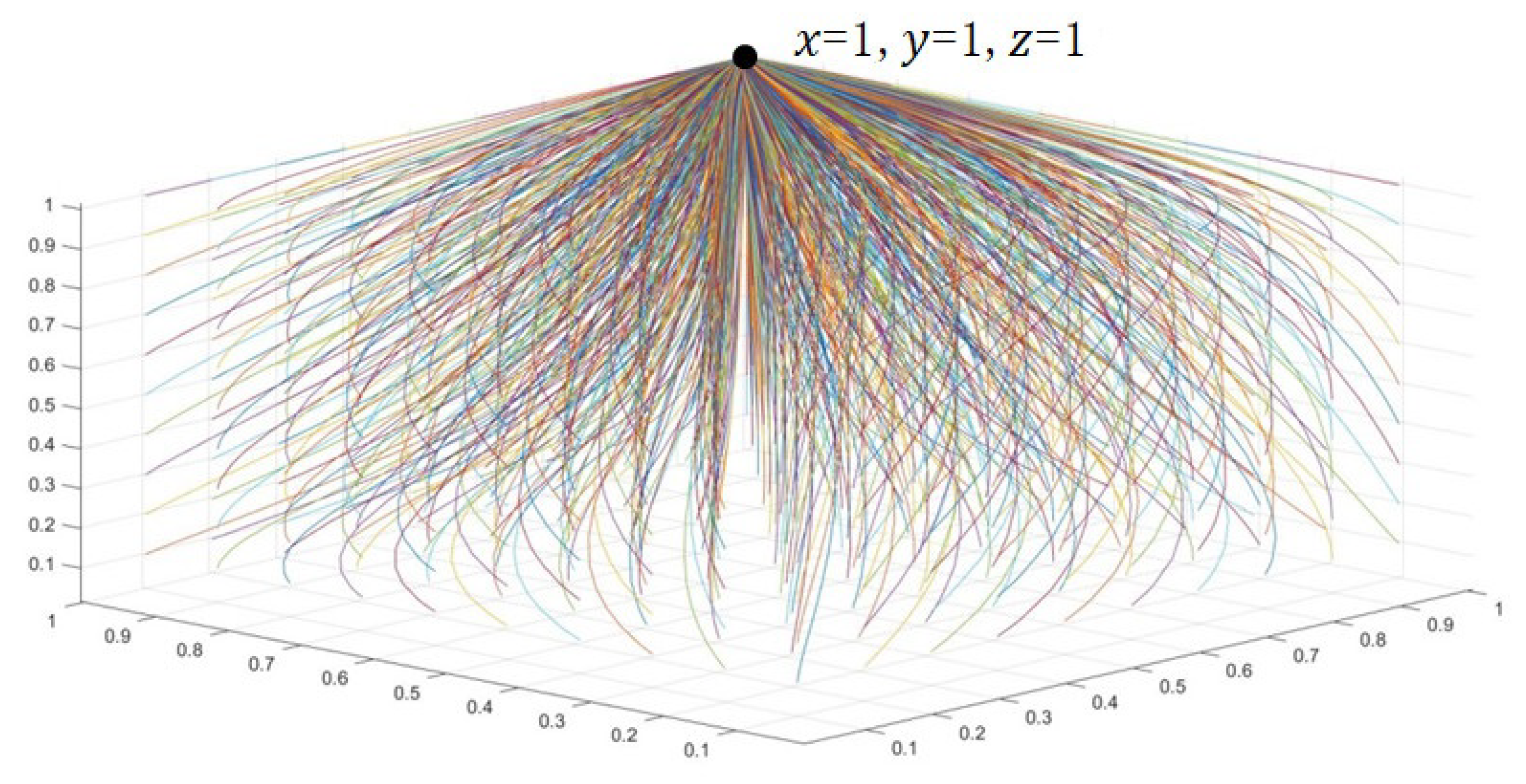
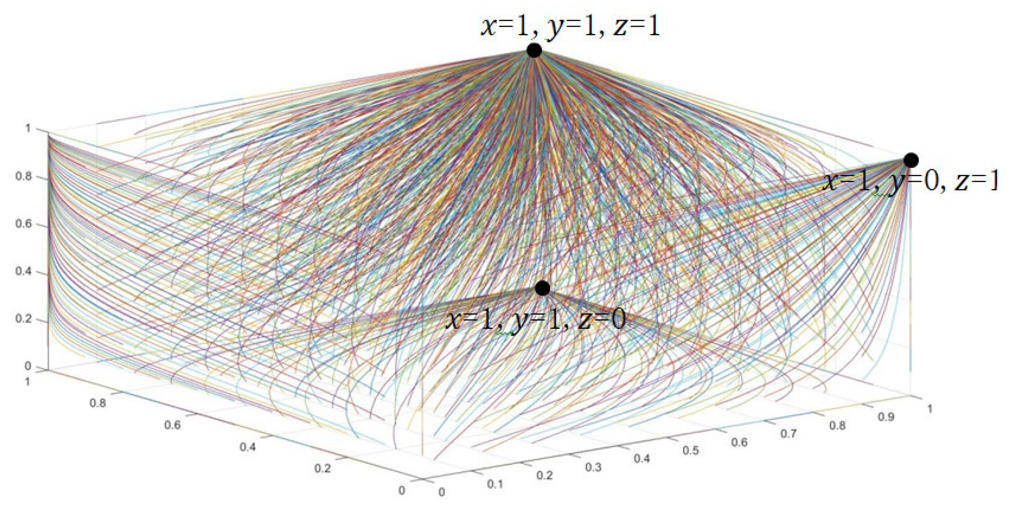
The equilibrium point $E_3$ needs to meet the stability condition: $-i+j<0$, and $\delta >\frac{(u+2\Phi )(1-\overline{\omega })-q}{3}$, let $i=2,j=1,\delta =0.5,\overline{\omega }=0.5,u=2,\Phi =2,q=2$, and make the value of other parameters of the income matrix equal 1, and input the dynamic system (11) into Matlab. The output result is shown in the corresponding points in Figure 1 and Figure 2. It can be seen from the Figure that the final evolution of the system is stable at $E_3(1,1,1)$, meaning that this point is the evolutionary stable strategy (Ess).

5.2. The Stability Simulation of Equilibrium Point $E_6$

(i)

When $\delta <\frac{(u+2\Phi )(1-\overline{\omega })}{3}$, let $u=2,\Phi =1,\overline{\omega }=0.7,\delta =0.3<0.4$, and make the value of other parameters of the income matrix equal 1, and input the dynamic system (12) into Matlab. The output result is shown in the corresponding points in Figure 2. It can be seen from the Figure that the final evolution of the system is stable at $E_6(1,1,0)$, meaning that this point is the evolutionary stable strategy (Ess).

(ii)

When $\overline{\omega }>1-\frac{q+3\delta }{u+2\Phi }$, let $u=2,\Phi =1,q=1.5,\delta =0.5,\overline{\omega }=0.5>0.25$, and make the value of other parameters of the income matrix be 1, and input the dynamic system (13) into Matlab. The output result is shown in the corresponding points in Figure 2. It can be seen from the Figure that the final evolution of the system is stable at $E_6(1,1,0)$, meaning that this point is the evolutionary stable strategy (Ess).

5.3. The Stability Simulation of Equilibrium Point $E_7$

(i)

When $v-2\Phi >0$, $\left\{\begin{array}{c}\hfill \delta <b+(1-\overline{\omega })(d+2h)\\ \hfill \delta <r-(1-\overline{\omega })(v-2\Phi )\end{array}\right.$, let $\overline{\omega }=0.6,b=0.5,d=0.4,h=0.3,r=0.9,v=0.7,\Phi =0.2,\delta =0.5<0.78<0.9$, and make the value of other parameters of the income matrix be 1, and input the dynamic system (14) into Matlab. The output result is shown in the corresponding points in Figure 2. It can be seen from the Figure that the final evolution of the system is stable at $E_7(1,0,1)$, meaning that this point is the evolutionary stable strategy (Ess).

(ii)

When $v-2\Phi <0$, and $\left\{\begin{array}{c}\hfill \frac{b-\delta }{d+2h}+1>\overline{\omega }\\ \hfill \frac{r+\delta }{v-2\Phi }+1>\overline{\omega }\end{array}\right.$, let $v=0.6,\Phi =0.7,b=0.3,d=0.4,h=0.3,r=0.1,\delta =0.5,0.25<\overline{\omega }=0.5<0.8$, and make the value of other parameters of the income matrix be 1, and input the dynamic system (15) into Matlab. The output result is shown in the corresponding points in Figure 2. It can be seen from the Figure that the final evolution of the system is stable at $E_7(1,0,1)$, meaning that this point is the evolutionary stable strategy (Ess).

$$\left\{\begin{array}{c}\hfill 2.5x(1-x)=0\\ \hfill y(1-y)(2-xz)=0\\ \hfill z(1-z)(5.5-0.5x+2xy-y-0.5)=0\end{array}\right.$$

(11)

$$\left\{\begin{array}{c}\hfill x(1-x)(\frac{31}{30}z+2.3)=0\\ \hfill y(1-y)(-2xz+2)=0\\ \hfill z(1-z)(91/30x-xy+0.3)=0\end{array}\right.$$

(12)

$$\left\{\begin{array}{c}\hfill x(1-x)(0.5z+2.5)=0\\ \hfill y(1-y)(-2xz+2)=0\\ \hfill z(1-z)(1.5x+0.5)=0\end{array}\right.$$

(13)

$$\left\{\begin{array}{c}\hfill x(1-x)(0.7y+1.05yz-0.2z+1.8)=0\\ \hfill y(1-y)(-2xz+2)=0\\ \hfill z(1-z)(-x+0.25xy+0.8y+1.3)=0\end{array}\right.$$

(14)

$$r\left\{\begin{array}{c}\hfill x(1-x)(0.7y+1.3yz-0.4z+1.8)=0\\ \hfill y(1-y)(-2xz+2)=0\\ \hfill z(1-z)(-0.4x+1.9xy+0.3y+0.8)=0\end{array}\right.$$

(15)

6. Scenario Analysis of Evolutionary Results

Through the above analysis of the repeated game evolution model and the asymptotic stability of the equilibrium points of the tripartite supply of public goods, the evolutionary stability strategies are obtained, and the evolution path is simulated using Matlab to verify the evolutionary stability. The result shows that the three parties of suppliers, governments, and consumers will tend to adopt the final evolutionary stability strategies under different stability conditions. The three scenarios are:

Scenario 1. The three parties in the game of public goods actively adopt cooperation strategies, that is, suppliers increase low-price supply, the government increases incentives, and consumers actively purchase. When the preconditions are met: $-i+j<0$, and $\delta >\frac{(u+2\Phi )(1-\overline{\omega })-q}{3},E_3(1,1,1)$ is the evolutionary stable strategy (Ess).

According to the values of parameters in the numerical simulation Section 5.1, $\delta >\frac{(u+2\Phi )(1-\overline{\omega })-q}{3}$$=2(1-\overline{\omega })-\frac{2}{3}$ is made known, which means $\delta$ will increase along with the increase of the probability $1-\overline{\omega }$ (the penalty is augmented to punish the betrayer). At this time, the public goods suppliers and the government are more willing to choose a cooperation strategy. The public goods market shows that good features, such as good quality, large output, and low price, can greatly improve the quality of consumers’ lives, which leads to the next round of the repeated game. Therefore, the evolution path of the tripartite supply of public goods eventually evolves and stabilizes at $E_3(1,1,1)$.

Scenario 2. Suppliers and consumers in the game of public goods actively adopt cooperation strategies, while the government adopts betrayal strategies. When the preconditions are met: $\delta <\frac{(u+2\Phi )(1-\overline{\omega })}{3}$ or $\overline{\omega }>1-\frac{q+3\delta }{u+2\Phi }$.

According to the values of parameters in numerical simulation Section 4.2, $\delta <\frac{1-\overline{\omega }}{3}$ or $1-\overline{\omega }<\frac{1.5+3\delta }{4}$ is made known, which means $\delta$ will increase along with the increase of the probability $1-\overline{\omega }$ (the penalty is augmented to punish the betrayer). At this time, the public goods suppliers will actively adopt low-price strategies and increase supply. However, the government will reduce incentives or adopt non-incentive betrayal strategies because supply exceeds demand. In this case, prices fall, and then consumer purchase costs decrease, which eventually result in an increase in profits. This situation then leads to the next round of repeated games. Therefore, the evolution path of the tripartite supply of public goods eventually evolves and stabilizes at $E_6(1,1,0)$.

Scenario 3. Suppliers and the government in the game of public goods actively adopt cooperation strategies, while consumers adopt evolutionary strategies from purchasing to non-purchasing strategies.

According to the values of parameters in numerical simulation Section 4.3, $\delta <0.9-0.3(1-\overline{\omega })$ or $(1-\overline{\omega })>0.125-1.25\delta$ is made known, which means $\delta$ will increase along with the increase of the probability $1-\overline{\omega }$ (the penalty is augmented to punish the betrayer). At this time, the public goods suppliers will actively increase supply in low price and the government is willing to provide incentives. However, consumers adopt non-purchase betrayal strategies. In this case, the public goods market presents good features, such as good quality, large output, favorable price, and government incentives. These types of goods are oversaturated and consumers are reluctant to buy them. This leads to the next round of repeated games. Therefore, the evolution path of the tripartite supply of public goods eventually evolves and stabilizes at $E_7(1,0,1)$.

7. Conclusions

On the basis of replicate dynamics of evolutionary games and repeated games, as well as pertinent content, a tripartite repeated game model is established based on the existing tripartite game among suppliers, consumers, and the government to analyze the evolutionary mechanism of which suppliers supply at low prices, consumers purchase, and the government provides incentives. A dynamic system of repeated games was thereby established to analyze the stability of the equilibrium point of the tripartite repeated evolutionary game under different parameters. A numerical simulation and scenario analysis were employed to verify the impact of penalty coefficients and discount factors on the stability of strategies adopted by the three players in a tripartite repeated game on public goods. The research results of this paper are of great significance for the infinitely repeated behavior of population game players in the supply chain of public goods, such as coal, water, electricity, and gas. This paper is also helpful to provide a reference for decision-makers in the game on public goods in the market economy.

Due to the large amount of calculation, the game only considers the impact of penalty coefficients and discount factors on the government and suppliers, but not their impact on consumers. At the same time, the game does not consider the situation where the government or the supplier needs to pay the penalty cost when the penalty is imposed.

As an extension of this study, in the next step, we will consider the case that the player needs to pay the penalty cost in the study of the principal-agent repeated game theory of public goods. In addition, the tripartite game behavior of the government, power generation companies (hydropower or thermal power), and the power supply department in the quasi-public goods-electricity supply market will be taken as an example for application analysis and research.

References

- Schein, B.M.; Teclezghi, B. Endomorphisms of finite symmetric inverse semigroups. J. Algebra 1997, 198, 300–310. [Google Scholar] [CrossRef] [Green Version]
- Schein, B.M.; teclezghi, B.M.; Teclezghi, B. Endomorphisms of finite full transformation semigroups. Proc. Am. Math. Soc. 1998, 126, 2579–2587. [Google Scholar] [CrossRef]
- Taylor, P.D.; Jonker, L.B. Evolutionary stable strategies and game dynamics. Math. Biosci. 1978, 40, 145–156. [Google Scholar] [CrossRef]
- Gordon and Breach. Transportation Planning and Technology. Book Rev. 1979, 5, 183–187. [Google Scholar]
- Friedman, J.W. A Non-cooperative Equilibrium for Super games. Rev. Econ. Stud. 1971, 38, 1–12. [Google Scholar] [CrossRef]
- Abreu, D. On the Theory of In finitely Repeated Game swith Discounting. Econometrica 1983, 56, 383–396. [Google Scholar] [CrossRef]
- Fudenberg, D.; Maskin, E. The folk the oremin repeated game swith discounting or with in complete information. J. Econom. Soc. 1986, 54, 533–554. [Google Scholar] [CrossRef] [Green Version]
- Zhang, Z.; Yang, H. Hopf bifurcation of a predator-prey system with delays and stage structure for the prey. Discret. Dyn. Nat. Soc. 2012, 55, 327–337. [Google Scholar] [CrossRef]
- Junhai, M.; Ying, W.; Wei, X. Research on the triopoly dynamic Game model based on different rationalities and its chaos control. Wseas Trans. Math. 2014, 13, 983–991. [Google Scholar]
- Zhu, Y. R& D Competition and Cooperation among Members in Supply Chain Based on Evolutionary Game. J. Guangdong Univ. Technol. 2015, 3, 46–50. [Google Scholar]
- Wu, J. Research on the Collaborative Innovation Mechanism of Government, Industry, University and Research Institute Based on Three-Group Evolutionary Game. Chin. J. Manag. Sci. 2019, 1, 162–173. [Google Scholar]
- Xiao, J. Evolutionary Game Theory between Local Governments under Single Direction Spillover of Public Goods: A Case Study of the Water Resource Ecological Compensation across Regions. Theory Pract. Financ. Econ. 2016, 6, 96–101. [Google Scholar]
- Shi, Y.; Zhu, J. Game-theoretic analysis for supply chain with distributionalal and peer-induced fairness concerned retailers. Manag. Sci. Eng. 2014, 8, 78–84. [Google Scholar]
- Pu, X.; Gong, L.; Han, G. A feasible incentive contract between a manufacturer and his fairness-sensitive retailer engaged in strategic marketing efforts. J. Intell. Manuf. 2019, 30, 193–206. [Google Scholar] [CrossRef]
- Yu, J.; Yuan, X.Z.; Isac, G. The stability of solutions for differential inclusions and differential equations in the sense of Baire category theory. Appl. Math. Lett. 1998, 11, 51–56. [Google Scholar] [CrossRef] [Green Version]
- Yu, J.; Xiang, S.W. On essential components of the set of Nash equilibrium points. Nonlinear Anal. Theory Methods Appl. 1999, 38, 259–264. [Google Scholar] [CrossRef]
- Yang, H.; Yu, J. On essential components of the set of weakly Pareto-Nash equilibrium points. Appl. Math. Lett. 2002, 15, 303–310. [Google Scholar] [CrossRef] [Green Version]
- Yu, J.; Yang, H.; Yu, C. Structural stability and robustness to bounded rationality for non-compact cases. J. Glob. Optim. 2009, 44, 149–157. [Google Scholar] [CrossRef]
- Yang, H.; Yu, J. Unified approaches to well-posedness with some applications. J. Glob. Optim. 2005, 31, 371–381. [Google Scholar] [CrossRef]
- Song, Q.Q.; Guo, M.; Chen, H.Z. Essential sets of fixed points for correspondences with applications to Nash equilibria. Fixed Point Theory 2016, 17, 141–150. [Google Scholar]
- Yang, Z.; Wang, A.Q. Existence and stability of the Ccore for fuzzy games. Fuzzy Sets Syst. 2018, 341, 59–68. [Google Scholar] [CrossRef]
- Zhong, C.; Yang, H.; Wang, C. Refinements of Equilibria for Population Games Based on Bounded Rationality. Math. Probl. Eng. 2020, 1636294. [Google Scholar] [CrossRef]
- Jin, X.; Yu, J. Dissymmetrical Information, Effectiveness of Reputation and Balanced Cooperation. Soc. Sci. Front. Econ. Stud. 2004, 1, 70–75. [Google Scholar]
- Laclaua, M.; Tomala, T. Repeated games with public determonistic monitoring. J. Econ. Theory 2017, 169, 400–424. [Google Scholar] [CrossRef]
- Khakzad, H. Repeated games foreco-friendly flushing in reservoirs. Water Pract. Technol. 2019. [Google Scholar] [CrossRef]
- Juan, F.; Escobara, L.; lanes, G. Cooperation dynamics in repeated games of adver seselection. J. Econ. Theory 2018, 176, 408–443. [Google Scholar]
Figure 1.
Path of numerical simulation.
Figure 2.