Delay in a 2-State Discrete-Time Queue with Stochastic State-Period Lengths and State-Dependent Server Availability and Arrivals

Abstract

In this paper, we consider a discrete-time multiserver queueing system with correlation in the arrival process and in the server availability. Specifically, we are interested in the delay characteristics. The system is assumed to be in one of two different system states, and each state is characterized by its own distributions for the number of arrivals and the number of available servers in a slot. Within a state, these numbers are independent and identically distributed random variables. State changes can only occur at slot boundaries and mark the beginnings and ends of state periods. Each state has its own distribution for its period lengths, expressed in the number of slots. The stochastic process that describes the state changes introduces correlation to the system, e.g., long periods with low arrival intensity can be alternated by short periods with high arrival intensity. Using probability generating functions and the theory of the dominant singularity, we find the tail probabilities of the delay.

1. Introduction

When, in the early 20th century, the Danish mathematician Agner Erlang used a mathematical model to describe a telephone switch (at the time, an office where workers manually connected phone lines), he became the founder of the field of queueing theory. More than a hundred years later, queueing theory is used in a broad range of practical problems such as in traffic engineering and industrial engineering, but telecommunications remains one of the main fields of application [1,2,3].

Multiserver queueing models have received considerable attention in the past. Most papers, however, focus on the analysis of the queue length characteristics only. Results are available for queueing systems with a constant number of available servers [4,5,6] as well as for queueing systems with a variable number of available servers [7,8,9].

When it comes to delay analysis, multiserver queueing systems are notoriously hard to analyze, but some results do exist in the literature. In [10,11,12], discrete-time queueing systems are treated where the number of available servers is constant, while in [13], the number of available servers in a slot is a stochastic variable which is independent and identically distributed (i.i.d.) from slot to slot. In [14], a continuous-time queueing system is treated where N servers are subject to breakdowns and repair; the results are the distributions of the queue length and waiting times. The authors of [15] obtain the queue length distribution and the delay distribution for a discrete-time model with general service demands and correlated service capacities. In their model, the service time of a customer depends on both its service demand and the service capacity.

In this paper, we consider a discrete-time multiserver queueing system that is special in the way that it allows correlation in both the slot-to-slot server availability and the arrival process. The buffer capacity is assumed to be infinite and the queueing discipline is First Come First Served (FCFS). In our earlier paper [16], we handled the system content of such a queueing system, and now we focus on the analysis of the delay characteristics.

Table 1. Brief summary of the setting and delay results of relevant papers in comparison with the current paper.

Paper	Servers	Arrivals	Delay Results
Chaudhry et al. [10]	constant	general (bulk), i.i.d.	full delay distribution
Bruneel et al. [11]	constant	general, i.i.d.	tail probabilities
Gao et al. [12]	constant	general, i.i.d.	tail probabilities
Laevens et al. [13]	i.i.d.	general, i.i.d.	tail probabilities
Neuts et al. [14]	i.i.d.	general, i.i.d.	full delay distribution
De Muynck et al. [15]	correlated	general, i.i.d.	full delay distribution
The current paper	correlated	correlated	tail probabilites

compares the setting and delay results of the current paper to those of the relevant related papers indicated above.

The considered queueing system can be in two different system states. For every slot, a stochastic number of servers is available, and a stochastic number of new customers arrive. These are both i.i.d. within each state, but these distributions can be different for each state. The system resides for a stochastic number of slots in the same state before state transitions occur, which can only happen at slot boundaries. The sojourn times follow a distribution which is also dependent on the system state.

The above setup can be used to model a wide variety of queueing systems, such as queues with bursty arrivals (where long periods of low/no arrival intensity are alternated by short periods of high arrival intensity) and queues with cyclical service capacities (where alternately few and many servers are available for fixed period lengths).

The potential applications can be found in many fields. In [17,18], continuous time models are used to calculate the delay in a system with time-varying arrival intensity and service capacity. The envisaged application is a hospital emergency department, but the model can also be used in other applications. In [19], time-dependent arrival rates are called a key feature of many real life service systems and it is, therefore, included in the Erlang loss model which is presented. In [20], an overview of time-varying queueing models is presented, from a telecommunications point of view. A possible application of the method of this paper is a processor sharing system with speed scaling [21], where the processing speed is adapted to the (expected) load. Another possible application is the domain of mobile ad hoc networks [22]. In such networks, nodes (which can move freely) must cooperate to send and receive packages. The number of available nodes as well as the traffic varies over time.

The outline of the paper is as follows. In Section 2, we give the mathematical outline of the queueing model. In Section 3, we repeat some key results regarding the system content from our earlier paper [16]. In Section 4, we condition the delay of a customer on the state of the arrival slot and on the number of customers present in the queue at the moment of arrival. Section 5 then describes how the delay of an arbitrary customer can be obtained. In Section 6, we use the theory of the dominant singularity to obtain the tail characteristics of the delay. The numerical examples in Section 7 illustrate the model and Section 8 concludes the paper.

2. Queueing Model

We consider the discrete-time multiserver queueing model of [16] with correlation over time in both the arrival process and the server availability. In this discrete-time model, the time horizon is divided into slots of equal length and, during a slot, the system can be either in state 1 or state 2. Note that, in general, in our paper, we will always use i to indicate a system state and not repeat that it can only take values 1 and 2. Furthermore, we will use $\overline{ı}$ to refer to the other state:

$$\begin{array}{c}\hfill \overline{ı} \triangleq 3-i.\end{array}$$

(1)

Therefore, put simply, there are two types of slots, which we call state-1-slots and state-2-slots, and during a state-i-slot the queueing system is in system state i. State changes can only occur at slot boundaries and mark the beginnings and ends of state-1-periods and state-2-periods. If we denote with $r_{i,k}$ the length (expressed in the number of slots) of the kth state-i-period, then the series $\left\{r_{i,k}\right\}$ form two sets of i.i.d. stochastic variables. Their distribution is given by

$$r_i\left(n\right) \triangleq \mathrm{Prob} \left[\mathrm{state}-i-\mathrm{period} \mathrm{has} n \mathrm{slots}\right],\hspace{1em}n\ge 1;$$

(2)

$$R_i \left(z\right) \triangleq \sum _{n=1}^{\infty }{r}_i\left(n\right)z^n;\hspace{1em}{\overline{r}}_i \triangleq \sum _{n=1}^{\infty }n{r}_i\left(n\right) =R_i^{\prime } \left(1\right),$$

(3)

where we have introduced the probability generating functions (pgfs) $R_i\left(z\right)$. We limit the $R_i\left(z\right)$ to be rational functions of their argument:

$$\begin{array}{c}\hfill R_i \left(z\right) =\frac{A_r^i \left(z\right)}{B_r^i \left(z\right)},\end{array}$$

(4)

with $A_r^i\left(z\right)$ and $B_r^i\left(z\right)$ mutually prime polynomials of degree $m_{Ar}^i$ and $m_{Br}^i$, respectively, and with $A_r^i\left(1\right) =B_r^i\left(1\right) =1$. We define $m_r^i$ as:

$$\begin{array}{c}\hfill m_r^i \triangleq \max (m_{Ar}^i,m_{Br}^i).\end{array}$$

(5)

The probability that an arbitrary slot belongs to a given state is equal to the fraction of time the system is in that state and is given by

$$\begin{array}{c}\hfill {\sigma }_i \triangleq \mathrm{Prob} \left[\mathrm{arbitrary} \mathrm{slot} \mathrm{belongs} \mathrm{to} \mathrm{state} i\right] =\frac{{\overline{r}}_i}{{\overline{r}}_1+{\overline{r}}_2}.\end{array}$$

(6)

The special feature of our model is that the server availability and the arrival process both depend on the system state. Specifically, the distribution of the number of available servers during a slot depends on the system state during that slot in the following way:

$$s_i\left(n\right) \triangleq \mathrm{Prob} \left[n \mathrm{servers} \mathrm{available} \mathrm{during} \mathrm{a} \mathrm{state}-i-\mathrm{slot}\right],\hspace{1em}n\ge 1;$$

(7)

$$S_i \left(z\right) \triangleq \sum _{n=1}^{\infty }{s}_i\left(n\right)z^n;\hspace{1em}{\overline{s}}_i \triangleq \sum _{n=1}^{\infty }n{s}_i\left(n\right) =S_i^{\prime } \left(1\right).$$

(8)

During every slot, there is at least one server available and within a given state-i-period the numbers of available servers during the different slots are i.i.d. from slot to slot. Similarly to the $R_i\left(z\right)$, we also limit the $S_i\left(z\right)$ to be rational functions of their argument:

$$\begin{array}{c}\hfill S_i \left(z\right) =\frac{A_s^i \left(z\right)}{B_s^i \left(z\right)},\end{array}$$

(9)

with $A_s^i\left(z\right)$ and $B_s^i\left(z\right)$ mutually prime polynomials of degree $m_{As}^i$ and $m_{Bs}^i$, respectively, and with $A_s^i\left(1\right) =B_s^i\left(1\right) =1$. We define $m_s^i$ as:

$$\begin{array}{c}\hfill m_s^i \triangleq \max (m_{As}^i,m_{Bs}^i).\end{array}$$

(10)

The numbers of arrivals during the different slots of a given state-i-period are i.i.d. from slot to slot as well. Their common distribution is characterized by

$$c_i\left(n\right) \triangleq \mathrm{Prob} \left[\mathrm{state}-i-\mathrm{slot} \mathrm{has} n \mathrm{arrivals}\right],\hspace{1em}n\ge 0;$$

(11)

$$C_i \left(z\right) \triangleq \sum _{n=0}^{\infty }{c}_i\left(n\right)z^n;\hspace{1em}{\lambda }_i \triangleq \sum _{n=1}^{\infty }n{c}_i\left(n\right) =C_i^{\prime } \left(1\right).$$

(12)

The average arrival intensity is then given by

$$\begin{array}{c}\hfill \lambda \triangleq {\sigma }_1{\lambda }_1+{\sigma }_2{\lambda }_2.\end{array}$$

(13)

Customers can only start service at slot boundaries, so an arriving customer can only be taken into service at the beginning of the next slot, even if a server is idle at the moment of arrival. The queue capacity is assumed to be infinite, so an arriving customer will always join the system. Each customer requires exactly one slot of service.

We assume the system reaches steady state and, therefore, the average number of customers entering the system should be strictly smaller than the average number of available servers [23], leading to the following stability condition:

$$\begin{array}{c}\hfill \lambda <{\sigma }_1{\overline{s}}_1+{\sigma }_2{\overline{s}}_2.\end{array}$$

(14)

Furthermore, it will prove useful to introduce the following notation:

$$\begin{array}{c}\hfill Y_i \left(z\right) \triangleq C_i \left(z\right)S_i \left(\frac{1}{z}\right).\end{array}$$

(15)

3. System Content

In an earlier work [16], we analyzed the system content for a queueing model as described above. In the current section, we repeat the main results that are necessary for the delay analysis in this paper. Let us denote with the stochastic variable $g_k^i$ ($k\ge 0$), the total number of customers in the system at the beginning of the $(k+1)$st slot of a state-i-period. The corresponding pgf is $G_k^i\left(z\right)$. We can derive the following recursive equation, valid for $k\ge 1$:

$$\begin{array}{c}\hfill G_k^i \left(z\right) =Y_i \left(z\right)G_{k-1}^i \left(z\right)+C_i \left(z\right)\sum _{l=0}^{\infty }\sum _{j=1}^{\infty }\mathrm{Prob}[g_{k-1}^i = l]s_i(l+j)\left(1-z^{-j}\right).\end{array}$$

(16)

We can obtain a set of two linear equations for the functions $G_0^i\left(z\right)$ by recursive application of (16) and by stating that the system content at the beginning of a state-i-period equals the system content at the end of a state-$\overline{ı}$-period. This set of equations can then be solved to yield the following expression:

$$\begin{array}{c}\hfill G_0^i \left(z\right) =\frac{S_{\overline{ı}} \left(\frac{1}{z}\right)R_{\overline{ı}} \left(Y_{\overline{ı}} \left(z\right)\right)\left[Q_i \left(Y_i \left(z\right),1\right)-Q_i \left(Y_i \left(z\right),\frac{1}{z}\right)\right]+S_i \left(\frac{1}{z}\right)\left[Q_{\overline{ı}} \left(Y_{\overline{ı}} \left(z\right),1\right)-Q_{\overline{ı}} \left(Y_{\overline{ı}} \left(z\right),\frac{1}{z}\right)\right]}{S_i \left(\frac{1}{z}\right)S_{\overline{ı}} \left(\frac{1}{z}\right)\left[1-R_i \left(Y_i \left(z\right)\right)R_{\overline{ı}} \left(Y_{\overline{ı}} \left(z\right)\right)\right]},\end{array}$$

(17)

with the bivariate functions $Q_i \left(x,z\right)$ unknown. It can be proven that if $R_i\left(z\right)$ and $S_i\left(z\right)$ are rational functions of their argument, then also the $Q_i \left(x,z\right)$ are rational and of the following form:

$$\begin{array}{c}\hfill Q_i \left(x,z\right) =\frac{A_q^i \left(x,z\right)}{B_r^i \left(x\right)B_s^i \left(z\right)};\hspace{1em}{A}_q^i \left(x,z\right) \triangleq \sum _{n=1}^{m_r^i}\sum _{j=1}^{m_s^i}{ϵ}_{nj}^i{x}^n{z}^j.\end{array}$$

(18)

The (finite number of) unknowns ${ϵ}_{nj}^i$ can be determined by relying on the properties of pgfs, namely that they are normalized and that they are analytical within the complex unit disk. To do this, the roots within the complex unit disk of the denominator of (17) need to be determined and a set of linear equations needs to be solved. For many common choices of the distributions in the model, this does not require large computational effort. Similarly, it is possible to obtain the pgfs of the system content at the beginning of an arbitrary state-i-slot and at the beginning of an arbitrary slot. Based on these pgfs, important performance metrics can be calculated, such as the expected number of customers in the system.

4. Delay of a Customer with $\mathit{K}$ Customers Ahead

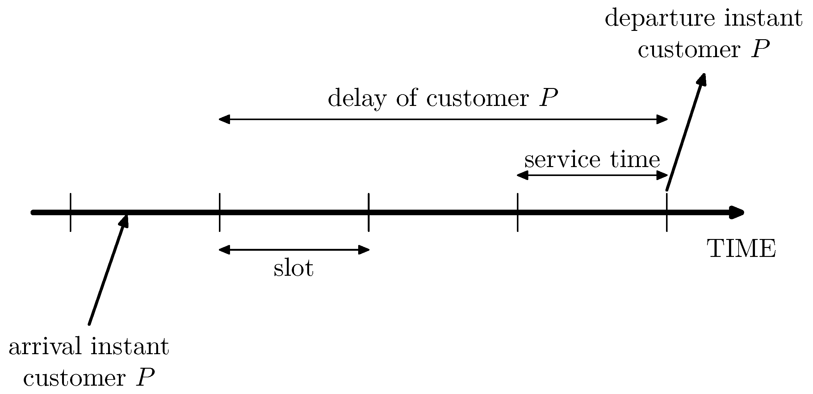
For the system content, the specific queueing discipline is not of importance, as long as it is work conserving. However, for the delay analysis it needs to be specified. We will assume a First Come First Served (FCFS) policy. We do not specify the exact arrival instant of a customer within a slot and, therefore, define its delay as the time interval from the first slot boundary after the customer’s arrival until the end of its service slot. This definition is illustrated in Figure 1. The delay thus consists of an integer number of slots and is at least one slot long. This setup is also referred to as a Late Arrival System with Delayed Access (LAS-DA) [24].

Let us denote with the stochastic variable $d_k^{i,n}$ the delay of a customer that arrives during a state-i-slot, with n more slots until the next state-$\overline{ı}$-slot and with k customers waiting in the queue with priority over the arriving customer (excluding the customer(s) currently in service, if any). The corresponding pgf is $D_k^{i,n}\left(z\right)$. Clearly, if during the slot after the considered customer’s arrival slot more than k servers are available, the customer’s delay will consist of exactly one slot. Otherwise, if during the first delay slot only $l\le k$ servers are available, there will be an additional number of delay slots that corresponds to the delay of a customer with $k-l$ customers ahead. Based on these observations, we can state

$$\begin{array}{cc}\hfill D_0^{i,n} \left(z\right) =& z;\hfill \end{array}$$

(19)

$$\begin{array}{cc}\hfill D_k^{i,n} \left(z\right) =& z\sum _{l=k+1}^{\infty }{s}_i\left(l\right)+z\sum _{l=1}^k{D}_{k-l}^{i,n-1} \left(z\right)s_i\left(l\right),\hspace{1em}k,n\ge 1;\hfill \end{array}$$

(20)

$$\begin{array}{cc}\hfill D_k^{i,0} \left(z\right) =& z\sum _{l=k+1}^{\infty }{s}_{\overline{ı}}\left(l\right)+z\sum _{n=1}^{\infty }{r}_{\overline{ı}}\left(n\right)\sum _{l=1}^k{D}_{k-l}^{\overline{ı},n-1} \left(z\right)s_{\overline{ı}}\left(l\right),\hspace{1em}k\ge 1.\hfill \end{array}$$

(21)

Furthermore, we use the stochastic variable $d_k^i$ for the delay of a customer arriving during the first slot of a state-i-period and with k customers in the queue with priority over the arriving customer. The corresponding pgf $D_k^i\left(z\right)$ can be expressed as

$$\begin{array}{c}\hfill D_k^i \left(z\right) = \sum _{n=1}^{\infty }{r}_i\left(n\right)D_k^{i,n-1} \left(z\right).\end{array}$$

(22)

Let us now introduce two auxiliary functions

$$\begin{array}{cc}\hfill D^{i,n} \left(x,z\right)& \triangleq \sum _{k=0}^{\infty }{D}_k^{i,n} \left(z\right)x^k;\hfill \end{array}$$

(23)

$$\begin{array}{cc}\hfill D^i \left(x,z\right)& \triangleq \sum _{k=0}^{\infty }{D}_k^i \left(z\right)x^k\hfill \\ & =\sum _{n=1}^{\infty }\sum _{k=0}^{\infty }{r}_i\left(n\right)D_k^{i,n-1} \left(z\right)x^k=\sum _{n=1}^{\infty }{r}_i\left(n\right)D^{i,n-1} \left(x,z\right).\hfill \end{array}$$

(24)

Using the Relations (19) and (20), we obtain

$$\begin{array}{c}\hfill D^{i,n} \left(x,z\right) =z{S}_i \left(x\right)D^{i,n-1} \left(x,z\right)+z\frac{1-S_i \left(x\right)}{1-x},\hspace{1em}n\ge 1.\end{array}$$

(25)

After recursive application this leads to

$$\begin{array}{c}\hfill D^{i,n} \left(x,z\right) ={\left[z{S}_i \left(x\right)\right]}^n{D}^{i,0} \left(x,z\right)+z\frac{1-{\left[z{S}_i \left(x\right)\right]}^n}{1-z{S}_i \left(x\right)} \frac{1-S_i \left(x\right)}{1-x},\hspace{1em}n\ge 0.\end{array}$$

(26)

Multiplying (26) with $r_i(n+1)$ and summing over all $n\ge 0$ we get

$$\begin{array}{c}\hfill D^i \left(x,z\right) =\frac{1}{z{S}_i \left(x\right)}{R}_i \left(z{S}_i \left(x\right)\right)D^{i,0} \left(x,z\right)+z\frac{1-S_i \left(x\right)}{(1-x)\left[1-z{S}_i \left(x\right)\right]}\left[1-\frac{R_i \left(z{S}_i \left(x\right)\right)}{z{S}_i \left(x\right)}\right].\end{array}$$

(27)

Using (21) we can also work out an expression for $D^{i,0} \left(x,z\right)$:

$$\begin{array}{c}\hfill D^{i,0} \left(x,z\right) =z{S}_{\overline{ı}} \left(x\right)D^{\overline{ı}} \left(x,z\right)+z\frac{1-S_{\overline{ı}} \left(x\right)}{1-x}.\end{array}$$

(28)

Combining (27) and (28) we then obtain the following set of equations:

$$\begin{array}{c}\hfill D^i \left(x,z\right) =\frac{1}{S_i \left(x\right)}{R}_i \left(z{S}_i \left(x\right)\right)\left[S_{\overline{ı}} \left(x\right)D^{\overline{ı}} \left(x,z\right)+\frac{1-S_{\overline{ı}} \left(x\right)}{1-x}\right]+z\frac{1-S_i \left(x\right)}{(1-x)\left[1-z{S}_i \left(x\right)\right]}\left[1-\frac{R_i \left(z{S}_i \left(x\right)\right)}{z{S}_i \left(x\right)}\right],\end{array}$$

(29)

which can be solved to find an explicit expression for $D^i \left(x,z\right)$:

$$\begin{array}{c}\hfill D^i \left(x,z\right) =\frac{{\tilde{f}}^i \left(x,z\right)}{{\tilde{g}}^i \left(x,z\right)},\end{array}$$

(30)

with

$$\begin{array}{cc}\hfill {\tilde{f}}^i \left(x,z\right) =& z^2{S}_i \left(x\right)S_{\overline{ı}} \left(x\right)R_i \left(z{S}_i \left(x\right)\right)R_{\overline{ı}} \left(z{S}_{\overline{ı}} \left(x\right)\right)\left[1-S_i \left(x\right)\right]+z{S}_i {\left(x\right)}^2{R}_i \left(z{S}_i \left(x\right)\right)R_{\overline{ı}} \left(z{S}_{\overline{ı}} \left(x\right)\right)\hfill \\ & \hspace{1em}+z^2{S}_i {\left(x\right)}^2{S}_{\overline{ı}} \left(x\right)-z{S}_{\overline{ı}} \left(x\right)R_i \left(z{S}_i \left(x\right)\right)R_{\overline{ı}} \left(z{S}_{\overline{ı}} \left(x\right)\right)-z^2{S}_i \left(x\right)S_{\overline{ı}} \left(x\right)\hfill \\ & \hspace{1em}+R_i \left(z{S}_i \left(x\right)\right)\left[R_{\overline{ı}} \left(z{S}_{\overline{ı}} \left(x\right)\right)+z-1\right]\left[S_{\overline{ı}} \left(x\right)-S_i \left(x\right)\right]-z{S}_i {\left(x\right)}^2+z{S}_i \left(x\right);\hfill \end{array}$$

(31)

$$\begin{array}{cc}\hfill {\tilde{g}}^i \left(x,z\right) =& S_i \left(x\right)(1-x)\left[1-z{S}_i \left(x\right)\right]\left[1-z{S}_{\overline{ı}} \left(x\right)\right]\left[1-R_i \left(z{S}_i \left(x\right)\right)R_{\overline{ı}} \left(z{S}_{\overline{ı}} \left(x\right)\right)\right].\hfill \end{array}$$

(32)

Note that ${\tilde{f}}^i \left(x,z\right)$ is divisible by $S_i\left(x\right)$ as $R_i\left(0\right) =0$. Bearing in mind that all pgfs are normalized, we can furthermore verify that ${\tilde{f}}^i \left(x,z\right)$ is divisible by $(1-x)$, $(1-z{S}_i\left(x\right))$ and $(1-z{S}_{\overline{ı}}\left(x\right))$. In order to rewrite (30) as a rational function of x, we divide numerator and denominator by those common factors. To remove the remaining poles in x in ${\tilde{g}}^i \left(x,z\right)$, we multiply with the auxiliary function $u \left(x,z\right)$, which in view of (4) and (9) is defined as

$$\begin{array}{c}\hfill u(x,z) \triangleq B_r^i \left(z{S}_i \left(x\right)\right)B_r^{\overline{ı}} \left(z{S}_{\overline{ı}} \left(x\right)\right)B_s^i {\left(x\right)}^{m_r^i}{B}_s^{\overline{ı}} {\left(x\right)}^{m_r^{\overline{ı}}}.\end{array}$$

(33)

Therefore, we obtain

$$\begin{array}{c}\hfill D^i \left(x,z\right) =\frac{f^i \left(x,z\right)}{g \left(x,z\right)},\end{array}$$

(34)

with

$$\begin{array}{cc}\hfill f^i \left(x,z\right) =& \frac{{\tilde{f}}^i \left(x,z\right)u \left(x,z\right)}{S_i \left(x\right)(1-x)\left[1-z{S}_i \left(x\right)\right]\left[1-z{S}_{\overline{ı}} \left(x\right)\right]};\hfill \end{array}$$

(35)

$$\begin{array}{cc}\hfill g \left(x,z\right) =& \left[1-R_i \left(z{S}_i \left(x\right)\right)R_{\overline{ı}} \left(z{S}_{\overline{ı}} \left(x\right)\right)\right]u \left(x,z\right).\hfill \end{array}$$

(36)

The new denominator $g \left(x,z\right)$ of $D^i \left(x,z\right)$ is a polynomial in x of degree $M \triangleq m_s^i{m}_r^i+m_s^{\overline{ı}}{m}_r^{\overline{ı}}$ and the numerator is of degree $M-1$. We can do a partial fraction expansion of $D^i \left(x,z\right)$ based on its poles $x_{\varphi }$ in x, which we assume distinct. Note that the $x_{\varphi }$ ($\varphi =1,\dots ,M$) are functions of z, but for notational simplicity the argument is omitted. We can then write $D^i \left(x,z\right)$ as

$$\begin{array}{c}\hfill D^i \left(x,z\right) =\sum _{\varphi =1}^M\frac{f^i \left(x_{\varphi },z\right)}{g_x \left(x_{\varphi },z\right)(x-x_{\varphi })},\end{array}$$

(37)

with

$$\begin{array}{c}\hfill g_x \left(x,z\right) \triangleq \frac{\partial }{\partial x}g \left(x,z\right).\end{array}$$

(38)

The above allows us to easily obtain an expression for $D_k^i\left(z\right)$, which is the pgf of the delay of a customer arriving during the first slot of a state-i-period with k customers waiting in the queue with priority over the considered customer:

$$\begin{array}{c}\hfill D_k^i \left(z\right) =\frac{1}{k!}{\left.\frac{{\partial }^k}{\partial x^k}{D}^i \left(x,z\right)\right|}_{x=0}=\sum _{\varphi =1}^M\frac{-f^i \left(x_{\varphi },z\right)}{x_{\varphi }^{k+1}{g}_x \left(x_{\varphi },z\right)}.\end{array}$$

(39)

5. Delay of an Arbitrary Customer

Let us now consider the arbitrary customer P, arriving during slot S. We denote the probability that S is a state-i-slot with $h^i$ and that it is the lth slot of a state-i-period of in total $l+n$ slots as $h_{l|n}^i$:

$$\begin{array}{cc}\hfill h^i \triangleq & \mathrm{Prob} \left[P \mathrm{arrives} \mathrm{during} \mathrm{state}-i-\mathrm{slot}\right] =\frac{{\lambda }_i{\overline{r}}_i}{{\lambda }_1{\overline{r}}_1+{\lambda }_2{\overline{r}}_2};\hfill \end{array}$$

(40)

$$\begin{array}{cc}\hfill h_{l|n}^i& \triangleq \mathrm{Prob} \left[P \mathrm{arrives} \mathrm{during} l\mathrm{th} \mathrm{slot} \mathrm{of} \mathrm{state}-i-\mathrm{period} \mathrm{with} n+l \mathrm{slots} \mathrm{in} \mathrm{total}\right]\hfill \\ & =h^i\frac{r_i(n+l)}{{\overline{r}}_i}.\hfill \end{array}$$

(41)

The pgf $F_i\left(z\right)$ of the number of customers that arrive during slot S but before customer P and given that S is a state-i-slot is known to be given by (see, e.g., [1])

$$\begin{array}{c}\hfill F_i \left(z\right) =\frac{C_i \left(z\right)-1}{{\lambda }_i(z-1)}.\end{array}$$

(42)

The queue content as experienced by P upon arrival, are the customers with priority over P that can start service after S. It thus consists of the customers that were present in the system at the beginning of S, minus those that receive service during S and plus those that arrived during S but before P. It is a stochastic variable that depends on the state of S and on the time since the last state change. Given that S is the lth slot of a state-i-period, we will denote this stochastic variable as $t_l^i$ ($l\ge 1$). Its pgf $T_l^i\left(z\right)$ can be obtained by translating the above observations into the z-domain:

$$\begin{array}{cc}\hfill T_l^i \left(z\right)& =F_i \left(z\right)\sum _{k=0}^{\infty }\mathrm{Prob} \left[g_{l-1}^i=k\right]\left\{\sum _{j=1}^k{s}_i\left(j\right)z^{k-j}+\sum _{j=1}^{\infty }{s}_i(k+j)\right\}\hfill \\ & =F_i \left(z\right)G_{l-1}^i \left(z\right)S_i \left(\frac{1}{z}\right)+F_i \left(z\right)\sum _{k=0}^{\infty }\sum _{j=1}^{\infty }\mathrm{Prob} \left[g_{l-1}^i=k\right]s_i(k+j)(1-z^{-j}).\hfill \end{array}$$

(43)

We will denote the inverse z-transform of the above pgf as $t_l^i\left(k\right)$. We can now develop the pgf $W\left(z\right)$ of the delay of an arbitrary customer

$$\begin{array}{c}\hfill W \left(z\right) =\sum _i{h}^i\sum _{n=0}^{\infty }\sum _{l=1}^{\infty }\frac{r_i(n+l)}{{\overline{r}}_i}\sum _{k=0}^{\infty }{t}_l^i\left(k\right)D_k^{i,n} \left(z\right).\end{array}$$

(44)

The functions $R_i\left(z\right)$ are assumed to be rational, if we further assume that they only have poles of multiplicity 1, we can write them in the form

$$\begin{array}{c}\hfill R_i \left(z\right) =\sum _{j=1}^{M_i}{\eta }_j^i{z}^j+\sum _{j=1}^{N_i}{\omega }_j^i\frac{(1-{\alpha }_j^i)z}{1-{\alpha }_j^{i}z}.\end{array}$$

(45)

Note that the summations in the above formula do not necessarily both appear. In the remainder of this paper, we will assume that both summations are present, the results can be easily modified for the other cases. The corresponding probability mass function (pmf) $r_i\left(n\right)$ can be written as

$$\begin{array}{c}\hfill r_i\left(n\right)=\left\{\begin{array}{cc}{\eta }_n^i+\sum _{j=1}^{N_i}{\omega }_j^i(1-{\alpha }_j^i){\left({\alpha }_j^i\right)}^{n-1} ,\hfill & \mathrm{if} n\le M_i ;\hfill \\ \sum _{j=1}^{N_i}{\omega }_j^i(1-{\alpha }_j^i){\left({\alpha }_j^i\right)}^{n-1} ,\hfill & \mathrm{if} n>M_i .\hfill \end{array}\right.\end{array}$$

(46)

We substitute (46) into (44) and rearrange the summations to get:

$$\begin{array}{c}\hfill W \left(z\right) =\sum _i\frac{h^i}{{\overline{r}}_i}\left\{\sum _{j=1}^{M_i}{\eta }_j^i\sum _{l=1}^j\sum _{k=0}^{\infty }{t}_l^i\left(k\right)D_k^{i,j-l} \left(z\right)+\sum _{j=1}^{N_i}{\omega }_j^i\sum _{n=0}^{\infty }\sum _{l=1}^{\infty }(1-{\alpha }_j^i){\left({\alpha }_j^i\right)}^{n+l-1}\sum _{k=0}^{\infty }{t}_l^i\left(k\right)D_k^{i,n} \left(z\right)\right\}.\end{array}$$

(47)

We will look at the above expression in more detail in two steps and, therefore, introduce the following auxiliary notations:

$$\begin{array}{cc}\hfill u_i^{j,l} \left(z\right)& \triangleq \sum _{k=0}^{\infty }{t}_l^i\left(k\right)D_k^{i,j-l} \left(z\right);\hfill \end{array}$$

(48)

$$\begin{array}{cc}\hfill v_i^j \left(z\right)& \triangleq \sum _{n=0}^{\infty }\sum _{l=1}^{\infty }\sum _{k=0}^{\infty }(1-{\alpha }_j^i){\left({\alpha }_j^i\right)}^{n+l-1}{t}_l^i\left(k\right)D_k^{i,n} \left(z\right).\hfill \end{array}$$

(49)

Let us first look at (48) for $l=j$. In that case, the arrival slot of customer P is the last slot of a state-i-period. We denote with n the number of servers available in the next slot (which is the first slot of a state-$\overline{ı}$-period). With probability $t_j^i\left(k\right)$ there are k customers waiting in the queue with priority over P. The delay of the tagged customer P is 1 slot if $n>k$, or the pgf of its delay is given by $z{D}_{k-n}^{\overline{ı}}\left(z\right)$ if $n\le k$. In the z-domain, this yields

$$\begin{array}{cc}\hfill u_i^{j,j} \left(z\right)& =\sum _{n=1}^{\infty }{s}_{\overline{ı}}\left(n\right)\sum _{k=0}^{n-1}{t}_j^i\left(k\right)z+\sum _{n=1}^{\infty }{s}_{\overline{ı}}\left(n\right)\sum _{k=n}^{\infty }{t}_j^i\left(k\right)z{D}_{k-n}^{\overline{ı}} \left(z\right)\hfill \\ & =\sum _{n=1}^{\infty }{s}_{\overline{ı}}\left(n\right)\sum _{k=0}^{n-1}{t}_j^i\left(k\right)\left[z-\sum _{\varphi =1}^M\frac{-z{f}^{\overline{ı}} \left(x_{\varphi },z\right)}{x_{\varphi }^{k-n+1}{g}_x \left(x_{\varphi },z\right)}\right]+\sum _{n=1}^{\infty }{s}_{\overline{ı}}\left(n\right)\sum _{k=0}^{\infty }{t}_j^i\left(k\right)\sum _{\varphi =1}^M\frac{-z{f}^{\overline{ı}} \left(x_{\varphi },z\right)}{x_{\varphi }^{k-n+1}{g}_x \left(x_{\varphi },z\right)}\hfill \\ & =\sum _{n=1}^{\infty }{s}_{\overline{ı}}\left(n\right)\sum _{k=0}^{n-1}{t}_j^i\left(k\right)\left[z-\sum _{\varphi =1}^M\frac{-z{f}^{\overline{ı}} \left(x_{\varphi },z\right)}{x_{\varphi }^{k-n+1}{g}_x \left(x_{\varphi },z\right)}\right]+\sum _{\varphi =1}^M{S}_{\overline{ı}} \left(x_{\varphi }\right)T_j^i \left(\frac{1}{x_{\varphi }}\right)\frac{-z{f}^{\overline{ı}} \left(x_{\varphi },z\right)}{x_{\varphi }{g}_x \left(x_{\varphi },z\right)},\hfill \end{array}$$

(50)

where we have also introduced (39). Similarly, we now look at the situation where $l=j-1$, with $j>1$. The arrival slot of customer P is the penultimate slot of a state-i-period. We denote with $n_1$ and $n_2$ the number of servers available in the next two slots (of which one is the last slot of a state-i-period and one is the first slot of a state-$\overline{ı}$-period). With probability $t_{j-1}^i\left(k\right)$, there are k customers waiting in the queue with priority over the tagged customer P. The delay of P equals 1 slot if $n_1>k$, the delay equals 2 slots if $n_1\le k<n_1+n_2$ and the pgf of its delay is given by $z^2{D}_{k-n_1-n_2}^{\overline{ı}}\left(z\right)$ if $n_1+n_2\le k$. In the z-domain, this yields

$$\begin{array}{cc}\hfill u_i^{j,j-1} \left(z\right) =& \sum _{n_1=1}^{\infty }{s}_i\left(n_1\right)\sum _{k=0}^{n_1-1}{t}_{j-1}^i\left(k\right)z+\sum _{n_1=1}^{\infty }{s}_i\left(n_1\right)\sum _{n_2=1}^{\infty }{s}_{\overline{ı}}\left(n_2\right)\sum _{k=n_1}^{n_1+n_2-1}{t}_{j-1}^i\left(k\right)z^2\hfill \\ & \hspace{1em}+\sum _{n_1=1}^{\infty }{s}_i\left(n_1\right)\sum _{n_2=1}^{\infty }{s}_{\overline{ı}}\left(n_2\right)\sum _{k=n_1+n_2}^{\infty }{t}_{j-1}^i\left(k\right)z^2{D}_{k-n_1-n_2}^{\overline{ı}} \left(z\right)\hfill \\ & =\sum _{n_1=1}^{\infty }{s}_i\left(n_1\right)\sum _{k=0}^{n_1-1}{t}_{j-1}^i\left(k\right)\left[z-\sum _{\varphi =1}^M\frac{-z^2{f}^{\overline{ı}} \left(x_{\varphi },z\right)S_{\overline{ı}} \left(x_{\varphi }\right)}{x_{\varphi }^{k-n_1+1}{g}_x \left(x_{\varphi },z\right)}\right]\hfill \\ & \hspace{1em}+\sum _{n_1=1}^{\infty }{s}_i\left(n_1\right)\sum _{n_2=1}^{\infty }{s}_{\overline{ı}}\left(n_2\right)\sum _{k=n_1}^{n_1+n_2-1}{t}_{j-1}^i\left(k\right)\left[z^2-\sum _{\varphi =1}^M\frac{-z^2{f}^{\overline{ı}} \left(x_{\varphi },z\right)}{x_{\varphi }^{k-n_1-n_2+1}{g}_x \left(x_{\varphi },z\right)}\right]\hfill \\ & \hspace{1em}+\sum _{\varphi =1}^M{S}_i \left(x_{\varphi }\right)S_{\overline{ı}} \left(x_{\varphi }\right)T_{j-1}^i \left(\frac{1}{x_{\varphi }}\right)\frac{-z^2{f}^{\overline{ı}} \left(x_{\varphi },z\right)}{x_{\varphi }{g}_x \left(x_{\varphi },z\right)}.\hfill \end{array}$$

(51)

The same reasoning can be applied to obtain an expression for the general function $u_i^{j,l}\left(z\right)$. There are $(j-l)$ full slots until the next state-$\overline{ı}$-period. In these slots, $n_1,n_2,\dots ,n_{j-l}$ servers are available, with probabilities $s_i\left(n_1\right),s_i\left(n_2\right),\dots ,s_i\left(n_{j-l}\right)$ and in the slot afterwards (the first slot of a state-$\overline{ı}$-period), there are $n_{j-l+1}$ servers available with probability $s_{\overline{ı}}\left(n_{j-l+1}\right)$. With probability $t_l^i\left(k\right)$ there are k customers waiting in the queue with priority over the tagged customer P. The delay of P equals s slots (with $1\le s\le j-l+1$) if ${\sum }_{p=1}^{s-1}{n}_p\le k<{\sum }_{p=1}^s{n}_p$ and its delay is defined by the pgf $z^{j-l+1}{D}_{k-n_1-\cdots -n_{j-l+1}}^{\overline{ı}}\left(z\right)$ if ${\sum }_{p=1}^{j-l+1}{n}_p\le k$. In the z-domain, this yields

$$\begin{array}{cc}\hfill u_i^{j,l} \left(z\right) =& \sum _{n_1=1}^{\infty }{s}_i\left(n_1\right)\sum _{k=0}^{n_1-1}{t}_l^i\left(k\right)\left[z-\sum _{\varphi =1}^M\frac{-z^{j-l+1}{f}^{\overline{ı}} \left(x_{\varphi },z\right)S_{\overline{ı}} \left(x_{\varphi }\right)S_i {\left(x_{\varphi }\right)}^{j-l-1}}{x_{\varphi }^{k-n_1+1}{g}_x \left(x_{\varphi },z\right)}\right]\hfill \\ & \hspace{1em}+\sum _{n_1=1}^{\infty }{s}_i\left(n_1\right)\sum _{n_2=1}^{\infty }{s}_i\left(n_2\right)\sum _{k=n_1}^{n_1+n_2-1}{t}_l^i\left(k\right)\left[z^2-\sum _{\varphi =1}^M\frac{-z^{j-l+1}{f}^{\overline{ı}} \left(x_{\varphi },z\right)S_{\overline{ı}} \left(x_{\varphi }\right)S_i {\left(x_{\varphi }\right)}^{j-l-2}}{x_{\varphi }^{k-n_1-n_2+1}{g}_x \left(x_{\varphi },z\right)}\right]\hfill \\ & \hspace{1em}+\dots \hfill \\ & \hspace{1em}+\sum _{n_1=1}^{\infty }{s}_i\left(n_1\right)\dots \sum _{n_{j-l}=1}^{\infty }{s}_i\left(n_{j-l}\right)\sum _{n_{j-l+1}=1}^{\infty }{s}_{\overline{ı}}\left(n_{j-l+1}\right)\sum _{k=n_1+\dots +n_{j-l}}^{n_1+\dots +n_{j-l+1}-1}{t}_l^i\left(k\right)\left[z^{j-l+1}-\sum _{\varphi =1}^M\frac{-z^{j-l+1}{f}^{\overline{ı}} \left(x_{\varphi },z\right)}{x_{\varphi }^{k-n_1-\dots -n_{j-l+1}+1}{g}_x \left(x_{\varphi },z\right)}\right]\hfill \\ & \hspace{1em}+\sum _{\varphi =1}^M{S}_i {\left(x_{\varphi }\right)}^{j-l}{S}_{\overline{ı}} \left(x_{\varphi }\right)T_l^i \left(\frac{1}{x_{\varphi }}\right)\frac{-z^{j-l+1}{f}^{\overline{ı}} \left(x_{\varphi },z\right)}{x_{\varphi }{g}_x \left(x_{\varphi },z\right)}.\hfill \end{array}$$

(52)

Now, we look at the second part of (47). In order to work out $v_i^j\left(z\right)$ as given in (49), we first introduce the following auxiliary functions:

$$\begin{array}{cc}\hfill D_{k,j}^i \left(z\right)& \triangleq \sum _{n=0}^{\infty }(1-{\alpha }_j^i){\left({\alpha }_j^i\right)}^n{D}_k^{i,n} \left(z\right);\hfill \end{array}$$

(53)

$$\begin{array}{cc}\hfill D_j^i \left(x,z\right)& \triangleq \sum _{n=0}^{\infty }\sum _{k=0}^{\infty }(1-{\alpha }_j^i){\left({\alpha }_j^i\right)}^n{D}_k^{i,n} \left(z\right)x^k.\hfill \end{array}$$

(54)

Taking first the sum over k in (54), we identify the definition of $D^{i,n} \left(x,z\right)$ as given in (23), so we can bring expression (26) into (54) and then work out the summation over n:

$$\begin{array}{cc}\hfill D_j^i \left(x,z\right)& =\sum _{n=0}^{\infty }(1-{\alpha }_j^i){\left({\alpha }_j^i\right)}^n\left\{{\left[z{S}_i \left(x\right)\right]}^n{D}^{i,0} \left(x,z\right)+z\frac{1-{\left[z{S}_i \left(x\right)\right]}^n}{1-z{S}_i \left(x\right)}\frac{1-S_i \left(x\right)}{1-x}\right\}\hfill \\ & =\frac{1-{\alpha }_j^i}{1-{\alpha }_j^{i}z{S}_i \left(x\right)}{D}^{i,0} \left(x,z\right)+z\frac{1-S_i \left(x\right)}{(1-x)\left[1-z{S}_i \left(x\right)\right]}\left[1-\frac{1-{\alpha }_j^i}{1-{\alpha }_j^{i}z{S}_i \left(x\right)}\right].\hfill \end{array}$$

(55)

Using the expression (28) for $D^{i,0} \left(x,z\right)$, we obtain

$$\begin{array}{c}\hfill D_j^i \left(x,z\right) =\frac{1-{\alpha }_j^i}{1-{\alpha }_j^{i}z{S}_i \left(x\right)}\left[z{S}_{\overline{ı}} \left(x\right)D^{\overline{ı}} \left(x,z\right)+z\frac{1-S_{\overline{ı}} \left(x\right)}{1-x}\right]+{\alpha }_j^{i}z\frac{1-S_i \left(x\right)}{(1-x)\left[1-{\alpha }_j^{i}z{S}_i \left(x\right)\right]}.\end{array}$$

(56)

We then fill in the expression (34) for $D^{\overline{ı}} \left(x,z\right)$ and rearrange to get

$$\begin{array}{c}\hfill D_j^i \left(x,z\right) =\frac{f_j^i \left(x,z\right)}{g \left(x,z\right)},\end{array}$$

(57)

with $g \left(x,z\right)$ a polynomial in x of degree M as given in (36) and with

$$\begin{array}{c}\hfill f_j^i \left(x,z\right) =\frac{(1-{\alpha }_j^i)z(1-x)S_{\overline{ı}} \left(x\right)f^{\overline{ı}} \left(x,z\right)+z\left[1-(1-{\alpha }_j^i)S_{\overline{ı}} \left(x\right)-{\alpha }_j^i{S}_i \left(x\right)\right]g \left(x,z\right)}{(1-x)\left[1-{\alpha }_j^{i}z{S}_i \left(x\right)\right]},\end{array}$$

(58)

which can be shown to be a polynomial function in x of degree $M-1$. We can do a partial fraction expansion of $D_j^i \left(x,z\right)$ based on its poles $x_{\varphi }$ in x. We can then obtain an expression for $D_{k,j}^i\left(z\right)$ as

$$\begin{array}{c}\hfill D_{k,j}^i \left(z\right) =\sum _{\varphi =1}^M\frac{-f_j^i \left(x_{\varphi },z\right)}{x_{\varphi }^{k+1}{g}_x \left(x_{\varphi },z\right)}.\end{array}$$

(59)

These results now allow us to work out $v_i^j\left(z\right)$, taking the summation over n in (49) introduces $D_{k,j}^i\left(z\right)$, so we get

$$\begin{array}{cc}\hfill v_i^j \left(z\right) =& \sum _{l=1}^{\infty }\sum _{k=0}^{\infty }{\left({\alpha }_j^i\right)}^{l-1}{t}_l^i\left(k\right)\sum _{\varphi =1}^M\frac{-f_j^i \left(x_{\varphi },z\right)}{x_{\varphi }^{k+1}{g}_x \left(x_{\varphi },z\right)}\hfill \\ & =\frac{1}{1-{\alpha }_j^i}\sum _{\varphi =1}^M\frac{-f_j^i \left(x_{\varphi },z\right)}{x_{\varphi }{g}_x \left(x_{\varphi },z\right)}{T}^{i,j} \left(\frac{1}{x_{\varphi }}\right),\hfill \end{array}$$

(60)

where $T^{i,j}\left(z\right)$ is defined as

$$\begin{array}{cc}\hfill T^{i,j} \left(z\right) \triangleq & \sum _{l=1}^{\infty }(1-{\alpha }_j^i){\left({\alpha }_j^i\right)}^{l-1}{T}_l^i \left(z\right).\hfill \end{array}$$

(61)

Using (15), (16) and (43), we can rewrite the expression for $T^{i,j}\left(z\right)$ as

$$\begin{array}{cc}\hfill T^{i,j} \left(z\right) =& \sum _{l=1}^{\infty }(1-{\alpha }_j^i){\left({\alpha }_j^i\right)}^{l-1}{F}_i \left(z\right)S_i \left(\frac{1}{z}\right){\left[Y_i \left(z\right)\right]}^{l-1}{G}_0^i \left(z\right)\hfill \\ & \hspace{1em}+\sum _{l=1}^{\infty }(1-{\alpha }_j^i){\left({\alpha }_j^i\right)}^{l-1}{F}_i \left(z\right)\sum _{m=0}^{l-1}{\left[Y_i \left(z\right)\right]}^m\sum _{k=0}^{\infty }\sum _{n=1}^{\infty }\mathrm{Prob} \left[g_{l-1-m}^i=k\right]s_i(k+n)(1-z^{-n})\hfill \\ & =(1-{\alpha }_j^i)\frac{F_i \left(z\right)S_i \left(\frac{1}{z}\right)}{1-{\alpha }_j^i{Y}_i \left(z\right)}{G}_0^i \left(z\right)+F_i \left(z\right)\left[{\widehat{Q}}_{i,j} \left(1\right)-{\widehat{Q}}_{i,j} \left(\frac{1}{z}\right)\right],\hfill \end{array}$$

(62)

where the functions ${\widehat{Q}}_{i,j}\left(z\right)$ are still unknown, but they are similar to the functions $Q_i \left(x,z\right)$ in (18). It can be proven that they are rational functions with denominator equal to the denominator of $S_i\left(z\right)$ and that the unknown coefficients of their numerators can be determined using the properties of pgfs. However, it will turn out that it is not necessary to determine these unknowns.

We now have an expression for $W\left(z\right)$, the pgf of the delay of an arbitrary customer:

$$\begin{array}{c}\hfill W \left(z\right) =\sum _i\frac{h^i}{{\overline{r}}_i}\left\{\sum _{j=1}^{M_i}{\eta }_j^i\sum _{l=1}^j{u}_i^{j,l} \left(z\right)+\sum _{j=1}^{N_i}{\omega }_j^i{v}_i^j \left(z\right)\right\}.\end{array}$$

(63)

The above expression is rather complex and, therefore, cannot be easily inverted to give the full delay analysis. On top of that, it still contains (a finite number of) unknowns. However, a tail approximation can be obtained, which will be done in the following section.

6. Tail Approximation

To obtain a tail approximation of the delay, we can use the theory of the dominant singularity, which has been used extensively in the literature, see for example [11,25]. The theory stipulates that

$$\begin{array}{c}\mathrm{Prob} \left[\mathrm{Delay} =k \mathrm{slots}\right]\approx \frac{-w_0}{z_0}{z}_0^{-k};\hfill \end{array}$$

(64)

$$\begin{array}{cc}& \mathrm{Prob} \left[\mathrm{Delay} >k \mathrm{slots}\right]\approx \frac{-w_0}{z_0(z_0-1)}{z}_0^{-k},\hfill \end{array}$$

(65)

for k sufficiently large and with $z_0$ the pole of $W\left(z\right)$ with smallest modulus and with

$$\begin{array}{c}\hfill w_0 \triangleq \underset{z\to z_0}{lim}W \left(z\right)(z-z_0).\end{array}$$

(66)

Note that $z_0$ will be positive, real-valued and strictly larger than 1, see, e.g., [11]. Let us take a closer look at $W\left(z\right)$ and its subparts (52) and (60) to determine where the dominant pole $z_0$ can be found. The functions $f^i \left(x,z\right)$ are polynomials and, therefore, contain no poles. The $x_{\varphi }$ ($\varphi =1,\dots ,M$) are assumed to be single roots of $g \left(x,z\right)$ and, therefore, $g_x \left(x_{\varphi },z\right)$ contains no zeros. Furthermore, $x_{\varphi }=0$ cannot give a pole, as $g \left(0,z\right)=0$ has no solutions. Therefore, $z_0$ can only be a pole of $S_i \left(x_{\varphi }\right)$, a pole of $T_l^i \left(\frac{1}{x_{\varphi }}\right)$ or a pole of $T^{i,j} \left(\frac{1}{x_{\varphi }}\right)$.

Conjecture 1.

The dominant pole $z_0$ can only be found as a pole of $G_0^i \left(\frac{1}{x_{\varphi }}\right)$.

From (17) it follows that $G_0^1 \left(\frac{1}{x_{\varphi }}\right)$ and $G_0^2 \left(\frac{1}{x_{\varphi }}\right)$ have the same poles. The dominant pole $z_0$, therefore, appears in $T_l^i \left(\frac{1}{x_{\varphi }}\right)$ and $T^{i,j} \left(\frac{1}{x_{\varphi }}\right)$, for $i=1,2$ and $j=1,\dots ,N_i$. It is found for a specific value of $\varphi$, which we will call $\xi$ and we will denote the value of $x_{\xi }\left(z_0\right)$ as $x_0$. Using (66), we can find an expression for $w_0$:

$$\begin{array}{c}\hfill w_0=\sum _i\frac{h^i}{{\overline{r}}_i}\left\{\sum _{j=1}^{M_i}{\eta }_j^i\sum _{l=1}^j{u}_i^{j,l*} \left(z_0\right)+\sum _{j=1}^{N_i}{\omega }_j^i{v}_i^{j*} \left(z_0\right)\right\},\end{array}$$

(67)

with

$$\begin{array}{cc}\hfill u_i^{j,l*} \left(z_0\right)& \triangleq S_i {\left(x_0\right)}^{j-l}{S}_{\overline{ı}} \left(x_0\right)\frac{-z_0^{j-l+1}{f}^{\overline{ı}} \left(x_0,z_0\right)}{x_0{g}_x \left(x_0,z_0\right)}{T}_l^{i*} \left(\frac{1}{x_0}\right);\hfill \end{array}$$

(68)

$$\begin{array}{cc}\hfill v_i^{j*} \left(z_0\right)& \triangleq \frac{1}{1-{\alpha }_j^i}\frac{-f_j^i \left(x_0,z_0\right)}{x_0{g}_x \left(x_0,z_0\right)}{T}^{i,j*} \left(\frac{1}{x_0}\right),\hfill \end{array}$$

(69)

where furthermore

$$\begin{array}{cc}\hfill T_l^{i*} \left(\frac{1}{x_0}\right)& \triangleq F_i \left(\frac{1}{x_0}\right)S_i \left(x_0\right)Y_i {\left(\frac{1}{x_0}\right)}^{l-1}{G}_0^{i*} \left(\frac{1}{x_0}\right);\hfill \end{array}$$

(70)

$$\begin{array}{cc}\hfill T^{i,j*} \left(\frac{1}{x_0}\right)& \triangleq (1-{\alpha }_j^i)\frac{F_i \left(\frac{1}{x_0}\right)S_i \left(x_0\right)}{1-{\alpha }_j^i{Y}_i \left(\frac{1}{x_0}\right)}{G}_0^{i*} \left(\frac{1}{x_0}\right),\hfill \end{array}$$

(71)

and

$$\begin{array}{c}\hfill G_0^{i*} \left(\frac{1}{x_0}\right) =\underset{z\to z_0}{lim}{G}_0^i \left(\frac{1}{x_{\xi }\left(z\right)}\right)(z-z_0).\end{array}$$

(72)

Following an application of L’Hôpital’s Rule $G_0^{i*} \left(\frac{1}{x_0}\right)$ is then obtained from (17) by dividing the numerator of $G_0^i \left(\frac{1}{x_{\xi }\left(z\right)}\right)$ by the derivative with respect to z of its denominator and evaluating at $z=z_0$:

$$\begin{array}{c}\hfill G_0^{i*} \left(\frac{1}{x_0}\right) \triangleq x_0^2\frac{S_{\overline{ı}} \left(x_0\right)R_{\overline{ı}} \left(Y_{\overline{ı}} \left(\frac{1}{x_0}\right)\right)\left[Q_i \left(Y_i \left(\frac{1}{x_0}\right),1\right)-Q_i \left(Y_i \left(\frac{1}{x_0}\right),x_0\right)\right]+S_i \left(x_0\right)\left[Q_{\overline{ı}} \left(Y_{\overline{ı}} \left(\frac{1}{x_0}\right),1\right)-Q_{\overline{ı}} \left(Y_{\overline{ı}} \left(\frac{1}{x_0}\right),x_0\right)\right]}{S_i \left(x_0\right)S_{\overline{ı}} \left(x_0\right)\left[R_i^{\prime } \left(Y_i \left(\frac{1}{x_0}\right)\right)Y_i^{\prime } \left(\frac{1}{x_0}\right)R_{\overline{ı}} \left(Y_{\overline{ı}} \left(\frac{1}{x_0}\right)\right)+R_i \left(Y_i \left(\frac{1}{x_0}\right)\right)R_{\overline{ı}}^{\prime } \left(Y_{\overline{ı}} \left(\frac{1}{x_0}\right)\right)Y_{\overline{ı}}^{\prime } \left(\frac{1}{x_0}\right)\right]{\left.\frac{d{x}_{\xi }}{dz}\right|}_{z=z_0}}.\end{array}$$

(73)

In order to evaluate ${\left.\frac{d{x}_{\xi }}{dz}\right|}_{z=z_0}$ we recall that $x_{\xi }$ is a solution of

$$\begin{array}{c}\hfill 1-R_1 \left(z{S}_1 \left(x_{\xi }\right)\right)R_2 \left(z{S}_2 \left(x_{\xi }\right)\right) =0.\end{array}$$

(74)

Deriving both sides of the above equation with respect to z, working out for $\frac{d{x}_{\xi }}{dz}$ and evaluating at $z=z_0$, we find

$$\begin{array}{c}\hfill {\left.\frac{d{x}_{\xi }}{dz}\right|}_{z=z_0}=-\frac{S_1 \left(x_0\right)R_2 \left(z_0{S}_2 \left(x_0\right)\right)R_1^{\prime } \left(z_0{S}_1 \left(x_0\right)\right)+S_2 \left(x_0\right)R_1 \left(z_0{S}_1 \left(x_0\right)\right)R_2^{\prime } \left(z_0{S}_2 \left(x_0\right)\right)}{z_0{S}_1^{\prime } \left(x_0\right)R_2 \left(z_0{S}_2 \left(x_0\right)\right)R_1^{\prime } \left(z_0{S}_1 \left(x_0\right)\right)+z_0{S}_2^{\prime } \left(x_0\right)R_1 \left(z_0{S}_1 \left(x_0\right)\right)R_2^{\prime } \left(z_0{S}_2 \left(x_0\right)\right)}.\end{array}$$

(75)

Note that $z_0$ does not necessarily exist. Indeed, if we consider the case where every slot contains at most 1 arrival, every arriving customer will experience an empty queue, and will be served in the slot following its slot of arrival. The delay will be 1 for all customers, i.e., $W\left(z\right)=z$.

7. Numerical Examples

In this section, we will illustrate the model with some numerical examples and validate the obtained results using simulation. First we compare the delay characteristics of two very similar queueing systems and then we look at the influence of the period lengths (while keeping their ratio constant).

7.1. Two Similar Queueing Systems

In this example, we compare two cases with the following input parameters:

$$\begin{array}{cc}\mathbf{Case} \mathbf{A}\hfill & \mathbf{Case} \mathbf{B}\hfill \\ C_1 \left(z\right) =e^{{\lambda }_1(z-1)} ; {\lambda }_1=0.1\hfill & C_1 \left(z\right) =e^{{\lambda }_1(z-1)} ; {\lambda }_1=4.25\hfill \\ C_2 \left(z\right) =e^{{\lambda }_2(z-1)} ; {\lambda }_2=1.985\hfill & C_2 \left(z\right) =e^{{\lambda }_2(z-1)} ; {\lambda }_2=0.1\hfill \\ S_1 \left(z\right) =\frac{20z-19z^2}{44-64z+21z^2} ; {\overline{s}}_1=4\hfill & S_1 \left(z\right) =\frac{20z-19z^2}{44-64z+21z^2} ; {\overline{s}}_1=4\hfill \\ S_2 \left(z\right) =\frac{1.5z-0.5z^2}{2-z} ; {\overline{s}}_2=1.5\hfill & S_2 \left(z\right) =\frac{1.5z-0.5z^2}{2-z} ; {\overline{s}}_2=1.5\hfill \\ R_1 \left(z\right) =\frac{1}{10-9z} ; {\overline{r}}_1=10\hfill & R_1 \left(z\right) =\frac{1}{10-9z} ; {\overline{r}}_1=10\hfill \\ R_2 \left(z\right) =\frac{1}{20-19z} ; {\overline{r}}_2=20\hfill & R_2 \left(z\right) =\frac{1}{20-19z} ; {\overline{r}}_2=20\hfill \end{array}$$

For the stochastic processes describing the numbers of servers available per slot, and the period lengths, we take the same distributions for both Case A and Case B. The expected numbers of available servers are ${\overline{s}}_1=4$ and ${\overline{s}}_2=1.5$, and the expected period lengths are ${\overline{r}}_1=10$ and ${\overline{r}}_2=20$. For the numbers of arrivals per slot we take Poisson distributions with intensities as given above. The chosen values mean that in Case A in the first state there are barely any arrivals and in the second state the system is overloaded, while in Case B this situation is reversed.

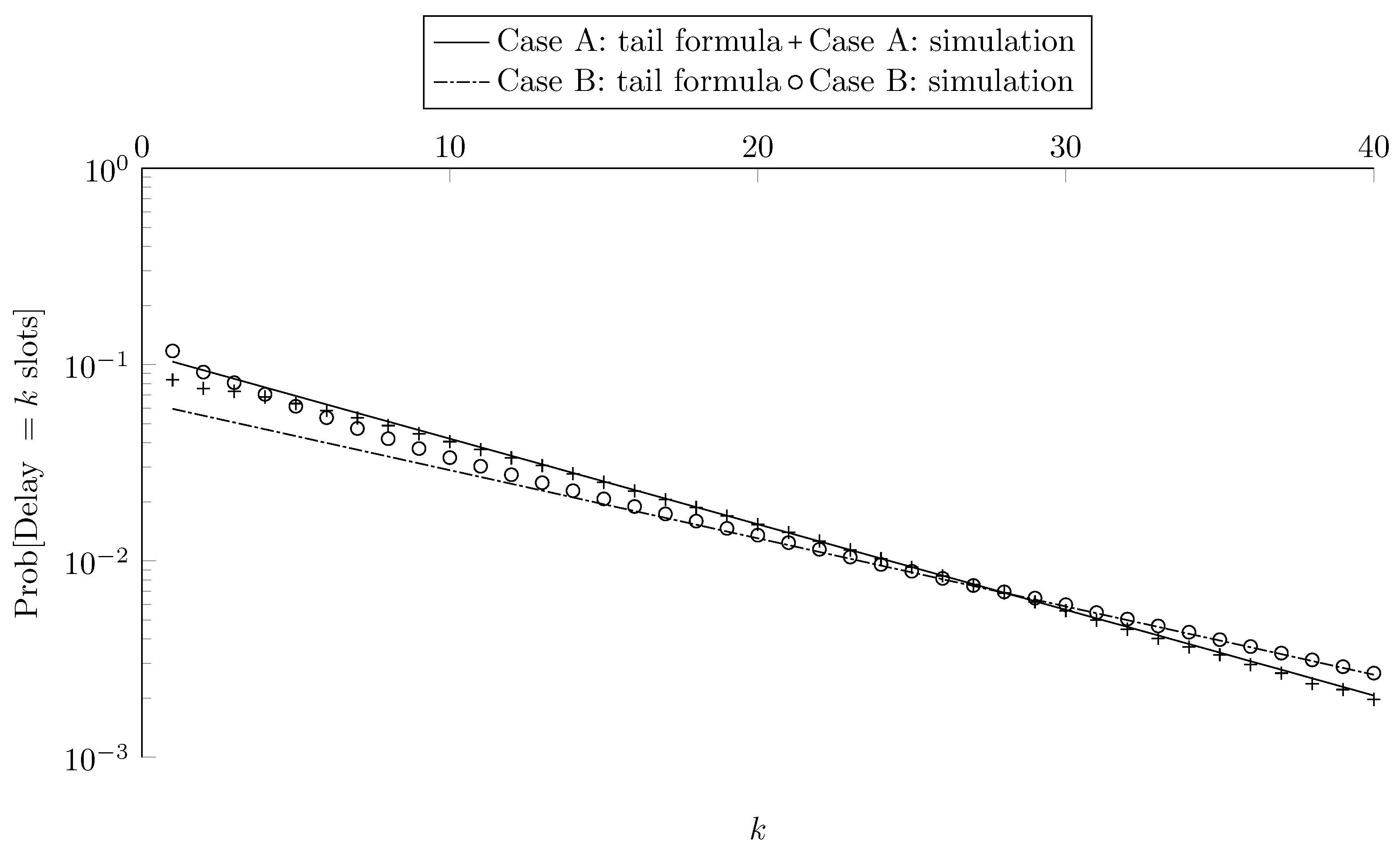
This specific choice for the parameters results in two queueing systems with an equal expected delay of 10.0 slots, which can be obtained using the method of [16] and using Little’s Law [26], and which was also confirmed by simulation. Using the method of the current paper, it can be seen that despite having the same expected delay, and despite being two very similar queueing systems, the tail characteristics of the delay are different, as plotted in Figure 2. We observe that for Case B, there is a larger probability that the delay exceeds a large given value, i.e., the delay distribution of customers has a heavier tail in Case B as compared to Case A.

In the figure the probability mass function of the delay obtained by simulation is also plotted, as a validation of the tail probabilities obtained via the method developed in this paper. For Case A, the results obtained by the method of this paper are within 5% of the results obtained by simulation for $k>8$. For Case B, this is so for $k>17$. The difference between the simulated and calculated results decreases for increasing k, e.g., for Case A the difference is under 1% for $k>15$. The method of this paper thus clearly provides the tail probabilities of the delay with a good accuracy for k sufficiently large. This was verified in several other settings as well, with similar observations on the accuracy. It must be noted that the computational effort to obtain the results by simulation is much higher compared to the method of this paper.

7.2. Influence of Period Lengths

In a second example, we look at the influence of the period lengths on the average delay and 99th percentile. Throughout this subsection, we take the arrival process and the distribution of the period lengths the same for both states, namely a Poisson arrival process with intensity $\lambda$ and a geometrical distribution for the period lengths with parameter $1-\frac{1}{\overline{r}}$ (and thus an expected period length of $\overline{r}$):

$$\begin{array}{cc}\hfill C_1 \left(z\right)& = C_2 \left(z\right) = e^{\lambda (z-1)} ;\hfill \end{array}$$

(76)

$$\begin{array}{cc}\hfill R_1 \left(z\right)& =R_2 \left(z\right) = \frac{z}{\overline{r}-(\overline{r}-1)z} .\hfill \end{array}$$

(77)

For the server availability, we take a fixed number of four servers available per slot in the first state and a fixed number of two servers available per slot in the second state:

$$\begin{array}{c}\hfill S_1 \left(z\right) =z^4 ; S_2 \left(z\right) =z^2 .\end{array}$$

(78)

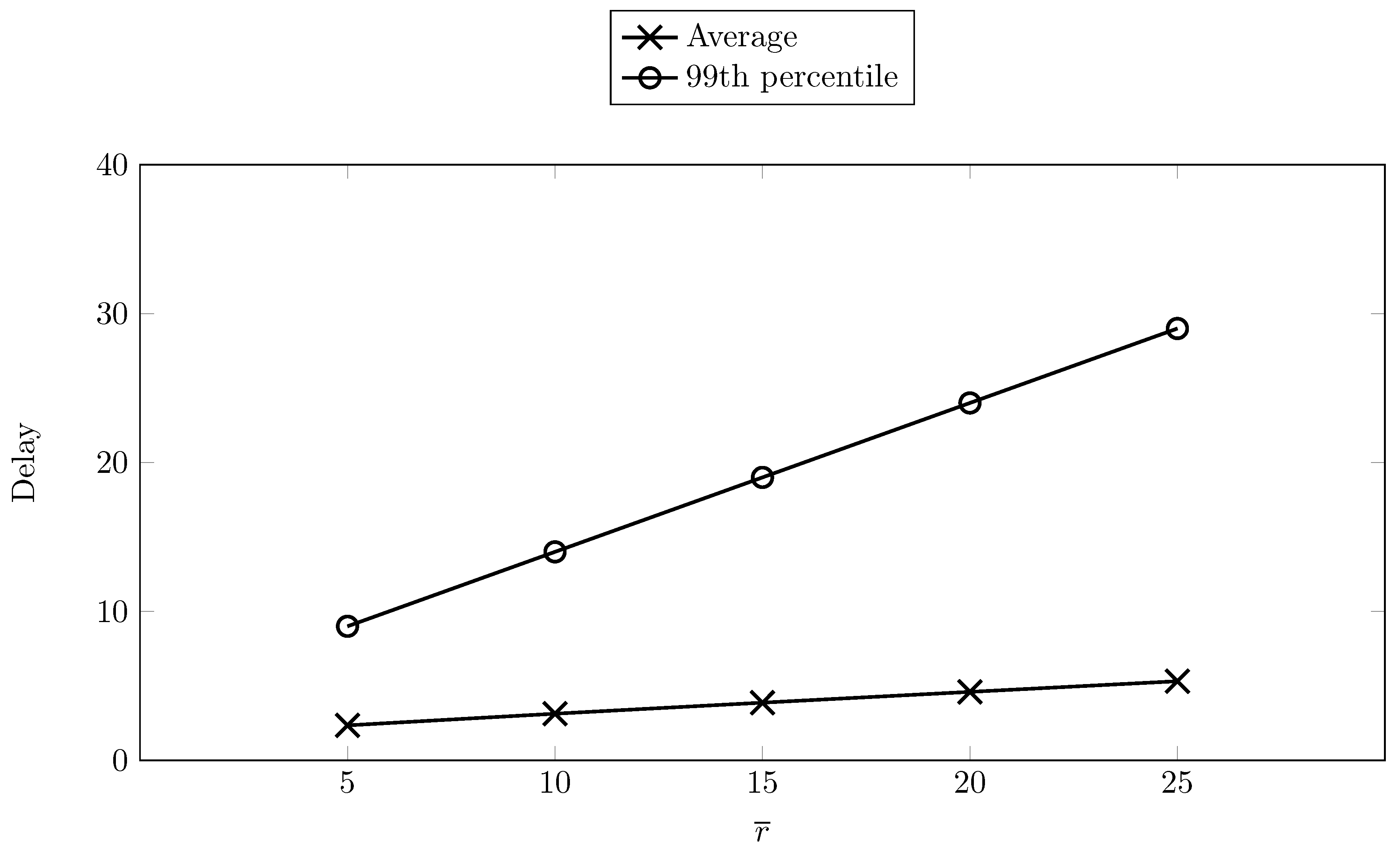
In Figure 3, we plot the average delay and the 99th percentile of the delay in function of the expected period lengths $\overline{r}$ for $\lambda =2.4$. The average delay is calculated from the average system content (as obtained by the method of [16]) by application of Little’s Law [26]. The 99th percentile of the delay, i.e., the smallest k for which $\mathrm{Prob} \left[\mathrm{delay} >k \mathrm{slots}\right]<0.01$, is calculated by inversion of (65):

$$\begin{array}{c}\hfill 99\mathrm{th} \mathrm{percentile} =\mathrm{ceil}\left(-\frac{\ln \left(\frac{0.01·z_0(z_0-1)}{-w_0}\right)}{\ln \left(z_0\right)}\right) .\end{array}$$

(79)

As, on average, there are three servers available, the load is 80%, but in the second state, the system is temporarily overloaded. With increasing period lengths, the average delay increases linearly. This is to be expected as the system remains for longer periods in the overloaded state. The same trend is visible for the 99th percentile of the delay; however, the increase happens with a much steeper slope. This proves that valuable information can be obtained from a tail analysis of the delay. The results of Figure 3 were verified by simulation as well (not plotted as they are not distinguishable from the results obtained by the method of this paper).

7.3. Brief Summary for Implementation

In this subsection, we briefly indicate how the method of this paper can be implemented in order to obtain results such as for the numerical examples given earlier in this section, starting from the pgfs fully describing the queueing system ($R_i \left(z\right)$, $S_i \left(z\right)$ and $C_i \left(z\right)$, as defined in Section 2).

• Numerically obtain the solutions $z_p$ of

  $$\begin{array}{c}\hfill 1-R_1 \left(Y_1 \left(z\right)\right)R_2 \left(Y_2 \left(z\right)\right) =0 \mathrm{for} \left|z\right|\le 1,\end{array}$$

  (80)

  where $Y_i \left(z\right) =C_i \left(z\right)S_i \left(\frac{1}{z}\right)$ and with $z_1=1$. There are a total of $M=m_r^1{m}_s^1+m_r^2{m}_s^2$ such solutions.
• Introduce the functions $Q_i \left(x,z\right)$ according to (18). Calculate the unknowns ${ϵ}_{nj}^i$ by solving the following set of equations for $i=1$ or for $i=2$ (both give an equivalent set of equations):

  $$\begin{array}{c}\hfill S_{\overline{ı}} \left(\frac{1}{z_p}\right)R_{\overline{ı}} \left(Y_{\overline{ı}} \left(z_p\right)\right)\left[Q_i \left(Y_i \left(z_p\right),1\right)-Q_i \left(Y_i \left(z_p\right),\frac{1}{z_p}\right)\right]\\ \hfill \hspace{1em}+S_i \left(\frac{1}{z_p}\right)\left[Q_{\overline{ı}} \left(Y_{\overline{ı}} \left(z_p\right),1\right)-Q_{\overline{ı}} \left(Y_{\overline{ı}} \left(z_p\right),\frac{1}{z_p}\right)\right]=0,& \hspace{1em}p=2\dots M ;\hfill \end{array}$$

  (81)

  $$\begin{array}{cc}\hfill \frac{\frac{\partial }{\partial z}{\left.Q_1 \left(x,z\right)\right|}_{(x,z)=(1,1)}+\frac{\partial }{\partial z}{\left.Q_2 \left(x,z\right)\right|}_{(x,z)=(1,1)}}{{\overline{r}}_1({\overline{s}}_1-{\lambda }_1)+{\overline{r}}_2({\overline{s}}_2-{\lambda }_2)}=1& .\hfill \end{array}$$

  (82)
• Numerically obtain the solutions $x_p$ of

  $$\begin{array}{c}\hfill 1-R_1 \left(Y_1 \left(\frac{1}{x}\right)\right)R_2 \left(Y_2 \left(\frac{1}{x}\right)\right)=0 ; \left|x\right|<1.\end{array}$$

  (83)
• Find $z_0$ as the solution closest to 1 of the following polynomial Equation (for all possible $x_p$):

  $$\begin{array}{c}\hfill g(x_p,z)=0 ,\end{array}$$

  (84)

  with $g \left(x,z\right)$ given in (36) and $x_0$ is then equal to the corresponding $x_p$.
• Fill in the obtained values for $z_0$ and $x_0$ in the expression (67) for $w_0$.

8. Conclusions

In this paper, we have studied the delay characteristics of a discrete-time multiserver queueing model. It is the extension of an earlier work where the system content was treated [16].

The queueing model considers two different system states. Each state is characterized by its own distributions for the number of arrivals and the number of available servers in a slot. Within a state, these numbers are independent and identically distributed random variables. The state transitions occur after stochastic period lengths, and each state has its own distribution for the sojourn time in that state. This setup allows to model a broad variety of queueing systems, where correlations can be introduced in the slot-to-slot arrivals and server availability.

In this paper, we have obtained the tail distribution of the delay for such a queueing model, using a generating functions approach and using the theory of the dominant singularity. Numerical examples have shown the accuracy of the obtained results, and the importance of the work. We have seen that tail characteristics of the delay of a customer in two separate queueing systems can be substantially different even when the systems are very similar and the expected delay is the same. Tail characteristics also provide a further in-depth understanding of the behavior of a queueing system.

References

- Bruneel, H.; Kim, B.G. Discrete-Time Models for Communication Systems Including ATM; Kluwer Academic Publishers Group: Amsterdam, The Netherlands, 1993. [Google Scholar]
- Daigle, J. Queueing Theory with Applications to Packet Telecommunication; Springer Science & Business Media: Berlin/Heidelberg, Germany, 2005. [Google Scholar]
- Alfa, A. Queueing Theory for Telecommunications: Discrete Time Modelling of a Single Node System; Springer Science & Business Media: Berlin/Heidelberg, Germany, 2010. [Google Scholar]
- Kiefer, J.; Wolfowitz, J. On the theory of queues with many servers. Trans. Am. Math. Soc. 1955, 78, 1–18. [Google Scholar] [CrossRef]
- Kim, J.; Kim, B.; Kang, J. Discrete-time multiserver queue with impatient customers. Electron. Lett. 2013, 49, 38–39. [Google Scholar]
- Chaudhry, M.L.; Kim, J.J.; Banik, A.D. Analytically simple and computationally efficient results for the GI(X)/Geo/c queues. J. Probab. Stat. 2019, 2019, 6480139. [Google Scholar] [CrossRef] [Green Version]
- Georganas, N.D. Buffer behavior with Poisson arrivals and bulk geometric service. IEEE Trans. Commun. 1976, 24, 938–940. [Google Scholar] [CrossRef]
- Bruneel, H. A discrete-time queueing system with a stochastic number of servers subjected to random interruptions. Opsearch 1985, 22, 215–231. [Google Scholar]
- Goswami, V.; Mund, G. Computational analysis of multi-server discrete-time queueing system with balking, reneging and synchronous vacations. RAIRO Oper. Res. 2017, 51, 343–358. [Google Scholar] [CrossRef]
- Chaudhry, M.L.; Kim, N.K. A complete and simple solution for a discrete-time multi-server queue with bulk arrivals and deterministic service times. Oper. Res. Lett. 2003, 31, 101–107. [Google Scholar] [CrossRef]
- Bruneel, H.; Steyaert, B.; Desmet, E.; Petit, G. Analytic derivation of tail probabilities for queue lengths and waiting times in ATM multiserver queues. Eur. J. Oper. Res. 1994, 76, 563–572. [Google Scholar] [CrossRef]
- Gao, P.; Wittevrongel, S.; Bruneel, H. Discrete-time multiserver queues with geometric service times. Comput. Oper. Res. 2004, 31, 81–99. [Google Scholar] [CrossRef] [Green Version]
- Laevens, K.; Bruneel, H. Delay analysis for discrete-time queueing systems with multiple randomly interrupted servers. Eur. J. Oper. Res. 1995, 85, 161–177. [Google Scholar] [CrossRef]
- Neuts, M.; Lucantoni, D. A Markovian queue with N servers subject to breakdowns and repair. Manag. Sci. 1979, 25, 849–861. [Google Scholar] [CrossRef]
- De Muynck, M.; Bruneel, H.; Wittevrongel, S. Analysis of a queue with general service demands and correlated service capacities. Ann. Oper. Res. 2020, 293, 73–99. [Google Scholar] [CrossRef]
- Verdonck, F.; Bruneel, H.; Wittevrongel, S. Analysis of a 2-state discrete-time queue with stochastic state-period lengths and state-dependent server availability and arrivals. Perform. Eval. 2019, 135. [Google Scholar] [CrossRef]
- Ibrahim, R.; Whitt, W. Wait-time predictors for customer service systems with time-varying demand and capacity. Oper. Res. 2011, 59, 1106–1118. [Google Scholar] [CrossRef] [Green Version]
- Liu, Y.; Whitt, W. The G t/GI/s t+GI many-server fluid queue. Queueing Syst. 2012, 71, 405–444. [Google Scholar] [CrossRef] [Green Version]
- Grier, N.; Massy, W.; McKoy, T.; Whitt, W. The time-dependent Erlang loss model with retrials. Telecommun. Syst. 1997, 7, 253–265. [Google Scholar] [CrossRef]
- Massey, W. The analysis of queues with time-varying rates for telecommunication models. Telecommun. Syst. 2002, 21, 173–204. [Google Scholar] [CrossRef]
- Wierman, A.; Andrew, L.L.; Tang, A. Power-aware speed scaling in processor sharing systems. In Proceedings of the IEEE INFOCOM, Rio de Janeiro, Brazil, 19–25 April 2009. [Google Scholar]
- Tipper, D.; Yi, Q.; Hou, X. Modeling the time varying behavior of mobile ad hoc networks. In Proceedings of the 7th ACM International Symposium on Modeling, Analysis and Simulation of Wireless and Mobile Systems, Venice, Italy, 4–6 October 2004; pp. 12–19. [Google Scholar]
- Kleinrock, L. Queueing Systems, Volume I: Theory; Wiley: Hoboken, NJ, USA, 1975. [Google Scholar]
- Takagi, H. Queueing Analysis—A Foundation of Performance Evaluation, Volume 3: Discrete-Time Systems; North Holland Amsterdam: Amsterdam, The Netherlands, 1993. [Google Scholar]
- Woodside, C.; Ho, E. Engineering calculation of overflow probabilities in buffers with Markov-interrupted service. IEEE Trans. Commun. 1987, 35, 1272–1277. [Google Scholar] [CrossRef]
- Little, J. A proof for the queueing formula: L = λ W. Oper. Res. 1961, 9, 383–387. [Google Scholar] [CrossRef]
Figure 1.
The delay of customer P.
Figure 2.
Distribution of delay for Case A and Case B both based on the theory of this paper (tail distribution) and based on simulation (probability mass function).
Figure 3.
Average and 99th percentile of the delay for the example of Section 7.2.