Simulations between Three Types of Networks of Splicing Processors

Abstract

Networks of splicing processors (NSP for short) embody a subcategory among the new computational models inspired by natural phenomena with theoretical potential to handle unsolvable problems efficiently. Current literature considers three variants in the context of networks managed by random-context filters. Despite the divergences on system complexity and control degree over the filters, the three variants were proved to hold the same computational power through the simulations of two computationally complete systems: Turing machines and 2-tag systems. However, the conversion between the three models by means of a Turing machine is unattainable because of the huge computational costs incurred. This research paper addresses this issue with the proposal of direct and efficient simulations between the aforementioned paradigms. The information about the nodes and edges (i.e., splicing rules, random-context filters, and connections between nodes) composing any network of splicing processors belonging to one of the three categories is used to design equivalent networks working under the other two models. We demonstrate that these new networks are able to replicate any computational step performed by the original network in a constant number of computational steps and, consequently, we prove that any outcome achieved by the original architecture can be accomplished by the constructed architectures without worsening the time complexity.

1. Introduction

In recent years, the limitations encountered by our standard computational models have become more apparent, motivating the pursuit of knowledge regarding innovative paradigms capable of overcoming these barriers. Along this line of research, different computational models finding their inspiration on natural phenomena have been proposed in the scientific community. Further research showed their theoretical proficiency for solving intractable problems.

Networks of bio-inspired processors are one of such nature-inspired systems under the parallel and distributed computational framework, boasting a high degree of parallelism (theoretically, unlimited). This model shares numerous characteristics with other known computational paradigms of diverse origins: tissue-like P systems [1], which is a model inspired by the tissue structure introduced in the area of membrane computing [2], a model, called evolutionary systems, that is inspired by the evolution of various cell populations [3], networks of parallel language processors, which is a parallel model for generating languages [4], flow-based programming, which is a particular variant of the data-flow programming [5], connection machine, which is a kind of a parallel non-conventional processing computer [6], distributed computing using mobile programs [7], etc.

A network of bio-inspired processors may be informally described as a set of processors that are placed in the vertices of a graph. Each processor acts over data organized in distinct structures: strings, pictures, graphs, multisets, etc. An early survey may be found in [8] and more recently in [9]. Thus far, the literature differentiates between two subcategories of networks of bio-inspired processors handling string data, namely evolutionary and splicing processors. The first one was proposed in [10] as a logical abstraction of the point mutations taking place in DNA sequences: insertion, deletion or substitution of a single base pair. The second category, introduced in [11] and analyzed for its theoretical application for problem solving in [12], mimics the splicing phenomena in DNA molecules overseen by the various restriction and ligase enzymes [13] from a computational point of view. A more general view of restriction enzymes as sources of inspiration for computing can be seen in [14], which opened a wide area of research.

Under this paradigm, the strings hosted in a splicing processor perform the role of DNA molecules, while the behavioral constraints for the splicing enzymes are abstracted to a set of splicing rules composed by quadruples of strings specifying the cutting positions of the strings in the node. Following a splicing operation, the pieces are recombined as long as they are yielded by the same splicing rule. This model shares common aspects with the test tube distributed splicing systems introduced in [15] and posteriorly examined in [16]. The divergences with this last splicing paradigm and time-varying distributed H systems [17] are discussed in [18].

The computation in the networks of splicing processors follows after a sequence of alternative steps, namely splicing and communication, that continues indefinitely until a predefined halting requirement is met. In the splicing step, the strings in each node are simultaneously cut and recombined into new ones according to the constraints set by all the applicable splicing rules of the processor hosted in that node. Thus, each string of the node has enough replications to allow for the synchronous completion of the relevant rules. Next in line, a communication step redistributes the string data in the network as follows:

(i) The string data in a splicing processor is sent to the connected nodes provided that it meets the established exiting conditions for that node.

(ii) The receiving nodes concurrently accept the incoming data satisfying its input requirements. Any string refused by all these nodes is consequently lost.

This data flow in the network is managed through the introduction of random-context filters deciding upon the entering and exiting requirements of the nodes through semantic or syntactical conditions. Thus, far, there are three variants of the latter category: (i) each node is assigned an input and output filter to manage the incoming and exiting string data, respectively, [19], (ii) these two filters are combined into one unique filter [20] and (iii) the filters of two connected nodes are replaced with ones assigned to the edge between them [21].

A simulation of a model by another one is said to preserve the time complexity if the numbers of computational steps performed by the two models on every input are of the same order. It is obvious that (ii) and (iii) are particular variants of (i). Consequently, they appear to offer less control over the computation; however, several works proved they share the same computational power through efficient simulations of known computationally complete models in [11,22,23].

Nevertheless, the indirect conversion between the previous variants through the intermission of a Turing machine is unattainable because of the enormous spike in the complexity. This paper aims to improve upon this line of research with the proposal of efficient direct simulations between the three discussed variants.

2. Basic Definitions

We describe here the basic definitions and nomenclature used for this research. For the remaining notations related to this work, the reader is encouraged to consult [24].

An alphabet refers to a finite and non-empty set of symbols. We write the cardinality of a given finite set S as $card\left(S\right)$. A string over an alphabet V is a finite sequence of symbols belonging to that alphabet V. The set of all strings over the alphabet V is denoted by $V^{*}$, the empty string is expressed by $\epsilon$, and the length of a string z is written $\left|z\right|$. Moreover, $alph\left(z\right)$ is the smallest set $U\subseteq V$ such that $z\in U^{*}$ holds.

A splicing rule over V is a 4-tuple of strings following the structure $[(u_1,u_2);(u_3,u_4)]$, with $u_1,u_2,u_3,u_4\in V^{*}$. Given such a splicing rule $r=[(u_1,u_2);(u_3,u_4)]$ and the strings $\alpha ,\beta \in V^{*}$, we define

$$\begin{array}{ccc}\hfill {\sigma }_r(\alpha ,\beta )& =& \{{\beta }_1{u}_3{u}_2{\alpha }_2\mid \alpha ={\alpha }_1{u}_1{u}_2{\alpha }_2,\beta ={\beta }_1{u}_3{u}_4{\beta }_2,{\alpha }_1,{\alpha }_2,{\beta }_1,{\beta }_2\in V^{*}\}\cup \hfill \\ & & \{{\alpha }_1{u}_1{u}_4{\beta }_2\mid \alpha ={\alpha }_1{u}_1{u}_2{\alpha }_2,\beta ={\beta }_1{u}_3{u}_4{\beta }_2,{\alpha }_1,{\alpha }_2,{\beta }_1,{\beta }_2\in V^{*}\}.\hfill \end{array}$$

This definition may be extended as follows. Given a language L over V and a finite set of splicing rules R, we define

$${\sigma }_R\left(L\right)=\bigcup _{r\in R}\left(\bigcup _{w_1,w_2\in L}{\sigma }_r(w_1,w_2)\right).$$

Given an alphabet V, two disjoint subsets $P,F$ of V, and a string z over V, we define the following predicates:

$${\phi }^{\left(s\right)}(z;P,F)\equiv P\subseteq alph\left(z\right)F\cap alph\left(z\right)=\varnothing$$

$${\phi }^{\left(w\right)}(z;P,F)\equiv alph\left(z\right)\cap P\ne \varnothing F\cap alph\left(z\right)=\varnothing .$$

In these predicates, the set of permitting contexts P defines the symbols that are required to be present in the current string while the set of forbidding contexts F refers to those symbols that are banned. Both clauses require the nonexistence of symbols $a\in F$ in the string z and differ on the flexibility of the conditions related to P. The first one demands for all the symbols in P to exist in z, while the latter statement is met as long as one or more of the symbols in P belong to z.

Given $\beta \in \{w,s\}$ and a language $L\subseteq V^{*}$, we write

$${\phi }^{\beta }(L,P,F)=w\in L\mid {\phi }^{\beta }(w,P,F).$$

A splicing processor with random-context filters (SP) over an alphabet V is a 6-tuple $(S,A,PI,FI,PO,FO)$, where:

–

S is a finite set of splicing rules over V.

–

A is a finite set of strings over V. Each string in A is called an auxiliary string.

–

$PI$ (permitting symbols) and $FI$ (forbidding symbols) are two subsets of V, which both define the input filter of the processor.

–

$PO,FO\subseteq V$ are similar subsets of V that define the output filter of the processor.

We say a splicing processor is uniform if the input and output filters are identical: $PI=PO=P$ and $FI=FO=F$. The set of all splicing processors over the alphabet U is denoted by $S{P}_U$, while $US{P}_U$ denotes the set of all uniform splicing processors over U.

A network of splicing processors (NSP) is a 9-tuple $\Gamma =(V,U,\langle ,\rangle ,G,\mathcal{N},\beta ,\underline{In},\underline{Halt})$, where:

• $V\subset U$ are the input and network alphabet, respectively. The working alphabet U contains two special symbols, namely, $\langle ,\rangle$ that do not belong to V.
• $G=(X_G,E_G)$ is an undirected graph defined by the set $X_G$ of vertices and the set $E_G$ of edges. As the graph does not contain loops, we define an edge by a binary set of vertices. G is called the underlying graph of the network. It is worth mentioning that many papers were dealing with NSP with a complete underlying graph, see, e.g., the survey [9].
• $\mathcal{N}:X_{G}S{P}_U$ is a function that associates with each vertex $x\in X_G$ the splicing processor $\mathcal{N}\left(x\right)=(S_x,A_x,P{I}_x,F{I}_x,P{O}_x,F{O}_x)$.
• $\beta :X_G\{\left(s\right),\left(w\right)\}$ is a function that associates with each vertex the type of both its input and output filters. We now define two mappings on the set of all strings over $U\setminus \{\langle ,\rangle \}$:

  $$\begin{array}{c}\hfill \mathrm{input}\mathrm{filter}:{\rho }_x(.)={\phi }^{\beta \left(x\right)}(.;P{I}_x,F{I}_x).\end{array}$$

  $$\begin{array}{c}\hfill \mathrm{output}\mathrm{filter}:{\tau }_x(.)={\phi }^{\beta \left(x\right)}(.;P{O}_x,F{O}_x).\end{array}$$
  Informally, ${\rho }_x\left(z\right)$ (resp. ${\tau }_x\left(z\right)$) decides whether or not the string z can pass the input (resp. output) filter of x. If L is a language, we define ${\rho }_x\left(L\right)$ by: ${\rho }_x\left(L\right)=\{w\in {(U\setminus \left\{\langle ,\rangle \right\})}^{*}\mid {\rho }_x\left(w\right)\}$, that is the set of strings of L that can pass the input filter of x. In an analogous way, we define ${\tau }_x\left(L\right)$. Note that though we use the same notation for ${\rho }_x\left(w\right)$ (${\tau }_x\left(w\right)$) and ${\rho }_x\left(L\right)$ (${\tau }_x\left(L\right)$), there is no confusion because the arguments are different.
• $\underline{In},\underline{Halt}\in X_G$ are the input and the halting node of $\Gamma$, respectively.

Likewise, a network of splicing processors is considered to be uniform if it is composed by uniform splicing processors. A network of uniform splicing processors (NUSP) is a 9-tuple $\Gamma =(V,U,\langle ,\rangle ,G,\mathcal{N},\beta ,\underline{In},\underline{Halt})$,where:

• $V,U,\langle ,\rangle ,G,\underline{In},\underline{Halt}$ follow the same specifications as the parameters in NSP.
• $\mathcal{N}:X_{G}US{P}_U$ is a function that returns the uniform splicing processor $\mathcal{N}\left(x\right)=(S_x,A_x,P_x,F_x)$ associated with the node $x\in X_G$.
• $\beta :X_G\{\left(s\right),\left(w\right)\}$ specifies the strength of the sets P and F associated to node filters.

A network of splicing processors with filtered connections (NSPFC) is a 9-tuple $\Gamma =(V,U,\langle ,\rangle ,G,\mathcal{N},\beta ,\underline{In},\underline{Halt})$, where:

• $V,U,\langle ,\rangle ,\underline{In},\underline{Halt}$ follow the same specifications as the parameters in NSP.
• $G=(X_G,E_G)$ is also an undirected graph such that each node $x\in X_G$ is seen as a splicing processor without filters, with the set of splicing rules $S_x$ and the set of axioms $A_x$.
• $\mathcal{N}:E_G{2}^U\times 2^U$ associates with each edge $e\in E_G$ a pair of sets $P_e,F_e$ that define the filter on the edge e.
• $\beta :E_G\{\left(s\right),\left(w\right)\}$ defines the predicate variant assigned to the edge filters.

The size of a NSP $\Gamma$ belonging to any of the variants above is defined as the number of nodes in the graph, i.e., $card\left(X_G\right)$. A configuration of $\Gamma$ is a mapping $C:X_G⟶2^{U^{*}}$, which assigns a set of strings $C\left(x\right)$ to each node $x\in \Gamma$, that is the sets of strings that can be found in node x at a given moment. Although for each $x\in X_G$, $C\left(x\right)$ is actually a multiset of strings, each string appearing in an arbitrary number of copies, for the sake of simplicity, we work with the support of this multiset. For a string $z\in V^{*}$, the initial configuration of $\Gamma$ on the input string z is $C_0^{\left(z\right)}\left(\underline{In}\right)=\left\{\langle z\rangle \right\}$ and $C_0^{\left(z\right)}\left(x\right)=\varnothing$ for all $x\in X_G\setminus \underline{In}$.

A configuration can be altered through a splicing step or a communication step. In a splicing step, all the splicing rules belonging to the set $S_x$ applicable to the strings in the set combination of $C\left(x\right)$ and $A_x$ are realized, causing the change of C to a new configuration $C^{\prime }$. Formally, a configuration C evolves to $C^{\prime }$ by a splicing step, denoted as $C⟹C^{\prime }$, if and only if the following proposition is true for all $x\in X_G$:

$$C^{\prime }\left(x\right)={\sigma }_{S_x}(C\left(x\right)\cup A_x).$$

The communication step is different in NSP (NUSP) and NSPFC. We first define how a communication step works in a NSP (the definition of a communication step in a NUSP is very similar, hence left to the reader). In every node x, all the following tasks are accomplished simultaneously:

(i)

The strings that satisfy the output filter condition of x are sent out;

(ii)

Copies of the expelled strings from any node y connected to x enter x, provided that they satisfy the input filter condition of x.

We stress that those strings sent out of x that do not satisfy the input filter condition of any node are definitely lost. Formally, a configuration $C^{\prime }$ follows a configuration C by a communication step in a NSP (we write $C^{\prime }\vDash C)$ if for all $x\in X_G$

$$C^{\prime }\left(x\right)=(C\left(x\right)-{\phi }^{\beta \left(x\right)}(C\left(x\right),P{O}_x,F{O}_x))\cup$$

$${\displaystyle \bigcup _{\{x,y\}\in E_G}({\phi }^{\beta \left(y\right)}(C\left(y\right),P{O}_y,F{O}_y)\cap {\phi }^{\beta \left(x\right)}(C\left(y\right),P{I}_x,F{I}_x))}$$

holds.

We now describe how a communication step works in a NSPFC. For every pair of connected nodes $x,y$, all the strings that satisfy the filter condition associated with the edge $\{x,y\}$ are moved from one node to the other. Formally, $C⊢C^{\prime }$, if

$$C^{\prime }(x)=(C(x)\setminus (\bigcup _{\{x,y\}\in E_G}{\phi }^{\beta (\{x,y\})}(C(x),\mathcal{N}(\{x,y\}))))$$

$$\cup (\bigcup _{\{x,y\}\in E_G}{\phi }^{\beta \left(\right\{x,y\left\}\right)}(C\left(y\right),\mathcal{N}\left(\{x,y\}\right)))$$

for all $x\in X_G.$

The computation of a NSP $\Gamma$ on the input string $w\in V^{*}$ is defined as a sequence of alternating steps (splicing, communication) that produces the configurations $C_0^{\left(w\right)}$, $C_1^{\left(w\right)}$, $C_2^{\left(w\right)},\cdots$, such that $C_{2i}^{\left(w\right)}⟹C_{2i+1}^{\left(w\right)}$ and $C_{2i+1}^{\left(w\right)}\vDash C_{2i+2}^{\left(w\right)}$, for all $i\ge 0$. The computation of NUSP and NSPFC are defined in the same way.

A computation as above halts, if there exists $k\ge 1$ such that the set of strings existing in the output node $C\left(\underline{Halt}\right)$ is non-empty. Then, we say that the string w is admitted by the splicing network in an accepting computation. The language defined/accepted by $\Gamma$ is the set of all strings w over V such that the computation of $\Gamma$ on w is an accepting one.

The time complexity of the halting computation $C_0^{\left(x\right)}$, $C_1^{\left(x\right)}$, $C_2^{\left(x\right)}$, $\cdots C_m^{\left(x\right)}$ of $\Gamma$ on $x\in V^{*}$ is denoted by $tim{e}_{\Gamma }\left(x\right)$ and equals m. The time complexity of $\Gamma$ is the partial function from $IN$ to $IN$ formalized as follows:

$$Tim{e}_{\Gamma }\left(n\right)=\max \{Tim{e}_{\Gamma }\left(x\right)\mid x\in L(\Gamma ),\left|x\right|=n\}.$$

Furthermore, for a function $f:IN\to IN$ and we write

$${\mathbf{Time}}_{NSP}\left(f\left(n\right)\right)=\{L\mid L \mathrm{is} \mathrm{accepted} \mathrm{by} \mathrm{a} \mathrm{NSP}\Gamma \mathrm{such} \mathrm{that}Tim{e}_{\Gamma }\left(n\right)\in \mathcal{O}\left(f\left(n\right)\right)\}.$$

Analogously, one defines ${\mathbf{Time}}_{NUSP}\left(f\left(n\right)\right)$ as well as ${\mathbf{Time}}_{NSPFC}\left(f\left(n\right)\right)$.

3. Direct Simulations between NSPs and NUSPs

Obviously, since each NUSP can be immediately transformed into a NSP, we have:

Proposition 1. 

${\mathbf{Time}}_{NUSP}\left(f\left(n\right)\right)\subseteq {\mathbf{Time}}_{NSP}\left(f\left(n\right)\right)$ for any function $f:IN\to IN$.

The converse is also true, namely:

Proposition 2. 

${\mathbf{Time}}_{NSP}\left(f\left(n\right)\right)\subseteq {\mathbf{Time}}_{NUSP}\left(f\left(n\right)\right)$ for any function $f:IN\to IN$.

Proof. 

Let $\Gamma =(V,U,<,>,G,\mathcal{N},\beta ,x_1,x_n)$ be a NSP with the underlying graph $G=(X_G,E_G)$ and $X_G=\{x_1,x_2,\cdots ,x_n\}$ for some $n\ge 1$; $x_1\equiv \underline{In}$ and $x_n\equiv \underline{Halt}$. Let further $dom\left(S_{x_i}\right)=\{a,b,u,v\in U*\mid [(a,b);(u,v)]\in S_{x_i}\}$. We construct the NUSP ${\Gamma }^{\prime }=(V^{\prime },U^{\prime },<,>,G^{\prime },{\mathcal{N}}^{\prime },{\beta }^{\prime },x_1^s,x_n^s)$; $x_1^s\equiv \underline{In}$ and $x_n^s\equiv \underline{Halt}$, where

$U^{\prime }=U\cup U_{▼}\cup T$,	$U_{▼}=\{a_{▼}\mid a\in U\}$,
$T=\{\#,\psi \}\cup \{{\$}_i,{\#}_i,{\theta }_i,{\yen }_i\mid 1\le i\le n\}$,	$V^{\prime }=V$,
$u_{▼}=a_{▼}^1{a}_{▼}^2\cdots a_{▼}^{\left|u\right|}\mid u=a^1{a}^2\cdots a^{\left|u\right|}\in U^{*}$,	$z_{▼}(u,v)={\beta }_1{u}_{▼}{v}_{▼}{\beta }_2\mid z={\beta }_{1}uvs.{\beta }_2\in U^{*}$

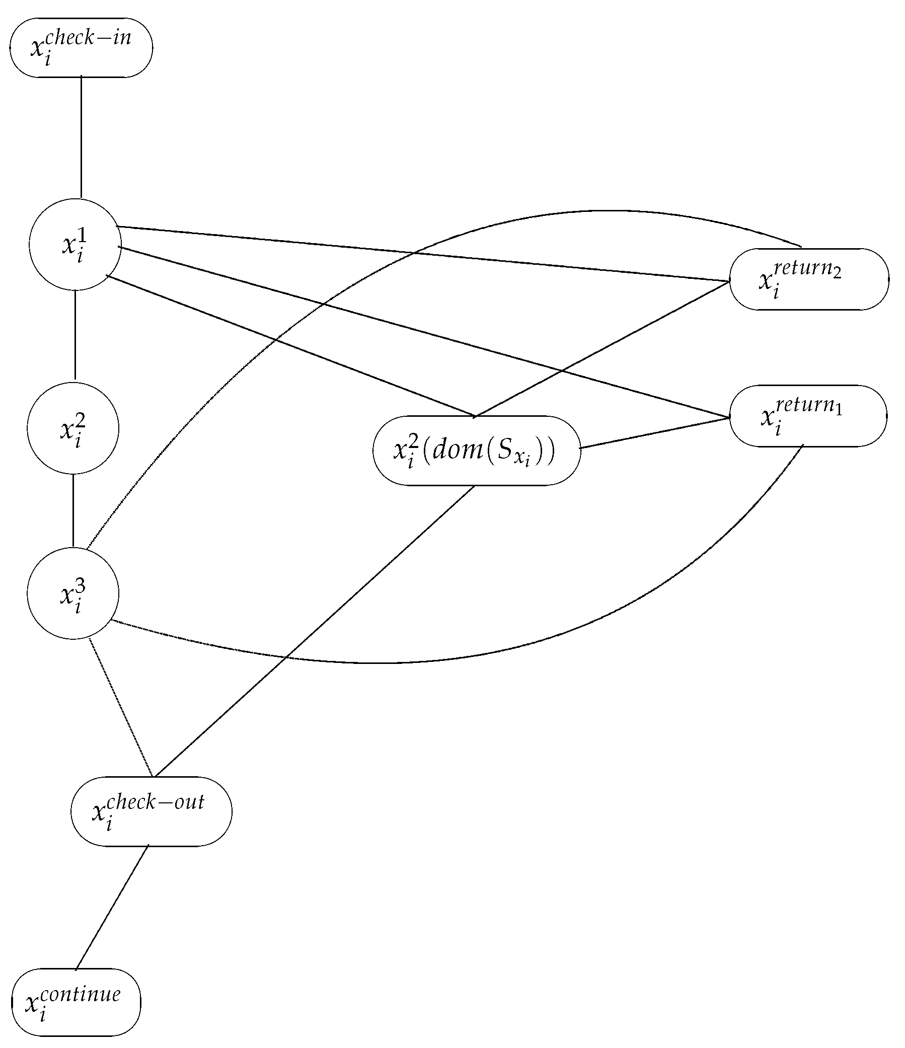
We now define the nodes of $G^{\prime }$ by

Table 1. Description of the initial nodes.

Node	S	P	F	A	${\mathit{\beta }}^{\prime }$
$x_1^s$	$\left\{\right[(\epsilon ,>);(\#,\psi >)\left]\right\}$	$\{\varnothing \}$	$\{\#,{\#}_1,{\theta }_1\}$	$\{\#\psi >\}$	$\left(s\right)$
$x_1^0$	$\left\{[(\epsilon ,\psi >);(\#,>{\#}_1)]\right\}\cup$	$\{\varnothing \}$	$(U_{▼}\cup T)\setminus \{>,{\#}_1\}$	$\{\#>{\#}_1,\#{\theta }_1\}$	$\left(s\right)$
$x_1^0$	$\left\{[(\epsilon ,\psi >);(\#,>{\#}_1)]\right\}\cup$	$\{\varnothing \}$	$(U_{▼}\cup T)\setminus \{>,{\#}_1\}$	$\{\#>{\#}_1,\#{\theta }_1\}$	$\left(s\right)$
	$\left\{[(\epsilon ,{\#}_1);(\#,{\theta }_1)]\right\}$

,

Table 2. Description of the intermediate nodes.

Node	S	P	F	A	${\mathit{\beta }}^{\prime }$
$x_i^{check-in}$	$\left\{[(\epsilon ,{\$}_i);(\#,{\#}_i)]\right\}$	$P{I}_{x_i}$	$(F{I}_{x_i}\cup U_{▼}\cup T)\setminus$	$\{\#{\#}_i,\#{\theta }_i\}$	$\beta \left(x_i\right)$
	$\left\{[(\epsilon ,{\#}_i);(\#,{\theta }_i)]\right\}$		$\{{\$}_i,{\#}_i\}$
$x_i^1$	$\left\{\right\{[(a,b);(u_{▼},v_{▼})]\mid$	$\left\{{\#}_i\right\}$	$\{{\theta }_i,\#\}$	$\{{z^k}_{▼}(u,v){\#}_i\mid$	$\left(s\right)$
	$[(a,b);(u,v)]\in S_{x_i}\}$			$1\le k\le card\left(A_{x_i}\right),$
				$z^k\in A_{x_i}\}$
$x_i^2$	$\left\{[(\epsilon ,{\#}_i);(\#,{\theta }_i)]\right\}$	$U_{▼}$	$T\setminus \{{\theta }_i,{\#}_i\}$	$\{\#{\theta }_i\}$	$\left(w\right)$
$x_i^2\left(dom\left(S_{x_i}\right)\right),$	$\left\{[(\epsilon ,{\#}_i);(\#,{\theta }_i)]\right\}$	$\{{\theta }_i,{\#}_i\}$	$(dom\left(S_{x_i}\right)\cup T\cup U_{▼})\setminus$	$\{\#{\theta }_i\}$	$\left(w\right)$
			$\{{\theta }_i,{\#}_i\}$
$x_i^3$	$\{[(u_{▼},b);(\pi u,\#)]\mid$	$\left\{{\theta }_i\right\}$	$\{\#,\pi \}$	$\{\pi u\#,\#v\pi {\theta }_i\}$	$\left(s\right)$
	$b\in \{U^{*}\cup \left\{{\theta }_i\right\}\}\}\cup$
	$\{[(\pi ,ub);(t,u_{▼}\#)]\mid \{u,t\}\in U^{*},$
	$b\in \{U^{*}\cup \left\{{\theta }_i\right\}\}\}\cup$
	$\{[(a,v_{▼});(\#,vs.\pi )]\mid a\in U^{*}\}\cup$
	$\{[(av,\pi );(\#v_{▼},t)]\mid \{a,v\}\in U^{*},$
	$t\in U^{*}\cup \left\{{\theta }_i\right\}\}$
$x_i^{check-out}$	$\left\{[(\epsilon ,{\theta }_i);(\#,{\yen }_i)]\right\}$	$P{O}_{x_i}$	$F{O}_{x_i}\cup U_{▼}\cup$	$\{\#{\yen }_i\}$	$\beta \left(x_i\right)$
			$(T\setminus \{{\theta }_i,{\yen }_i\})$
$x_i^{continue}$	$\{[(\epsilon ,{\yen }_i);(\#,{\$}_j)]\mid$	∅	$T\setminus (\left\{{\yen }_i\right\}\cup \{{\$}_j\mid$	$\{\#{\$}_j\}$	$\left(s\right)$
	$\{x_i,x_j\}\in E_G\}$		$\{x_i,x_j\}\in E_G\left\}\right)$
$x_i^{retur{n}_1}$	$\left\{[(\epsilon ,{\theta }_i);(\#,{\#}_i)]\right\}$	$F{O}_{x_i}$	$U_{▼}\cup \{\#,{\$}_j,{\yen }_j\mid$	$\{\#{\#}_i\}$	$\left(w\right)$
			$1\le j\le n\}$
$x_i^{retur{n}_2}$	$\left\{[(\epsilon ,{\theta }_i);(\#,{\#}_i)]\right\}$	∅	$P{O}_{x_i}\cup \{\#,{\$}_j,{\yen }_j\mid$	$\{\#{\#}_i\}$	$\left(s\right)$
			$1\le j\le n\}\cup U_{▼}$

and

Table 3. Description of the returning nodes.

Node	S	P	F	A	${\mathit{\beta }}^{\prime }$
$x_i^{retur{n}_2^k}$	$\left\{[(\epsilon ,{\theta }_i);(\#,{\#}_i)]\right\}$	∅	$\left\{Z_k\right\}\cup U_{▼}\cup$	$\{\#{\#}_i\}$	$\left(w\right)$
			$\{\#,{\$}_j,{\yen }_j\mid 1\le j\le n\}$

, while the edges of $G^{\prime }$ are both listed as well as graphically represented.

and $\{x_1^s,x_1^0\},\{x_1^0,x_1^1\}\in E_{G^{\prime }}.$

Let $x_i$, $1\le i\le n-1$ be a splicing node. If $\beta \left(x_i\right)=\left(w\right)$, then the nodes defined in Table 2 belong to $X_{G^{\prime }}$.

All the edges

 – $\{x_1^s,x_1^0\}$,

 – $\{x_1^0,x_1^1\}$,

 – $\{x_i^{check-in},x_i^1\}$ for $1\le i\le n-1$,

 – $\{x_i^1,x_i^2\}$, $\{x_i^1,x_i^2\left(dom\left(S_{x_i}\right)\right)\}$ for $1\le i\le n-1$,

 – $\{x_i^1,x_i^{retur{n}_1}\}$, $\{x_i^1,x_i^{retur{n}_2}\}$ for $1\le i\le n-1$,

 – $\{x_i^2,x_i^3\}$ for $1\le i\le n-1$,

 – $\{x_i^3,x_i^{check-out}\}$, $\{x_i^3,x_i^{retur{n}_1}\}$, $\{x_i^3,x_i^{retur{n}_2}\}$

  for $1\le i\le n-1$,

 – $\{x_i^{check-out},x_i^{continue}\}$, $\{x_i^{check-out},x_i^2\left(dom\left(S_{x_i}\right)\right)\}$

  for $1\le i\le n-1$,

 – $\{x_i^{continue},x_j^{check-in}\}$ for all $\{x_i,x_j\}\in E_G$, $1\le i\ne j\le n-1$,

 – $\{x_i^2\left(dom\left(S_{x_i}\right)\right),x_i^{retur{n}_1}\}$, $\{x_i^2\left(dom\left(S_{x_i}\right)\right),x_i^{retur{n}_2}\}$ for $1\le i\le n-1$,

belong to $E_{G^{\prime }}$. As we have mentioned above, we present also a graphical representation in Figure 1.

If $\beta \left(x_i\right)=\left(s\right)$, then $x_i^{retur{n}_2}$ is replaced by $p\ge 1$ nodes of the form $x_i^{retur{n}_2^k}$, $1\le k\le p$, where $P{O}_{x_i}=\{Z_1,Z_2,\cdots ,Z_p\}$, $p\ge 1$. They are presented in Table 3. Furthermore, if $P{O}_{x_i}=\varnothing$, then $x_i^{retur{n}_2}$ is removed. Analogously, if $F{O}_{x_i}=\varnothing$, then $x_i^{retur{n}_1}$ is removed. Now, an edge between $x_i^1$, $x_i^3$ and $x_i^2\left(dom\left(S_{x_i}\right)\right)$, $[(a,b);(u,v)]\in dom\left(S_{x_i}\right)$, on the one hand, and each node $x_i^{retur{n}_2^k}$, on the other hand, is added to $E_{G^{\prime }}$.

The output node $x_n^s$ is defined as follows: $S^{\prime }\left(x_n^s\right)=S\left(x_n\right)$, $P^{\prime }\left(x_n^s\right)=PI\left(x_n\right)$ and $F^{\prime }\left(x_n^s\right)=FI\left(x_n\right)$, with $A^{\prime }\left(x_n^s\right)=A\left(x_n\right)$, ${\beta }^{\prime }\left(x_n^s\right)=\beta \left(x_n\right)$. Finally, we add all the edges $\{x_i^{continue},x_n^s\}\mid x_i,x_n\in E_G$, to $E_{G^{\prime }}$.

We now analyze a computation of ${\Gamma }^{\prime }$ on an input string $<w>$. In the input node $x_1^s$, > is replaced with the sequence $\psi >$. Then, $<w\psi >$ enters $x_1^0$, where $\psi >$ is replaced with the symbols $>{\#}_1$ and the resulting string is sent to the node $x_1^1$. Thus, the node $x_1^1$ contains the string $z^{\prime }=<w>{\#}_1$ associated to the input string $z=<w>$ placed in the node $x_1\in \Gamma$. More generally, we may assume that a string $w^{\prime }=z_1{z}_2{\#}_i$, for some $1\le i\le n-1$, is in $x_i^1$ if $x_i\in X_G$ contains the corresponding string $w=z_1{z}_2\in U^{*}$. Note that any string produced in $x_1^1$ can return to $x_1^0$. However, these strings have the character ${\#}_1$ switched with ${\theta }_1$, which is not accepted by the connected nodes $x_1^s$ and $x_1^1$. Consequently, the node $x_1^0$ can be disregarded for the rest of the computation.

We now start the simulation of the first splicing step executed by $\Gamma$.

Firstly, we analyze the procedure for the case of a splicing node $x_i\in \Gamma$. In $x_i^1$, a rule $[(a,b);(u_{▼},v_{▼})]$ is applied to $z_1{z}_2{\#}_i$ producing ${\alpha }_{1}a{v}_{▼}{\beta }_2$ and ${\beta }_1{u}_{▼}b{\alpha }_2$, if a rule $\left[\right(a,b);(u,v\left)\right]$ can be applied to $z_1{z}_2$ in the node $x_i\in X_G$. Let $y_1{y}_2{\#}_i$ be one string obtained after a splicing step from $z_1{z}_2{\#}_i$ in $x_i^1$. Note that if the splicing rule cannot be applied, then $z_1{z}_2{\#}_i$ may go out from $x_i^1$ and enter the following nodes:

• $x_i^{check-in}$, provided that $z_1{z}_2$ satisfies the condition of the input filter of $x_i\in X_G$,
• $x_i^{retur{n}_1}$ and $x_i^{retur{n}_2}$ if $\beta \left(x_i\right)=\left(w\right)$ or each of the nodes $x_i^{retur{n}_2^k}$ if $\beta \left(x_i\right)=\left(s\right)$, provided that $z_1{z}_2$ does not satisfy the condition of the output filter of $x_i\in X_G$,
• $x_i^2\left(dom\left(S_{x_i}\right)\right)$.

All cases are to be analyzed. If $z_1{z}_2{\#}_i$ leaves $x_i^1$ and enters $x_i^{check-in}$, the symbol ${\#}_i$ is replaced with ${\theta }_i$, which locks the string in that node. If $z_1{z}_2{\#}_i$ leaves $x_i^1$ and enters $x_i^{retur{n}_1}$, then ping-pong processes between these two nodes as well as between $x_i^1$ and $x_i^2\left(dom\left(S_{x_i}\right)\right)$ start. We distinguish here the cases of weak and strong filters. If $\beta \left(x_i\right)=\left(w\right)$, the string $z_1{z}_2{\#}_i$ can also enter $x_i^{retur{n}_2}$, starting an identical relationship to the one between $x_i^{retur{n}_1}$ and the nodes $x_i^1$, $x_i^2\left(dom\left(S_{x_i}\right)\right)$. If $\beta \left(x_i\right)=\left(s\right)$, the string enters the nodes $x_i^{retur{n}_2^k}$, provided that $z_1{z}_2{\#}_i$ does not contain the character $Z_k$, followed by the same ping-pong process between these nodes and $x_i^1$, $x_i^2\left(dom\left(S_{x_i}\right)\right)$. In this last case, the structure simulates the situation where a string remains in the node $x_i$ because it only contains a proper subset of the characters in $PO\left(x_i\right)$.

If $z_1{z}_2{\#}_i$ leaves $x_i^1$ and enters $x_i^2\left(dom\left(S_{x_i}\right)\right)$, then ${\#}_i$ is replaced by ${\theta }_i$; the new string $z_1{z}_2{\theta }_i$ is simultaneously sent to all nodes $x_i^{check-out}$, $x_i^{retur{n}_1}$ and $x_i^{retur{n}_2}$. If it enters $x_i^{check-out}$, then ${\theta }_i$ is replaced firstly by ${\yen }_i$ (in $x_i^{check-out}$) and secondly by some ${\$}_j$ (in $x_i^{continue}$) provided that $\{x_i,x_j\}\in E_G$. The newly obtained string $z_1{z}_2{\$}_j$ is sent to $x_j^{check-in}$. Note that this situation simulates exactly the situation when $z_1{z}_2$ is sent to $x_j$ after staying unchanged for one splicing step in $x_i$. The case when $z_1{z}_2{\theta }_i$ enters any of the nodes $x_i^{retur{n}_1}$ and $x_i^{retur{n}_2}$ is considered above.

The only case remaining to be analyzed is when $z_1{z}_2{\#}_i$ is transformed into $y_1{y}_2{\#}_i$ (either $y_1=z_1$ or $y_2=z_2$) after applying a splicing rule in $x_i^1$. Then, $y_1{y}_2{\#}_i$ leaves $x_i^1$. We follow the route of this string through the network: $x_i^2$, where ${\#}_i$ is replaced by ${\theta }_i$, then $x_i^3$, where $u_{▼}$ and $v_{▼}$ are replaced by u and v, respectively. We analyze in detail the case for a string $y_1{y}_2{\theta }_i$ with $y_1\ne z_1$. The application of the first splicing rule on a string $y={\beta }_1{u}_{▼}{y}_2{\theta }_i$ yields two strings, namely $y^{\prime }={\beta }_1{u}_{▼}\#$ and $y^{\prime \prime }=\pi u{y}_2{\theta }_i$. These two strings cannot exit the node, as they contain # and $\pi$, respectively. In the next splicing step, these two strings can only combine between themselves through the second splicing rule $\{[(\pi ,ub);(t,u_{▼}\#)]$, yielding two new strings: ${y^{\prime }}^2=\pi u_{▼}\#$ and ${y^{\prime \prime }}^2={\beta }_{1}u{y}_2{\theta }_i$. The first one cannot be used in the computation anymore, while the latter is the original string $y_1{y}_2{\theta }_i$ with $u_{▼}$ replaced by u. The procedure for a string $y_1{y}_2{\theta }_i$ with $y_2\ne z_2$ is analogous through the application of the other two splicing rules.

After leaving $x_i^3$, the new string, say $z^{\prime }$, can enter either $x_i^{check-out}$ or at least one of $x_i^{retur{n}_1}$ and $x_i^{retur{n}_2}$. If it enters $x_i^{check-out}$ and consequently $x_i^{continue}$, then the following computational step in $\Gamma$ was simulated in ${\Gamma }^{\prime }$ as follows: $z^{\prime }$ was obtained from $z_1{z}_2$ by means of a splicing rule $\left[\right(a,b);(u,v\left)\right]$ in $x_i\in X_G$, then $z^{\prime }$ was sent to all neighbors of $x_i$. The situation when $z^{\prime }$ enters one of the nodes $x_i^{retur{n}_1}$ and $x_i^{retur{n}_2}$ corresponds to the situation when $z^{\prime }$ remains in $x_i$ for a new splicing step, as it cannot pass the output filter of $x_i$.

We now analyze the computational steps required for simulating a computation in $\Gamma$. The input node $x_1^s$ and $x_1^0$ require 1 splicing step (or 2 computational steps) each. In the worst case, a splicing step in one of the nodes $\{x_i\mid 1\le i\le n-1\}$ can be simulated in ${\Gamma }^{\prime }$ in 7 splicing steps (or 14 computational steps) distributed in the following way:

• 2 steps in $x_i^1$.
• 2 steps in $x_i^2$.
• 4 steps in $x_i^3$.
• 2 steps in $x_i^{check-out}$.
• 2 steps in $x_i^{continue}$.
• 2 steps in $x_j^{check-in}$$\mid 1\le j\le n-1$.

Note that the simulation only requires 12 computational steps if $x_j\equiv x_n^s$ since $x_n^s$ is not simulated by a subnetwork and the computation halts once a string enters that node. By all the above considerations, we conclude that $L(\Gamma )=L\left({\Gamma }^{\prime }\right)$ and $Tim{e}_{{\Gamma }^{\prime }}\left(n\right)\in \mathcal{O}\left(Tim{e}_{\Gamma }\left(n\right)\right)$. □

4. Direct Simulations between NSPs and NSPFCs

Proposition 3. 

${\mathbf{Time}}_{NSP}\left(f\left(n\right)\right)\subseteq {\mathbf{Time}}_{NSPFC}\left(f\left(n\right)\right)$ for any function $f:$.

Proof. 

We take a NSP $\Gamma =(V,U,<,>,G,\mathcal{N},\beta ,x_1,x_n)$ with the underlying graph $G=(X_G,E_G)$ with the set of nodes $X_G=\{x_1,x_2,\cdots ,x_n\}$ for some $n\ge 1$; $x_1\equiv \underline{In}$ and $x_n\equiv \underline{Halt}$. We construct the NSPFC ${\Gamma }^{\prime }=(V^{\prime },U^{\prime },<,>,G^{\prime },{\mathcal{N}}^{\prime },{\beta }^{\prime },x_I,x_n^s)$; $x_I\equiv \underline{In}$ and $x_n^s\equiv \underline{Halt}$, where

$V^{\prime }=V$,	$U^{\prime }=U\cup U_{▼}\cup T$,
$U_{▼}=\{a_{▼}\mid a\in U\}$,	$u_{▼}=a_{▼}^1{a}_{▼}^2\cdots a_{▼}^{\left|u\right|}\mid u=a^1{a}^2\cdots a^{\left|u\right|}\in U^{*}$,
$z_{▼}(u,v)={\beta }_1{u}_{▼}{v}_{▼}{\beta }_2\mid z={\beta }_{1}uvs.{\beta }_2\in U^{*}$,	$T=\{{\$}_i\mid i\in \{1,\dots ,n\}\}\cup \{\#,\$,\pi ,\theta ,\sigma \}$

We now define the parameters of ${\Gamma }^{\prime }$. First, for each pair of nodes $x_i,x_j\mid 1\le i\ne j\le n,i\ne n$ of $X_G$ with $\{x_i,x_j\}\in E_G$, we have the following nodes in ${\Gamma }^{\prime }$

$x_{i,j}^1$:	$S(x_{i,j}^1)=\left\{[(\epsilon ,\theta );(\#,\$)]\right\}$,	$A\left(x_{i,j}^1\right)=\{\#\$\}$,
$x_{i,j}^2$:	$S(x_{i,j}^2)=\left\{[(\epsilon ,\$);(\#,\psi )]\right\}$,	$A\left(x_{i,j}^2\right)=\{\#\psi \}$,

and the following edges (the nodes $x_i^f$ and $x_j^s$ are to be defined below):

$\{x_i^f,x_{i,j}^1\}$:	$P=PO\left(x_i\right)$,	$F=FO\left(x_i\right)\cup \left\{\$\right\}$,	${\beta }^{\prime }=\beta \left(x_i\right)$,
$\{x_{i,j}^1,x_{i,j}^2\}$:	$P=\left\{\$\right\}$,	$F=\left\{\psi \right\}$,	${\beta }^{\prime }=\left(w\right)$,
$\{x_{i,j}^2,x_j^s\}$:	$P=PI\left(x_j\right)$,	$F=FI\left(x_j\right)\cup \{\$,{\$}_j,\theta \}$,	${\beta }^{\prime }=\beta \left(x_j\right)$.

The specifications for the input node $x_I$ and the output node $x_n^s$ are as follows:

$x_I$:	$S\left(x_I\right)=\left\{[(\epsilon ,>);(\#,>\psi )]\right\}$,	$A\left(x_I\right)=\{\#>\psi \}$,
$x_n^s$:	$S\left(x_n^s\right)=S(x_n\in \Gamma )$,	$A\left(x_n^s\right)=A(x_n\in \Gamma )$.

and the edge:

$\{x_I,x_1^s\}$:

$P=\left\{\psi \right\}$,

$F=\{\#\}$,

${\beta }^{\prime }=\left(s\right)$.

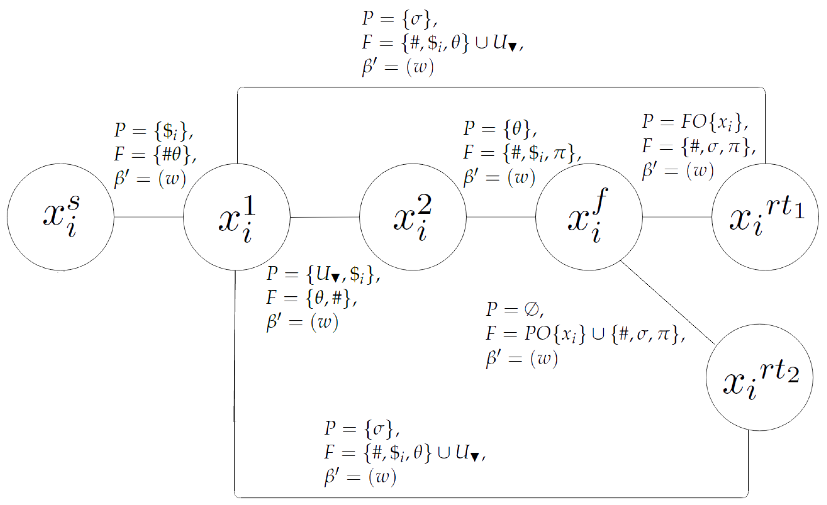
For each node $x_i\mid 1\le i\le n-1$ in $\Gamma$, we add a subnetwork (Figure 2).to ${\Gamma }^{\prime }$ according to the cases considered in the sequel.

Case 1. If $x_i$ is a splicing node with $\beta \left(x_i\right)=\left(w\right)$, the subnetwork is defined as follows:

• $x_i^s$
  $S=\left\{[(\epsilon ,\psi );(\#,{\$}_i)]\right\}\cup \left\{[(\epsilon ,{\$}_i);(\#,\theta )]\right\}$
  $A=\{\#{\$}_i,\#\theta \}$
• $x_i^1$
  $S=\left\{[(a,b);(u_{▼},v_{▼})]\right]\mid [(a,b);(u,v)]\in S_{x_i},\{a,b,u,v\}\in U^{*}\left\}\right\}$
  $A=\{{z^k}_{▼}(u,v){\$}_i\mid 1\le k\le card\left(A_{x_i}\right),z^k\in A_{x_i}\}$
• $x_i^2$
  $S=\left\{[(\epsilon ,{\$}_i);(\#,\theta )]\right\}\cup \left\{[(\epsilon ,\sigma );(\#,\theta )]\right\}\cup \left\{[(\epsilon ,\theta );(\#,\#)]\right\}$
  $A=\{\#\theta ,\#\#\}$
• $x_i^f$
  $S=\{[(a,v_{▼});(\#,v\pi )]\mid a\in U^{*}\}\cup \{[(av,\pi );(\#v_{▼},t)]\mid \{a,v\}\in U^{*},t\in \{U^{*}\cup \left\{\theta \right\}\}\}\cup$
  $\{[(u_{▼},b);(\pi u,\#)]\mid b\in U^{*}\cup \left\{\theta \right\}\}\cup \{[(\pi ,ub);(t,u_{▼}\#)]\mid \{u,t\}\in U^{*},b\in \{U^{*}\cup \left\{\theta \right\}\}\}$
  $A=\{\pi u\#,\#v\pi \theta \}$
• ${x_i}^{r{t}_1}$
  $S=\left\{\right[(\epsilon ,\theta );(\#,\sigma )\left]\right\}$
  $A=\{\#\sigma \}$
• ${x_i}^{r{t}_2}$
  $S=\left\{\right[(\epsilon ,\theta );(\#,\sigma )\left]\right\}$
  $A=\{\#\sigma \}$

The edges between them are:

$\{x_i^s,x_i^1\}$:	$P=\left\{{\$}_i\right\}$,	$F=\{\#\theta \}$,	${\beta }^{\prime }=\left(w\right)$,
$\{x_i^1,x_i^2\}$:	$P=\left\{{\$}_i\right\}\cup U_{▼}$,	$F=\{\theta ,\#\}$,	${\beta }^{\prime }=\left(w\right)$,
$\{x_i^2,x_i^f\}$:	$P=\left\{\theta \right\}$,	$F=\{\#,{\$}_i,\pi \}$,	${\beta }^{\prime }=\left(w\right)$,
$\{x_i^f,{x_i}^{r{t}_1}\}$:	$P=FO\left\{x_i\right\}$,	$F=\{\#,\sigma ,\pi \}$,	${\beta }^{\prime }=\left(w\right)$,
$\{x_i^f,{x_i}^{r{t}_2}\}$:	$P=\varnothing$,	$F=PO\left\{x_i\right\}\cup \{\#,\sigma ,\pi \}$,	${\beta }^{\prime }=\left(w\right)$,
$\{{x_i}^{r{t}_1},x_i^1\}$:	$P=\left\{\sigma \right\}$,	$F=\{\#,{\$}_i,\theta \}\cup U_{▼}$,	${\beta }^{\prime }=\left(w\right)$,
$\{{x_i}^{r{t}_2},x_i^1\}$:	$P=\left\{\sigma \right\}$,	$F=\{\#,{\$}_i,\theta \}\cup U_{▼}$,	${\beta }^{\prime }=\left(w\right)$,

Case 2. If $x_i$ is a splicing node with strong filters, we replace the node ${x_i}^{r{t}_2}$ with $p\ge 1$ nodes of the form ${x_i}^{r{t}_2^k}$, $1\le k\le p$, where $P{O}_{x_i}=\{Z_1,Z_2,\cdots ,Z_p\}$, $p\ge 1$. These new nodes are defined as follows:

$${x_i}^{r{t}_2^k}:S=\left\{[(\epsilon ,\theta );(\#,\sigma )]\right\},A=\{\#\sigma \},$$

and the edges between ${x_i}^{r{t}_2}$ and the nodes $x_i^f$ and $x_i^s$ are replaced with $2p$ edges of the form

$$\{x_i^f,{x_i}^{r{t}_2^k}\}:P=\varnothing ,F=\{Z_k,\#,\sigma ,\pi \}\cup U_{▼},{\beta }^{\prime }=\left(w\right),$$

$$\{{x_i}^{r{t}_2^k},x_i^1\}:P=\left\{\sigma \right\},F=\{\#,{\$}_i,\theta \}\cup U_{▼},{\beta }^{\prime }=\left(w\right)$$

In both cases, if $P{O}_{x_i}=\varnothing$, then the nodes ${x_i}^{r{t}_2}$ and ${x_i}^{r{t}_2^k}$ are removed. Analogously, if $F{O}_{x_i}=\varnothing$, then ${x_i}^{r{t}_1}$ is removed.

We now analyze a computation of ${\Gamma }^{\prime }$ on the input string $w=<z>$. In the input node $x_I$, the symbol $\psi$ is attached at the end of the string. Next, it enters $x_1^s$ and the simulation of a computation in $\Gamma$ starts. We assume that $w\psi$ lies in $x_1^s$ while the string w is found in $x_1$, the input node of $\Gamma$. Inductively, we may assume that a string w is found in some $x_i$, a node of $\Gamma$, as well as $w\psi$ in $x_i^s$ from ${\Gamma }^{\prime }$.

Let $x_i$ be a splicing node, where a rule $\left[\right(a,b\left)\right);(u,v)]$ is applied to w producing ${\alpha }_{1}av{\beta }_2$ and ${\beta }_{1}ub{\alpha }_2$, if $w={\alpha }_{1}ab{\alpha }_2$ or w otherwise. In ${\Gamma }^{\prime }$, the string $w\psi$ is processed as follows. First $w\psi$ becomes $w{\$}_i$ in $x_i^s$, then it can enter $x_i^1$ only. Here, it may become $w^{\prime }={\alpha }_{1}a{v}_{▼}{\beta }_2{\$}_i$ or $w^{\prime }={\beta }_1{u}_{▼}b{\alpha }_2{\$}_i$, if $w={\alpha }_{1}ab{\alpha }_2$, or it is left unchanged.

Further, a string of the form $w^{\prime }{\$}_i$ produced in this node can go back to $x_i^s$, where ${\$}_i$ is changed to $\theta$, sealing that string in the node. On the other hand, the strings can also enter $x_i^2$. In $x_i^2$, the symbols ${\$}_i$ and $\sigma$ are replaced by $\theta$, closing the route back to $x_i^1$. Note that the other produced strings $\#{\$}_i$, $\#\sigma$ and $\#\theta$ remain locked in the node.

Finally, the strings enter $x_i^f$ where each symbol $c\in u_{▼}$ or $c\in v_{▼}$, if present, is rewritten into the associated symbol c, replacing $u_{▼}$ with u and $v_{▼}$ with v. Thoroughly, the string $w={\alpha }_{1}a{v}_{▼}{\beta }_2\theta$ is split into the strings $w_1={\alpha }_{1}av\pi \theta$ and $w_2=\#v_{▼}{\beta }_2\theta$. Both strings cannot leave the node because of the characters $\pi$ and #. In the next splicing step, the only rule that can be applied to these strings is $\{[(av,\pi );(\#v_{▼},t)]$. At the same time, this rule can only be applied to these two new strings. The rule yields $w_1^{\prime }={\alpha }_{1}av{\beta }_2\theta$ and $w_2^{\prime }=\#v_{▼}\pi \theta$. The former contains the string generated by the original node $x_i$, $w_1={\alpha }_{1}av{\beta }_2$, completing the simulation of the splicing step. On the other hand, the latter cannot exit the node or be modified by any rule, so it remains locked for the rest of the computation. The logic is analogous for the other string generated by the splicing rule. Thus, in node $x_i^f$, we have obtained the strings ${\alpha }_{1}av{\beta }_2\theta$ and ${\beta }_{1}ub{\alpha }_2\theta$, if $w=\alpha ab{\alpha }_2$.

In conclusion, if $w\in U^{*}$ is a string in the nodes $x_i$ of $\Gamma$ and $w\psi$ in $x_i^s$ of ${\Gamma }^{\prime }$, then we can obtain $w^{\prime }\in U^{*}$ in one splicing step of $\Gamma$ if and only if we can obtain the associated string $w^{\prime }\theta$ in the node $x_i^f$ of ${\Gamma }^{\prime }$ in 4 splicing steps (or 8 computational steps). At this point, we note that $w^{\prime }$ can leave $x_i$ and enter $x_j$ in $\Gamma$ if and only if the string can leave $x_i^f$ and enter $x_j^s$ via the nodes $x_{i,j}^1$ and $x_{i,j}^2$. If it can leave $x_i$, but cannot enter $x_j$ in $\Gamma$, then it is trapped in $x_{i,j}^2$ in ${\Gamma }^{\prime }$. Furthermore, a string entering $x_j$ has the character $\psi$ replaced with ${\$}_j$, and consequently, it cannot return back to $x_{i,j}^2$. Finally, if the string cannot leave the node $x_i$, then it is sent by $x_i^f$ to ${x_i}^{r{t}_1}$ and ${x_i}^{r{t}_2}$ (in the case of weak filters) or to the nodes ${x_i}^{r{t}_1}$ and ${x_i}^{r{t}_2^k}$, for all $Z_k\in PO\left(x_i\right)$ (in the case of strong filters). In these nodes, the character $\theta$ is replaced with $\sigma$, and the resulting string is sent to $x_i^1$. If the string is not split in the following splicing step, it returns to the nodes ${x_i}^{r{t}_1}$ and ${x_i}^{r{t}_2}$ in the case of weak filters or to the nodes ${x_i}^{r{t}_1}$ and ${x_i}^{r{t}_2^k}$ in the case of strong filters, starting a ping-pong process between them, which continues until the string yields new ones by means of another splicing step in $x_i^1$. In this last case, the new strings can only enter $x_i^2$ because it contains characters $a_{▼}\in u_{▼}$ and the process described above is repeated.

We now analyze the computational steps required for simulating a computation in $\Gamma$. The input node $x_I$ and the node $x_1^s$ require 1 splicing step (or 2 computational steps) each. In the worst case, a splicing step in one of the nodes $\{x_i\mid 1\le i\le n-1\}$ can be simulated in ${\Gamma }^{\prime }$ in 7 splicing steps (or 14 computational steps) distributed in the following way:

• 2 steps in $x_i^1$.
• 2 steps in $x_i^2$.
• 4 steps in $x_i^f$.
• 2 steps in $x_{i,j}^1$.
• 2 steps in $x_{i,j}^2$.
• 2 steps in $x_j^s$.

Note that the simulation only requires 12 computational steps if $x_j^s\equiv x_n^s$ since the computation halts when a string enters $x_n^s$. We conclude that $L(\Gamma )=L\left({\Gamma }^{\prime }\right)$ and $Tim{e}_{{\Gamma }^{\prime }}\left(n\right)\in \mathcal{O}\left(Tim{e}_{\Gamma }\left(n\right)\right)$. □

The converse of the previous proposition holds.

Proposition 4. 

${\mathbf{Time}}_{NSPFC}\left(f\left(n\right)\right)\subseteq {\mathbf{Time}}_{NSP}\left(f\left(n\right)\right)$ for any function $f:IN\to IN$.

Proof. 

Let $\Gamma =(V,U,<,>,G,\mathcal{N},\beta ,x_1,x_n)$ be a NSPFC with $G=(X_G,E_G)$, $X_G$ having n nodes $x_1,x_2,\cdots ,x_n$; $x_1\equiv \underline{In}$ and $x_n\equiv \underline{Halt}$. We construct the NSP ${\Gamma }^{\prime }=(V^{\prime },U^{\prime },<,>,G^{\prime },{\mathcal{N}}^{\prime }$, ${\beta }^{\prime }$, $x_I,x_n^s)$; $x_I\equiv \underline{In}$ and $x_n^s\equiv \underline{Halt}$, where

$V^{\prime }=V$,	$U^{\prime }=U\cup U_{▼}\cup X\cup Y\cup \{\#,\psi \}$,
$X=\{X_i,X_i^{\prime }\mid 1\le i\le n\}$,	$Y=\{Y_i\mid 1\le i\le n-1\}$,
$U_{▼}=\{a_{▼}\mid a\in U\}$	$u_{▼}=a_{▼}^1{a}_{▼}^2\cdots a_{▼}^{\left|u\right|}\mid u=a^1{a}^2\cdots a^{\left|u\right|}\in U^{*}$,
$z_{▼}(u,v)={\beta }_1{u}_{▼}{v}_{▼}{\beta }_2\mid z={\beta }_{1}uvs.{\beta }_2\in U^{*}$

We now define the parameters of ${\Gamma }^{\prime }$. First, we add a main subnetwork composed by the input node $x_I$, the nodes $\{x_i^s\mid 1\le i\le n\}$, the nodes $\{x_i^1,x_i^2\mid 1\le i\le n-1\}$ and the nodes $\{x_{i,j}\mid 1\le i\ne j\le n,i\ne n,\mathrm{and}\{x_i,x_j\}\in E_G\}$.

• node $x_I$:
  $S=\left\{[(\epsilon ,>);(\#,>X_1)]\right\}$,
  $A=\{\#>X_1\}$
  – $PI=V$, $FI=X$, $PO=X$, $FO=\varnothing$,
  – ${\beta }^{\prime }=\left(w\right)$.
• nodes $x_i^s$, $1\le i\le n-1$:
  $S=\left\{[(a,b);(u_{▼},v_{▼})]\right]\mid [(a,b);(u,v)]\in S_{x_i},\{a,b,u,v\}\in U^{*}\}$,
  $A=\{{z^k}_{}(u,v)X_i\mid 1\le k\le card\left(A_{x_i}\right),z^k\in A_{x_i}\}$,
  – $PI=\{X_i,\psi \}$, $FI=X\setminus \left\{X_i\right\}\cup \{\#\}$, $PO=\{X_i,U_{▼}\}$, $FO=\varnothing$,
  – ${\beta }^{\prime }=\left(w\right)$.
• node $x_n^s$:
  $S=S\left(x_n\right)$,
  $A=A\left(x_n\right)$,
  – $PI=\{X_n,\psi \}$, $FI=X\setminus \left\{X_n\right\}\cup \{\#\}$, $PO=\{X_n,U_{▼}\}$, $FO=\varnothing$,
  – ${\beta }^{\prime }=\left(w\right)$.
• nodes $x_i^1$, $1\le i\le n-1$:
  $S=\left\{[(\epsilon ,X_i);(\#,X_i^{\prime })]\right\}\cup [(\epsilon ,\psi );(\#,X_i^{\prime })]]$,
  $A=\{\#X_i^{\prime }\}$,
  – $PI=\{X_i,U_{▼}\}$, $FI=\{\#\}$, $PO=\left\{X_i^{\prime }\right\}$, $FO=\varnothing$,
  – ${\beta }^{\prime }=\left(w\right)$.
• nodes $x_i^2$, $1\le i\le n-1$:
  $S=\{[(a,v_{▼});(\#,v\pi )]\mid a\in U^{*}\}\cup \{[(av,\pi );(\#v_{▼},t)]\mid \{a,v\}\in U^{*},t\in \{U^{*}\cup \{X_i,X_i^{\prime }\psi \}\}\}\cup$
  $\{[(u_{▼},b);(\pi u,\#)]\mid b\in U^{*}\cup \left\{\theta \right\}\}\cup \{[(\pi ,ub);(t,u_{▼}\#)]\mid \{u,t\}\in U^{*},b\in \{U^{*}\cup \{X_i,X_i^{\prime },\psi \}\}\}$,
  $A=\{\pi u\#,\#v\pi X_i^{\prime }\}$,
  – $PI=\left\{X_i^{\prime }\right\}$, $FI=\{\#\}$, $PO=\left\{X_i^{\prime }\right\}$, $FO=\{\pi ,\#\}$,
  – ${\beta }^{\prime }=\left(w\right)$.
• nodes $x_{i,j}$, $1\le i\ne j\le n,i\ne n,\{x_i,x_j\}\in E_G$:
  $S=\left\{[(\epsilon ,X_i^{\prime });(\#,X_j)]\right]\}$,
  $A=\{\#X_j\}$,
  – $PI=P_{\{x_i,x_j\}}$, $FI=F_{\{x_i,x_j\}}\cup \left\{X_j\right\}$, $PO=\left\{X_j\right\}$, $FO=\{\#\}$,
  – ${\beta }^{\prime }=\beta \left(\{x_i,x_j\}\right)$.

The edges between them are:

$$\left\{\{x_I,x_1^s\}\right\}\cup$$

$$\{\{x_i^s,x_i^1\}\mid 1\le i\le n-1\}\cup$$

$$\{\{x_i^1,x_i^2\}\mid 1\le i\le n-1\}\cup$$

$$\{\{x_i^2,x_{i,j}\}\mid 1\le i\ne j\le n,i\ne n,\mathrm{and}\{x_i,x_j\}\in E_G\}\}\cup$$

$$\{\{x_{i,j},x_j\}\mid 1\le i\ne j\le n,i\ne n,\mathrm{and}\{x_i,x_j\}\in E_G\}\},$$

Next, for each node $x_i\mid 1\le i\le n-1$ in $\Gamma$, we add a subnetwork to ${\Gamma }^{\prime }$ according to the cases considered in the sequel.

Case 1. Let $E_i$ be the number of nodes connected to the node $x_i^2$ of the form $x_{i,j}$, we add the corresponding nodes $\{x_{i,j}^{r{t}_1}\left(k\right),x_{i,j}^{r{t}_2}\left(k\right)\mid 1\le k\le E_i\}$ to the subnetwork. Note that $E_i$ is also equal to the number of edges between the node $x_i$ and the nodes $x_j\mid 1\le i\ne j\le n,i\ne n$ in the network $\Gamma$. If the edges $\{x_i,x_j\}\in \Gamma$ have $\beta =\left(w\right)$, the subnetwork is defined as follows:

• nodes $x_{i,j}^{r{t}_1}\left(k\right)$, $1\le k\le E_i,1\le i\ne j\le n,i\ne n,\{x_i,x_j\}\in E_G$:
  $S=\left\{\begin{array}{c}\left\{[(\epsilon ,X_i^{\prime });(\#,Y_2)]\right\},\mathrm{if}k=1\wedge E_i>1\hfill \\ \left\{[(\epsilon ,Y_k);(\#,Y_{k+1})]\right\},\mathrm{if}2\le k\le E_i-1\hfill \\ \left\{[(\epsilon ,Y_{E_i});(\#,\psi )]\right\},\mathrm{if}k=E_i\wedge E_i>1\hfill \\ \left\{[(\epsilon ,X_i^{\prime });(\#,\psi )]\right\},\mathrm{if}{E}_i=1\hfill \end{array}\right.$,
  $A=\left\{\begin{array}{c}\{\#Y_{k+1}\},\mathrm{if}1\le k\le E_i-1\hfill \\ \{\#\psi \},\mathrm{if}k=E_i\hfill \end{array}\right.$,
  – $PI=F_{\{x_i,x_j\}}$, $FI=\{\#,\psi \}\cup \{Y\setminus Y_k\}$, $PO=\{\psi ,Y_{k+1}\}$, $FO=\{\#\}$,
  – ${\beta }^{\prime }=\left(w\right)$.
• nodes $x_{i,j}^{r{t}_2}\left(k\right)$, $1\le k\le E_i,1\le i\ne j\le n,i\ne n,\{x_i,x_j\}\in E_G$:
  $S=\left\{\begin{array}{c}\left\{[(\epsilon ,X_i^{\prime });(\#,Y_2)]\right\},\mathrm{if}k=1\wedge E_i>1\hfill \\ \left\{[(\epsilon ,Y_k);(\#,Y_{k+1})]\right\},\mathrm{if}2\le k\le E_i-1\hfill \\ \left\{[(\epsilon ,Y_{E_i});(\#,\psi )]\right\},\mathrm{if}k=E_i\wedge E_i>1\hfill \\ \left\{[(\epsilon ,X_i^{\prime });(\#,\psi )]\right\},\mathrm{if}{E}_i=1\hfill \end{array}\right.$,
  $A=\left\{\begin{array}{c}\{\#Y_{k+1}\},\mathrm{if}1\le k\le E_i-1\hfill \\ \{\#\psi \},\mathrm{if}k=E_i\hfill \end{array}\right.$,
  – $PI=\varnothing$, $FI=P_{\{x_i,x_j\}}\cup \{\#,\psi \}\cup \{Y\setminus Y_k\}$, $PO=\{\psi ,Y_{k+1}\}$, $FO=\{\#\}$,
  – ${\beta }^{\prime }=\left(w\right)$.

The edges between them are:

$$\{\{x_i^2,x_{i,j}^{r{t}_1}\left(1\right)\},\{x_i^2,x_{i,j}^{r{t}_2}\left(1\right)\}\}\cup$$

$$\{\{x_{i,j}^{r{t}_1}\left(k\right),x_{i,j}^{r{t}_1}(k+1)\},\{x_{i,j}^{r{t}_1}\left(k\right),x_{i,j}^{r{t}_2}(k+1)\}\mid 1\le k\le E_i-1\}\cup$$

$$\{\{x_{i,j}^{r{t}_2}\left(k\right),x_{i,j}^{r{t}_1}(k+1)\},\{x_{i,j}^{r{t}_2}\left(k\right),x_{i,j}^{r{t}_2}(k+1)\}\mid 1\le k\le E_i-1\}\cup$$

$$\{\{x_{i,j}^{r{t}_1}\left(E_i\right),x_i^s\},\{x_{i,j}^{r{t}_2}\left(E_i\right),x_i^s\}\},$$

Case 2. If the k edge $\{x_i,x_j\}$ has $\beta =\left(s\right)$, we replace each of the nodes $x_{i,j}^{r{t}_2}\left(k\right)$ for $p\ge 1$ nodes of the form $x_{i,j}^{r{t}_2^t}\left(k\right)$, $1\le t\le p$, where $P_{\{x_i,x_j\}}=\{Z_1,Z_2,\cdots ,Z_p\}$, $p\ge 1$. The parameters S, A and $\beta$ of these new nodes remain the same, while the input and output filters are defined as follows:

$$x_{i,j}^{r{t}_2^t}\left(k\right):PI=\varnothing ,FI=\{Z_t,\#,\psi \}\cup \{Y\setminus Y_k\},PO=\{\psi ,Y_{k+1}\},FO=\{\#\}$$

and the edges involving $x_{i,j}^{r{t}_2}\left(k\right)$ are replaced with p edges involving each of the nodes $x_{i,j}^{r{t}_2^t}\left(k\right)$.

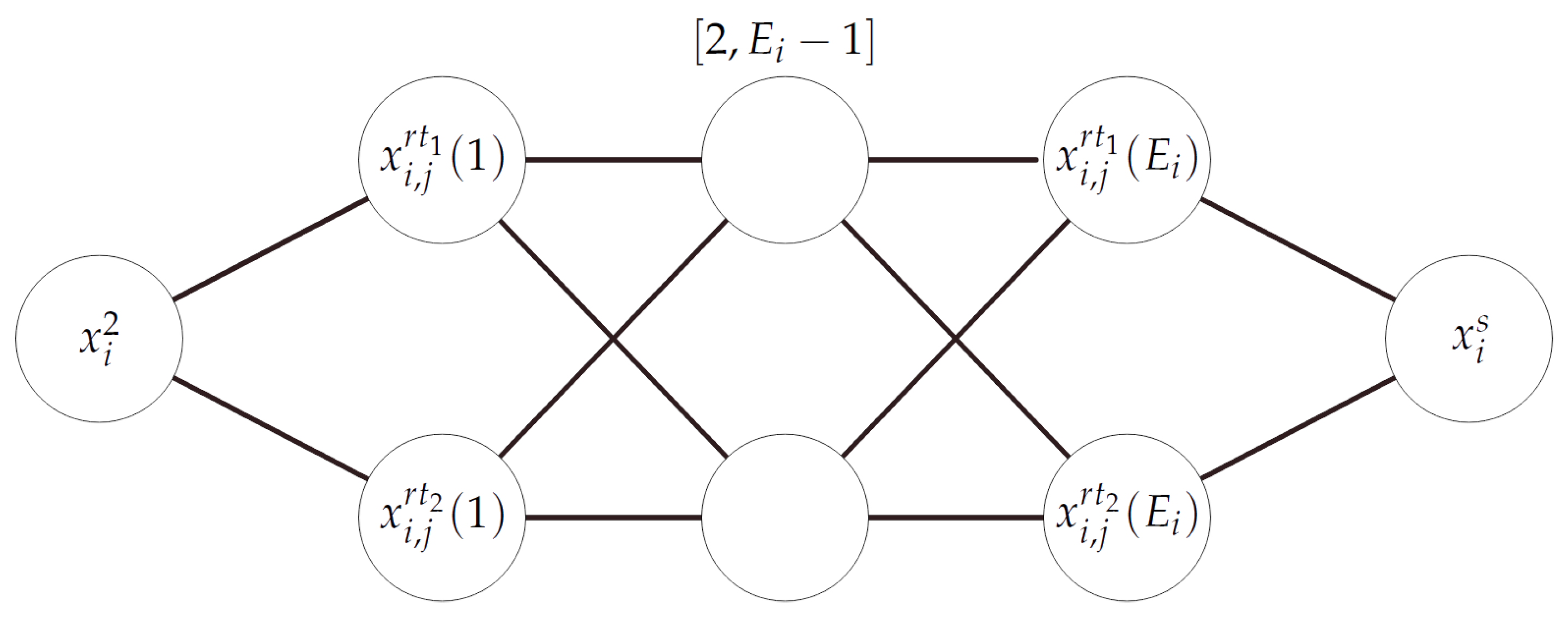
In both cases, if the k edge has $P_{\{x_i,x_j\}}=\varnothing$, then the nodes $x_{i,j}^{r{t}_2}\left(k\right)$ and $x_{i,j}^{r{t}_2^t}\left(k\right)$ are removed. Analogously, if $F_{\{x_i,x_j\}}=\varnothing$, then $x_{i,j}^{r{t}_1}\left(k\right)$ is removed. Furthermore, if $P_{\{x_i,x_j\}}=\varnothing$ and $F_{\{x_i,x_j\}}=\varnothing$, the whole subnetwork given in Figure 3 is removed because a string is always able to leave the node $x_i\in \Gamma$ through the edge k.

Let us assume the string $w=<z>$ to be the input string in $\Gamma$. In the input node $x_I$ of ${\Gamma }^{\prime }$, the symbol $X_1$ is attached to the string and then sent to the node $x_1^s$. Thus, the node $x_1\in \Gamma$ contains the string $w=<z>$ while $w=<z>X_1$ lies in the analogous node $x_1^s\in {\Gamma }^{\prime }$. In a more general setting, we assume that a string $y^{\prime }=y{X}_i$, $y\in U^{*}$, enters $x_i^s\in {\Gamma }^{\prime }$ at a given step of the computation of ${\Gamma }^{\prime }$ on w if and only if the string y enters $x_i\in \Gamma$ at a given step of the computation of $\Gamma$ on w.

Let y be transformed into $z_1={\alpha }_{1}avs.{\beta }_2$ and $z_2={\beta }_{1}ub{\alpha }_2$ in node $x_i$ and $z_1$ and/or $z_2$ can pass the filter on the edge between $x_i$ and $x_j$. In ${\Gamma }^{\prime }$, the string $y^{\prime }=y{X}_i$ is transformed into $z_1^{\prime }={\alpha }_{1}a{v}_{▼}{\beta }_2{X}_i$ and $z_2^{\prime }={\beta }_1{u}_{▼}b{\alpha }_2{X}_i$ in the node $x_i^s$. If the string is of the form $y^{\prime }=y\psi$, it is transformed into $z_1^{\prime }={\alpha }_{1}a{v}_{▼}{\beta }_2{X}_i$ and $z_2^{\prime }={\beta }_1{u}_{▼}b{\alpha }_2\psi$. The strings enter $x_i^1$ where the characters $X_i$ and $\psi$ are replaced with $X_i^{\prime }$. Thus, we get the same strings with either $X_i$ or $\psi$. Then, it continues into $x_i^2$, where the symbols in $u_{▼}$ and $v_{▼}$, if present, are replaced with the original counterpart u and v. In detail, the string $z_1^{\prime }$ is split into the strings $z_1\left(1\right)={\alpha }_{1}av\pi X_i^{\prime }$ and $z_1\left(2\right)=\#v_{▼}{\beta }_2{X}_i^{\prime }$. Both strings cannot leave the node because of the characters $\pi$ and #. In the next splicing step, the rule $\{[(av,\pi );(\#v_{▼},t)]$ is applied to the two strings, yielding $z_1{\left(1\right)}^{\prime }={\alpha }_{1}avs.{\beta }_2{X}_i^{\prime }$ and $z_2{\left(2\right)}^{\prime }=\#v_{▼}\pi X_i^{\prime }$. The former constitutes the string $z=z_1{X}_i^{\prime }$ where $z_1$ is the string yielded by $x_i\in \Gamma$, completing the simulation of the application of a splicing rule of $\Gamma$. On the other hand, the latter cannot exit the node or be modified by any rule, so it remains locked for the rest of the computation. The logic is analogous for the other string generated by the splicing rule. The new string $z=z_1{X}_i^{\prime }$ is sent to the nodes $x_{i,j}$ associated to the edges $\{x_i,x_j\}$ in the original network. Since the input filters of these nodes are identical to the edge filters in $\Gamma$, the string $z_1{X}_i^{\prime }$ can enter a node $x_{i,j}\in {\Gamma }^{\prime }$ if and only if the string $z_1$ can pass the filter between $x_i$ and $x_j$ in $\Gamma$. Note that the converse is also true. Subsequently, the symbol $X_i^{\prime }$ is replaced with $X_j$ and the new string is sent to $x_j^s\in {\Gamma }^{\prime }$ where a similar procedure starts. Alternatively, if the string y is not split in $x_i\in \Gamma$, the same event happens in $x_i^s\in {\Gamma }^{\prime }$. If the string is of the form $y^{\prime }=y\psi$, it remains locked in that node until a splicing rule can be applied on it while a string of the form $y^{\prime }=y{X}_i$ still enters the node $x_i^1$ because of the symbol $X_i$ and the same computational process described above starts.

On the other hand, a copy of the string $z{X}_i^{\prime }$ is also sent to the subnetwork illustrated in Figure 3, where the case of a string not passing the filters of any edge between the node $x_i$ and the connected nodes in the original network $\Gamma$ is handled. We distinguish here between the cases of strong and weak filters. For each edge k with $\beta =\left(w\right)$, $1\le k\le E_i$, the node $x_{i,j}^{r{t}_1}\left(k\right)$ checks if the string cannot enter the corresponding node $x_{i,j}\left(k\right)$ because of containing forbidden symbols, while the node $x_{i,j}^{r{t}_2}\left(k\right)$ verifies if the string contains the characters required by the $PI$ filter of the node $x_{i,j}\left(k\right)$. Thoroughly, the string exits $x_i^2$ and enters the first pair of nodes $x_{i,j}^{r{t}_1}\left(1\right)$ and $x_{i,j}^{r{t}_2}\left(1\right)$ granted that the associated string z could not pass the filters of the first edge in the network $\Gamma$. In that node, $X_i^{\prime }$ is replaced with $Y_2$ ensuring that the new string could only enter the next pair of nodes $x_{i,j}^{r{t}_1}\left(2\right)$ and $x_{i,j}^{r{t}_2}\left(2\right)$ associated to the second edge. Subsequently, $Y_k\mid 2\le k\le E_i-1$ is replaced by the next character $Y_{k+1}$ in the remaining pair of nodes $x_{i,j}^{r{t}_1}\left(k\right)$ and $x_{i,j}^{r{t}_2}\left(k\right)$, forcing the string to continue through them in sequence. If the string can enter one of the connected nodes through an edge in $\Gamma$, it will be lost at some point of this subnetwork as it will be refused by the input filters of the nodes corresponding to that edge. Otherwise, it will reach the last pair of nodes where the symbol $Y_{E_i}$ will be changed to $\psi$, yielding a string of the form $z\psi$ which will be returned to $x_i^s$. Because of the character $\psi$, this string cannot leave the node $x_i^s$ ensuring it remains there until it can be used in a new splicing step. Thus, the following computational step in $\Gamma$ was simulated in ${\Gamma }^{\prime }$: z could not leave the node $x_i$ and it remained in that node for new splicing steps. In the case of an edge k with strong filters, the computation follows the same procedure described above with the difference that the node $x_{i,j}^{r{t}_2}\left(k\right)$ is replaced with $p\ge 1$ nodes of the form $x_{i,j}^{r{t}_2^t}\left(k\right)$, $1\le t\le p$, where $P_{\{x_i,x_j\}}=\{Z_1,Z_2,\cdots ,Z_p\}$, $p\ge 1$. A node $x_{i,j}^{r{t}_2^t}\left(k\right)$ refuses any string z containing the character $Z_t$. Thus, the string can only continue through this network by means of a node $x_{i,j}^{r{t}_2^t}\left(k\right)$ for some $1\le t\le p$ if it only contains a proper subset of $P_{\{x_i,x_j\}}$.

We analyze now the case where a string $z{X}_i^{\prime }$ enters $x_{i,n}$ from a node $x_i^2$, for some $1\le i\le n-1$. In that node, $X_i^{\prime }$ is replaced with $X_n$ and the resulting string enters $x_n^s$, ending the computation. Note that by the considerations above, a string enters $x_{i,n}$ if and only if a string from $x_i$ was able to pass the filter on the edge between $x_i$ and $x_n$ in $\Gamma$.

We now analyze the computational steps required for simulating a computation in $\Gamma$. The input node $x_I$ requires 1 splicing step (or 2 computational steps). In the worst case, a splicing step in one of the nodes $\{x_i\mid 1\le i\le n-1\}$ can be simulated in the associated subnetwork in $4+E_i$ splicing steps (or $8+2E_i$ computational steps) distributed in the following way:

• 2 steps in $x_i^s$.
• 2 steps in $x_i^1$.
• 4 steps in $x_i^2$.
• 2 steps in $x_{i,j}$ if the string z yielded by the splicing step in the node $x_i\in \Gamma$ could pass any of the edge filters between $x_i$ and $x_j$ in $\Gamma$; $1\le i\ne j\le n,i\ne n$.
• $2E_i$ steps if z could not pass any of the edge filters in $\Gamma$.

Since $E_i$ is bounded by $n-1$, where n is the number of nodes in $\Gamma$, a NSPFC can be simulated by NSP in $\mathcal{O}\left(n\right)$ time. As a result of this analysis, we conclude that $L(\Gamma )=L\left({\Gamma }^{\prime }\right)$ and $Tim{e}_{{\Gamma }^{\prime }}\left(n\right)\in \mathcal{O}\left(Tim{e}_{\Gamma }\left(n\right)\right)$. □

5. Direct Simulations between NUSPs and NSPFCs

Proposition 5. 

${\mathbf{Time}}_{NUSP}\left(f\left(n\right)\right)\subseteq {\mathbf{Time}}_{NSPFC}\left(f\left(n\right)\right)$ for any function $f:IN\to IN$.

Proof. 

This proposition can be proved through a NSPFC simulation of NUSP identical to the proposed simulation for NSP in the previous section, with the only difference being the replacement of the filters $PI,PO$ with P and $FI,FO$ with F in the specifications.

Therefore, the input node $x_I$ and the node $x_1^s$ require 1 splicing step (or 2 computational steps) each. In the worst case, a splicing step in one of the nodes $\{x_i\mid 1\le i\le n-1\}$ can be simulated in ${\Gamma }^{\prime }$ in 7 splicing steps (or 14 computational steps) distributed in the following way:

• 2 steps in $x_i^1$.
• 2 steps in $x_i^2$.
• 4 steps in $x_i^f$.
• 2 steps in $x_{i,j}^1$.
• 2 steps in $x_{i,j}^2$.
• 2 steps in $x_j^s$.

Similarly, we conclude that $L(\Gamma )=L\left({\Gamma }^{\prime }\right)$ and $Tim{e}_{{\Gamma }^{\prime }}\left(n\right)\in \mathcal{O}\left(Tim{e}_{\Gamma }\left(n\right)\right)$. □

The converse of the previous proposition holds.

Proposition 6. 

${\mathbf{Time}}_{NSPFC}\left(f\left(n\right)\right)\subseteq {\mathbf{Time}}_{NUSP}\left(f\left(n\right)\right)$ for any function $f:IN\to IN$.

Proof. 

Let $\Gamma =(V,U,<,>,G,\mathcal{R},\mathcal{N},\alpha ,x_1,x_n)$ be a NSPFC with $G=(X_G,E_G)$, $X_G$ having n nodes $x_1,x_2,\cdots ,x_n$; $x_1\equiv \underline{In}$ and $x_n\equiv \underline{Halt}$. We construct the NUSP ${\Gamma }^{\prime }=(V,U^{\prime },<,>.G^{\prime },{\mathcal{N}}^{\prime }$, ${\alpha }_1^{\prime }$, $x_I,x_n^s)$; $x_I\equiv \underline{In}$ and $x_n^s\equiv \underline{Halt}$, where

$V^{\prime }=V$,	$U^{\prime }=U\cup U_{▼}\cup X\cup Y\cup \{\#,\psi \}$,
$X=\{X_i,X_i^{\prime }\mid 1\le i\le n\}$,	$Y=\{Y_i\mid 1\le i\le n-1\}$,
$U_{▼}=\{a_{▼}\mid a\in U\}$	$u_{▼}=a_{▼}^1{a}_{▼}^2\cdots a_{▼}^{\left|u\right|}\mid u=a^1{a}^2\cdots a^{\left|u\right|}\in U^{*}$,
$z_{▼}(u,v)={\beta }_1{u}_{▼}{v}_{▼}{\beta }_2\mid z={\beta }_{1}uvs.{\beta }_2\in U^{*}$

We now define the parameters of ${\Gamma }^{\prime }$. First, we add a main subnetwork composed by the input node $x_I$, the nodes $\{x_i\mid 1\le i\le n\}$, the nodes $\{x_i^1,x_i^2\mid 1\le i\le n-1\}$ and the nodes $\{x_{i,j}\mid 1\le i\ne j\le n,i\ne n,\mathrm{and}\{x_i,x_j\}\in E_G\}$.

• node $x_I$:
  $S=\left\{[(\epsilon ,>);(\#,>X_1^{\prime })]\right\}$,
  $A=\{\#>X_1^{\prime }\}$
  – $P=V$, $F=\{\#,X_1\}$,
  – ${\beta }^{\prime }=\left(w\right)$.
• node $x_I^1$:
  $S=\left\{[(\epsilon ,X_1^{\prime });(\#,X_1)]\right\}\cup \left\{[(\epsilon ,X_1);(\#,\#)]\right\}$,
  $A=\{\#X_1,\#\#\}$
  – $P=\{X_1,X_1^{\prime }\}$, $F=\{\#\}$,
  – ${\beta }^{\prime }=\left(w\right)$.
• nodes $x_i^s$, $1\le i\le n-1$:
  $S=\left\{[(a,b);(u_{▼},v_{▼})]\right]\mid [(a,b);(u,v)]\in S_{x_i},\{a,b,u,v\}\in U^{*}\}$,
  $A=\{{z^k}_{▼}(u,v)X_i\mid 1\le k\le card\left(A_{x_i}\right),z^k\in A_{x_i}\}$,
  – $P=\{X_i,\psi ,U_{▼}\}$, $F=X\setminus \left\{X_i\right\}\cup \{\#\}$,
  – ${\beta }^{\prime }=\left(w\right)$.
• nodes $x_n^s$:
  $S=S\left(x_n\right)$,
  $A=A\left(x_n\right)$,
  – $P=\{X_n,\psi ,U_{▼}\}$, $F=X\setminus \left\{X_n\right\}\cup \{\#\}$,
  – ${\beta }^{\prime }=\left(w\right)$.
• nodes $x_i^1$, $1\le i\le n-1$:
  $S=\left\{[(\epsilon ,X_i);(\#,X_i^{\prime })]\right\}\cup [(\epsilon ,\psi );(\#,X_i^{\prime })]]\cup [(\epsilon ,X_i^{\prime });(\#,\#)]]$,
  $A=\{\#X_i^{\prime },\#\#\}$,
  – $P=\{X_i,X_i^{\prime },U_{▼}\}$, $F=\{\#\}$,
  – ${\beta }^{\prime }=\left(w\right)$.
• nodes $x_i^2$, $1\le i\le n-1$:
  $S=\{[(a,v_{▼});(\#,v\pi )]\mid a\in U^{*}\}\cup \{[(av,\pi );(\#v_{▼},t)]\mid \{a,v\}\in U^{*},t\in \{U^{*}\cup \{X_i,X_i^{\prime }\psi \}\}\}\cup$
  $\{[(u_{▼},b);(\pi u,\#)]\mid b\in U^{*}\cup \left\{\theta \right\}\}\cup \{[(\pi ,ub);(t,u_{▼}\#)]\mid \{u,t\}\in U^{*},b\in \{U^{*}\cup \{X_i,X_i^{\prime },\psi \}\}\}$,
  $A=\{\pi u\#,\#v\pi X_i^{\prime }\}$,
  – $P=\left\{X_i^{\prime }\right\}$, $F=\{\pi ,\#\}$,
  – ${\beta }^{\prime }=\left(w\right)$.
• nodes $x_{i,j}$, $1\le i\ne j\le n,i\ne n,\{x_i,x_j\}\in E_G$:
  $S=\left\{[(\epsilon ,X_i^{\prime });(\#,X_j)]\right]\}\cup \left\{[(\epsilon ,X_j);(\#,\#)]\right]\}$,
  $A=\{\#X_j,\#\#\}$,
  – $P=P_{\{x_i,x_j\}}$, $F=F_{\{x_i,x_j\}}$,
  – ${\beta }^{\prime }=\beta \left(\{x_i,x_j\}\right)$.

The edges between them are:

$$\left\{\{x_I,x_I^1\}\right\}\cup$$

$$\left\{\{x_I^1,x_1^s\}\right\}\cup$$

$$\{\{x_i^s,x_i^1\}\mid 1\le i\le n-1\}\cup$$

$$\{\{x_i^1,x_i^2\}\mid 1\le i\le n-1\}\cup$$

$$\{\{x_i^2,x_{i,j}\}\mid 1\le i\ne j\le n,i\ne n,\mathrm{and}\{x_i,x_j\}\in E_G\}\}\cup$$

$$\{\{x_{i,j},x_j^s\}\mid 1\le i\ne j\le n,i\ne n,\mathrm{and}\{x_i,x_j\}\in E_G\}\}.$$

Next, for each node $x_i\mid 1\le i\le n-1$ in $\Gamma$, we add a subnetwork to ${\Gamma }^{\prime }$ according to the cases considered in the sequel.

Case 1. Let $E_i$ be the number of nodes connected to the node $x_i^2$ of the form $x_{i,j}$, we add the corresponding nodes $\{x_{i,j}^{r{t}_1}\left(k\right),x_{i,j}^{r{t}_2}\left(k\right)\mid 1\le k\le E_i\}$ to the subnetwork. Note that $E_i$ is also equal to the number of edges between the node $x_i$ and the nodes $x_j\mid 1\le i\ne j\le n,i\ne n$ in the network $\Gamma$. If the edges $\{x_i,x_j\}\in \Gamma$ have $\beta =\left(w\right)$, the subnetwork is defined as follows:

• nodes $x_{i,j}^{r{t}_1}\left(k\right)$, $1\le k\le E_i,1\le i\ne j\le n,i\ne n,\{x_i,x_j\}\in E_G$:
  $S=\left\{\begin{array}{c}\left\{[(\epsilon ,X_i^{\prime });(\#,Y_2)]\right\}\cup \left\{[(\epsilon ,\psi );(\#,\#)]\right\},\mathrm{if}k=1\wedge E_i>1\hfill \\ \left\{[(\epsilon ,Y_k);(\#,Y_{k+1})]\right\}\cup \left\{[(\epsilon ,\psi );(\#,\#)]\right\},\mathrm{if}2\le k\le E_i-1\hfill \\ \left\{[(\epsilon ,Y_{E_i});(\#,\psi )]\right\},\mathrm{if}k=E_i\wedge E_i>1\hfill \\ \left\{[(\epsilon ,X_i^{\prime });(\#,\psi )]\right\},\mathrm{if}{E}_i=1\hfill \end{array}\right.$
  $A=\left\{\begin{array}{c}\{\#Y_{k+1},\#\#\},\mathrm{if}1\le k\le E_i-1\hfill \\ \{\#\psi \},\mathrm{if}k=E_i\hfill \end{array}\right.$,
  – $P=F_{\{x_i,x_j\}}$, $F=\{\#,X_i\}\cup \{Y\setminus \{Y_k,Y_{k+1}\}\}\cup \left\{U_{▼}\right\}$,
  – ${\beta }^{\prime }=\left(w\right)$.
• nodes $x_{i,j}^{r{t}_2}\left(k\right)$, $1\le k\le E_i,1\le i\ne j\le n,i\ne n,\{x_i,x_j\}\in E_G$:
  $S=\left\{\begin{array}{c}\left\{[(\epsilon ,X_i^{\prime });(\#,Y_2)]\right\}\cup \left\{[(\epsilon ,\psi );(\#,\#)]\right\},\mathrm{if}k=1\wedge E_i>1\hfill \\ \left\{[(\epsilon ,Y_k);(\#,Y_{k+1})]\right\}\cup \left\{[(\epsilon ,\psi );(\#,\#)]\right\},\mathrm{if}2\le k\le E_i-1\hfill \\ \left\{[(\epsilon ,Y_{E_i});(\#,\psi )]\right\},\mathrm{if}k=E_i\wedge E_i>1\hfill \\ \left\{[(\epsilon ,X_i^{\prime });(\#,\psi )]\right\},\mathrm{if}{E}_i=1\hfill \end{array}\right.$
  $A=\left\{\begin{array}{c}\{\#Y_{k+1},\#\#\},\mathrm{if}1\le k\le E_i-1\hfill \\ \{\#\psi \},\mathrm{if}k=E_i\hfill \end{array}\right.$,
  – $P=\varnothing$, $F=P_{\{x_i,x_j\}}\cup \{\#,X_i\}\cup \{Y\setminus \{Y_k,Y_{k+1}\}\}\cup \left\{U_{▼}\right\}$,
  – ${\beta }^{\prime }=\left(w\right)$.

The edges between them are:

$$\{\{x_i^2,x_{i,j}^{r{t}_1}\left(1\right)\},\{x_i^2,x_{i,j}^{r{t}_2}\left(1\right)\}\}\cup$$

$$\{\{x_{i,j}^{r{t}_1}\left(k\right),x_{i,j}^{r{t}_1}(k+1)\},\{x_{i,j}^{r{t}_1}\left(k\right),x_{i,j}^{r{t}_2}(k+1)\}\mid 1\le k\le E_i-1\}\cup$$

$$\{\{x_{i,j}^{r{t}_2}\left(k\right),x_{i,j}^{r{t}_1}(k+1)\},\{x_{i,j}^{r{t}_2}\left(k\right),x_{i,j}^{r{t}_2}(k+1)\}\mid 1\le k\le E_i-1\}\cup$$

$$\{\{x_{i,j}^{r{t}_1}\left(E_i\right),x_i^s\},\{x_{i,j}^{r{t}_2}\left(E_i\right),x_i^s\}\},$$

Case 2. If the k edge $\{x_i,x_j\}$ has $\beta =\left(s\right)$, we replace each of the nodes $x_{i,j}^{r{t}_2}\left(k\right)$ for $p\ge 1$ nodes of the form $x_{i,j}^{r{t}_2^t}\left(k\right)$, $1\le t\le p$, where $P_{\{x_i,x_j\}}=\{Z_1,Z_2,\cdots ,Z_p\}$, $p\ge 1$.The parameters S, A and $\beta$ of these new nodes remain the same, while the input and output filters are defined as follows:

$$x_{i,j}^{r{t}_2^t}\left(k\right):P=\varnothing ,F=\{Z_t,\#,X_i\}\cup \{Y\setminus \{Y_k,Y_{k+1}\}\}\cup \left\{U_{▼}\right\}$$

and the edges involving $x_{i,j}^{r{t}_2}\left(k\right)$ are replaced with p edges involving each of the nodes $x_{i,j}^{r{t}_2^t}\left(k\right)$.

In both cases, if the k edge has $P_{\{x_i,x_j\}}=\varnothing$, then the nodes $x_{i,j}^{r{t}_2}\left(k\right)$ and $x_{i,j}^{r{t}_2^t}\left(k\right)$ are removed. Analogously, if $F_{\{x_i,x_j\}}=\varnothing$, then $x_{i,j}^{r{t}_1}\left(k\right)$ is removed. Furthermore, if $P_{\{x_i,x_j\}}=\varnothing$ and $F_{\{x_i,x_j\}}=\varnothing$, the whole subnetwork given in in Figure 3 is removed because a string is always able to leave the node $x_i\in \Gamma$ through the edge k.

Let us assume the string $w=<z>$ to be the input string in $\Gamma$. In the input node $x_I$ of ${\Gamma }^{\prime }$, the symbol $X_1^{\prime }$ is attached to the string and then sent to the node $x_I^1$, where it is replaced with $X_1$. Then, the new string is sent to $x_1^s$ and the simulation process starts. Thus, the node $x_1\in \Gamma$ contains the string $w=<z>$ while $w=<z>X_i$ lies in the analogous node $x_1^s\in {\Gamma }^{\prime }$. In a more general setting, we assume that a string $y^{\prime }=y{X}_i$, $y\in U^{*}$, enters $x_i^s\in {\Gamma }^{\prime }$ at a given step of the computation of ${\Gamma }^{\prime }$ on w if and only if the string y enters $x_i\in \Gamma$ at a given step of the computation of $\Gamma$ on w. Note that any string entering $x_I^1$ from $x_1^s$ will have the character $X_1$ replaced with #, which will result in that string being locked in that node. Therefore, the two nodes $x_I$ and $x_I^1$ do not interfere with the computation anymore.

Let y be transformed into $z_1={\alpha }_{1}avs.{\beta }_2$ and $z_2={\beta }_{1}ub{\alpha }_2$ in node $x_i$ and $z_1$ and/or $z_2$ can pass the filter on the edge between $x_i$ and $x_j$. In ${\Gamma }^{\prime }$, the string $y^{\prime }=yc$, with $c\in \{X_i,\psi \}$, is transformed into $z_1^{\prime }={\alpha }_{1}a{v}_{▼}{\beta }_2{X}_i$ and $z_2^{\prime }={\beta }_1{u}_{▼}b{\alpha }_{2}c$. The strings enter $x_i^1$, where the characters $X_i$ and $\psi$ are replaced with $X_i^{\prime }$. Thus, we get the same strings with any $c\in \{X_i,\psi \}$. Then, it continues into $x_i^2$, where the symbols in $u_{▼}$ and $v_{▼}$, if present, are replaced with the original counterpart u and v. In detail, the string $z_1^{\prime }$ is split into the strings $z_1\left(1\right)={\alpha }_{1}av\pi X_i^{\prime }$ and $z_1\left(2\right)=\#v_{▼}{\beta }_2{X}_i^{\prime }$. Both strings cannot leave the node because of the characters $\pi$ and #. In the next splicing step, the rule $\{[(av,\pi );(\#v_{▼},t)]$ is applied to the two strings, yielding $z_1{\left(1\right)}^{\prime }={\alpha }_{1}avs.{\beta }_2{X}_i^{\prime }$ and $z_2{\left(2\right)}^{\prime }=\#v_{▼}\pi X_i^{\prime }$. The former constitutes the string $z=z_1{X}_i^{\prime }$ where $z_1$ is the string yielded by $x_i\in \Gamma$, completing the simulation of the splicing step. On the other hand, the latter cannot exit the node or be modified by any rule, so it remains locked for the rest of the computation. The logic is analogous for the other string generated by the splicing rule. The new string $z=z_1{X}_i^{\prime }$ is sent to the nodes $x_{i,j}$ associated to the edges $\{x_i,x_j\}$ in the original network. Since the filters of these nodes are identical to the edge filters in $\Gamma$, the string $z_1{X}_i^{\prime }$ can enter a node $x_{i,j}\in {\Gamma }^{\prime }$ if and only if the string $z_1$ can pass the filter between $x_i$ and $x_j$ in $\Gamma$. Note that the converse is also true. Subsequently, the symbol $X_i^{\prime }$ is replaced with $X_j$ and the new string is sent to $x_j^s\in {\Gamma }^{\prime }$ where a similar procedure starts. Note that if the string returns to the previous node in this sequence, it is ultimately blocked or lost. In $x_i^1$, the strings entering from $x_i^2$ are split into two strings containing the forbidden symbol # and consequently they remain locked in that node. The same situation happens if a string enters $x_i^2$ from a node $x_{i,j}$. On the other hand, if a string enters a node $x_{i,j}$ from $x_j^s$ for a given j, the string is split into two strings containing the symbol #. In the next communication step, these two strings are ejected from the network because they are not accepted by any node connected to $x_{i,j}$. Alternatively, if the string y remains unchanged in $x_i\in \Gamma$, the same event happens in $x_i^s\in {\Gamma }^{\prime }$. If the string is of the form $y^{\prime }=y\psi$, it starts a ping-pong process with the nodes $x_{i,j}^{r{t}_1}$ and $x_{i,j}^{r{t}_2}$ (or the nodes $x_{i,j}^{r{t}_2^t}\left(k\right)$ if the edge $\{x_i,x_j\}\in \Gamma$ has strong filters) until a splicing rule can be applied on it. On the other hand, if the string is of the form $y^{\prime }=y{X}_i$, it still enters the node $x_i^1$ because of the symbol $X_i$, starting the same computational process described above.

On the other hand, a copy of the string $z{X}_i^{\prime }$ is also sent to the subnetwork illustrated in Figure 3, where the case of a string not passing the filters of any edge between the node $x_i$ and the connected nodes in the original network $\Gamma$ is handled. We distinguish here between the cases of strong and weak filters. For each edge k with $\beta =\left(w\right)$, $1\le k\le E_i$, the node $x_{i,j}^{r{t}_1}\left(k\right)$ checks if the string cannot enter the corresponding node $x_{i,j}\left(k\right)$ because of containing forbidden symbols, while the node $x_{i,j}^{r{t}_2}\left(k\right)$ verifies if the string contains the characters required by the P filter of the node $x_{i,j}\left(k\right)$. Thoroughly, the string exits $x_i^2$ and enters the first pair of nodes $x_{i,j}^{r{t}_1}\left(1\right)$ and $x_{i,j}^{r{t}_2}\left(1\right)$ granted that the associated string z could not pass the filters of the first edge in the network $\Gamma$. In that node, $X_i^{\prime }$ is replaced with $Y_2$, ensuring that the new string could only enter the next pair of nodes $x_{i,j}^{r{t}_1}\left(2\right)$ and $x_{i,j}^{r{t}_2}\left(2\right)$ associated to the second edge. Subsequently, $Y_k\mid 2\le k\le E_i-1$ is replaced by the next character $Y_{k+1}$ in the remaining pair of nodes $x_{i,j}^{r{t}_1}\left(k\right)$ and $x_{i,j}^{r{t}_2}\left(k\right)$, forcing the string to continue through them in sequence. If the string can enter one of the connected nodes through an edge in $\Gamma$, it will be lost at some point of this subnetwork as it will be refused by the input filters of the nodes corresponding to that edge. Otherwise, it will reach the last pair of nodes where the symbol $Y_{E_i}$ will be changed to $\psi$ yielding a string of the form $z\psi$ which will be returned to $x_i^s$. Now, the string can either be used for another splicing step in which case the resulting strings will exit the node and enter $x_i^1$ as it will contain a character $a_{▼}\in V_{▼}$ or a ping-pong process will start between this node and the nodes $x_{i,j}^{r{t}_1}\left(E_i\right)$ and $x_{i,j}^{r{t}_2}\left(E_i\right)$ that may continue forever or until a splicing rule may be applied to the string. Thus, the following computational step in $\Gamma$ was simulated in ${\Gamma }^{\prime }$: z could not leave the node $x_i$, and it remained in that node for new splicing steps. In the case of an edge k with strong filters, the computation follows the same procedure described above with the difference that the node $x_{i,j}^{r{t}_2}\left(k\right)$ is replaced with $p\ge 1$ nodes of the form $x_{i,j}^{r{t}_2^t}\left(k\right)$, $1\le t\le p$, where $P_{\{x_i,x_j\}}=\{Z_1,Z_2,\cdots ,Z_p\}$, $p\ge 1$. A node $x_{i,j}^{r{t}_2^t}\left(k\right)$ refuses any string z containing the character $Z_t$. Thus, the string can only continue through this network by means of a node $x_{i,j}^{r{t}_2^t}\left(k\right)$ for some $1\le t\le p$ if it only contains a proper subset of $P_{\{x_i,x_j\}}$. Note that a string $z\psi$ can also enter the previous nodes $x_{i,j}^{r{t}_1}(E_i-1)$ and $x_{i,j}^{r{t}_2}(E_i-1)$ granted that $E_i>1$, but that string is split into two new strings with the forbidden symbol # through the application of the rule $\left\{\right[(\epsilon ,\psi );(\#,\#)\left]\right\}$ and, consequently, they will remain locked in that node.

We analyze now the case where a string $z{X}_i^{\prime }$ enters $x_{i,n}$ from a node $x_i^2$, for some $1\le i\le n-1$. In that node, $X_i^{\prime }$ is replaced with $X_n$ and the resulting string enters $x_n^s$, ending the computation. Note that by the considerations above, a string enters $x_{i,n}$ if and only if a string from $x_i$ was able to pass the filter on the edge between $x_i$ and $x_n$ in $\Gamma$.

We analyze now the computational steps required for simulating a computation in $\Gamma$. The input node $x_I$ requires 1 splicing step (or 2 computational steps). In the worst case, a splicing step in one of the nodes $\{x_i\mid 1\le i\le n-1\}$ can be simulated in the associated subnetwork in $4+E_i$ splicing steps (or $8+2E_i$ computational steps) distributed in the following way:

• 2 steps in $x_i^s$.
• 2 steps in $x_i^1$.
• 4 steps in $x_i^2$.
• 2 steps in $x_{i,j}$ if the string z yielded by the splicing step in the node $x_i\in \Gamma$ could pass any of the edge filters between $x_i$ and $x_j$ in $\Gamma$; $1\le i\ne j\le n,i\ne n$.
• $2E_i$ steps if z could not pass any of the edge filters in $\Gamma$.

Since $E_i$ is bounded by $n-1$ where n is the number of nodes in $\Gamma$, a NSPFC can be simulated by NUSP in $\mathcal{O}\left(n\right)$ time. As a result of this analysis, we conclude that $L(\Gamma )=L\left({\Gamma }^{\prime }\right)$ and $Tim{e}_{{\Gamma }^{\prime }}\left(n\right)\in \mathcal{O}\left(Tim{e}_{\Gamma }\left(n\right)\right)$. □

In virtue of the results obtained in the proposed simulations, we are now able to state the main conclusion of this research:

Theorem 1. 

$${\mathbf{Time}}_{NSP}\left(f\left(n\right)\right)={\mathbf{Time}}_{NUSP}\left(f\left(n\right)\right)={\mathbf{Time}}_{NSPFC}\left(f\left(n\right)\right)$$

for any function $f:IN\to IN$.

6. Conclusions and Further Work

As being a theoretical piece of work, the methodology used in this paper is the standard one: identifying the problem, discussing the theoretical implications and possible practical applications, stating the results, proving the statements, and discussing different aspects of the results.

We demonstrate here an efficient method to simulate different variants of NSP with random-context filters with each other. We describe a methodology to translate any network belonging to one of the three variants into an equivalent on of the other two models. The definitions of the former regarding splicing rules, auxiliary strings, random-context filters and connections between nodes are used to determine the corresponding ones for the new network. Later on, they are assigned to the nodes and edges according to an established procedure. Although the constructed networks may appear to be more complex and to have a significantly bigger size than the original network, the time complexity remains unchanged. This statement is proven true by the capability of these new networks to simulate any computational step in the original architecture in a constant number of computational steps. This method is theoretically important and attractive, as it allows direct and time efficient conversions of one variant of NSP into another one, avoiding intermediate computational models. Efficient simulations between different bio-inspired computational models are essential in the theoretical and practical studies in this field. It is common for these paradigms to be used as problem solvers, and simulations between two models would allow the scientific community to translate a solution proposed for one of the models to the other, avoiding the time and effort required otherwise. Furthermore, research about this topic could also have important practical applications in architecture design, such as the hypothetical establishment of systems, composed of a mix of different bio-inspired architectures, in an effort towards improving the efficiency of a given task.

As one can see, the underlying graph of the simulating network might be different than that of the original network. An attractive line for further research, which may be considered not only for the variants considered here, would be to impose some conditions on the topology of the underlying graph (to be the same as the original one, to have a predefined form, etc.).

Last but not least, we have started a study of possible numerical simulations and implementations of some of these models. A few steps have already been made by considering some possible ways of assigning probabilities to some similar models, see, e.g., [25,26,27].

References

- Martín-Vide, C.; Pazos, J.; Păun, G.; Rodrxixguez-Patón, A. A new class of symbolic abstract neural nets: Tissue P systems. Lect. Notes Comput. Sci. 2002, 2387, 290–299. [Google Scholar]
- Păun, G. Membrane Computing. An Introduction; Springer: Berlin/Heidelberg, Germany, 2002. [Google Scholar]
- Csuhaj-Varjú, E.; Mitrana, V. Evolutionary systems: A language generating device inspired by evolving communities of cells. Acta Inform. 2000, 36, 913–926. [Google Scholar] [CrossRef]
- Csuhaj-Varjú, E.; Salomaa, A. Networks of parallel language processors. Lect. Notes Comput. Sci. (LNCS) 1997, 1218, 299–318. [Google Scholar]
- Morrison, J. Flow-Based Programming: A New Approach to Application Development; CreateSpace: Scotts Valley, CA, USA, 2010. [Google Scholar]
- Hillis, D. The Connection Machine; MIT Press: Cambridge, MA, USA, 1986. [Google Scholar]
- Gray, R.; Kotz, D.; Nog, S.; Rus, D.; Cybenko, G. Mobile agents: The next generation in distributed computing. In Proceedings of the IEEE International Symposium on Parallel Algorithms Architecture Synthesis, Aizu-Wakamatsu, Japan, 17–21 March 1997; pp. 8–24. [Google Scholar]
- Manea, F.; Martín-Vide, C.; Mitrana, V. Accepting networks of evolutionary word and picture processors: A survey. Sci. Appl. Lang. Methods 2010, 2, 525–560. [Google Scholar]
- Arroyo, F.; Castellanos, J.; Mitrana, V.; Santos, E.; Sempere, J.M. Networks of bio-inspired processors. Triangle Lang. Lit. Comput. 2012, 7, 4–22. [Google Scholar]
- Castellanos, J.; Martín-Vide, C.; Mitrana, V.; Sempere, J.M. Networks of evolutionary processors. Acta Inform. 2003, 39, 517–529. [Google Scholar] [CrossRef]
- Manea, F.; Martín-Vide, C.; Mitrana, V. Accepting networks of splicing processors. In New Computational Paradigms, First Conference on Computability in Europe, CiE 2005, Amsterdam, The Netherlands, 8–12 June 2005; Barry Cooper, S., Löwe, B., Torenvliet, L., Eds.; Volume 3526 of Lecture Notes in Computer Science; Springer: Berlin/Heidelberg, Germany, 2005; pp. 300–309. [Google Scholar]
- Manea, F.; Martín-Vide, C.; Mitrana, V. All NP-problems can be solved in polynomial time by accepting networks of splicing processors of constant size. In DNA Computing, 12th International Meeting on DNA Computing, DNA12, Seoul, Korea, 5–9 June 2006, Revised Selected Papers; Chengde, M., Takashi, Y., Eds.; Volume 4287 of Lecture Notes in Computer Science; Springer: Berlin/Heidelberg, Germany, 2006; pp. 47–57. [Google Scholar]
- Head, T.; Păun, G.; Pixton, D. Language theory and molecular genetics: Generative mechanisms suggested by DNA recombination. In Handbook of Formal Languages, Volume 2. Linear Modeling: Background and Application; Grzegorz, R., Arto, S., Eds.; Springer: Berlin/Heidelberg, Germany, 1997; pp. 295–360. [Google Scholar]
- Head, T. Restriction Enzymes in Language Generation and Plasmid Computing. In Biomolecular Information Processing: From Logic Systems to Smart Sensors and Actuators; Wiley: Hoboken, NJ, USA, 2012; pp. 245–263. [Google Scholar]
- Csuhaj-Varjú, E.; Kari, L.; Păun, G. Test tube distributed systems based on splicing. Comput. Artif. Intell. 1996, 15, 211–232. [Google Scholar]
- Păun, G. Distributed architectures in DNA computing based on splicing: Limiting the size of components. In Proceedings of the 1st International Conference on Unconventional Models of Computation, Auckland, New Zealand, 5–9 January 1998; pp. 323–335. [Google Scholar]
- Păun, G. DNA computing; Distributed splicing systems. Lect. Notes Comput. Sci. 2005, 1261, 353–370. [Google Scholar]
- Manea, F.; Martín-Vide, C.; Mitrana, V. Accepting networks of splicing processors: Complexity results. Theor. Comput. Sci. 2007, 371, 72–82. [Google Scholar] [CrossRef] [Green Version]
- Margenstern, M.; Mitrana, V.; Pérez-Jiménez, M.J. Accepting hybrid networks of evolutionary processors. In DNA Computing, 10th International Workshop on DNA Computing, DNA 10, Milan, Italy, 7–10 June 2004, Revised Selected Papers; Claudio, F., Giancarlo, M., Claudio, Z., Eds.; Volume 3384 of Lecture Notes in Computer Science; Springer: Berlin/Heidelberg, Germany, 2004; pp. 235–246. [Google Scholar]
- Bottoni, P.; Labella, A.; Manea, F.; Mitrana, V.; Petre, I.; Sempere, J.M. Complexity-preserving simulations among three variants of accepting networks of evolutionary processors. Nat. Comput. 2011, 10, 429–445. [Google Scholar] [CrossRef]
- Dragoi, C.; Manea, F.; Mitrana, V. Accepting networks of evolutionary processors with filtered connections. J. Univers. Comput. Sci. 2007, 13, 1598–1614. [Google Scholar]
- Castellanos, J.; Manea, F.; de Mingo López, L.F.; Mitrana, V. Accepting networks of splicing processors with filtered connections. In Machines, Computations, and Universality; Jérôme, D.-L., Maurice, M., Eds.; Springer: Berlin/Heidelberg, Germany, 2007; pp. 218–229. [Google Scholar]
- Gómez-Canaval, S.; Mitrana, V.; Pŭn, M.; Sanchez Martín, J.A.; Sánchez Couso, J.R. Networks of uniform splicing processors: Computational power and simulation. Mathematics 2020, 8, 1217. [Google Scholar] [CrossRef]
- Rozenberg, G.; Salomaa, A. Handbook of Formal Languages; Springer: Berlin, Germany, 1997. [Google Scholar]
- Arroyo, F.; Gómez-Canaval, S.; Mitrana, V.; Păun, M.; Sánchez Couso, J.R. Towards probabilistic networks of polarized evolutionary processors. In Proceedings of the 2018 International Conference on High Performance Computing & Simulation (HPCS), Orléans, France, 16–20 July 2018; pp. 764–771. [Google Scholar]
- Gómez-Canaval, S.; Mitrana, V.; Păun, M.; Vararuk, S. High performance and scalable simulations of a bio-inspired computational model. In Proceedings of the 2019 International Conference on High Performance Computing & Simulation (HPCS), Dublin, Ireland, 15–19 July 2019; pp. 543–550. [Google Scholar]
- Sánchez, J.A.; Arroyo, F. Simulating probabilistic networks of polarized evolutionary processors. Procedia Comput. Sci. 2019, 159, 1421–1430. [Google Scholar] [CrossRef]
Figure 1.
A graphical representation of the network.
Figure 2.
Subnetwork for splicing step.
Figure 3.
Subnetwork to handle strings that cannot exit the node .