Electromagnetic Scattering from a Graphene Disk: Helmholtz-Galerkin Technique and Surface Plasmon Resonances

Abstract

The surface plasmon resonances of a monolayer graphene disk, excited by an impinging plane wave, are studied by means of an analytical-numerical technique based on the Helmholtz decomposition and the Galerkin method. An integral equation is obtained by imposing the impedance boundary condition on the disk surface, assuming the graphene surface conductivity provided by the Kubo formalism. The problem is equivalently formulated as a set of one-dimensional integral equations for the harmonics of the surface current density. The Helmholtz decomposition of each harmonic allows for scalar unknowns in the vector Hankel transform domain. A fast-converging Fredholm second-kind matrix operator equation is achieved by selecting the eigenfunctions of the most singular part of the integral operator, reconstructing the physical behavior of the unknowns, as expansion functions in a Galerkin scheme. The surface plasmon resonance frequencies are simply individuated by the peaks of the total scattering cross-section and the absorption cross-section, which are expressed in closed form. It is shown that the surface plasmon resonance frequencies can be tuned by operating on the chemical potential of the graphene and that, for orthogonal incidence, the corresponding near field behavior resembles a cylindrical standing wave with one variation along the disk azimuth.

1. Introduction

Graphene, a planar monolayer of carbon atoms which are arranged in a honeycomb lattice, has been receiving great interest from the scientific community as of late, due to its interesting mechanical, thermal, optical, and electronic properties [1,2,3,4,5,6,7,8], which make it a promising material for the development of a huge number of devices including transparent solar cells [9], amplifiers [10], plasmonic waveguides [11], ultra-high-speed transistors [12], giant Faraday rotation [13], cloaks [14], transformation optics [15], modulators [16], phase-shifters [17], switches [18], filters [19], novel antennas [20], and sensors [21], to name a few. It is a zero band-gap semiconductor showing a conductivity depending on the frequency, the temperature, the electron relaxation time, and the chemical potential, which can be tuned by applying an external electrostatic/magnetostatic biasing field. An amazing property of such a material is its ability to support the propagation of surface plasmon polaritons in the terahertz (THz) and infrared spectrum, i.e., at frequencies which are about two orders of magnitude lower with respect to the noble metals, with moderate losses, strong wave localization, and tunability.

The electromagnetic analysis of a graphene object, which is a truly 2D structure, can be approached by modelling it as an impedance surface with a suitable impedance level due to the surface conductivity of the graphene, which, in turn, can be determined according to the Kubo formalism [22]. Hence, by imposing the boundary condition, the radiation condition and the power boundedness condition in each finite volume, a boundary value problem for the Maxwell equations is formulated. The problem can be solved by resorting to an equivalent integral equation formulation for the surface current density [23,24].

The singular nature of the obtained integral equation is a key point because only the uniqueness of the solution can be stated, while nothing can be generally claimed about the existence. Anyway, even in case of existence of a solution, the classical methods of solution, based on the discretization of the integral equation and the truncation of its discretized counterpart, lead to approximate solutions which can or cannot converge to the exact solution of the problem as the truncation order increases. A collection of methods devised to overcome this problem, classified as Methods of Analytical Regularization (MAR), are aimed at individuating a strategy to recast a singular integral equation to a Fredholm equation of the second kind [25]. It can be done in different ways, all based on a fundamental principle: individuate a part of the integral operator containing the most singular part of the operator itself and analytically invert it. According to the Fredholm theory, the obtained integral equation can then be solved by resorting to a discretization scheme preserving the Fredholm second-kind nature of the integral equation. Hence, from the uniqueness originates the existence and the approximate solution obtained by truncating the matrix equation converges to the exact solution of the problem as the truncation order increases.

In some problems, the analytical regularization and the discretization of the integral equation are performed simultaneously. Indeed, by selecting the eigenfunctions of a suitable singular part of the integral operator, containing the most singular part of the operator itself, as expansion functions and adopting the Galerkin method, the obtained matrix operator turns out to be of the Fredholm second kind. This method is appropriately called the Method of Analytical Preconditioning (MAP) since the Galerkin-projection acts as a perfect preconditioner for the integral equation at hand [25]. More generally, the Fredholm theory can be applied if the obtained discretized operator can be written as the sum of an invertible operator with a continuous two-side inverse and a completely continuous operator [26]. The effectiveness of such a method is proven by the vast literature produced in the past decades and even more recently in the field of the propagation, radiation, and scattering problems [27,28,29,30,31,32,33,34,35,36,37,38,39,40,41,42,43,44,45,46,47].

In the analysis of the plane-wave scattering from perfectly electrically conducting, resistive and dielectric disks [48,49,50,51,52], the integral equation formulations for the surface current density/effective current densities are conveniently reduced to infinite sets of independent one-dimensional singular integral equations by expanding the fields in Fourier series. The formulation in the vector Hankel transform domain proves to be particularly suitable because the spectral domain counterparts of the surface curl-free and surface divergence-free contributions of the general harmonic of the unknowns, provided by the Helmholtz decomposition, are scalar functions. According to MAP, such functions, assumed as new unknowns, can be expanded in series of orthonormal eigenfunctions of the most singular part of the involved integral operator, reconstructing the behavior of the general harmonic of the currents at the disk rim and around the center of the disk. Hence, the application of the Galerkin scheme immediately results in the diagonalization (identity matrix operator) of the most singular part of the integral operator and the compactness in $l^2$ of the remaining part of the discretized operator, thus leading to a Fredholm second-kind matrix operator equation, assuming that the free-term has a bounded $l^2$-norm. The convergence of the approximate solution, obtained by means of the truncation of the matrix equation, to the exact solution of the problem is even fast because the selected expansion functions reconstruct the expected physical behavior of the currents. Moreover, the elements of the scattering matrix are quickly and accurately evaluated thanks to analytical procedures specifically developed.

In this paper, the analysis of the plane-wave scattering from a graphene disk by means of the effective method detailed above is aimed at characterizing the surface plasmon resonances (SPRs) formed as Fabry–Perot-like standing waves due to the reflection of the surface plasmon polaritons at the disk rim. The resonance frequencies are simply individuated by the peaks of the total scattering cross-section (TSCS) and the absorption cross-section (ACS), which can be expressed in closed form, i.e., immediately evaluated once the surface current density is known. It is shown that for a graphene scatterer, the intensity of the peaks changes by changing the electron relaxation time, due to the variation of the dissipation losses, while, more importantly, the resonance frequencies can be tuned by varying the chemical potential of the graphene. The method is fast and convergent and can be used as a benchmark for general-purpose commercial software. To the best of the author’s knowledge, the only alternative to the proposed approach is the guaranteed-convergence method in [23]. It is based on MAR and the Nystrom-type discretization scheme and has been successfully applied to analyze the response of a graphene disk to a dipole-field excitation, whereas no results have been provided regarding the plane-wave scattering from a graphene disk.

This paper is organized as follows. Section 2 presents a brief description of the proposed method. Section 3 is devoted to the numerical results. In Section 4, the conclusions are summarized.

2. Formulation and Solution of the Problem

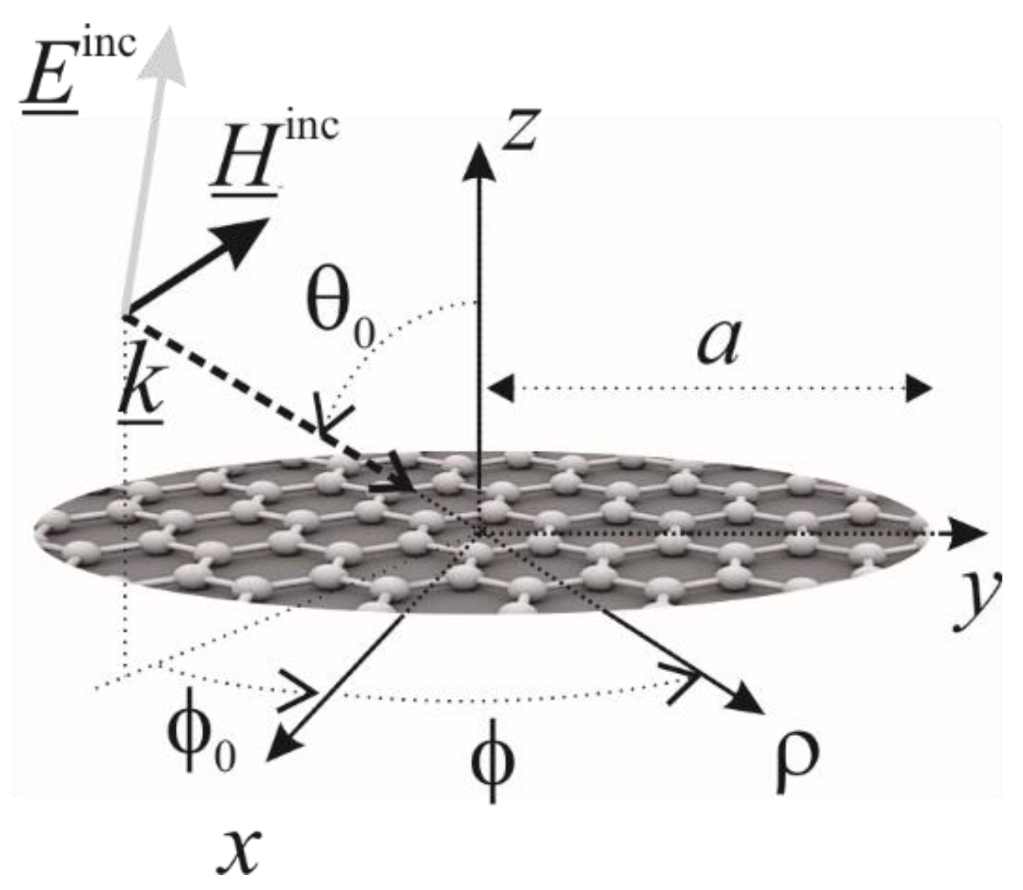
In Figure 1, a graphene disk of radius $a$ in free-space (with dielectric permittivity ${\epsilon }_0$ and magnetic permeability ${\mu }_0$), a Cartesian coordinate system $\left(x,y,z\right)$ and a cylindrical coordinate system $\left(\rho ,\varphi ,z\right)$, with the origin at the center of the disk and the z axis orthogonal to it, are sketched. The symbols $\lambda$, $f$, $\omega =2\pi f$, $k_0=2\pi /\lambda =\omega \sqrt{{\epsilon }_0{\mu }_0}$ and $Z_0=\sqrt{{\mu }_0/{\epsilon }_0}$ denote, respectively, the free-space wavelength, the frequency, the angular frequency, the free-space wavenumber and the intrinsic impedance of free-space. An impinging plane-wave of electric and magnetic fields given by ${\underset{\_}{E}}^{\mathrm{inc}} \left(\underset{\_}{r}\right) = {\underset{\_}{E}}_0{e}^{- \mathrm{j}\underset{\_}{k}\cdot \underset{\_}{r}}$ and ${\underset{\_}{H}}^{\mathrm{inc}} \left(\underset{\_}{r}\right) = {\underset{\_}{H}}_0{e}^{- \mathrm{j}\underset{\_}{k}\cdot \underset{\_}{r}} = \widehat{k}\times {\underset{\_}{E}}_0{e}^{- \mathrm{j}\underset{\_}{k}\cdot \underset{\_}{r}}/Z_0$, respectively, where $\underset{\_}{r}=\left(\rho ,\varphi ,z\right)$, $\underset{\_}{k}=-k_0\left(\sin {\theta }_0\cos \left({\varphi }_0-\varphi \right)\widehat{\rho }+\sin {\theta }_0\sin \left({\varphi }_0-\varphi \right)\widehat{\varphi }+\cos {\theta }_0\widehat{z}\right)$ and $\widehat{k}=\underset{\_}{k}/k_0$, excites a surface current density on the disk surface, $\underset{\_}{J}\left(\rho ,\varphi \right)$, generating a scattered field, $\left({\underset{\_}{E}}^{\mathrm{sc}}\left(\underset{\_}{r}\right),{\underset{\_}{H}}^{\mathrm{sc}}\left(\underset{\_}{r}\right)\right)$. Let us denote the total field, given by the sum of the incident field and the scattered field, by $\left(\underset{\_}{E}\left(\underset{\_}{r}\right),\underset{\_}{H}\left(\underset{\_}{r}\right)\right)$.

Thinking of the graphene disk as an impedance surface, the electromagnetic analysis can be approached by properly defining the corresponding impedance level, due to the graphene surface conductivity. Supposing to consider a disk with a radius larger than 50 nm, the edge effects on the graphene surface conductivity, which appear when the dimensions of the structure are smaller than 100 nm, can be neglected, i.e., the electrical conductivity model developed for an infinite graphene sheet can be used [53]. Moreover, supposing not to apply a magnetic bias field, the graphene can be assumed to be isotropic. Hence, according to the Kubo formalism [22], the surface conductivity of the graphene, ${\sigma }_s$, can be expressed as follows:

$${\sigma }_s={\sigma }_{intra}+{\sigma }_{inter},$$

(1a)

$${\sigma }_{intra}=-j\frac{e^2{k}_{B}T}{\pi {\hslash }^2\left(\omega -j/t_{relax}\right)}\left(\frac{{\mu }_c}{k_{B}T}+2\ln \left(e^{-\frac{{\mu }_c}{k_{B}T}}+1\right)\right),$$

(1b)

$${\sigma }_{inter} = - j\frac{e^2\left(\omega - j/t_{relax}\right)}{\pi {\hslash }^2}{\displaystyle \underset{0}{\overset{+\infty }{\int }}\frac{f_d\left(-\epsilon \right)-f_d\left(\epsilon \right)}{{\left(\omega - j/t_{relax}\right)}^2 -4{\left(\epsilon /\hslash \right)}^2}d\epsilon },$$

(1c)

$$f_d\left(\epsilon \right)=1/\left(e^{\frac{\epsilon -{\mu }_c}{k_{B}T}}+1\right),$$

(1d)

where ${\sigma }_{intra}$ is due to the intraband contributions while ${\sigma }_{inter}$ is related to the interband transitions, $e$ is the electron charge, $k_B$ is the Boltzmann constant, T is the temperature, $\hslash$ is the reduced Planck constant, $t_{relax}$ is the relaxation time of an electron, and ${\mu }_c$ is the chemical potential.

By imposing the impedance boundary condition on the disk surface [54,55], i.e.,

$$\widehat{z}\times \left(\underset{\_}{E}\left(\rho ,\varphi ,0^{+}\right)+\underset{\_}{E}\left(\rho ,\varphi ,0^{-}\right)\right)\times \widehat{z}=2R\underset{\_}{J}\left(\rho ,\varphi \right)$$

(2)

for $\rho \le a$ and $0\le \varphi <2\pi$, where $R=1/{\sigma }_s$ is the (complex) surface resistivity of the graphene, a boundary value problem for the Maxwell equations is obtained, which is uniquely solvable providing that the power boundedness condition and the Silver-Muller radiation condition are satisfied [25,56].

According to the second Green formula, the scattered electric field can be written in the form of a convolution integral involving the surface current density, the Green’s function of the problem, and their normal to the disk derivatives. A suitable choice of the Green’s function allows to automatically satisfy the radiation condition, while a proper definition of the behavior of the surface current density at the disk rim ensures the finite energy in any bounded domain including the edge. A surface integral equation for the surface current density can be obtained by substituting the obtained integral expression of the scattered electric field in Equation (2).

By expanding the fields in Fourier series, the revolution symmetry of the problem allows to recast the obtained integral equation to an infinite set of independent one-dimensional singular integral equations in the Hankel transform domain [50]. For the n-th harmonic, the integral equation can be written as follows:

$${\displaystyle \underset{0}{\overset{+\infty }{\int }}{\underset{\_}{\underset{\_}{H}}}^{\left(n\right)}\left(w\rho \right)\underset{\_}{\underset{\_}{\tilde{\overline{G}}}}\left(w\right){\underset{\_}{\tilde{J}}}^{\left(n\right)}\left(w\right)wdw}=-{\underset{\_}{E}}^{\mathrm{inc}\left(n\right)}\left(\rho ,0\right)$$

(3)

for $\rho \le a$, where

$${\underset{\_}{\tilde{J}}}^{\left(n\right)}\left(w\right)=\left(\begin{array}{c}{\tilde{J}}_{\mathrm{C}}\left(w\right)\\ -\mathrm{j}{\tilde{J}}_D\left(w\right)\end{array}\right)={\displaystyle \underset{0}{\overset{+\infty }{\int }}{\underset{\_}{\underset{\_}{H}}}^{\left(n\right)}\left(w\rho \right)}{\underset{\_}{J}}^{\left(n\right)}\left(\rho \right)\rho d\rho$$

(4)

is the vector Hankel transform of order n (VHT_n) of the n-th harmonic of the surface current density [57],

$${\underset{\_}{J}}^{\left(n\right)}\left(\rho \right)=\left(\begin{array}{c}{J}_{\rho }^{\left(n\right)}\left(\rho \right)\\ -\mathrm{j}{J}_{\varphi }^{\left(n\right)}\left(\rho \right)\end{array}\right),$$

(5)

the kernel of the VHT_n is denoted by

$${\underset{\_}{\underset{\_}{H}}}^{\left(n\right)}\left(w\rho \right)=\left(\begin{array}{cc}{J^{\prime }}_n\left(w\rho \right)& n{J}_n\left(w\rho \right)/\left(w\rho \right)\\ n{J}_n\left(w\rho \right)/\left(w\rho \right)& {J^{\prime }}_n\left(w\rho \right)\end{array}\right),$$

(6)

where $J_n(\cdot )$ and ${J^{\prime }}_n(\cdot )$ are the Bessel function of the first kind and order n and its first derivative with respect to the argument, respectively [58],

$$\underset{\_}{\underset{\_}{\tilde{\overline{G}}}}\left(w\right)=\underset{\_}{\underset{\_}{\tilde{G}}}\left(w\right)-R\underset{\_}{\underset{\_}{I}},$$

(7)

where

$$\underset{\_}{\underset{\_}{\tilde{G}}}\left(w\right)=\frac{1}{2\omega {\epsilon }_0}\left(\begin{array}{cc}-\sqrt{k_0^2-w^2}& 0\\ 0& -k_0^2/\sqrt{k_0^2-w^2}\end{array}\right)$$

(8)

with $\sqrt{k_0^2-w^2}=-\mathrm{j}\hspace{0.17em}\sqrt{-k_0^2+w^2}$ is the well-known spectral domain Green’s function of the problem at hand, $\underset{\_}{\underset{\_}{I}}$ is the identity matrix, and

$${\underset{\_}{E}}^{\mathrm{inc}\left(n\right)}\left(\rho ,0\right)=\left(\begin{array}{c}{E}_{\rho }^{\mathrm{inc}\left(n\right)}\left(\rho ,0\right)\\ -\mathrm{j}{E}_{\varphi }^{\mathrm{inc}\left(n\right)}\left(\rho ,0\right)\end{array}\right)$$

(9)

is the n-th harmonic of the incident electric field in the disk plane.

It is simple to demonstrate that the following functions:

$${\mathrm{VHT}}_n^{-1}\left[\left(\begin{array}{c}{\tilde{J}}_{\mathrm{C}}^{\left(n\right)}\left(w\right)\\ 0\end{array}\right)\right]=\left(\begin{array}{c}\frac{d}{d\rho }\\ \frac{n}{\rho }\end{array}\right){\Phi }_{\mathrm{C}}^{\left(n\right)}\left(\rho \right),$$

(10a)

$${\mathrm{VHT}}_n^{-1}\left[\left(\begin{array}{c}0\\ -\mathrm{j}\hspace{0.17em}{\tilde{J}}_{\mathrm{D}}^{\left(n\right)}\left(w\right)\end{array}\right)\right]=-\mathrm{j}\hspace{0.17em}\left(\begin{array}{c}\frac{n}{\rho }\\ \frac{d}{d\rho }\end{array}\right){\Phi }_{\mathrm{D}}^{\left(n\right)}\left(\rho \right),$$

(10b)

where the symbol ${\mathrm{VHT}}_n^{-1}$ denotes the inverse vector Hankel transform of order n, are the surface curl-free contribution and the surface divergence-free contribution of the n-th harmonic of the surface current density, respectively, ${\Phi }_{r,T}^{\left(n\right)}\left(\rho \right)$ for $T=\mathrm{C},\mathrm{D}$ being suitable potential functions [59]. Hence, in order to deal with scalar unknowns in the spectral domain, such contributions are assumed as new unknowns.

According to MAP, the obtained integral equations are numerically solved by means of the Galerkin method. The key point is the proper selection of the expansion functions. Due to the behavior of the field at the disk rim [60] and the properties of the Fourier series expansion, the following behavior of the components of the n-th harmonic of the surface current density can be readily stated:

$$J_t^{\left(n\right)}\left(\rho \right)=\{\begin{array}{cc}{\rho }^{\left|\left|n\right|-1\right|}{\left(a-\rho \right)}^{p_t}{\overline{J}}_t^{\left(n\right)}\left(\rho \right)& \rho <a\\ 0& \rho >a\end{array},$$

(11)

for $t\in \left\{\rho ,\varphi \right\}$, where $p_{\rho }=1/2$, $p_{\varphi }=0$, and ${\overline{J}}_t^{\left(n\right)}\left(\rho \right)$ are well behaved functions because the sources are off the scatterer surface. By means of the procedure detailed in [48,49,50,51,52], it is possible to demonstrate that such a behavior can be reconstructed by expanding the functions ${\tilde{J}}_T^{\left(n\right)}\left(w\right)$ in the following complete and non-redundant Neumann series of weighted Bessel functions [61], orthonormal on the interval $\left(0,+\infty \right)$ with the weight function $w^{2p_T-1}$ (according to the Weber-Schafheitlin discontinuous integral [62]):

$${\tilde{J}}_T^{\left(n\right)}\left(w\right)={\displaystyle \sum _{h=-1+{\delta }_{n,0}}^{+\infty }{\gamma }_{T,h}^{\left(n\right)}\hspace{0.17em}\sqrt{2\left(\left|n\right|+2h+p_T+1\right)}\frac{J_{\left|n\right|+2h+p_T+1}\left(aw\right)}{w^{p_T}}},$$

(12a)

$${\gamma }_{D,-1}^{\left(n\right)}={\alpha }^{\left(n\right)}{\gamma }_{C,-1}^{\left(n\right)},$$

(12b)

$${\alpha }^{\left(n\right)}=\frac{j\mathrm{sgn}\left(n\right)\left|n\right|!}{\Gamma \left(\left|n\right|+3/2\right)}\sqrt{\frac{a\left(\left|n\right|+1/2\right)}{2\left|n\right|}},$$

(12c)

where ${\delta }_{n,m}$ is the Kronecker delta, ${\gamma }_{T,h}^{\left(n\right)}$ denotes the general expansion coefficient, and, for a graphene disk, $p_{\mathrm{C}}=3/2$ and $p_{\mathrm{D}}=1$. Hence, the selected sets of expansion functions, if used in a Galerkin scheme, diagonalize the most singular part of the integral operator (leading to the identity matrix operator), which is obtained by replacing $\underset{\_}{\underset{\_}{\tilde{\overline{G}}}}\left(w\right)$ in (3) with its asymptotic behavior, i.e.,

$$\underset{\_}{\underset{\_}{\tilde{\overline{G}}}}\left(w\right)\stackrel{w\to +\infty }{~}{\underset{\_}{\underset{\_}{\tilde{\overline{G}}}}}^{\infty }\left(w\right)=\left(\begin{array}{cc}\mathrm{j}\frac{w}{2\omega {\epsilon }_0}& 0\\ 0& -R\end{array}\right).$$

(13)

Moreover, it is possible to show that the discretized counterpart of the operator obtained by subtracting ${\underset{\_}{\underset{\_}{\tilde{\overline{G}}}}}^{\infty }\left(w\right)$ from $\underset{\_}{\underset{\_}{\tilde{\overline{G}}}}\left(w\right)$ is compact in $l^2$ [50]. Hence, the resulting matrix equation is of the Fredholm second-kind in $l^2$ because the free-term has a bounded $l^2$-norm [25].

3. Numerical Results and Discussion

In this section, for the sake of brevity, the SPRs excited by an orthogonally to the disk impinging plane wave (${\theta }_0=0$°) are analyzed. In such a case, only the harmonics for $n=\pm 1$ contribute to the representation of the fields. Hence, the attention is focused on SPRs with one variation of the fields along the disk azimuth. Moreover, the electric field is assumed directed along the y axis, i.e., ${\underset{\_}{E}}_0=E_0\widehat{y}$.

As detailed above, in order to characterize SPRs, parameters such as TSCS and ACS are very useful and handy tools. Indeed, the resonance frequencies can be individuated by the position of the peaks of such parameters for varying values of the frequency. Moreover, as shown in the following, they can be expressed in closed form.

Using the stationary phase method, the far scattered electric field can be expressed in closed form as [56]

$$E_s^{\mathrm{sc}}\left(r,\theta ,\varphi \right)\stackrel{r\to +\infty }{\sim }\frac{e^{- \mathrm{j}\hspace{0.17em}{k}_{0}r}}{r}{F}_s\left(\theta ,\varphi \right)$$

(14)

with $s=\theta ,\varphi$, where

$$F_{\theta }\left(\theta ,\varphi \right)=- \frac{\omega {\mu }_0}{2}\cos \theta {\displaystyle \sum _{n=-\infty }^{+\infty }{e}^{\mathrm{j}\hspace{0.17em}n\left(\varphi + \frac{\pi }{2}\right)} {\tilde{J}}_{\mathrm{C}}^{\left(n\right)} \left(k_0\sin \theta \right)},$$

(15a)

$$F_{\varphi } \left(\theta ,\varphi \right)=- \frac{\omega {\mu }_0}{2} {\displaystyle \sum _{n=- \infty }^{+\infty }{e}^{\mathrm{j}\hspace{0.17em}n\left(\varphi + \frac{\pi }{2}\right)} {\tilde{J}}_{\mathrm{D}}^{\left(n\right)} \left(k_0\sin \theta \right)}.$$

(15b)

TSCS and ACS are defined as follows:

$${\sigma }_{\mathrm{TSCS}}=\frac{1}{{\left|{\underset{\_}{E}}_0\right|}^2}{\displaystyle \underset{0}{\overset{\pi }{\int }}{\displaystyle \underset{0}{\overset{2\pi }{\int }}{\left|\underset{\_}{F}\left(\theta ,\varphi \right)\right|}^2\sin \theta d\varphi d\theta }},$$

(16a)

$${\sigma }_{\mathrm{ACS}}=\frac{P^{\mathrm{abs}}}{{\left|{\underset{\_}{E}}_0\right|}^2/\left(2Z_0\right)}= \frac{2\pi Z_0\Re \left\{R\right\}}{{\left|{\underset{\_}{E}}_0\right|}^2} {\displaystyle \sum _{n=-\infty }^{+\infty }{\displaystyle \underset{0}{\overset{a}{\int }}{\left|{\underset{\_}{J}}^{\left(n\right)}\left(\rho \right)\right|}^2\rho d \rho }},$$

(16b)

where $P^{\mathrm{abs}}$ is the power absorbed by the graphene disk and $\Re \{\cdot \}$ denotes the real part of a complex number.

According to the Parseval’s formula [63],

$${\displaystyle \underset{0}{\overset{a}{\int }}{\left|{\underset{\_}{J}}^{\left(n\right)}\left(\rho \right)\right|}^2\rho d \rho }={\displaystyle \underset{0}{\overset{+\infty }{\int }}{\left|{\underset{\_}{\tilde{J}}}_{\mathrm{C}}^{\left(n\right)}\left(w\right)\right|}^{2}wdw}+{\displaystyle \underset{0}{\overset{+\infty }{\int }}{\left|{\underset{\_}{\tilde{J}}}_{\mathrm{D}}^{\left(n\right)}\left(w\right)\right|}^{2}wdw},$$

(17)

which can be expressed in closed form by substituting (12a) in (17) and using the Weber-Schafheitlin discontinuous integral. Hence, ACS is expressed in closed form. Moreover, since TSCS and ACS are related to each other by means of the forward scattering theorem [64], i.e.,

$${\sigma }_{\mathrm{TSCS}}+{\sigma }_{\mathrm{ACS}}=-\frac{4\pi }{k_0{\left|{\underset{\_}{E}}_0\right|}^2}\Im \left\{{\underset{\_}{E}}_0^{\ast }\cdot \underset{\_}{F}\left(\pi -{\theta }_0,\pi +{\varphi }_0\right)\right\}$$

(18)

where $\Im \{\cdot \}$ denotes the imaginary part of a complex number, even TSCS admits a closed form expression.

In order to establish a convergence criterion for the truncated version of the obtained Fredholm second-kind matrix operator equation, the following normalized truncation error is introduced:

$${err}_N\left(M\right)=\sqrt{{\displaystyle \sum _{n=-N+1}^{N-1}\hspace{1em}{\Vert x_{M+1}^{\left(n\right)}-x_M^{\left(n\right)}\Vert }^2}/{\displaystyle \sum _{n=-N+1}^{N-1}\hspace{1em}{\Vert x_M^{\left(n\right)}\Vert }^2}}$$

(19)

where, in our case, $N=2$, $\Vert \cdot \Vert$ is the usual Euclidean norm and $x_M^{\left(n\right)}$ is a vector related to the first M expansion coefficients of ${\underset{\_}{\tilde{J}}}_T^{\left(n\right)}\left(w\right)$ [50]. Since $\underset{M\to +\infty }{\lim }{\mathrm{err}}_N\left(M\right)=0$, in the examples detailed in the following M will be chosen in order to guarantee that ${\mathrm{err}}_N\left(M\right)<{10}^{-2}$ definitely. As stated above, the proposed method is fast convergent. Indeed, for the cases examined in this paper, at most 8 expansion functions for each unknown are needed to reconstruct the solution. The proposed method is very efficient even in terms of computation time as at most 2s are needed to reconstruct the solution by means of an in-house C++ software code running on a laptop equipped with an Intel Core i7-10510U 1.8 GHz, 16 GB RAM. For the sake of completeness, it is worth mentioning that the implemented software code has been checked in [50] by means of comparisons with the general-purpose commercial software CST Microwave Studio (CST-MWS) showing a very good agreement. Moreover, the comparisons provided in [50] demonstrate the effectiveness of the proposed method, which drastically outperforms CST-MWS in terms of both computation time and storage requirement in all the examined cases.

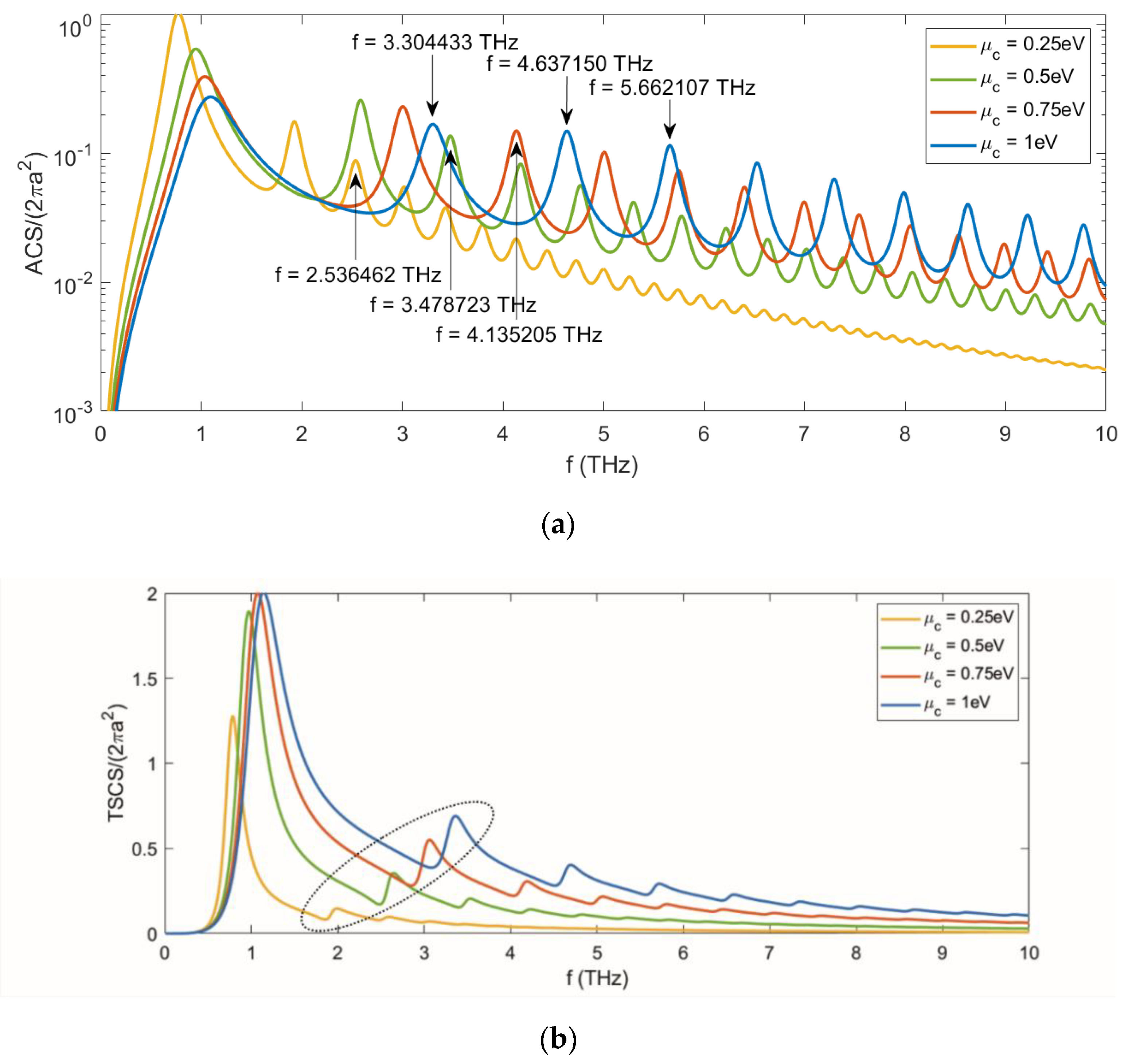
Figure 2 shows the normalized ACS and TSCS of the graphene disk with the radius $a=50 \mathsf{\mu }\mathrm{m}$ and the electron relaxation time $t_{relax}=1 \mathrm{ps}$, at the room temperature $T=300 \mathrm{K}$, for different values of the chemical potential ${\mu }_c=0.25 \mathrm{eV}, 0.5\mathrm{eV} , 0.75 \mathrm{eV}, 1 \mathrm{eV}$ and for varying values of the frequency. Many peaks can be observed in both the figures corresponding to the SPRs. In Figure 2a, the resonance frequencies discussed throughout this section are marked. Moreover, Figure 2b clearly shows that the resonance frequencies up-shift as the chemical potential increases (see, for example, the peaks circled in the figure).

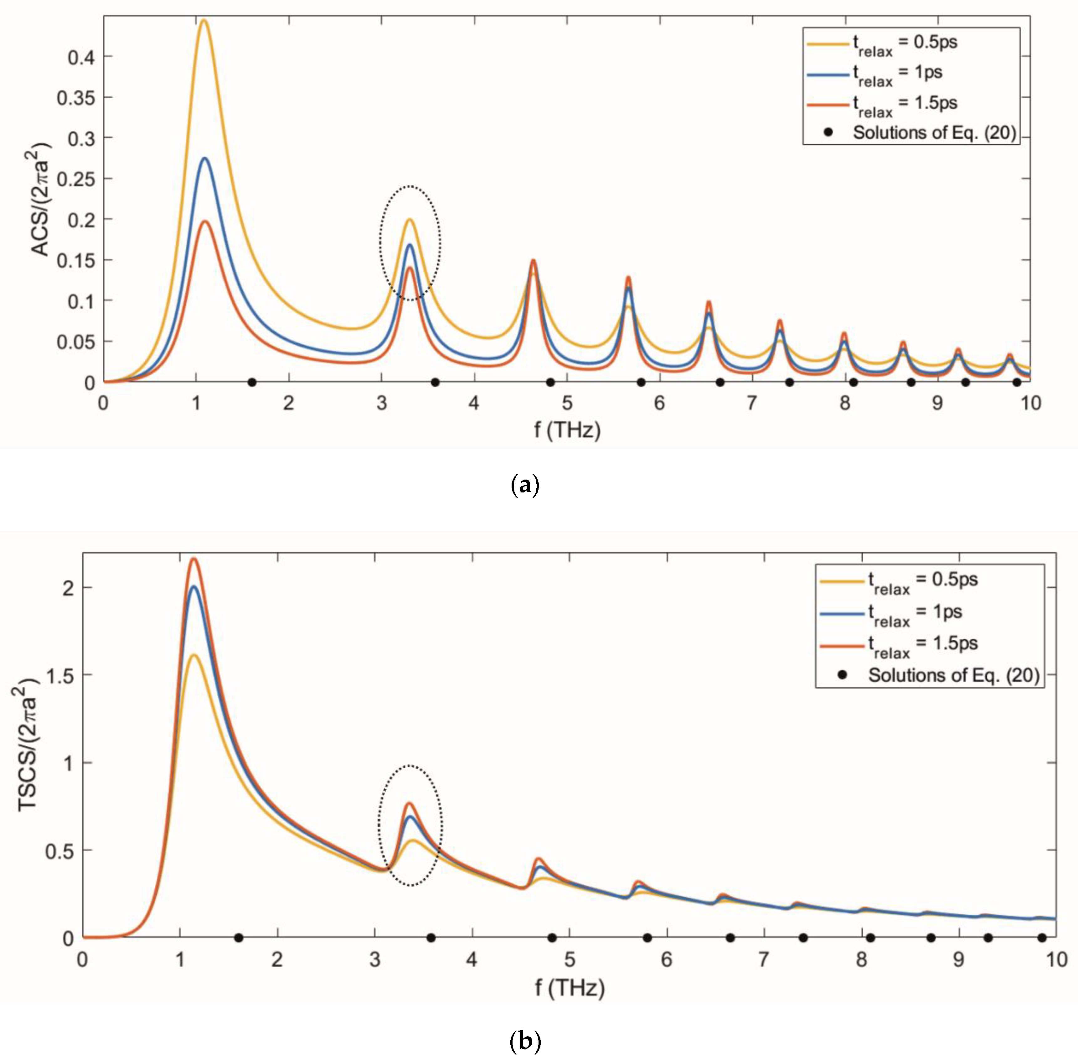
Figure 3 shows the normalized ACS and TSCS of the graphene disk with $a=50 \mathsf{\mu }\mathrm{m}$, and ${\mu }_c=1\mathrm{eV}$, at the room temperature $T=300 \mathrm{K}$, for different values of the electron relaxation time $t_{relax}=0.5\mathrm{ps},1\mathrm{ps},1.5\mathrm{ps}$ and for varying values of the frequency. As can be observed, the resonance frequencies are independent of the electron relaxation time (see, for example, the peaks circled in Figure 3). However, the peaks intensity changes from case to case due to the different dissipation losses.

It is interesting to observe that, according to [55,65,66], the obtained resonance frequencies can be estimated as the solution of the following approximate equation:

$$J_1^{\prime }\left(k_{0}a\hspace{0.17em}\Re \left\{\sqrt{1-{\left(\frac{2}{{\sigma }_s{Z}_0}\right)}^2}\right\}\right)\approx 0,$$

(20)

with an error which decreases as the frequency increases (see Figure 3).

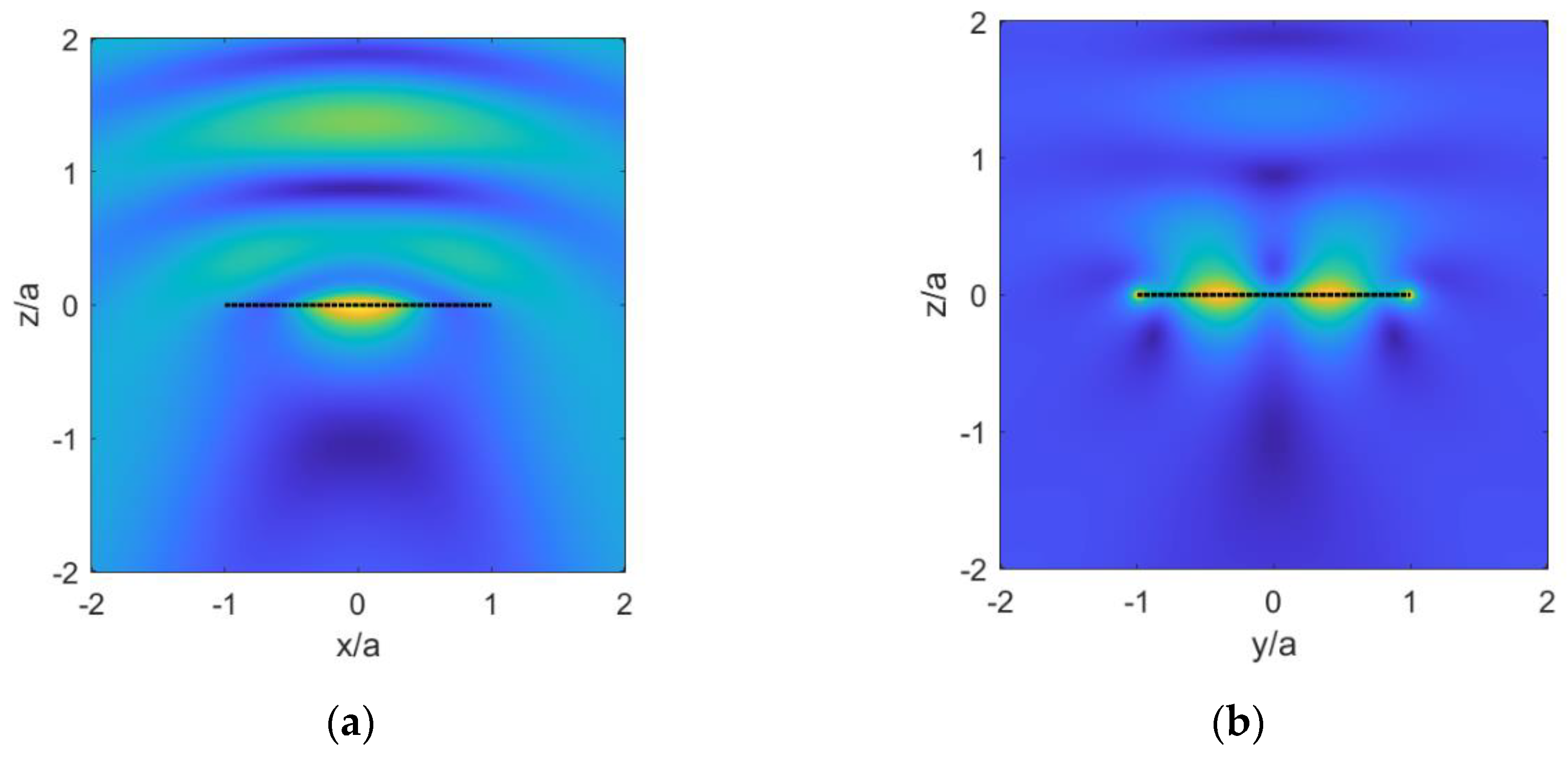
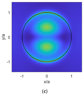
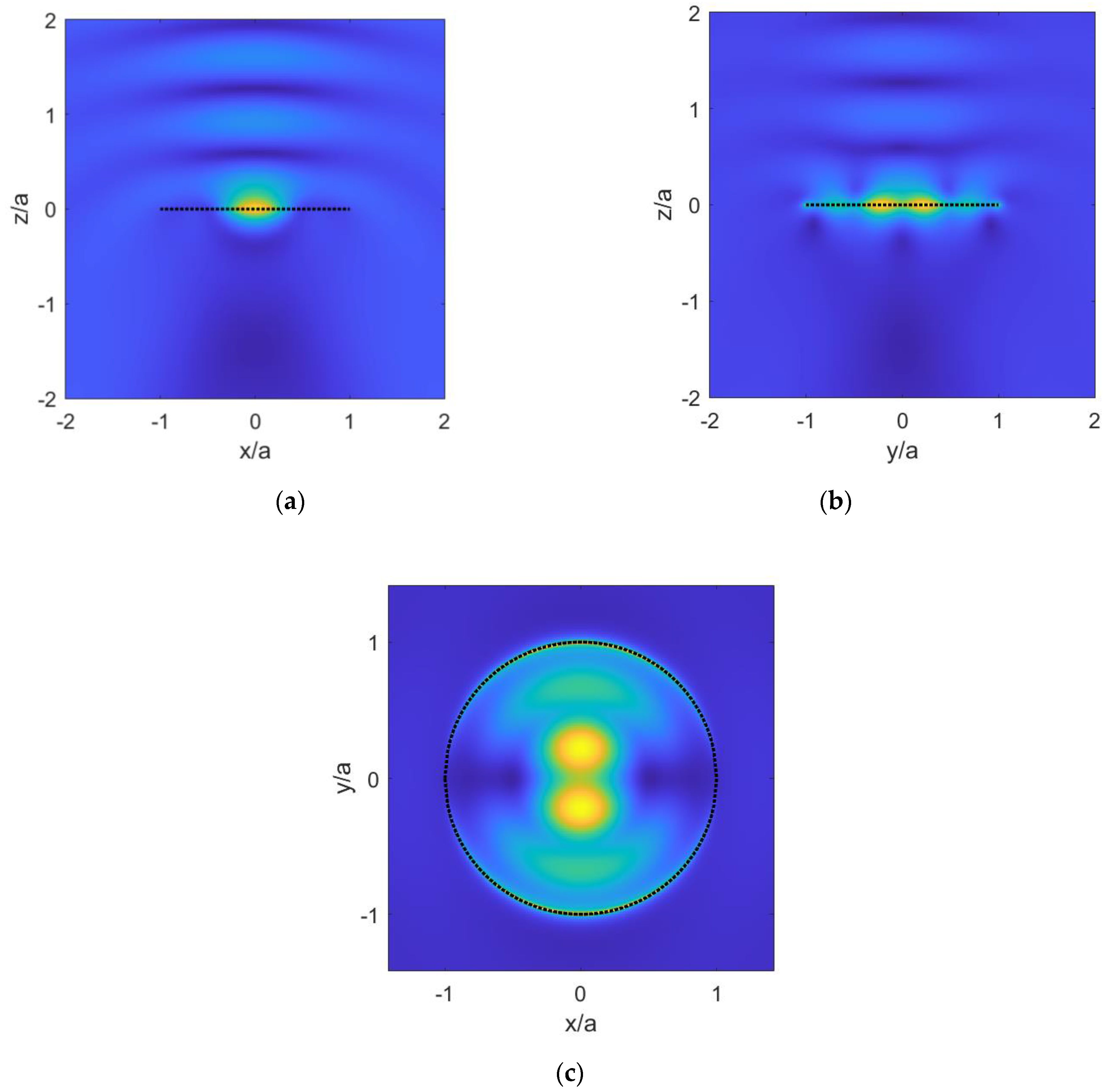
In Figure 4, the total electric field of the graphene disk with $a=50 \mathsf{\mu }\mathrm{m}$, $t_{relax}=1\mathrm{ps}$, $T=300 \mathrm{K}$, ${\mu }_c=1\mathrm{eV}$ is plotted in the near-field region at the resonance frequency $f=3.304433\mathrm{THz}$. As can be clearly seen, the SPR is formed as a Fabry–Pérot-like standing wave due to the reflection of the surface plasmon polariton at the disk rim. Moreover, a bright behavior due to the divergence of the electric field at the edge can be observed. Analogously, in Figure 5 and Figure 6, for the same disk, the near total electric field is plotted at the resonance frequencies $f=4.637150\mathrm{THz}$ and $f=5.662107\mathrm{THz}$, respectively. Now, two and three oscillations along the radial direction can be observed for the excited SPRs, respectively.

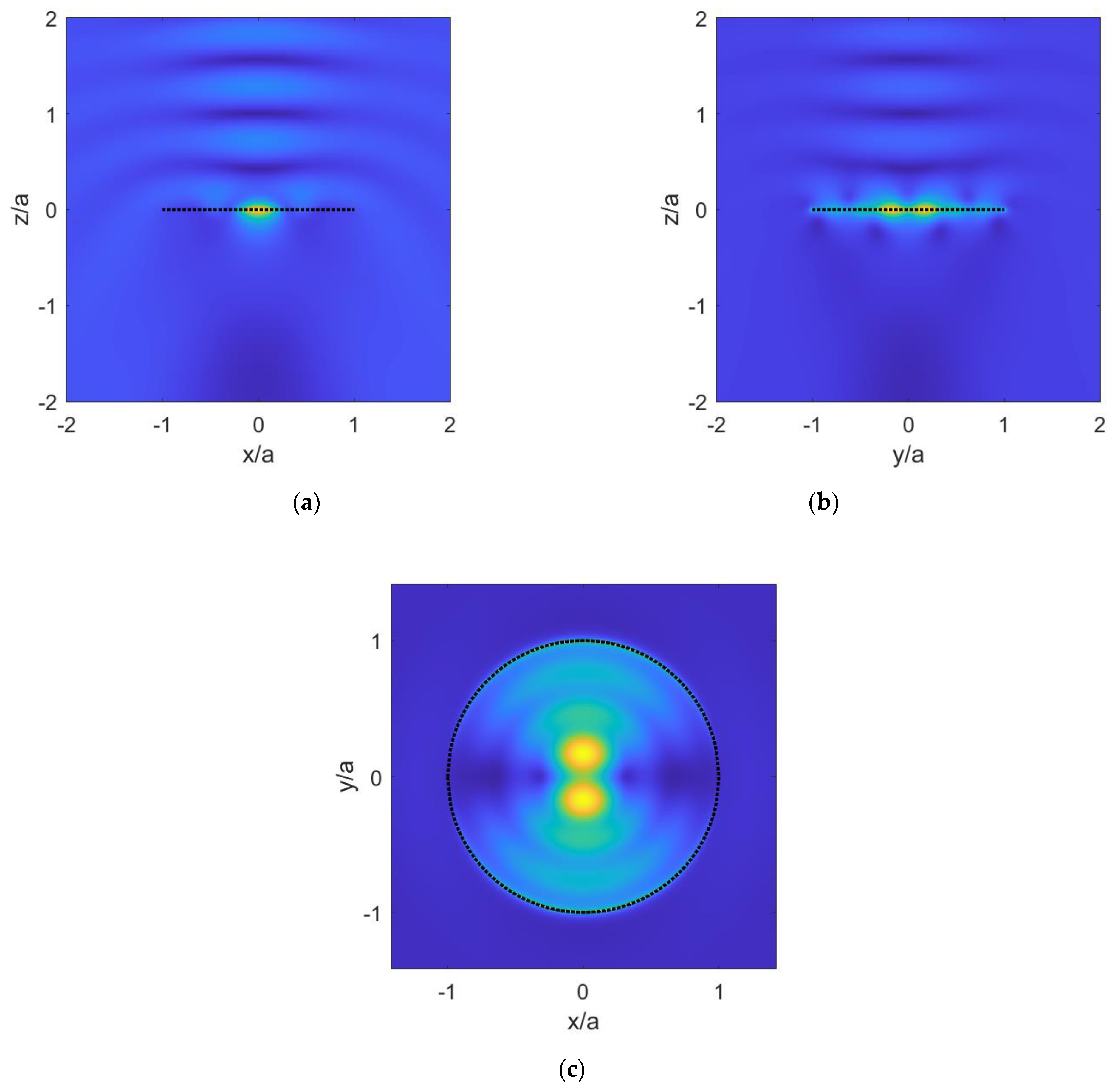
To conclude, in order to show that a change of the chemical potential simply results in a shift of the resonance frequencies, without a significant variation of the field behavior, in Figure 7, the near total electric field is shown for $a=50 \mathsf{\mu }\mathrm{m}$, $t_{relax}=1\mathrm{ps}$, $T=300 \mathrm{K}$, and for different values of the chemical potential, ${\mu }_c=0.25\mathrm{eV},0.5\mathrm{eV},0.75\mathrm{eV},1\mathrm{eV}$, at the resonance frequencies $f=2.536462\mathrm{THz},3.478723\mathrm{THz},4.135205\mathrm{THz},4.637150\mathrm{THz}$, respectively, corresponding to the standing waves with two oscillations along the radial direction. It is clear as the plotted fields are almost indistinguishable.

4. Conclusions

In this paper, the SPRs of a graphene disk were studied by means of a guaranteed- convergence method, based on the Helmholtz decomposition and MAP. The proposed method has revealed to be very efficient in terms of both computation time and storage requirement, confirming the very good results previously obtained in analyzing the electromagnetic scattering from PEC, resistive and dielectric disks. The SPRs were excited by an impinging plane wave and the resonance frequencies have been searched for the peaks of TSCS and ACS, which were simply evaluated by means of closed form expressions. The obtained numerical results confirm that the resonance frequencies shift-up by increasing the chemical potential of the graphene and show that, for orthogonal incidence, the field behavior resembles a cylindrical standing wave with one variation along the disk azimuth.

The proposed method can be readily generalized to analyze arrays of graphene disks in homogeneous and layered media. Further generalizations of the method for the analysis of composite graphene-dielectric disks, graphene annular rings, finite-length graphene nano-tubes and cylindrical arcs are being worked on.

References

- Berger, C.; Song, Z.; Li, T.; Li, X.; Ogbazghi, A.Y.; Feng, R.; Dai, Z.; Marchenkov, A.N.; Conrad, E.H.; First, P.N.; et al. Ultrathin epitaxial graphite: 2D electron gas properties and a route toward graphene-based nanoelectronics. J. Phys. Chem. B 2004, 108, 19912–19916. [Google Scholar] [CrossRef] [Green Version]
- Geim, K.; Novoselov, K.S. The rise of graphene. Nat. Mater. 2007, 6, 183–191. [Google Scholar] [CrossRef]
- Gusynin, V.P.; Sharapov, S.G.; Carbotte, J.P. Magnetooptical conductivity in graphene. J. Phys. Condens. Matter 2007, 19, 026222. [Google Scholar] [CrossRef] [Green Version]
- Lee, C.; Wei, X.; Kysar, J.W.; Hone, J. Measurement of the elastic properties and intrinsic strength of monolayer graphene. Science 2008, 321, 385–388. [Google Scholar] [CrossRef]
- Castro Neto, A.H.; Guinea, F.; Peres, N.M.R.; Novoselov, K.S.; Geim, A.K. The electronic properties of graphene. Rev. Mod. Phys. 2009, 81, 109–162. [Google Scholar] [CrossRef] [Green Version]
- Zhu, Y.; Murali, S.; Cai, W.; Li, X.; Suk, J.W.; Potts, J.R.; Ruoff, R.S. Graphene and graphene oxide: Synthesis, properties, and applications. Adv. Mater. 2010, 22, 3906–3924. [Google Scholar] [CrossRef]
- Balandin, A.A. Thermal properties of graphene and nanostructured carbon materials. Nat. Mater. 2011, 10, 569–581. [Google Scholar] [CrossRef] [PubMed] [Green Version]
- Grigorenko, A.N.; Polini, M.; Novoselov, K.S. Graphene plasmonics. Nat. Photonics 2012, 6, 749–758. [Google Scholar] [CrossRef]
- Wang, X.; Zhi, L.; Mullen, K. Transparent, conductive graphene electrodes for dye-sensitized solar cells. Nano Lett. 2008, 8, 323–327. [Google Scholar] [CrossRef] [PubMed]
- Rana, F. Graphene terahertz plasmon oscillators. IEEE Trans. Nanotechnol. 2008, 7, 91–99. [Google Scholar] [CrossRef] [Green Version]
- Jablan, M.; Buljan, H.; Soljacic, M. Plasmonics in graphene at infrared frequencies. Phys. Rev. B 2009, 80, 245435. [Google Scholar] [CrossRef] [Green Version]
- Schwierz, F. Graphene transistors. Nat. Nanotechnol. 2010, 5, 487–496. [Google Scholar] [CrossRef] [PubMed]
- Crassee, I.; Levallois, J.; Walter, A.L.; Ostler, M.; Bostwick, A.; Rotenberg, E.; Seyller, T.; van der Marel, D.; Kuzmenko, A.B. Giant Faraday rotation in single-and multilayer graphene. Nat. Phys. 2011, 7, 48–51. [Google Scholar] [CrossRef] [Green Version]
- Chen, P.Y.; Alù, A. Atomically thin surface cloak using graphene monolayers. ACS Nano 2011, 5, 5855–5863. [Google Scholar] [CrossRef]
- Vakil, A.; Engheta, N. Transformation optics using graphene. Science 2012, 332, 1291–1294. [Google Scholar] [CrossRef] [Green Version]
- Sensale-Rodriguez, B.; Yan, R.; Kelly, M.M.; Fang, T.; Tahy, K.; Hwang, W.S.; Jena, D.; Liu, L.; Xing, H.G. Broadband graphene terahertz modulators enabled by intraband transitions. Nat. Commun. 2012, 3, 780. [Google Scholar] [CrossRef] [PubMed]
- Chen, P.Y.; Argyropoulos, C.; Alù, A. Terahertz antenna phase shifters using integrally-gated graphene transmission-lines. IEEE Trans. Antennas Propag. 2013, 61, 1528–1537. [Google Scholar] [CrossRef] [Green Version]
- Gómez-Díaz, J.S.; Perruisseau-Carrier, J. Graphene-based plasmonic switches at near infrared frequencies. Opt. Express 2013, 21, 15490–15504. [Google Scholar] [CrossRef] [PubMed] [Green Version]
- Correas-Serrano, D.; Gomez-Diaz, J.S.; Perruisseau-Carrier, J.; Alvarez-Melcon, A. Graphene-based plasmonic tunable low-pass filters in the terahertz band. IEEE Trans. Nanotechnol. 2014, 13, 1145–1153. [Google Scholar] [CrossRef] [Green Version]
- Chu, D.A.; Hon, P.W.C.; Itoh, T.; Williams, B.S. Feasibility of graphene CRLH metamaterial waveguides and leaky wave antennas. J. Appl. Phys. 2016, 120, 013103. [Google Scholar] [CrossRef] [Green Version]
- Nag, A.; Mitra, A.; Mukhopadhyay, S.C. Graphene and its sensor-based applications: A review. Sens. Actuator A Phys. 2018, 270, 177–194. [Google Scholar] [CrossRef]
- Hanson, G.W. Dyadic Green’s functions for an anisotropic, non-local model of biased graphene. IEEE Trans. Antennas Propag. 2008, 56, 747–757. [Google Scholar] [CrossRef]
- Balaban, M.V.; Shapoval, O.V.; Nosich, A.I. THz wave scattering by a graphene strip and a disk in the free space: Integral equation analysis and surface plasmon resonances. J. Opt. 2013, 15, 114007. [Google Scholar] [CrossRef]
- Shapoval, O.V.; Gomez-Diaz, J.S.; Perruisseau-Carrier, J.; Mosig, J.R.; Nosich, A.I. Integral equation analysis of plane wave scattering by coplanar graphene-strip gratings in the THz range. IEEE Trans. Terahertz Sci. Technol. 2013, 3, 666–674. [Google Scholar] [CrossRef] [Green Version]
- Nosich, A.I. Method of analytical regularization in computational photonics. Radio Sci. 2016, 51, 1421–1430. [Google Scholar] [CrossRef]
- Kantorovich, L.V.; Akilov, G.P. Functional Analysis, 2nd ed.; Pergamon Press: Oxford, UK; Elmsford, NY, USA, 1982. [Google Scholar]
- Eswaran, K. On the solutions of a class of dual integral equations occurring in diffraction problems. Proc. R. Soc. Lond. Ser. A 1990, 429, 399–427. [Google Scholar]
- Veliev, E.I.; Veremey, V.V. Numerical-analytical approach for the solution to the wave scattering by polygonal cylinders and flat strip structures. In Analytical and Numerical Methods in Electromagnetic Wave Theory; Hashimoto, M., Idemen, M., Tretyakov, O.A., Eds.; Science House: Tokyo, Japan, 1993. [Google Scholar]
- Davis, M.J.; Scharstein, R.W. Electromagnetic plane wave excitation of an open-ended finite-length conducting cylinder. J. Electromagn. Waves Appl. 1993, 7, 301–319. [Google Scholar] [CrossRef]
- Hongo, K.; Serizawa, H. Diffraction of electromagnetic plane wave by rectangular plate and rectangular hole in the conducting plate. IEEE Trans. Antennas Propag. 1999, 47, 1029–1041. [Google Scholar] [CrossRef]
- Bliznyuk, N.Y.; Nosich, A.I.; Khizhnyak, A.N. Accurate computation of a circular-disk printed antenna axisymmetrically excited by an electric dipole. Microw. Opt. Technol. Lett. 2000, 25, 211–216. [Google Scholar] [CrossRef]
- Tsalamengas, J.L. Rapidly converging direct singular integral-equation techniques in the analysis of open microstrip lines on layered substrates. IEEE Trans. Microw. Theory Tech. 2001, 49, 555–559. [Google Scholar] [CrossRef]
- Losada, V.; Boix, R.R.; Medina, F. Fast and accurate algorithm for the short-pulse electromagnetic scattering from conducting circular plates buried inside a lossy dispersive half-space. IEEE Trans. Geosci. Remote Sens. 2003, 41, 988–997. [Google Scholar] [CrossRef]
- Hongo, K.; Naqvi, Q.A. Diffraction of electromagnetic wave by disk and circular hole in a perfectly conducting plane. Prog. Electromagn. Res. 2007, 68, 113–150. [Google Scholar] [CrossRef] [Green Version]
- Coluccini, G.; Lucido, M.; Panariello, G. Spectral domain analysis of open single and coupled microstrip lines with polygonal cross-section in bound and leaky regimes. IEEE Trans. Microw. Theory Tech. 2013, 61, 736–745. [Google Scholar] [CrossRef]
- Lucido, M. Electromagnetic scattering by a perfectly conducting rectangular plate buried in a lossy half-space. IEEE Trans. Geosci. Remote Sens. 2014, 52, 6368–6378. [Google Scholar] [CrossRef]
- Lucido, M.; Panariello, G.; Schettino, F. An EFIE formulation for the analysis of leaky-wave antennas based on polygonal cross-section open waveguides. IEEE Antennas Wirel. Propag. Lett. 2014, 13, 983–986. [Google Scholar] [CrossRef]
- Lucido, M. Complex resonances of a rectangular patch in a multilayered medium: A new accurate and efficient analytical technique. Prog. Electromagn. Res. 2014, 145, 123–132. [Google Scholar] [CrossRef] [Green Version]
- Lucido, M. Scattering by a tilted strip buried in a lossy half-space at oblique incidence. Prog. Electromagn. Res. M 2014, 37, 51–62. [Google Scholar] [CrossRef] [Green Version]
- Corsetti, F.; Lucido, M.; Panariello, G. Effective analysis of the propagation in coupled rectangular-core waveguides. IEEE Photon. Technol. Lett. 2014, 26, 1855–1858. [Google Scholar] [CrossRef]
- Lucido, M.; Panariello, G.; Pinchera, D.; Schettino, F. Cut-off wavenumbers of polygonal cross section waveguides. IEEE Microw. Wirel. Compon. Lett. 2014, 24, 656–658. [Google Scholar] [CrossRef]
- Lucido, M.; Migliore, M.D.; Pinchera, D. A new analytically regularizing method for the analysis of the scattering by a hollow finite-length PEC circular cylinder. Prog. Electromagn. Res. B 2016, 70, 55–71. [Google Scholar] [CrossRef] [Green Version]
- Lucido, M.; Di Murro, F.; Panariello, G.; Santomassimo, C. Fast converging CFIE-MoM analysis of electromagnetic scattering from PEC polygonal cross-section closed cylinders. Prog. Electromagn. Res. B 2017, 74, 109–121. [Google Scholar] [CrossRef] [Green Version]
- Lucido, M.; Schettino, F.; Migliore, M.D.; Pinchera, D.; Di Murro, F.; Panariello, G. Electromagnetic scattering by a zero-thickness PEC annular ring: A new highly efficient MoM solution. J. Electromagn. Waves Appl. 2017, 31, 405–416. [Google Scholar] [CrossRef]
- Lucido, M.; Santomassimo, C.; Panariello, G. The method of analytical preconditioning in the analysis of the propagation in dielectric waveguides with wedges. J. Light. Technol. 2018, 36, 2925–2932. [Google Scholar] [CrossRef]
- Lucido, M.; Migliore, M.D.; Nosich, A.I.; Panariello, G.; Pinchera, D.; Schettino, F. Efficient evaluation of slowly converging integrals arising from MAP application to a spectral-domain integral equation. Electronics 2019, 8, 1500. [Google Scholar] [CrossRef] [Green Version]
- Lucido, M. Analysis of the propagation in high-speed interconnects for MIMICs by means of the method of analytical preconditioning: A new highly efficient evaluation of the coefficient matrix. Appl. Sci. 2021, 11, 933. [Google Scholar] [CrossRef]
- Lucido, M.; Panariello, G.; Schettino, F. Scattering by a zero-thickness PEC disk: A new analytically regularizing procedure based on Helmholtz decomposition and Galerkin method. Radio Sci. 2017, 52, 2–14. [Google Scholar] [CrossRef]
- Lucido, M.; Di Murro, F.; Panariello, G. Electromagnetic scattering from a zero-thickness PEC disk: A note on the Helmholtz-Galerkin analytically regularizing procedure. Progr. Electromagn. Res. Lett. 2017, 71, 7–13. [Google Scholar] [CrossRef]
- Lucido, M.; Schettino, F.; Panariello, G. Scattering from a thin resistive disk: A guaranteed fast convergence technique. IEEE Trans. Antennas Propag. 2021, 69, 387–396. [Google Scholar] [CrossRef]
- Lucido, M.; Balaban, M.V.; Dukhopelnykov, S.V.; Nosich, A.I. A fast-converging scheme for the electromagnetic scattering from a thin dielectric disk. Electronics 2020, 9, 1451. [Google Scholar] [CrossRef]
- Lucido, M.; Balaban, M.V.; Nosich, A.I. Plane wave scattering from thin dielectric disk in free space: Generalized boundary conditions, regularizing Galerkin technique and whispering gallery mode resonances. IET Microw. Antennas Propag. 2021. [Google Scholar] [CrossRef]
- Han, M.Y.; Özyilmaz, B.; Zhang, Y.; Kim, P. Energy band-gap engineering of graphene nanoribbons. Phys. Rev. Lett. 2007, 98, 206805. [Google Scholar] [CrossRef] [Green Version]
- Bleszynski, E.; Bleszynski, M.; Jaroszewicz, T. Surface-integral equations for electrmagnetic scattering from impenetrable and penetrable sheets. IEEE Antennas Propag. Mag. 1993, 35, 14–24. [Google Scholar] [CrossRef]
- Balaban, M.V.; Sauleau, R.; Benson, T.M.; Nosich, A.I. Dual integral equations technique in electromagnetic scattering by a thin disk. Prog. Electromagn. Res. B 2009, 16, 107–126. [Google Scholar] [CrossRef] [Green Version]
- Jones, D.S. The Theory of Electromagnetism; Pergamon Press: New York, NY, USA, 1964. [Google Scholar]
- Chew, W.C.; Kong, J.A. Resonance of nonaxial symmetric modes in circular microstrip disk antenna. J. Math. Phys. 1980, 21, 2590–2598. [Google Scholar] [CrossRef]
- Abramowitz, M.; Stegun, I.A. Handbook of Mathematical Functions; Verlag Harri Deutsch: Frankfurt, The Netherlands, 1984. [Google Scholar]
- Van Bladel, J. A discussion of Helmholtz’ theorem on a surface. AEÜ 1993, 47, 131–136. [Google Scholar]
- Braver, I.; Fridberg, P.; Garb, K.; Yakover, I. The behavior of the electromagnetic field near the edge of a resistive half-plane. IEEE Trans. Antennas Propag. 1988, 36, 1760–1768. [Google Scholar] [CrossRef]
- Wilkins, J.E. Neumann series of Bessel functions. Trans. Am. Math. Soc. 1948, 64, 359–385. [Google Scholar] [CrossRef]
- Gradstein, S.; Ryzhik, I.M. Tables of Integrals, Series and Products; Academic Press: New York, NY, USA, 2000. [Google Scholar]
- Titchmarsh, E.C. Introduction to the Theory of Fourier Integrals; Oxford University Press: London, UK, 1948. [Google Scholar]
- Van Bladel, J. Electromagnetic Fields; IEEE Wiley: Hoboken, NJ, USA, 2007. [Google Scholar]
- Filter, R.; Qi, J.; Rockstuhl, C.; Lederer, F. Circular optical nanoantennas: An analytical theory. Phys. Rev. B 2012, 85, 125429. [Google Scholar] [CrossRef] [Green Version]
- Smotrova, E.I.; Nosich, A.I.; Benson, T.M.; Sewell, P. Cold-cavity thresholds of microdisks with uniform and nonuniform gain: Quasi-3-D modeling with accurate 2-D analysis. IEEE J. Sel. Top. Quantum Electron. 2005, 11, 1135–1142. [Google Scholar] [CrossRef]
Figure 1.
Geometry of the problem.
Figure 2.
Normalized ACS and TSCS of the graphene disk with , , , , for varying values of the frequency (f) when a plane wave orthogonally impinges onto the disk. (a) Normalized ACS; (b) Normalized TSCS.
Figure 3.
Normalized ACS and TSCS, when a plane wave orthogonally impinges onto the disk, and solutions of Equation (20) of the graphene disk with , , , , for varying values of the frequency (f). (a) Normalized ACS; (b) Normalized TSCS.
Figure 4.
Near E-field behavior in the Cartesian coordinate planes of the graphene disk with , , , , at the resonance frequency , when a plane wave orthogonally impinges onto the disk with . (a) Near E-field in the xz plane; (b) Near E-field in the yz plane; (c) Near E-field in the xy plane.
Figure 5.
Near E-field behavior in the Cartesian coordinate planes of the graphene disk with , , , at the resonance frequency , when a plane wave orthogonally impinges onto the disk with . (a) Near E-field in the xz plane; (b) Near E-field in the yz plane; (c) Near E-field in the xy plane.
Figure 6.
Figure 7.
Near E-field behavior in the xy plane of the graphene disk with , , , for different values of the chemical potential at the resonance frequencies corresponding to the standing waves with two oscillations along the radial direction, when a plane wave orthogonally impinges onto the disk with . (a) Near E-field for and ; (b) Near E-field for and ; (c) Near E-field for and ; (d) Near E-field for and .
Publisher’s Note: MDPI stays neutral with regard to jurisdictional claims in published maps and institutional affiliations. |
© 2021 by the author. Licensee MDPI, Basel, Switzerland. This article is an open access article distributed under the terms and conditions of the Creative Commons Attribution (CC BY) license (https://creativecommons.org/licenses/by/4.0/).
Share and Cite
MDPI and ACS Style
Lucido, M. Electromagnetic Scattering from a Graphene Disk: Helmholtz-Galerkin Technique and Surface Plasmon Resonances. Mathematics 2021, 9, 1429. https://doi.org/10.3390/math9121429
AMA Style
Lucido M. Electromagnetic Scattering from a Graphene Disk: Helmholtz-Galerkin Technique and Surface Plasmon Resonances. Mathematics. 2021; 9(12):1429. https://doi.org/10.3390/math9121429
Chicago/Turabian StyleLucido, Mario. 2021. "Electromagnetic Scattering from a Graphene Disk: Helmholtz-Galerkin Technique and Surface Plasmon Resonances" Mathematics 9, no. 12: 1429. https://doi.org/10.3390/math9121429
Note that from the first issue of 2016, this journal uses article numbers instead of page numbers. See further details here.