Effect of Probability Distribution of the Response Variable in Optimal Experimental Design with Applications in Medicine ^†

Abstract

In optimal experimental design theory it is usually assumed that the response variable follows a normal distribution with constant variance. However, some works assume other probability distributions based on additional information or practitioner’s prior experience. The main goal of this paper is to study the effect, in terms of efficiency, when misspecification in the probability distribution of the response variable occurs. The elemental information matrix, which includes information on the probability distribution of the response variable, provides a generalized Fisher information matrix. This study is performed from a practical perspective, comparing a normal distribution with the Poisson or gamma distribution. First, analytical results are obtained, including results for the linear quadratic model, and these are applied to some real illustrative examples. The nonlinear 4-parameter Hill model is next considered to study the influence of misspecification in a dose-response model. This analysis shows the behavior of the efficiency of the designs obtained in the presence of misspecification, by assuming heteroscedastic normal distributions with respect to the D-optimal designs for the gamma, or Poisson, distribution, as the true one.

1. Introduction

To obtain optimal designs, it is common to assume a homoscedastic normal distribution of the response variable and under this assumption there is vast literature focused mainly on nonlinear models. However, there are also papers that use probability distributions different from a normal distribution [1,2,3,4,5,6,7]. At this point, it is important to remember that the probability distribution of the response variable is assumed, on many occasions, from the nature of the experiment to be performed. However, there are usually no prior observations to allow this assumption to be checked.

There are very few available references that set out a general framework for optimal experimental design for any probability distribution of the response variable. Ref. [8] present a method to compute the D-optimal designs for Generalized Linear Models with a binary response allowing uncertainty in the link function, ref. [9] study the Generalized Linear Model from the perspective of optimal experimental design, ref. [10] present the “elemental information matrix” for different probability distributions, and [11] compute optimal designs based on the maximum quasi-likelihood estimator to avoid the misspecification in the probability distribution of the response. The aim of this paper is to analyze the effect of misspecification in the probability distribution in optimal design. In other words, it allows those cases to be identified in which it is important to pay special attention to the assumed probability distribution. In this study, apart from theoretical results, real applications involving the linear quadratic model and a dose-response model are considered. For the latter, we focus on the well-known Hill model, widely used to describe dependence between the concentration of a substance and a variety of responses in biochemistry, physiology or pharmacology. From the point of view of optimal experimental design, this model is studied in many papers [12,13,14,15]. Specifically, ref. [13] study the effect of some drugs which inhibit the growth of tumor cells providing D-optimal designs under the assumption of the response variable follows a heteroscedastic normal distribution with a given structure for the variance.

The article is organized as follows. Section 2 introduces the model used and the theory of optimal experimental design. Section 3 presents the structure of the variance of the heteroscedastic normal distribution and proves a general theoretical result. Section 4 focuses on the linear quadratic model and provides some theoretical results for gamma or Poisson distributions. This section also shows applications of these results to real examples found in the literature. Finally, the 4-parameter Hill model is studied in Section 5. Assuming the heteroscedastic normal distribution, as in [13], an efficiency analysis is performed, considering the Poisson, or gamma, as the true probability distribution. A sensitivity analysis with respect to a parameter of the variance structure is also performed. The paper concludes with a summary and conclusions section.

2. Model and Optimal Experimental Design

The model of interest to the practitioner is expressed in a general way as

$$E\left[y\right]=g^{-1}\left(\eta (\mathit{x};\mathit{\theta })\right),$$

(1)

where y is the response variable, following a probability distribution with pdf $d(y;\mathit{\rho })$, where $\mathit{\rho }$ is the vector of parameters of the assumed distribution, $\eta (\mathit{x};\mathit{\theta })$ is the regression function (linear or nonlinear in the parameters), $\mathit{x}$ is the vector of controllable variables and $\mathit{\theta }$ the vector of unknown parameters that must be estimated. Lastly, g is the link function relating the regression function to the mathematical expectation of the response. Ref. [16] carry out an in-depth study of the link function and Generalized Linear Models. In line with these authors, this paper considers the canonical link function for the probability distributions involved in the study, as it guarantees that the maximum likelihood estimators of the model parameters, $\widehat{\mathit{\theta }}$, are sufficient.

An exact design of size n is defined as a set of values of the explanatory variables, ${\mathit{x}}_1,\dots ,{\mathit{x}}_n$, in which some may be repeated. These values belong to a compact set called design space $\mathcal{X}$, which is usually a subset of ${\mathbb{R}}^N$. However, the real applications, examples and results in this study consider the one-dimensional case. Assuming that only q of these values are distinct, we may consider the set $x_1,\dots ,x_q$ and associate with it a probability measure defined by $w_1,\dots ,w_q$, where each $w_i$ represents the proportion of experiments carried out under the condition $x_i$. This suggests a more general definition of approximate design as a probability measure $\xi$ over the design space $\mathcal{X}$:

$$\xi =\left\{\begin{array}{ccc}{x}_1& \dots & x_q\\ w_1& \dots & w_q\end{array}\right\}\in \Xi ,\sum _{i=1}^q{w}_i=1,$$

where $\xi \left(x_i\right)=w_i$ and $\Xi$ represents the set of all approximate designs.

The scenario studied in this work is the estimation of a single parameter of the probability distribution of the response, with the rest being fixed. Thus, the elemental information matrix (EIM), introduced by [10], is scalar and is defined as

$$\nu \left(\eta (x;\mathit{\theta })\right)=-E\left[\frac{{\partial }^{2}logd(y;\eta (x;\mathit{\theta }))}{\partial \eta {(x;\mathit{\theta })}^2}\right],$$

(2)

which contains information about the probability distribution of the response variable y, given by the pdf $d(y;\mathit{\rho })$. The relationship between the parameters to estimate, $\mathit{\rho }$, of the probability distribution and the regression function $\eta (x;\mathit{\theta })$ is established by the link function, g, shown in (1).

Table 1. Density function, link function, expectation of the response variable as a function of $\eta =\eta (x;\mathit{\theta })$ and the EIM for the probability distributions used in this paper.

Distribution	pdf, d(y;ρ)	g(E[y])	E[y]	EIM
$\mathcal{N}(\mu ,{\sigma }^2)$ constant ${\sigma }^2$	${\displaystyle \frac{1}{\sqrt{2\pi {\sigma }^2}}exp\left(-\frac{{(y-\mu )}^2}{2{\sigma }^2}\right)}$	Identity	${\displaystyle \mu =\eta }$	${\displaystyle \frac{1}{{\sigma }^2}}$
$\mathcal{N}(\mu ,k{\mu }^{2r})$	${\displaystyle \frac{1}{\sqrt{2k\pi {\mu }^{2r}}}exp\left(-\frac{{(y-\mu )}^2}{2k{\mu }^{2r}}\right)}$	Identity	${\displaystyle \mu =\eta }$	${\displaystyle \frac{2r^2}{{\eta }^2}+\frac{1}{k{\eta }^{2r}}}$
$\mathcal{P}\left(\lambda \right)$	${\displaystyle \frac{{\lambda }^y{e}^{-\lambda }}{y!}}$	Log	${\displaystyle \lambda =e^{\eta }}$	${\displaystyle e^{\eta }}$
${\displaystyle \Gamma (\alpha ,\beta )}$ constant $\alpha$	${\displaystyle \frac{{\beta }^{\alpha }}{\Gamma \left(\alpha \right)}{y}^{\alpha -1}{e}^{-y\beta }}$	Reciprocal	${\displaystyle \frac{\alpha }{\beta }=\frac{1}{\eta }}$	${\displaystyle \frac{\alpha }{{\eta }^2}}$

sets out the canonical link function, the mathematical expectation of the response variable as a function of $\eta (x;\mathit{\theta })$ and the EIM for the probability distributions used in this paper, some of which are derived in Section 3.

The single-point information matrix in $x\in \mathcal{X}$ is given by

$$\mathit{I}(x;\mathit{\theta })=-E\left[\frac{{\partial }^{2}logd(y;\eta (x;\mathit{\theta }))}{\partial {\theta }_i\partial {\theta }_j}\right]=\nu \left(\eta (x;\mathit{\theta })\right){\mathit{f}}^T(x;\mathit{\theta })\mathit{f}(x;\mathit{\theta }),\forall i,j=1,\dots ,m,$$

where $\nu \left(\eta \right(x;\mathit{\theta }\left)\right)$ is the EIM defined in (2) and

$${\mathit{f}}^T(x;\mathit{\theta })=\frac{\partial \eta (x;\mathit{\theta })}{\partial \mathit{\theta }}.$$

Finally, the Fisher information matrix (FIM) is defined for the approximate design with probability measure $\xi$ as

$$\mathit{M}(\xi ;\mathit{\theta })={\int }_{\mathcal{X}}\mathit{I}(x;\mathit{\theta })\xi \left(x\right)dx.$$

The FIM establishes a connection between optimal experimental design and the Generalized Regression Model. The standard form of FIM under the normality hypothesis can be generalized to any probability distribution by including the EIM. By definition, the inverse of the FIM is asymptotically proportional to the variance and covariance matrix of estimators of $\mathit{\theta }$, the parameters of the model. This matrix may depend on these parameters, so nominal values for them are necessary and therefore locally optimal designs can be obtained. By Carathéodory’s theorem, it is known that for any design there is always another with the same information matrix of at most $m(m+1)/2+1$ different points, where m is the number of unknown parameters to be estimated for the model $\eta (x;\mathit{\theta })$ [17]. Therefore, it is sufficient to seek designs with finite support.

Optimization criteria express functions of the FIM that allow this matrix to be optimized in different ways. Consider the criterion function $\Phi$ as a real convex bounded function defined over the space of the information matrix $\mathcal{M}=\left\{\mathit{M}\left(\xi \right):\xi \in \Xi \right\}$. A design ${\xi }^{*}$ will then be $\Phi$-optimal if ${\xi }^{*}=arg{min}_{\xi \in \Xi }\Phi \left(\mathit{M}(\xi ;\mathit{\theta })\right)$. A number of studies, for example Chapter 10 of [18], give the criteria most commonly used in the literature. This paper uses the D-optimality criterion, whose goal is to minimize the volume of the confidence ellipsoid of $\widehat{\mathit{\theta }}$, the estimators of $\mathit{\theta }$. This criterion may be expressed by

$${\Phi }_D\left(\mathit{M}(\xi ;\mathit{\theta })\right)=log\left|{\mathit{M}}^{-1}(\xi ;\mathit{\theta })\right|.$$

In practice this criterion is equivalent to maximizing the determinant of the information matrix. The General Equivalence Theorem (see [19]) is a tool that allows optimality of a given design under a specific criterion to be checked. The sensitivity function $\phi (x;\xi ,\mathit{\theta })$ is defined as a directional derivative

$$\phi (x;\xi ;\mathit{\theta })=\underset{\alpha \to 0^{+}}{lim}\frac{\partial }{\partial \alpha }\Phi \left[\mathit{M}((1-\alpha )\xi +\alpha {\overline{\xi }}_x;\mathit{\theta })\right],$$

where ${\overline{\xi }}_x$ is an arbitrary design centered on a point x. Given an optimal design, ${\xi }^{*}$, we find that $\phi (x;{\xi }^{*},\mathit{\theta })\ge 0$, and the equality is found in the support points of the optimal design. The sensitivity function for the D-optimization criterion is given by

$$\phi (x;\xi ,\mathit{\theta })=m-\nu \left(\eta (x;\mathit{\theta })\right)f^T(x;\mathit{\theta }){\mathit{M}}^{-1}(\xi ;\mathit{\theta })f(x;\mathit{\theta }).$$

(3)

The efficiency allows any design $\xi$ to be compared to the $\Phi$-optimal design ${\xi }^{*}$,

$${\mathrm{eff}}_{\Phi }\left(\xi \right|{\xi }^{*})=\frac{\Phi \left(\mathit{M}({\xi }^{*};\mathit{\theta })\right)}{\Phi \left(\mathit{M}\right(\xi ;\mathit{\theta }\left)\right)}.$$

Also, if $\Phi$ is positively homogeneous, the value of the efficiency can be interpreted practically. If the efficiency value is 0.7, this means that the $\Phi$-optimal design can be used to obtain the same information, or equivalently, the same statistical inference of the estimators of the model parameters, with a saving of 30% of the observations. For D-optimization criterion, which is positively homogeneous, D-efficiency is calculated as follows:

$${\mathrm{eff}}_D\left(\xi \right|{\xi }^{*})={\left(\frac{\left|\mathit{M}\right(\xi ;\mathit{\theta }\left)\right|}{\left|\mathit{M}\right({\xi }^{*};\mathit{\theta }\left)\right|}\right)}^{1/m}.$$

(4)

This expression will be termed “efficiency” from here on, as there is no possible confusion.

3. Variance Structure and EIM for a Heteroscedastic Normal Distribution

In most applications in the context of optimal experimental design, the homoscedastic normal distribution is used. However, when the response follows the gamma or the Poisson distribution the variance depends on the explanatory variable. To compare in a fair way with these distributions it is considered the heteroscedastic normal distribution with a variance structure given by

$$\mathrm{Var}\left[y\right]=k\mathrm{E}{\left[y\right]}^{2r},$$

(5)

where $k\in {\mathbb{R}}^{+}$ and $r\in \mathbb{R}$ are constants and $\mathrm{E}\left[y\right]=\eta (x;\mathit{\theta })$. Thus, taking $k=1$, for a value of $r=0.5$ the variance structure for the heteroscedastic normal distribution is similar to that of the Poisson distribution ($\mathrm{Var}\left[y\right]=\mathrm{E}\left[y\right]$). On the other hand, with $k=1/\alpha$ and $r=1$, the structure of the variance for the heteroscedastic normal distribution is $\mathrm{Var}\left[y\right]=\mathrm{E}{\left[y\right]}^2/\alpha$, similar to the variance of the gamma distribution, $\Gamma (\alpha ,\beta )$, when parameter $\alpha$ is constant. Finally, the case $r=0$ corresponds to the homoscedastic normal distribution.

Then, using (2), the EIM for the heteroscedastic normal distribution with variance given by (5) is

$${\nu }_{\mathcal{N}}(\eta (x;\mathit{\theta });r,k)=\frac{2r^2}{\eta {(x;\mathit{\theta })}^2}+\frac{1}{k\eta {(x;\mathit{\theta })}^{2r}}.$$

Theorem 1.

Let $\eta (x;\mathit{\theta })>0$ be the function of some regression model, for any optimization criterion Φ based on the FIM, then the Φ-optimal designs for the heteroscedastic normal distribution with $r=1$ in the variance defined in (5) and for the gamma distribution with constant α coincide. Also, the Φ-optimal design obtained is independent of α and k.

Proof. 

Taking $r=1$ in the variance given by (5), the EIM for the heteroscedastic normal distribution is ${\displaystyle {\nu }_{\mathcal{N}}\left(\eta (x;\mathit{\theta })\right)=(2k+1)/(k\eta {(x;\mathit{\theta })}^2)}$, while the EIM for the gamma distribution is ${\displaystyle {\nu }_{\Gamma }\left(\eta (x;\mathit{\theta })\right)=\alpha /\eta {(x;\mathit{\theta })}^2}$, and so

$${\mathit{M}}_{\mathcal{N}}(\xi ;\mathit{\theta })=\frac{2k+1}{k}\frac{1}{\eta {(x;\mathit{\theta })}^2}{\mathit{f}}^T(x;\mathit{\theta })\mathit{f}(x;\mathit{\theta })\propto \frac{\alpha }{\eta {(x;\mathit{\theta })}^2}{\mathit{f}}^T(x;\mathit{\theta })\mathit{f}(x;\mathit{\theta })={\mathit{M}}_{\Gamma }(\xi ;\mathit{\theta }).$$

Therefore the $\Phi$-optimal design calculated with any of the matrices will agree. Also, the parameters k and $\alpha$ are constants, multiplied in each expression of the FIM, and so do not affect $\Phi$-optimal design. □

The form of the EIMs of heteroscedastic normal ($r=0.5$) and Poisson distribution are hardly proportional. Therefore, in this case, there is no possible similar result to Theorem 1.

4. Linear Quadratic Model

The linear quadratic model is considered in many studies which assume different probability distributions, such as gamma or Poisson distributions (for instance, refs. [1,4]). The regression function of the model is given by

$$\eta (x;\mathit{\theta })={\theta }_0+{\theta }_{1}x+{\theta }_2{x}^2,x\in \mathcal{X}$$

The aim of this section is to provide D-optimal designs for this model when the response variable follows first a gamma and then a Poisson distribution. It also discusses the influence of misspecification for an assumed heteroscedastic normal distribution.

4.1. Gamma Distribution

Gamma models are suitable when the response is non-negative, continuous, skewed and heteroscedastic [7]. The introduction of the cited reference mentions several papers with real applications. From the point of view of optimal experimental design some papers could be cited, for example [6,20] for the case of multivariate gamma models, and [4] for the univariate case. In the present study, this last reference is revisited as an example of the applicability of the following results.

Theorem 2.

Let $\eta (x;\mathit{\theta })={\theta }_0+{\theta }_{1}x+{\theta }_2{x}^2+\dots {\theta }_p{x}^p>0$ be the function of a linear regression model of order $p\ge 1$, where x is defined on a design space $\mathcal{X}=[x_l,x_u]$. If the response variable follows a gamma distribution with constant parameter α, the D-optimal design is supported in $p+1$ equally weighted points with $x_1=x_l$ and $x_{p+1}=x_u$. It can be expressed by

$${\xi }_{\Gamma }^{*}=\left\{\begin{array}{ccccc}{x}_1& x_2& \dots & x_p& x_{p+1}\\ 1/(p+1)& 1/(p+1)& \dots & 1/(p+1)& 1/(p+1)\end{array}\right\}.$$

For the linear quadratic model ($p=2$), the D-optimal design is

$${\xi }_{\Gamma }^{*}=\left\{\begin{array}{ccc}{x}_l& x_2& x_u\\ 1/3& 1/3& 1/3\end{array}\right\},$$

where $x_2\in (x_l,x_u)$ is a root of the linear quadratic equation

$$({\theta }_1+{\theta }_2(x_l+x_u))x_2^2-(2{\theta }_2{x}_l{x}_u-2{\theta }_0)x_2-({\theta }_0(x_l+x_u)+{\theta }_1{x}_l{x}_u)=0.$$

(6)

Thus, it will be one of the solutions of

$$\begin{array}{c}\hfill x_2={\displaystyle \frac{2{\theta }_2{x}_l{x}_u-2{\theta }_0\pm \sqrt{{(2{\theta }_2{x}_l{x}_u-2{\theta }_0)}^2+4({\theta }_1+{\theta }_2(x_l+x_u))({\theta }_0(x_l+x_u)+{\theta }_1{x}_l{x}_u)}}{2({\theta }_1+{\theta }_2(x_l+x_u))}}.\end{array}$$

Proof. 

Particularizing the sensitivity function given in (3) using the EIM for the gamma distribution (Table 1) gives

$$\phi (x;\xi ,\mathit{\theta })=(p+1)-\frac{\alpha }{\eta {(x;\mathit{\theta })}^2}\mathit{f}{\left(x\right)}^T{\mathit{M}}^{-1}(\xi ;\mathit{\theta })\mathit{f}\left(x\right).$$

By the General Equivalence Theorem, if ${\xi }_{\Gamma }^{*}$ is the D-optimal design, $\phi (x;{\xi }_{\Gamma }^{*},\mathit{\theta })\ge 0$ must be satisfied for all $x\in [x_l,x_u]$, and there must be equality in the support points of the design. It is, therefore, necessary to study the zeros of the function

$$g\left(x\right)=(p+1)\eta {(x;\mathit{\theta })}^2-\alpha \mathit{f}{\left(x\right)}^T{\mathit{M}}^{-1}({\xi }_{\Gamma }^{*};\mathit{\theta })\mathit{f}\left(x\right),$$

which is a $2p$-order polynomial and its zeros coincide with the zeros of $\phi (x;{\xi }_{\Gamma }^{*};\mathit{\theta })$. First, the number of support points of the D-optimal design must be greater or equal to the number of unknown parameters in the model, $m=p+1$, in order for the FIM to be regular. Suppose, then, that the D-optimal design ${\xi }_{\Gamma }^{*}$ has $p+2$ support points. In this case, there will be at least p internal points with multiplicity two for the sensitivity function and its derivative to vanish, and the polynomial $g\left(x\right)$ will have at least $2p+2$ roots, contradicting its order, which is $2p$. Therefore, the D-optimal design cannot have more than nor fewer than $p+1$ points, and so must have exactly $p+1$ points. Now suppose that one extreme of $\mathcal{X}$ is not a support point of the design. Then it is assumed, without loss of generality, that the support points of the optimal design $x_1,\dots ,x_{p+1}$ satisfies $x_l<x_1<\dots <x_{p+1}=x_u$. The points $x_1,x_2,\dots ,x_p$ are roots of multiplicity 2 of $g\left(x\right)$, and by Rolle’s Theorem, there exist $c_1\in (x_1,x_2)$, $c_2\in (x_2,x_3),\dots c_p\in (x_p,x_{p+1})$ such that $g^{\prime }\left(c_i\right)=0,i=1,\dots p$. Therefore, $g^{\prime }\left(x\right)$ vanishes at $2p$ points, once again contradicting the order of the polynomial $g^{\prime }\left(x\right)$, of order $2p-1$. By analogous reasoning, for the case $x_l=x_1<\dots <x_{p+1}<x_u$, the conclusion is that the D-optimal design should have the two extremes in its support, and by the above, $p-1$ internal points.

Finally, D-optimal design is equally weighted because the weights can be separated out in the optimization of the determinant in the way

$$\left|\mathit{M}(\xi ;\mathit{\theta })\right|=\left(\prod _{i=1}^{p+1}\nu \left(\eta (x_i;\mathit{\theta })\right)\right)F(x_1,\dots x_{p+1})w_1\dots w_{p+1}$$

where

$$F(x_1,\dots ,x_{p+1})=\prod _{\begin{array}{c}i=1,j=2\\ i<j\end{array}}^{p+1}{(x_i-x_j)}^2$$

only depends on the support points. Thus, the maximum product of the $p+1$ weights, which are restricted to being positive and summing to 1, is reached for $w_i=1/(p+1)$.

For $p=2$, the internal point of the design is found by solving, with $x_1=x_l$ and $x_3=x_u$, the equation

$$\frac{\partial \left|M\right(\xi ;\mathit{\theta }\left)\right|}{\partial x_2}=\frac{2(x_2-x_l)(x_2-x_u){(x_l-x_u)}^{2}a(x_2;\mathit{\theta })w_1{w}_2{w}_3}{\eta {(x_2;\mathit{\theta })}^3\eta {(x_l;\mathit{\theta })}^2\eta {(x_u;\mathit{\theta })}^2}=0$$

(7)

where $a(x_2;\mathit{\theta })=({\theta }_1+{\theta }_2(x_l+x_u))x_2^2-(2{\theta }_2{x}_l{x}_u-2{\theta }_0)x_2-({\theta }_0(x_l+x_u)+{\theta }_1{x}_l{x}_u)$. To solve Equation (7) is equivalent to solve $a\left(x_2\right)=0$, which is a linear quadratic equation with roots

$$\begin{array}{c}\hfill x_2={\displaystyle \frac{2{\theta }_2{x}_l{x}_u-2{\theta }_0\pm \sqrt{{(2{\theta }_2{x}_l{x}_u-2{\theta }_0)}^2+4({\theta }_1+{\theta }_2(x_l+x_u))({\theta }_0(x_l+x_u)+{\theta }_1{x}_l{x}_u)}}{2({\theta }_1+{\theta }_2(x_l+x_u))}}.\end{array}$$

By the previous results, only one of the two roots can be on the interval $(x_l,x_u)$. □

Corollary 1.

Let $\eta (x;\mathit{\theta })={\theta }_0+{\theta }_{1}x+{\theta }_2{x}^2+\dots {\theta }_p{x}^p>0$ be the function of a linear regression model of order $p\ge 1$, where x is defined on a design space $\mathcal{X}=[x_l,x_u]$. If the response variable follows a heteroscedastic normal distribution, with $r=1$ in the variance defined by Equation (5), then ${\xi }_{\mathcal{N}}^{*}={\xi }_{\Gamma }^{*}$.

Proof. 

This is a direct consequence of Theorems 1 and 2. □

Corollary 2.

By the hypothesis of Theorem 2, the following specific cases exist where the internal point of the design, $x_2$, does not depend on the values of the parameters $\mathit{\theta }$ of the model:

• If ${\theta }_1=-{\theta }_2(x_l+x_u)$ and ${\theta }_0\ne {\theta }_2{x}_l{x}_u$, Equation (6) is linear and gives $x_2=(x_l+x_u)/2$. In this case, the designs for the gamma distribution with constant α and the homoscedastic normal ($r=0$ in (5)) agree.
• If ${\theta }_0={\theta }_2{x}_l{x}_u$ and $x_l{x}_u>0$, then $x_2^2=x_l{x}_u$. Therefore $x_2=\pm \sqrt{x_l{x}_u}$, where $x_2$ is the point found on the interval $(x_l,x_u)$.
• If ${\theta }_1=-{\theta }_0(x_l+x_u)/\left(x_l{x}_u\right)$ with $x_l,x_u\ne 0$ and $x_l+x_u\ne 0$, then $x_2=0$ or $x_2=2x_l{x}_u/(x_l+x_u)$.

Proof. 

The cases can be computed by algebraic manipulation from Equation (6). □

In [4], Bayesian, A- and D-optimal designs are computed for linear models assuming gamma distribution. In the case of linear quadratic model D-optimal designs are computed for different nominal values. Some of them are not equally weighted or even they are supported in two points (singular designs). This might seem in contradiction to Theorem 2 above. However, it happens only for the nominal values ${\mathit{\theta }}^{\left(0\right)}$ for which the linear predictor $\eta (x;\mathit{\theta })\le 0$ for, at least, one $x\in \mathcal{X}$. If $\eta (x;\mathit{\theta })=0$, a problem occurs in the definition of EIM ($\nu \left(\eta (x;\mathit{\theta })\right)=1/\eta {(x;\mathit{\theta })}^2$). On the other hand, the case $\eta (x;\mathit{\theta })<0$ does not make mathematical sense since $\eta {(x;\mathit{\theta })}^{-1}=E\left[y\right]=\alpha /\beta$, where $\alpha ,\beta >0$ are the parameters of the gamma distribution (see Table 1).

For all nominal values ${\mathit{\theta }}^{\left(0\right)}$ for which $\eta (x;{\mathit{\theta }}^{\left(0\right)})>0$, Theorem 2 can be applied to obtain D-optimal designs. Thus, both extremes of the design space are included in D-optimal designs, all of which are equally weighted, and the inner points, $x_2$, are obtained by solving (6) (

Table 2. Locally D-optimal designs $\{x_1=0,x_2,x_3=1\}$ equally weighted obtained for the linear quadratic regression model when the probability distribution of the response is gamma. The nominal values of the parameters of the model are those considered in [4].

${\theta }_0$	0.3	0.3	0.3	0.3	0.3	1
${\theta }_1$	0.3	2	5	10	−0.3	1
${\theta }_2$	0.3	0.3	0.3	0.3	0.3	−0.3
$x_2$	0.366	0.254	0.188	0.144	0.5	0.434

). The D-optimality condition is verified by the General Equivalence Theorem, through the sensitivity function (3). In addition, for the nominal values ${\mathit{\theta }}^{\left(0\right)}=(0.3,-0.3,0.3)$, the first condition of Corollary 2 is satisfied. Thus, it can be shown that the D-optimal design is supported in the midpoint of $\mathcal{X}$, which agrees with the D-optimal design for a homoscedastic normal distribution.

4.2. Poisson Distribution

Generalized Linear Models for Poisson distribution are widely used in the literature. Special attention is paid to linear quadratic models in oncology [21,22,23,24]. A reference involving optimal designs and Poisson distribution is [1], where different linear regression models are considered.

Theorem 3.

Let $\eta (x;\mathit{\theta })={\theta }_0+{\theta }_{1}x+{\theta }_2{x}^2$ be the function of the linear quadratic regression model, with x defined on the design space $\mathcal{X}=[x_l,x_u]$, and the response variable following a Poisson distribution. Then, for the 3-point D-optimal design, we have the following sufficient conditions:

• If ${\theta }_2<0$ and ${\theta }_1+2x_l{\theta }_2<4/(x_u-x_l)$, the lower extreme of $\mathcal{X}$, $x_l$, is included in the D-optimal design.
• If ${\theta }_2<0$ and ${\theta }_1+2x_u{\theta }_2>0$, the upper extreme of $\mathcal{X}$, $x_u$, is included in the D-optimal design.

Also, if both extremes of $\mathcal{X}$ are included in the design, the internal point $x_2$ will be the solution, included in $\mathcal{X}$, of the cubic equation

$$\begin{array}{c}\hfill -2{\theta }_2{x}_2^3+\left[2{\theta }_2(x_u+x_l)-{\theta }_1\right]x_2^2+\left[{\theta }_1(x_u+x_l)-2x_l{x}_u{\theta }_2-4\right]x_2\\ \hfill +[2x_u+x_l(2-x_u{\theta }_1)]=0.\end{array}$$

(8)

Proof. 

Consider the 3-point D-optimal design

$${\xi }_{\mathcal{P}}^{*}=\left\{\begin{array}{ccc}{x}_1& x_2& x_3\\ 1/3& 1/3& 1/3\end{array}\right\}$$

with $x_l\le x_1<x_2<x_3\le x_u$. The design is equally weighted because the weights can be separated out in the optimization of the determinant (see Proof of Theorem 2).

The explicit expression of the derivative with respect to $x_1$ is

$$\begin{array}{cc}\hfill \frac{\partial \left|\mathit{M}\right(\xi ;\mathit{\theta }\left)\right|}{\partial x_1}=& \frac{1}{27}exp\left\{\sum _{i=1}^3\eta (x_i;\mathit{\theta })\right\}(x_2-x_1)(x_3-x_1){(x_3-x_2)}^2\hfill \\ \hfill & \times \left((4x_1-2x_2-2x_3)+(x_2-x_1)(x_3-x_1)({\theta }_1+2x_1{\theta }_2)\right),\hfill \end{array}$$

If $\partial \left|\mathit{M}(\xi ;\mathit{\theta })\right|/\partial x_1<0$ on $[x_l,x_2)$, then the maximum of the determinant will be reached at $x_1=x_l$. Thus

$$\frac{\partial \left|\mathit{M}\right(\xi ;\mathit{\theta }\left)\right|}{\partial x_1}<0\iff {\theta }_1+2x_1{\theta }_2<\frac{2x_2+2x_3-4x_1}{(x_2-x_1)(x_3-x_1)}.$$

(9)

If we consider ${\theta }_2<0$, we have ${\theta }_1+2x_1{\theta }_2\le {\theta }_1+2x_l{\theta }_2$ and the inequalities

$$\frac{2x_2+2x_3-4x_1}{(x_2-x_1)(x_3-x_1)}>\frac{4(x_2-x_1)}{(x_2-x_1)(x_3-x_1)}=\frac{4}{(x_3-x_1)}>\frac{4}{(x_u-x_l)}.$$

are satisfied.

Therefore, the inequality (9) is true if the following is satisfied

$${\theta }_1+2x_l{\theta }_2<\frac{4}{(x_u-x_l)}.$$

Also,

$$\begin{array}{cc}\hfill \frac{\partial \left|\mathit{M}\right(\xi ;\mathit{\theta }\left)\right|}{\partial x_3}=& \frac{1}{27}exp\left\{\sum _{i=1}^3\eta (x_i;\mathit{\theta })\right\}(x_3-x_1)(x_3-x_2){(x_2-x_1)}^2\hfill \\ \hfill & \times \left((4x_3-2x_1-2x_2)+(x_3-x_1)(x_3-x_2)({\theta }_1+2x_3{\theta }_2)\right),\hfill \end{array}$$

and if $\partial \left|\mathit{M}(\xi ;\mathit{\theta })\right|/\partial x_3>0$ on $(x_2,x_u]$ the maximum will be found at $x_3=x_u$. This gives

$$\frac{\partial \left|\mathit{M}\right(\xi ;\mathit{\theta }\left)\right|}{\partial x_3}>0\iff \frac{2x_1+2x_2-4x_3}{(x_3-x_1)(x_3-x_2)}<{\theta }_1+2x_3{\theta }_2.$$

(10)

If ${\theta }_2<0$, we have ${\theta }_1+2x_u{\theta }_2\le {\theta }_1+2x_3{\theta }_2$. Thus,

$$\frac{2x_1+2x_2-4x_3}{(x_3-x_1)(x_3-x_2)}<0,$$

and so if $0<{\theta }_1+2x_u{\theta }_2$, the inequality in (10) is satisfied.

Finally, if $x_l$ and $x_u$ are in the support of the design, like in Theorem 2, the internal point will be a solution of the equation $\partial \left|\mathit{M}(\xi ;\mathit{\theta })\right|/\partial x_2=0$, which is equivalent to the cubic equation given by (8). □

As mentioned above, the linear quadratic model plays an important role in oncology, and optimal experimental design has an important practical role in determining the best doses for carrying out the experiment and fitting the model. To illustrate the previous result, we consider the example in [1] where the response variable y explains the number of living cells in a system and the explanatory variable x is the dose of an injected oncology drug. Hence, the expected number of living cells for any dose $x_i$ is given by

$${\lambda }_i=E\left[y_i\right]=e^{{\theta }_0+{\theta }_1{x}_i+{\theta }_2{x}_i^2},x_i\ge 0.$$

From the context of the problem, the relationship between x and y must be inverse: the higher the dose inoculated the lower the number of living cells and vice versa. For the examples, ${\theta }_1\le 0$ and ${\theta }_2<0$ are considered to satisfy this relationship for all $x\in \mathcal{X}$. Furthermore, to consider a high dose would not be realistic, as the number of living cells could be very low and might compromise the survival of the system. Let ${\lambda }_c=e^{{\theta }_0}$ be the mean of the number of surviving cells for a control dose $(x=0)$. Then, the expected survival proportion for any dose $x_i$ is ${\lambda }_i/{\lambda }_c\ge c,$ where $c\in (0,1]$ is the minimal survival proportion. The value of c is a characteristic for each system and for the context of the problem. For this study we consider $c=0.4$. When ${\theta }_1^2/{\theta }_2\ge -4logc$, the survival proportion is not less than the minimal survival proportion in the design space $\mathcal{X}=[0,x_u]$, where $x_u$ is expressed as a function of the parameters of the model (see details in [1]).

Based on the above, the first condition of the Theorem 3 is satisfied and therefore a control dose $x=0$ is always included on the D-optimal design.

Table 3. Locally D-optimal designs $\{x_1=0,x_2,x_3=x_u\}$ equally weighted obtained for the linear quadratic model when the probability distribution of the response is heteroscedastic normal or Poisson. The nominal values are ${\theta }^{\left(0\right)}=(0.95,-1,{\theta }_2)$ and the minimal survival fraction is $c=0.4$. The last column shows the efficiency when comparing the design for the heteroscedastic normal distribution with $r=0.5$ to the Poisson distribution.

		${\mathit{\xi }}_{\mathcal{N}}(\mathit{r}=0.5)$	${\mathit{\xi }}_{\mathcal{P}}$
${\mathit{\theta }}_{\mathbf{2}}$	${\mathit{x}}_{\mathit{u}}$	${\mathit{x}}_{\mathbf{2}}$	${\mathit{x}}_{\mathbf{2}}$	${\mathrm{eff}}_{\mathit{D}}\left({\mathit{\xi }}_{\mathcal{N}}\right|{\mathit{\xi }}_{\mathcal{P}})$
−1/50	0.9001	0.7017	0.3993	0.7724
−1/20	0.8778	0.6826	0.3895	0.7748
−1/10	0.8449	0.6546	0.3751	0.7785
−1/5	0.7911	0.6091	0.3515	0.7845
−1	0.5799	0.4354	0.2585	0.8073

shows D-optimal designs when the response variable follows heteroscedastic normal (with $r=0.5$ in (5)) or Poisson distributions. The nominal values considered fulfill the relationship in [1]. Moreover, all D-optimal designs are supported on the upper extreme, so only the inner points $x_2$ of D-optimal designs are shown. For a Poisson distribution the point $x_2$ may be computed by solving Equation (8) of Theorem 3. Finally, an efficiency study is carried out. The efficiencies of the designs are calculated by adapting (4) as

$${\mathrm{eff}}_D\left({\xi }_A\right|{\xi }_T)={\left(\frac{|{\mathit{M}}_T({\xi }_A;\mathit{\theta })|}{|{\mathit{M}}_T({\xi }_T;\mathit{\theta })|}\right)}^{1/m},$$

(11)

where ${\xi }_A$ is the D-optimal design for the probability distribution assumed by the researcher (for this example, heteroscedastic normal with $r=0.5$), while ${\xi }_T$ is the D-optimal design and ${\mathit{M}}_T$ is the FIM, both for the true probability distribution (in this example, a Poisson distribution). The last column of Table 3 shows that efficiencies. Unlike the results obtained for the gamma distribution, where the D-optimal designs coincide with the heteroscedastic normal distribution when the relationship between mean and variance agrees (Corollary 1), there is a non-negligible loss efficiency, around 20% or more, in this case. It is noteworthy that the inner point of the Poisson distribution is lower than that for a heteroscedastic normal distribution for the designs computed.

5. Extended Hill Model

The Hill model is a dose-response model commonly used in practice to describe the relationship between the concentration of a drug and its effect. Several papers [12,14,15] have addressed this issue from the point of view of optimal experimental design. This model may explain both discrete and continuous responses, such as counting cells [25] or the effect of a drug on cell growth [13], among many others. Here we focus on the 4-parameter Hill model.

If we consider x to be the dose of an administered drug, the function of the regression model which explains the effect can be expressed as

$$\eta (x;\mathit{\theta })=\frac{(E_{con}-b){\left(\frac{x}{I{C}_{50}}\right)}^s}{1+{\left(\frac{x}{I{C}_{50}}\right)}^s}+b,$$

(12)

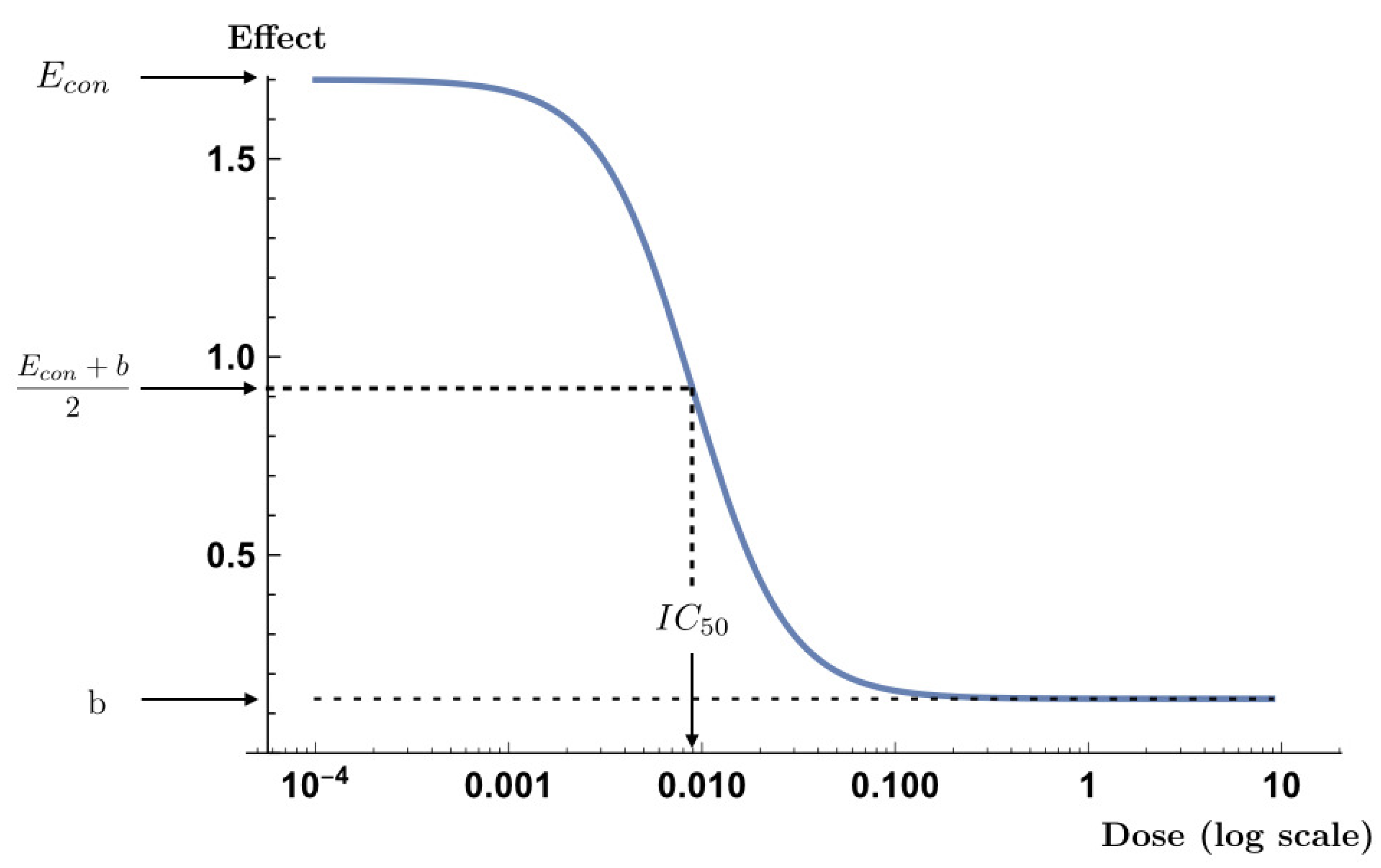
where $\mathit{\theta }=(E_{con},b,I{C}_{50},s)$ are the parameters to be estimated. The parameter $E_{con}$ is the effect on the control, i.e., where there is no dose. The parameter b corresponds to the asymptotic value of the response when the concentration of the drug tends to infinity and $I{C}_{50}$ corresponds to the dose at which a response would be found equal to the middle of the effect range, $E_{con}-b$. Finally, the parameter s is a form parameter: if $s>0$, $\eta (x;\mathit{\theta })$ will be strictly increasing, and if $s<0$, strictly decreasing. Thus, when the parameter $b>0$ and $s<0$ the drug has an inhibitory effect where b implies that the whole cell population is not destroyed, as shown in Figure 1. This is the case considered in this paper. Here it is studied from two perspectives simultaneously, where the gamma, or Poisson, is the true distribution of the response variable and the practitioner assumes a heteroscedastic normal distribution with the variance structure given by (5).

Ref. [13] bring together different maximum likelihood estimations of the parameters of (12) for different types of drugs.

Table 4. Locally D-optimal designs $\{x_1=0,x_2,x_3,x_4=D_{max}\}$ equally weighted for the 4-parameter Hill model for different drugs and probability distributions. The nominal values $E_{con}^{\left(0\right)}=1.70$ and $b^{\left(0\right)}=0.137$ were considered for all the drugs. Columns 2–4 show the nominal values of the parameters and columns 5–10 show the internal points of the D-optimal designs ${\xi }_{\mathcal{N}}$, ${\xi }_{\Gamma }$ and ${\xi }_{\mathcal{P}}$. The last column shows the efficiency when comparing the design for the heteroscedastic normal distribution with $r=0.5$ to the Poisson distribution.

	Nominal Values			${\mathit{\xi }}_{\mathbf{\Gamma }}={\mathit{\xi }}_{\mathcal{N}}(\mathit{r}=1)$		${\mathit{\xi }}_{\mathcal{N}}(\mathit{r}=0.5)$		${\mathit{\xi }}_{\mathcal{P}}$
Drug	${\mathit{IC}}_{\mathbf{50}}^{\left(\mathbf{0}\right)}$	${\mathit{s}}^{\left(\mathbf{0}\right)}$	${\mathit{D}}_{\mathit{max}}$	${\mathit{x}}_{\mathbf{2}}$	${\mathit{x}}_{\mathbf{3}}$	${\mathit{x}}_{\mathbf{2}}$	${\mathit{x}}_{\mathbf{3}}$	${\mathit{x}}_{\mathbf{2}}$	${\mathit{x}}_{\mathbf{3}}$	${\mathrm{eff}}_{\mathit{D}}\left({\mathit{\xi }}_{\mathcal{N}}\right|{\mathit{\xi }}_{\mathcal{P}})$
TMTX	0.00895	−1.79	8.95	0.00918	0.03568	0.00748	0.03010	0.00407	0.01283	0.729
MTX	0.0223	−2.74	22.3	0.02265	0.05502	0.01982	0.04922	0.01330	0.02817	0.728
AG2032	0.453	−0.825	453	0.07837	0.15728	0.07057	0.14411	0.05159	0.09299	0.728
AG2034	0.0774	−3.49	77.4	0.43634	7.70106	0.28694	5.46295	0.08152	0.96714	0.743
AG2009	111	−1.03	1500	63.1061	432.616	49.5552	361.701	23.4549	156.114	0.836

shows these nominal values and the 4-point D-optimal designs obtained for different probability distributions of the response variable: ${\xi }_{\Gamma }$ (gamma distribution with constant $\alpha$), ${\xi }_{\mathcal{N}}$ (heteroscedastic normal distribution with variance structure given by (5)) and ${\xi }_{\mathcal{P}}$ (Poisson distribution). By Theorem 1, when $r=1$ in (5) ${\xi }_{\Gamma }$ and ${\xi }_{\mathcal{N}}$ coincide. However, the designs ${\xi }_{\mathcal{P}}$ and ${\xi }_{\mathcal{N}}$ with $r=0.5$ are distinct, even though both comparisons show a similar relationship between the mean and the variance. Table 4 shows only the inner points (intermediate doses) of the D-optimal designs, as the extremes of the design space $\mathcal{X}=[0,D_{max}]$ are included in all the cases studied. The maximum dosage $D_{max}$ was given by the value $1000·I{C}_{50}$, except for the drug AG2009, since the authors considered this dosage to be impractical. It can be seen that the D-optimal design leads to experimenting with three very low doses, and at the maximum dose ($D_{max}$), except for drug AG2009, where the doses are more spread out.

The last column of Table 4 shows that the efficiency computed by (11) of the D-optimal designs when a heteroscedastic normal distribution with $r=0.5$ is assumed with respect to the Poisson distribution, is around 73%, except for the drug AG2009, whose efficiency is higher. Again, in this practical case there is a considerable loss of efficiency in estimating the model parameters, with regard to misspecification in the probability distribution. All D-optimal designs in this section have been computed using the Wynn-Fedorov’s algorithm [26].

Sensitivity Analysis

The main aim of this section is to study the effect of the relationship between $\mathrm{E}\left[y\right]$ and $\mathrm{Var}\left[y\right]$, characterized by the parameter r in (5), on the efficiency. So, a sensitivity analysis of this parameter is done. Ref. [11] studies the influence of misspecification in the structure of the variance in an analysis carried out for the gamma distribution and the heteroscedastic normal distribution separately. Here, a similar study was carried out with a point of view in which a practitioner considers a heteroscedastic normal response, but the true distribution of the response is gamma, or Poisson. For both distributions, efficiencies, using (11), are computed by comparing D-optimal designs for heteroscedastic normal distribution with the D-optimal design for the true probability distribution, as a function of the values of r.

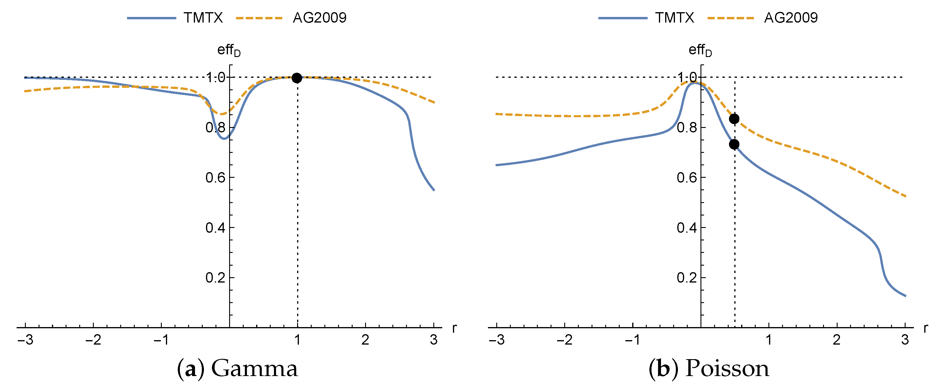
The efficiencies achieved for different drugs are shown in Figure 2. It can be seen how, when the true distribution is gamma (Figure 2a), the efficiency is 1 for $r=1$ (dot), since in this case the designs coincide as proven in Theorem 1. However, when the true distribution is the Poisson (Figure 2b), maximum efficiency is not obtained for $r=0.5$ (dots), as might be expected. It is achieved in this case for negative values of r, close to $r=0$, and so it would have been better, in terms of efficiency, for the practitioner to have assumed the homoscedastic normal distribution rather than heteroscedastic normal with $r=0.5$. Furthermore, it does not reach the value 1 for any value of r. Finally, for this model in the neighborhood of $r=0$ (homoscedastic normal distribution) opposite effects are produced on the efficiency for each of the distributions: greater efficiencies when the true distribution is the Poisson, and lower in the case of the gamma. It is important to highlight that there is no analytic explanation for this effect, and it is motivated by the model and nominal values.

For that, the effect of r on the trend of the efficiency is studied depending on the values taken by $\eta (x;\mathit{\theta })$. Again, in this analysis, it is assumed that y follows a heteroscedastic normal distribution with variance structure given by (5) when the distribution of y is the Poisson or the gamma and a misspecification takes place.

First, for sufficiently large values of r and $\eta (x;\mathit{\theta })>1$, $\forall x\in \mathcal{X}$, given that $\eta {(x;\mathit{\theta })}^{-2r}/k\approx 0$, we have

$$\begin{array}{c}\hfill {\nu }_{\mathcal{N}}(\eta (x;\mathit{\theta }),r,k)=2r^2/\eta {(x;\mathit{\theta })}^2+\eta {(x;\mathit{\theta })}^{-2r}/k\approx 2r^2/\eta {(x;\mathit{\theta })}^2\\ \hfill \propto \alpha /\eta {(x;\mathit{\theta })}^2={\nu }_{\Gamma }\left(\eta (x;\mathit{\theta })\right).\end{array}$$

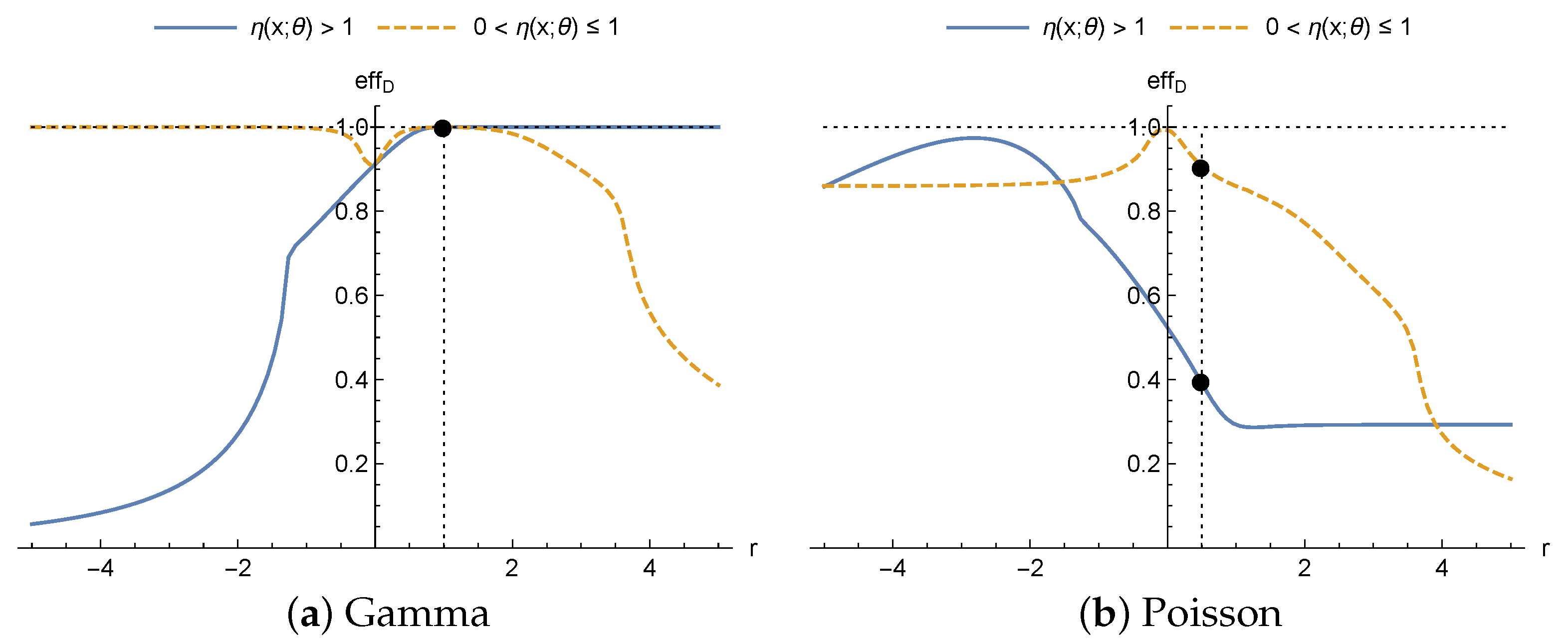
Thus, when the true probability distribution is a gamma distribution, Figure 3a (solid line) shows how, on increasing the value of r the efficiency tends to 1. On the other hand, the lower the value of r, the greater the difference between ${\nu }_{\mathcal{N}}(\eta (x;\mathit{\theta });r,k)$ and ${\nu }_{\Gamma }\left(\eta (x;\mathit{\theta })\right)$, therefore the efficiency tends to 0 as can be seen in Figure 3a. However, if $0<\eta (x;\mathit{\theta })\le 1$ (dashed line), $\forall x\in \mathcal{X}$, the effect of r on the trend of the efficiencies of the designs obtained for the heteroscedastic normal distribution when the true distribution is a gamma distribution is the opposite. As it is shown in Figure 3a, if r increases, the efficiency tends to 0, and if r decreases, the efficiency tends to 1.

When the true distribution is a Poisson distribution there is no direct comparison between its EIM and the EIM of a heteroscedastic normal distribution. However, it can be seen in Figure 3b how the efficiency reaches a maximum for a particular value of r and loses efficiency for values away from that value. This is because the study looks at values of $s<0$, and so $\eta (x;\mathit{\theta })$ and ${\nu }_{\mathcal{P}}\left(\eta (x;\mathit{\theta })\right)$ are monotonic. Therefore, the maximum efficiency is at the value of r where the distance between ${\nu }_{\mathcal{N}}\left(\eta (x;\mathit{\theta })\right)$ and ${\nu }_{\mathcal{P}}\left(\eta (x;\mathit{\theta })\right)$ is minimal (independently of whether $\eta (x;\mathit{\theta })>1$ or $0<\eta (x;\mathit{\theta })\le 1$). Although the 4-parameter Hill model is taken as an example and the graphs in Figure 3 are obtained based on that model, the whole study on the trend of r on the efficiency is general for any regression function satisfying the inequalities.

Finally, it is interesting to point out differences between the graphs in Figure 2 and Figure 3. First, the trends in the efficiencies as a function of r do not coincide. This is because, for the drugs in the study for the 4-parameter Hill model, the inequalities $\eta (x;\mathit{\theta })>1$ or $0<\eta (x;\mathit{\theta })\le 1$ are not satisfied on the design spaces considered in the examples. Secondly, when the true distribution is the Poisson distribution, maximum efficiency in Figure 3b is obtained for a value close to $r=0$ when $0<\eta (x;\mathit{\theta })\le 1$, as also it takes place in Figure 2b, while for the case with $\eta (x;\mathit{\theta })>1$ maximum efficiency is obtained close to $r=-3$, i.e., for the same model, the nominal values defined by the context of the problem affect the loss of efficiency.

6. Summary and Conclusions

This study has been carried out to analyze the effect of misspecification in the probability distribution of the response variable. We measure that effect by calculating the efficiency of the optimal design obtained with an assumed or working distribution compared to that obtained with the true probability distribution. The typical case is when a researcher assumes a normal distribution, even a heteroscedastic one, for the response variable of his or her problem, but at a greater depth, another distribution is more appropriate, for example a gamma (or Poisson) distribution. When there is misspecification in the probability distribution, there is a loss of efficiency which depends both on the assumed probability distribution and on the regression function $\eta (x;\mathit{\theta })$.

We provide some theoretical results, as well as practical ones. The first is quite general, valid for any regression function and any criterion based on FIM which guarantees that there is no loss of efficiency when the response variable follows a gamma distribution, and there is assumed to be a heteroscedastic normal distribution with $r=1$ in the variance structure given by (5). For the linear quadratic model, analytical results are obtained on computing the optimal design for Poisson and gamma distributions. These theoretical results have been used in real applications from the literature, providing designs useful for practitioners.

Finally, the 4-parameter Hill model was used to illustrate and quantify the loss of efficiency. Assuming a heteroscedastic normal distribution, taking values close to $r=0$ in (5), between about 18% and 25% efficiency is lost for all the drugs looked at in the study when the true distribution is a gamma distribution. Thus, in this case, the usual assumption of normality and homoscedasticity ($r=0$) of the response variable is not a good option. However, when the true distribution is the Poisson, the loss of efficiency is less severe, reaching maximum values of efficiency for values close to $r=0$ for all the drugs. This is a striking case, as one might expect maximum efficiency to be achieved at the value $r=0.5$, which leads to the same relationship between the mean and the variance for the heteroscedastic normal and the Poisson distributions.

It is worth finishing this paper by mentioning that the EIM is an essential tool, as it collects information both about the regression function and the probability distribution of the response variable. As already mentioned, to assume the homoscedastic normal distribution when obtaining optimal designs may lead to a great loss of efficiency. Nonetheless, the examples given show that this will depend on the true distribution of the response variable and on the model function chosen. The existence of uncertainty about the probability distribution of the response variable will therefore lead to the future goal of obtaining robust designs to reduce this uncertainty.

References

- Wang, Y.; Myers, R.H.; Smith, E.P.; Ye, K. D-optimal designs for Poisson regression models. J. Stat. Plan. Inference 2006, 136, 2831–2845. [Google Scholar] [CrossRef]
- García-Camacha, I.; Martín-Martín, R. The Construction of Locally D-Optimal Designs by Canonical Forms to an Extension for the Logistic Model. Appl. Math. 2014, 5, 824–831. [Google Scholar]
- Amo-Salas, M.; Delgado-Márquez, E.; Filová, L.; López-Fidalgo, J. Optimal designs for model discrimination and fitting for the flow particles. Stat Pap. 2016, 57, 875–891. [Google Scholar] [CrossRef]
- Aminenjad, M.; Jafari, H. Bayesian A- and D-optimal designs for gamma regression model with inverse link function. Commun. Stat. Simul. Comput. 2017, 46, 8166–8189. [Google Scholar] [CrossRef]
- Casero-Alonso, V.; López-Fidalgo, J.; Torsney, B. A computer tool for a minimax criterion in binary response and heteroscedastic simple linear regression models. Comput. Methods Programs Biomed. 2017, 138, 105–115. [Google Scholar] [CrossRef]
- Idais, O. Locally optimal designs for multivariate generalized linear models. J. Multivar. Anal. 2020, 180, 104663. [Google Scholar] [CrossRef]
- Idais, O.; Schwabe, R. Analytic solutions for locally optimal designs for gamma models having linear predictors without intercept. Metrika 2020, 86, 1–16. [Google Scholar] [CrossRef]
- Woods, D.C.; Lewis, S.M.; Eccleston, J.A.; Russell, K.G. Designs for Generalized Linear Models With Several Variables and Model Uncertainty. Technometrics 2006, 48, 284–292. [Google Scholar] [CrossRef] [Green Version]
- Stufken, J.; Yang, M. Optimal designs for generalized linear models. In Design and Analysis of Experiments, Special Design and Applications; Hinkelmann, K., Ed.; Wiley: New York, NY, USA, 2012; Chapter 4; pp. 137–164. [Google Scholar]
- Atkinson, A.C.; Fedorov, V.V.; Herzberg, A.M.; Zang, R. Elemental information matrices and optimal experimental design for generalized regression models. J. Stat. Plan. Inference 2014, 144, 81–91. [Google Scholar] [CrossRef]
- Shen, G.; Hyun, S.W.; Wong, W.K. Optimal designs based on the maximum quasi-likelihood estimator. J. Stat. Plan. Inference 2016, 178, 128–139. [Google Scholar] [CrossRef] [Green Version]
- Bezeau, M.; Endrenyi, L. Design of Experiments for the Precise Estimation of Dose-Response Parameters: The Hill Equation. J. Theor. Biol. 1986, 123, 415–430. [Google Scholar] [CrossRef]
- Khinkis, L.A.; Levasseur, L.; Faessel, H.; Greco, W.R. Optimal Design for Estimating Parameters of the 4-Parameter Hill Model. Nonlinearity Biol. Toxicol. Med. 2003, 1, 363–377. [Google Scholar] [CrossRef] [PubMed] [Green Version]
- Fang, H.B.; Ross, D.D.; Sausville, E.; Tan, M. Experimental design and interaction analysis of combination studies of drugs with log-linear dose responses. Stat. Med. 2008, 27, 3071–3083. [Google Scholar] [CrossRef]
- Sperrin, M.; Thygesen, H.; Su, T.; Harbron, C.; Whitehead, A. Experimental designs for detecting synergy and antagonism between two drugs in a pre-clinical study. Pharm. Stat. 2015, 14, 216–225. [Google Scholar] [CrossRef] [PubMed]
- McCullagh, P.; Nelder, J.A. Generalized Linear Models; Chapman & Hall/CRC: Boca Raton, FL, USA, 1989. [Google Scholar]
- Karlin, S.; Studden, W.J. Optimal Experimental Designs. Ann. Math. Stat. 1966, 37, 783–815. [Google Scholar] [CrossRef]
- Atkinson, A.; Donev, A.N.; Tobias, R.D. Optimum Experimental Designs, with SAS; Oxford University Press: New York, NY, USA, 2007; Volume 34. [Google Scholar]
- Kiefer, J.; Wolfowitz, J. The equivalence of two extremum problems. Can. J. Math. 1960, 12, 363–365. [Google Scholar] [CrossRef]
- Gaffke, N.; Idais, O.; Schwabe, R. Locally optimal designs for gamma models. J. Stat. Plan. Inference 2019, 203, 199–214. [Google Scholar] [CrossRef]
- Tucker, S.L. Tests for the fit of the linear-quadratic model to radiation isoeffect data. Int. J. Radiat. Oncol. 1984, 10, 1933–1939. [Google Scholar] [CrossRef]
- Roch-Lefèvre, S.; Martin-Bodiot, C.; Grègoire, E.; Desbrée, A.; Roy, L.; Barquinero, J.F. A mouse model of cytogenetic analysis to evaluate caesium137 radiation dose exposure and contamination level in lymphocytes. Radiat. Environ. Biophys. 2016, 55, 61–70. [Google Scholar] [CrossRef]
- McMahon, S.J. The linear quadratic model: Usage, interpretation and challenges. Phys. Med. Biol. 2019, 64, 01TR01. [Google Scholar] [CrossRef]
- Shuryak, I.; Cornforth, M.N. Accounting for overdispersion of lethal lesions in the linear quadratic model improves performance at both high and low radiation doses. Int. J. Radiat. Biol. 2021, 97, 50–59. [Google Scholar] [CrossRef] [PubMed]
- Minkin, S. Experimental Design for Clonogenic Assays in Chemotherapy. J. Am. Stat. Assoc. 1993, 88, 410–420. [Google Scholar] [CrossRef]
- Wynn, H.P. The sequential generation of D-optimum experimental designs. Ann. Math. Stat. 1970, 41, 1655–1664. [Google Scholar] [CrossRef]
Figure 1.
Graph of the regression function of the 4-parameter Hill model with nominal values corresponding to the drug TMTX, shown in Table 4.
Figure 2.
Efficiencies when comparing the designs obtained for the heteroscedastic normal distribution with variance given by (5) and different values of r when the true distributions are the gamma (a) and Poisson (b), for the 4-parameter Hill model using the nominal values of Table 4. The graphs for the drugs MTX, AG2032 and AG2034 are similar to the graph for the drug TMTX.
Figure 3.
Study of efficiency trend when comparing the designs obtained for the heteroscedastic normal distribution as a function of the parameter r of (5) considering the gamma (a) or Poisson (b) distributions as the true distributions, for the 4-parameter Hill model in . Solid lines assume and (therefore ), while for dashed lines and (). Both cases use the nominal values and .