Effective Algorithms for the Economic Lot-Sizing Problem with Bounded Inventory and Linear Fixed-Charge Cost Structure

Abstract

Efficient algorithms for the economic lot-sizing problem with storage capacity are proposed. On the one hand, for the cost structure consisting of general linear holding and ordering costs and fixed setup costs, an $\mathcal{O}\left(T^2\right)$ dynamic programming algorithm is introduced, where $T$ is the number of time periods. The new approach induces an accurate partition of the planning horizon, discarding most of the infeasible solutions. Moreover, although there are several algorithms based on dynamic programming in the literature also running in quadratic time, even considering more general cost structures and assumptions, the new solution uses a geometric technique to speed up the algorithm for a class of subproblems generated by dynamic programming, which can now be solved in linearithmic time. To be precise, the computational results show that the average occurrence percentage of this class of subproblems ranges between 13% and 45%, depending on both the total number of periods and the percentage of storage capacity availability. Furthermore, this percentage significantly increases from 13% to 35% as the capacity availability decreases. This reveals that the usage of the geometric technique is predominant under restrictive storage capacities. Specifically, when the percentage of capacity availability is below 50%, the average running times are on average 100 times faster than those when this percentage is above 50%. On the other hand, an $\mathcal{O}\left(T\right)$ on-line array searching method in Monge arrays can be used when the costs are non-speculative costs.

1. Introduction

The economic lot-sizing problem is a classical deterministic inventory problem which was independently introduced by Wagner and Whitin (abbreviated W-W) [1] and Manne [2] as an extension of the economic order quantity (EOQ) model to cases with time-varying parameters. Accordingly, the goal for this problem consists of determining an optimal procurement schedule that satisfies the demands of time for each of the $T$ time periods in which the planning horizon is divided. The cost structure defined in [1] is the sum of the fixed charge replenishment costs and the linear holding costs for each period. It is a well-known result that among the optimal solutions for the dynamic version of the EOQ, there is at least one satisfying the zero inventory ordering (ZIO) policy (i.e., an order is placed only if the inventory is depleted, which can be used to derive polynomially efficient solutions). Later, Veinott [3] proved that ZIO policies could be likewise used to derive optimal plans when the cost structure was concave in general. Since then, a significant number of contributions have been published in the literature considering diverse extensions of this simple model (refer to Brahimi et al. [4] and Wolsey [5] for more comprehensive surveys and to [6,7,8,9,10] for more recent contributions).

One of these extensions introduces bounds on the inventory levels as a consequence of the storage capacities. This version constitutes a subfamily of lot-sizing problems usually referred to as either the economic lot-sizing problem with bounded inventory (ELSPBI) or the economic lot-sizing problem with storage capacities (ELSPSC), and unfortunately, it has attracted poor attention from researchers. Throughout, the acronym ELSPBI instead of ELSPSC is used to refer to this family of problems. The importance of the ELSPBI lies primarily in its applicability in the context of material requirements planning (MRP) to improve productivity for businesses and industries. In this scenario, the decision-maker is interested in scheduling the production requirements of subassemblies (components, packaging, spare parts and raw materials involved in the manufacturing process) at the different levels within a multi-echelon system, after the firm (organization) determines or estimates the demand of finished products. Since there is normally a significant number of subassemblies involved in the manufacturing processes (e.g., automobile, pharmaceutic and aerospace industries, among others), which do not usually share the same storage area, efficient algorithms for the ELSPBI are essential to reduce the computing times needed to obtain optimal replenishment plans.

The first contribution devoted to the ELSPBI is credited to Love [11], who allowed shortages in the model and introduced a characterization of the optimal plans to derive an $\mathcal{O}\left(T^3\right)$ algorithm based on dynamic programming (the big O notation $\mathcal{O}\left(g\left(n\right)\right)$ denotes the asymtotic behavior of an algorithm, and it is used to classify them according to how their run time or space requirements grow as the input size $n$ grows. Accordingly, $f\left(n\right)=\mathcal{O}\left(g\left(n\right)\right)$ if there exist $M,n_0\in \mathbb{N}$ such that $f\left(n\right)\le Mg\left(n\right)$ for all $n\ge n_0$. Thus, $\left|f\right|$ is bounded above by $g$ (up to a constant factor) asymptotically.). Gutiérrez et al. in [12] and [13] addressed the problem, providing a new characterization and hence a new algorithm to identify optimal plans for the model with and without backorders, respectively. Even though the theoretical time complexity of the algorithm by Love could not be reduced, the computational experiment in [12] revealed that the running times were almost 30% faster than those reported by Love’s method.

In the last few decades, several time complexity improvements have been presented. For instance, Toczylowski [14] transformed the ELSPBI into an equivalent shortest-path problem in a multigraph and developed an $\mathcal{O}\left(T^2\right)$ algorithm to construct the shortest path solution. Nevertheless, even though the new approach shares the same asymptotic running time, it uses an $\mathcal{O}\left(T\log T\right)$ geometric technique inspired by the algorithm developed by Hershberger [15] to handle the class of subproblems referred to as $elementarynonsingularplans$ with $\mathrm{descending}\mathrm{edges}$, defined in [14]. Basically, a subproblem belongs to this class when its initial period is successor to a $\mathrm{breaking}\mathrm{period}$ (a period where the maximum quantity of items to be stored corresponds to the physical storage capacity in that period) and its incoming inventory level is positive.

Sedeño-Noda et al. [16] devised an $\mathcal{O}\left(T\log T\right)$ algorithm for a case without backorders or setup costs and linear ordering and holding costs. More recently, Atamtürk and Kücükyavuz [17] developed an $\mathcal{O}\left(T^2\right)$ algorithm for a case with linear and fixed holding and ordering costs and without backlogging. Their algorithm is based on the definition of a $block$, which is simply a sequence of consecutive periods satisfying certain features of the inventory levels. However, the new method computes the objective value of those blocks with a positive initial inventory level by using an $\mathcal{O}\left(T\log T\right)$ geometric method, whereas the algorithm in [17] takes $\mathcal{O}\left(T^2\right)$ time.

Taking advantage of the geometrical technique in Wagelmans et al. [18], Liu [19] and Gutiérrez et al. [20] proposed, respectively, $\mathcal{O}\left(T^2\right)$ and $\mathcal{O}\left(T\log T\right)$ algorithms assuming linear order and holding costs and setup costs, as well as backorders in the former model. Moreover, Liu [19] devised an $\mathcal{O}\left(T\right)$ method for the Wagner and Whitin (W-W) cost structure (non-speculative motives). However, Önal et al. [21] and van den Heuvel et al. [22] demonstrated independently that both the algorithm by Liu and the algorithm by Gutiérrez et al. might fail to find an optimal solution in general.

Hwang and van den Heuvel [23] addressed a general concave cost structure for procurement and holding and backlogging, and they presented a dynamic programming algorithm that runs in $\mathcal{O}\left(T^2\right)$ by using matrix-searching in a Monge array. As noted above, the algorithm proposed in this paper is also based on dynamic programming and also runs in $\mathcal{O}\left(T^2\right)$ amortized time, but it uses an $\mathcal{O}\left(T\log T\right)$ geometric method for a class of subproblems. Concretely, this class of subproblems is related to the concept of $warehousepoint$ in [23]. According to the authors, a period is said to be a warehouse point when there are inventory units available at the beginning of that period.

Most recently, Wolsey [24] derived a versatile and tight model based on a shortest path formulation that was also able to account for stock fixed costs, stock overloads and backlogging. Since the unit flow polyhedron resulting from the constraints was totally unimodular, the extreme points were binary. The author also showed that there was an $\mathcal{O}\left(T^2\right)$ algorithm that solved the problem.

The following list summarizes the most significant contributions to the ELSPBI in the literature (all of them, including the algorithm proposed in this paper, run in quadratic amortized time) along with the corresponding nomenclature of the subproblems, for which the new algorithm outperforms the existing methods. This improvement lies mainly in the use of the $\mathcal{O}\left(T\log T\right)$ geometric technique instead of using a straightforward $\mathcal{O}\left(T^2\right)$ implementation from the dynamic programming, as in those papers.

Reference	Subproblem Nomenclature
E. Toczylowski [14]	Elementary nonsingular plan
A. Atamtürk, S. Kücükyavuz [17]	Block with positive initial inventory level
H.C. Hwang, W. van den Heuvel [23]	Warehouse point

The new approach is based on what we have called $breakingperiods$ (periods when the inventory level could reach its physical storage capacity), which induces a partition of the planning horizon so that each part (subpartition) can be computed in quadratic time. However, the main contribution in this paper is that when a subpartition (subproblem) fulfils the same assumptions of either an elementary nonsingular plan as in [14] or a block as in [17] with a positive initial inventory level, or the subpartition starts with a warehouse point as in [23], the subproblem can be solved in $\mathcal{O}\left(T\log T\right)$ time by means of a geometric technique, rather than $\mathcal{O}\left(T^2\right)$ as in the previous papers. This kind of subpartition plays a relevant role in the computation of an optimal plan, since the lower the storage capacity, the greater the number of occurrences of these subproblems. Specifically, our computational experiment shows that the average occurrence percentage of this class of subproblems (i.e., the average usage rate of the geometric technique) ranges between $13\%$ and $45\%$, depending on both the total number of periods and the percentage of storage capacity availability. Furthermore, this percentage increases significantly from $13\%$ to $35\%$ as the percentage of storage capacity availability decreases. Moreover, the computational experiment also shows that when $T$ is fixed and the percentage of capacity availability is below $50\%$, the average running times are on average 100 times faster than those reported when this percentage is above $50\%$, due to the intensive use of the geometric technique. Furthermore, the new algorithm discards a large fraction of (infeasible) subproblems generated by the dynamic programming by defining upper bounds on each interval of periods.

For the case with a non-speculative cost structure, Hwang and van den Heuvel [23] claimed that the problem could be solved in $\mathcal{O}\left(T\right)$ by employing a geometric technique. However, in this paper, an on-line array-searching method in Monge arrays is proposed to obtain, in linear time, an optimal plan considering the same cost structure.

The natural extension of the single-item ELSPBI also considering the bounds on the production and replenishment quantity at each period has been addressed recently by Akbalik et al. [25]. Concretely, for the single-item CLSP-IB with a constant production capacity, time-dependent inventory bounds and concave costs, the authors showed that the problem could be solved in time $\mathcal{O}\left(T^4\right)$. They proposed an $\mathcal{O}\left(T^3\right)$ time dynamic programming algorithm for non-speculative costs.

The goal of this paper is to develop efficient algorithms for the ELSPBI with linear holding and ordering costs and set-up (fixed-charge) costs in each period. Firstly, for the general linear cost structure, the original problem is decomposed into subproblems using the notion of $\mathrm{breaking}\mathrm{periods}$. Then, some properties are introduced to effectively define recurrence equations, thereby obtaining a more precise description of the feasible set. Secondly, when the cost structure is non-speculative, it is shown that there exists an optimal plan satisfying the zero inventory ordering (ZIO) policy. Moreover, the array containing the optimal costs of all subproblems is Monge, and hence an on-line array-searching algorithm can be used to construct an optimal plan in $\mathcal{O}\left(T\right)$.

The rest of the article is organized as follows. In Section 2, the problem formulations are defined, and the procedure to decompose the original problem into subproblems is also introduced. The recurrence equations restricted to the subproblems generated by the decomposition method, as well as the procedure to implement such equations, are presented in Section 3. Furthermore, in Section 4, the dynamic programming algorithm for the ELSPBI is sketched, and a numerical example to illustrate the solution is provided. The case with the Wagner and Whitin cost structure is analyzed in Section 5. In Section 6, a computational experiment to validate the complexity and the performance of the new method is carried out. Finally, some final remarks are discussed in Section 7.

2. Problem Formulations and Breaking Periods

The ELSPBI concerns the scheduling of an optimal replenishment plan at a minimum cost that satisfies the demand in each period on time without exceeding the storage capacity. It is assumed that both the replenishment and the withdrawal of items are instantaneously completed at the beginning of each period at the warehouse.

Before formulating the ELSPBI, the following notation is introduced. Let $H=\left\{1,\dots ,T\right\}$ be the set of time periods. Throughout, let $d_t,S_t$ and $D_t={{\displaystyle \sum }}_{j=t}^T{d}_j$, $t\in H$ denote the demand and physical storage capacity in period $t$ and the cumulated demand from period $t$ to period $T$, respectively. Thus, the cumulated demand between two periods $t$ and $t^{’}$ can be easily computed as $D_{t,t’}=D_t-D_{t^{\prime }+1}$, where $D_{T+1}=0$. Moreover, the cost structure is assumed to be the sum of a setup (fixed charge) cost $f_t>0$ and linear replenishment and holding costs $p_t$ and $h_t$ through the planning horizon. Initially, no assumption is made about the speculative nature of the linear costs (i.e., it is assumed to have a general linear cost structure). The case with a non-speculative cost structure is discussed later. Additionally, the decision variables representing the order quantity in period $t$ and its corresponding binary variable are denoted by $x_t$ and $y_t$ ($y_t=0$ if $x_t=0;y_t=1$ otherwise), respectively. Likewise, the variable $I_t$ denotes the inventory level at the end of the period $t$. The list below summarizes the parameters and variables for each period $t\in H$ used to formulate the problem. Moreover, the list also provides the notation of the subproblems to be solved by dynamic programming and the data structures used in the implementation of the algorithm.

Parameters
$T$	periods of the planning horizon
$H=\left\{1,\dots ,T\right\}$	set of indices of time periods
$d_t$	demand for period $t$
$D_t={{\displaystyle \sum }}_{j=t}^T{d}_j$	cumulated demand from period $t$ to period $T$
$D_{t,t’}=D_t-D_{t^{\prime }+1}$	cumulated demand between periods $t\le t^{\prime }\in H$
$f_t$	setup (fixed charge) cost in period $t$
$p_t$	unit replenishment cost in period $t$
$h_t$	unit holding cost in period $t$
$c_t=p_t+{{\displaystyle \sum }}_{j=t}^T{h}_j$	marginal cost of ordering one unit of an item in period $t$ and holding it up to period $T$
$W_t$	maximum feasible storage usage in period $t$
$l_t$	the greatest period whose demand can be fully met from an order placed in period $t$
Variables
$x_t$	Order or replenishment quantity in period $t$
$y_t$	binary variable such that $y_t=0$ if $x_t=0;y_t=1$ otherwise
$I_t$	inventory level at the end of period $t$
$I_t^k$	inventory point (period) $k\in \left\{0,1\right\}:I_t^0=0$ and $I_t^1=W_t-d_t$
Problems
$g\left(i,j,k,l\right)$	minimum cost of the subproblem involving periods from $i$ to $j-1$ with initial and final stock levels $I_{i-1}^k$ and $I_{j-1}^l$ and where at most only one replenishment point (period) is allowed
$G\left(i,k\right)$	minimum cost of the subproblem starting in period $i$ with incoming inventory $I_{i-1}^k$ and final inventory $I_T^0=0$
Data Structures
$B$	sorted list of $\mathrm{breaking}\mathrm{periods}$ ($t\in H:W_t=S_t$) which induce a partition of the planning horizon into subpartitions (subproblems)
$Pr\left[t\right]$	array containing the number of the subproblem to which each period $t$ belongs
$F_n$	set of line segments related to the subproblem starting in (breaking) period $t_n+1$
$L_{F_n}\left(x\right)$	lower envelope of the set $F_n$ computed by an adaptation of the algorithm in [15]
${\mathcal{L}}_n$	sorted list of tuples $\left(x,t\right)$ where the first component denotes the $x$-coordinate of a breakpoint $\beta$ in $L_{F_n}$ and the second term stands for the line segment in $L_{F_n}$ containing $\beta$
$\tau \left[i,j,k,l\right]$	replenishment point (period) minimizing $g\left(i,j,k,l\right)$ (i.e., $\tau \left[i,j,k,l\right]=\mathrm{argmin}g\left(i,j,k,l\right)$)
$\mathcal{T}$	matrix containing the replenishment points (periods) $\tau \left[i,j,k,l\right]$ for all $1\le i<j\le T+1$ and $k,l\in \left\{0,1\right\}$
$succ\left[i,k\right]$	array containing two-tuples $\left(j,l\right)$ where $j$ is the inventory point (period) successor to period $i$ and $l\in \left\{0,1\right\}$ denotes the inventory level at the end of $j-1$

Accordingly, the first formulation for the ELSPBI is as follows.

$\left(\mathrm{Formulation}\mathrm{I}\right)$	$\min$	${\displaystyle {\displaystyle \sum }_{t=1}^T}\left(f_t{y}_t+p_t{x}_t+h_t{I}_t\right)$
	$s.t.$
		$I_t+d_t=x_t+I_{t-1}$	$t\in H$
		$I_{t-1}+x_t\le S_t$	$t\in H$
		$x_t-y_t{D}_t\le 0$	$t\in H$
		$I_0=I_T=0$
		$x_t,I_t\ge 0;y_t\in \left\{0,1\right\}$	$t\in H$

However, taking into account that $I_t={{\displaystyle \sum }}_{j=1}^t\left(x_j-d_j\right)={{\displaystyle \sum }}_{j=1}^t{x}_j-D_{1,t}$ for $t\in H$ and denoted by $c_t=p_t+{{\displaystyle \sum }}_{j=t}^T{h}_j$, for the marginal cost of ordering one unit of an item in period $t$ and holding it up to period $T$, the following formulation is obtained as an extension of that in [18].

$\left(\mathrm{Formulation}\mathrm{II}\right)$	$\min$	${\displaystyle {\displaystyle \sum }_{t=1}^T}\left(f_t{y}_t+c_t{x}_t\right)-{\displaystyle {\displaystyle \sum }_{t=1}^T}{h}_t{D}_{1,t}$
	$s.t.$
		${\displaystyle {\displaystyle \sum }_{t=1}^T}{x}_t=D_{1,T}$
		${\displaystyle {\displaystyle \sum }_{j=1}^t}{x}_t\ge D_{1,t}$	$t=1,\dots ,T-1$
		${\displaystyle {\displaystyle \sum }_{j=1}^t}{x}_t\le W_t+D_{1,t-1}$	$t=1,\dots ,T$
		$x_t-y_t{D}_t\le 0$	$t=1,\dots ,T$
		$x_t\ge 0;y_t\in \left\{0,1\right\}$	$t=1,\dots ,T$

The parameter $W_t$ stands for the maximum feasible storage usage in period $t$ rather than the physical storage capacity $S_t$, which can be computed as $W_t=\min \left\{W_{t+1}+d_t,S_t\right\}$, $t=T-1,\dots ,1$, with $W_T=d_T$. It is noted that $W_t-d_t\le W_{t+1}$ for all $t\in \left\{1,\dots ,T-1\right\}$ or, in general, $W_t-D_{t,t’}\le W_{t’+1}$ and $W_t-D_{t,t’}\le W_{t+1}-D_{t+1,t}$ for any $t’\ge t$. Moreover, let $l_t=\max \left\{j\in H:W_t\ge D_{t,j}\wedge W_t<D_{t,j+1}\right\}$ be the greatest period whose demand can be fully met from an order placed in period $t$. Setting $l_{T+1}=l_T=T$, the remaining values $l_t$, $t=1,\dots ,T-1$ can be determined in $\mathcal{O}\left(T\right)$ as shown below.

$\mathbf{Determining}{\mathit{l}}_{\mathit{t}}$$\mathbf{for}\mathit{t}=1,\dots ,\mathit{T}+1$$\mathbf{in}\mathcal{O}\left(\mathit{T}\right)$

$l_{T+1}=l_T=T$

$j=1$

$\mathbf{For}t=1,\dots ,T-1$ do

$\hspace{1em}\mathbf{While}{W}_t\ge D_{t,j}$$\mathrm{and}j\le T$ do

$\hspace{1em}j=j+1$

endwhile

$\hspace{1em}{l}_t=j-1$

endfor

$\mathrm{return}{l}_t$$,t\in H$

To define a dynamic programming recurrence for Formulation II, a key result to characterize optimal plans for the ELSPBI introduced by Love in [11] is used. Assuming that stockouts are not permitted, he claimed that $betweentwoadjacentinventorypoints$ (periods in which the inventory level is either 0 or at its maximum feasible capacity that can be stored) $thereisatmostoneproductionpoint$ (period with nonzero replenishment). Accordingly, let $k\in \left\{0,1\right\}$ be a superscript that indicates the value of the inventory level at the end of the inventory point $i$ so that $I_i^k=0$ if $k=0$ and $I_i^k=W_i-d_i$ if $k=1$. Moreover, let $i$ and $j$ be two consecutive inventory points, and let $g\left(i,j,k,l\right)$ denote the minimum cost of a subproblem involving periods from $i$ to $j-1$ with inventories on hand $I_{i-1}^k$ at the end of period $i-1$ and $I_{j-1}^l$ at the end of period $j-1$, respectively, and where, at most, only one replenishment point $t:i\le t\le l_i+1$ and $t<j\le l_t+1$ is allowed. Therefore, $g\left(i,j,k,l\right)$ can be expressed as follows:

$$g\left(i,j,k,l\right)=\left\{\begin{array}{ll}\underset{\begin{array}{c}i\le t\le l_i+1\\ t<j\le l_t+1\end{array}}{\min }\left(f_t\delta \left(D_{i,j-1}-I_{i-1}^k+I_{j-1}^l\right)+c_t\left(D_{i,j-1}-I_{i-1}^k+I_{j-1}^l\right)\right)\hfill & \mathrm{if}{I}_{i-1}^k\ge D_{i,t-1}\hfill \\ +\infty \hfill & \mathrm{otherwise}\hfill \end{array}\right.$$

(1)

where $\delta \left(x\right)=0$ if $x\le 0$ and $\delta \left(x\right)=1$ if $x>0$.

It is clear that a naive implementation of (1) to compute all the values $g\left(i,j,k,l\right)$ for $i\in H,j\in H\cup \left\{T+1\right\}$ and $k,l\in \left\{0,1\right\}$ takes $\mathcal{O}\left(T^3\right)$ time. This complexity actually represents a bottleneck for determining the minimum cost $G\left(i,k\right)$ of a subproblem starting in period $i$ with incoming inventory $I_{i-1}^k$ and ending in period $T+1$ with final inventory $I_T^0=0$. Note that $G\left(i,k\right)$ can be recursively expressed as

$$G\left(i,k\right)=\underset{\begin{array}{c}i<j\le l_{l_i+1}+1\\ l\in \left\{0,1\right\}\end{array}}{\min }\left(g\left(i,j,k,l\right)+G\left(j,l\right)\right)$$

(2)

where $G\left(T+1,0\right)=0$, $G\left(T+1,1\right)=+\infty$ and where $G\left(1,0\right)$ stands for the optimal cost for a corresponding instance of the ELSPBI.

At this point, the goal is to reduce the time complexity for computing (1). To this end, the values that $g\left(i,j,k,l\right)$ can take, depending on the relationship between the positions of the inventory points $i$ and $j$, are analyzed, as well as the inventory levels at these points. Accordingly, let us denote by $B=\left\{t\in H:W_t-d_t<W_{t+1}\right\}$ the sorted list of breaking periods (i.e., the set of periods $t\in H$ for which $W_t=S_t$). The term breaking periods is used to refer to the periods in $B$ because they break the monotonicity when determining the values of $W_t$, $t=1,..,T$. It is noted that, given two consecutive breaking periods $t_n<t_{n+1}$ in $B$, the sequence of values $W_{t_n+1}\ge W_{t_n+2}\ge \cdots \ge W_{t_{n+1}}$ is monotonically nonincreasing. A simple procedure to generate the sorted list $B$ and the array $Pr$ is sketched in Procedure 1, where $Pr\left[t\right]$ gives the number of the subproblem containing period $t\in H$.

Procedure 1: Construct the sorted list  $B$  and the array  $Pr$  in  $\mathcal{O}\left(T\right)$

$B=\left\{\varnothing \right\}$

$n=1$

For  $t=1,\dots ,T-1$do

$\hspace{1em}Pr\left[t\right]=n$

If$W_t<W_{t+1}+d_t$  then

Insert $$ to $B$

$n=n+1$

endif

endfor

If$W_{T-1}<W_T+d_{T-1}$  then  $Pr\left[T\right]=Pr\left[T-1\right]+1$  else  $Pr\left[T\right]=Pr\left[T-1\right]$

If  $B\ne \left\{\varnothing \right\}$  then

Insert  $0$ at the beginning of $B$

Insert $T$ at the end of $B$

endif

Return $B$ and $Pr$

The breaking periods in $B$ allow us to decompose the original problem into a set of subproblems. Thus, given two consecutive breaking periods $t_n,t_{n+1}\in B$, the subproblem $P\left(t_n+1,t_{n+1}\right)$ consists of consecutive periods $t=t_n+1,\dots ,t_{n+1}$, satisfying $W_t-D_{t,t_{n+1}-1}=W_{t_{n+1}}$. Therefore, the size of subproblem $P\left(t_n+1,t_{n+1}\right)$ is given by $T_n=t_{n+1}-\left(t_n+1\right)+1=t_{n+1}-t_n$. It should be noted that if $B=\varnothing$ for a given instance of the ELSPBI, then the instance is uncapacitated, and hence it can be solved by any of the classical methods running in $\mathcal{O}\left(T\log T\right)$ (see [18,26,27]). Henceforth, we focus our attention on the case where list $B$ is not empty. Let $\left|B\right|$ denote the number of breaking periods and, consequently, $\left|B\right|-1$ denotes the number of subproblems. Accordingly, when $B\ne \left\{\varnothing \right\}$, then $t_1=0$ and $t_{\left|B\right|}=T$.

3. Restricted Recurrence Equations

Now, some properties to reduce from $\mathcal{O}\left(T^3\right)$ to $\mathcal{O}\left(T^2\right)$ the time complexity of the solution method to compute (1) are shown. In Properties 1 and 2 below, the case to determine $g\left(i,j,k,l\right)$ when $i$ and $j$ are within the same subproblem (i.e., when $t_n+1<i<j\le t_{n+1}$) is first addressed. Under this assumption, a result similar to the planning horizon theorem, first introduced by Wagner and Whitin [1] , is provided. Afterward, the case in which $i=t_n+1,n=2,\dots ,\left|B\right|-1$ and $k=1$ is separately analyzed in Property 3, because computing $g\left(t_n+1,j,1,l\right)$ differs from the former technique for intermediate periods. Specifically, the lower envelope of the set of line segments $F_n=\left\{s_t\left(x\right)=f_t+c_{t}x|t=t_n+1,\dots ,l_{t_n}+1\mathrm{and}x\in \left(\left.0,W_t-\left(I_{t_n}^1-D_{t_n+1,t-1}\right)\right]\right.\right\}$, related to the subproblem starting in period $t_n+1$, is constructed in $\mathcal{O}\left(T_n\log T_n\right)$. Once the lower envelope $L_{F_n}\left(x\right)=\underset{t_n+1\le t\le l_{t_n}+1}{\min }{s}_t\left(x\right)$ has been constructed using, for instance, an adaptation of the classical approach described in [15] , a list ${\mathcal{L}}_n$ of tuples of the form $\left(x,t\right)$, where the first component stands for the $x$-coordinate of a breakpoint $\beta$ in $L_{F_n}$ and the second term indicates the line segment $s_t$ such that $\beta \in L_{F_n}\cap s_t$, can be defined. Note that the list ${\mathcal{L}}_n$ is sorted in increasing order of the $x$-coordinates, and we denote by ${\mathcal{L}}_n\left[m\right].x$ and ${\mathcal{L}}_n\left[m\right].t$ the $x$-coordinate and the corresponding replenishment point $t$ related to the breakpoint at position $m$ in ${\mathcal{L}}_n$, respectively. Besides that, the overall time complexity to construct all the lower envelopes $L_{F_n}\left(x\right)$ for $n=2,\dots ,\left|B\right|$-1 is

$${{\displaystyle \sum }}_{n=2}^{\left|B\right|-1}\mathcal{O}\left(T_n\log T_n\right)\le {{\displaystyle \sum }}_{n=2}^{\left|B\right|-1}\mathcal{O}\left(T_n\log T\right)\le \mathcal{O}\left(\log T\right){{\displaystyle \sum }}_{n=2}^{\left|B\right|-1}\mathcal{O}\left(T_n\right)\le \mathcal{O}\left(T\log T\right).$$

To determine $g\left(t_n+1,j,k,l\right)$, it suffices to seek for, by binary search, the consecutive values of $x$-coordinates in ${\mathcal{L}}_n$, ${\mathcal{L}}_n\left[m\right].x$ and ${\mathcal{L}}_n\left[m+1\right].x$ such that ${\mathcal{L}}_n\left[m\right].x\le D_{t_n+1,j-1}-I_{t_n}^k+I_{j-1}^l<{\mathcal{L}}_n\left[m+1\right].x$ for $j=t_n+2,\dots ,l_{t_n+1}+1$ and the corresponding line segment $s_{{\mathcal{L}}_n\left[m\right].t}$. It is noted that the case where $n=1$ does not need to be considered because $i=t_1+1=1$, and hence $g\left(1,j,1,l\right)=\infty$. Finally, the case in which the inventory points $i$ and $j$ are not in the same subproblem is discussed in Property 4.

Property 1. 

Given two consecutive breaking periods $t_n<t_{n+1}$ in $B$, the replenishment point $t$ that minimizes $g\left(i,j,k,l\right)$ is not smaller than the replenishment point $t’$ minimizing $g\left(i-1,j,k,l\right)$ when either $t_n+1<i-1<j\le t_{n+1}$ and $k,l\in \left\{0,1\right\}$ or if $k=0,l\in \left\{0,1\right\}$ and $t_n+1=i-1$.

Proof. 

Suppose that $t^{\prime }>t$. Then, the following cases can arise:

• If $k=0$ and $d_{i-1}\ne 0$, then $t^{\prime }=i-1$, and hence $t^{\prime }<t$;
• If $k=0$ and $d_{i-1}=0$, then $g\left(i-1,j,k,l\right)=\min \left(f_{i-1}+c_{i-1}\left(D_{i,j-1}+I_{j-1}^l\right),g\left(i,j,k,l\right)\right)$ because $D_{i-1,t-1}=D_{i,t-1}$ and $I_{i-2}^k=I_{i-1}^k=0$. Thus, either $t^{\prime }=i-1$ or $t^{\prime }=t$, and hence $t^{\prime }\le t$;
• If $k=1$, then $I_{i-2}^k=I_{i-1}^k+d_{i-1}=W_{i-1}$ and $I_{i-1}^k=W_{i-1}-d_{i-1}=W_i$, and hence

  $$g\left(i-1,j,k,l\right)=\min \left(f_{i-1}+c_{i-1}\left(D_{i-1,j-1}-I_{i-2}^k+I_{j-1}^l\right),g\left(i,j,k,l\right)\right)$$

  (3)

Clearly, the quantity to be replenished in period $i-1$ must be greater than $0$ (i.e., $D_{i-1,j-1}-I_{i-2}^k+I_{j-1}^l>0$) so that period $i-1$ is a replenishment period. However, $D_{i-1,j-1}+I_{j-1}^l\le I_{i-2}^k=W_{i-1}$ to ensure the feasibility of the decision, which implies that period $i-1$ is not actually a replenishment period and $g\left(i-1,j,k,l\right)=g\left(i,j,k,l\right)$, and hence $t^{\prime }=t$. It is noted that the same argument can be applied to the rest of the periods in the subproblem (i.e., for $\widehat{t}=i-1,\dots ,j$, $W_{i-1}-D_{i-1,\widehat{t}-1}=W_{\widehat{t}}$), and hence no replenishment is possible if $k=l=1$. Therefore, $g\left(i,j,k,l\right)=0$ and $t^{\prime }=t=T+1$ ($dummyperiod$). Conversely, if $k=1$ and $l=0$, then $g\left(i,j,1,0\right)=\infty$ since if $k=1$, then necessarily, $l=1$ as well.

Moreover, as Equation (3) holds for all $t_n+1<i<j\le t_{n+1}$ and $k,l\in \left\{0,1\right\}$, $g\left(i,j,k,l\right)$ can be determined applying the following result. □

Property 2. 

Given $l\in \left\{0,1\right\}$ and two consecutive breaking periods $t_n<t_{n+1}$ in $B$, the cost $g\left(i,j,k,l\right)$ for either $k\in \left\{0,1\right\}$ and $t_n+1<i<j\le t_{n+1}$ or $k=0$ and $t_n+1=i$ can be recursively determined as follows:

$$g\left(i,j,k,l\right)=\left\{\begin{array}{ll}+\infty \hfill & ifk>l,\hfill \\ 0\hfill & ifk=l=1,\hfill \\ f_i+c_i\left(D_{i,j-1}+I_{j-1}^l\right)\hfill & ifk=0and{d}_i\ne 0,\hfill \\ \min \left(f_i\delta \left(D_{i,j-1}+I_{j-1}^l\right)+c_i\left(D_{i,j-1}+I_{j-1}^l\right),g\left(i+1,j,k,l\right)\right)\hfill & ifk=0and{d}_i=0.\hfill \end{array}\right.$$

(4)

Proof. 

By virtue of the characterization described in [11], it is well known that there must be at most one replenishment point between two inventory points $i$ and $j$. Moreover, as $k$ and $l$ are given for $i$ and $j$, the inventories on hand are also fixed for all the intermediate periods $i\le t<j$, and hence the following cases can be distinguished:

• If $k=1$, $l=0$ and $i>t_n+1$, then the inventory on hand at the end of period $i-1$ is enough to satisfy the demands for periods $i$ through $j-1$ and to hold $I_{i-1}^k-D_{i,j-1}\ne 0$ units at the end of period $j-1$. Therefore, this case is infeasible for all $t_n<i<j\le t_{n+1}$ since it is assumed that $l=0$ and hence, $I_{j-1}^l=0$. Consequently, $g\left(i,j,k,l\right)=+\infty$;
• If $k=l=1$ and $i>t_n+1$, then the inventory on hand $I_{i-1}^k$ at the end of period $i-1$ is enough to satisfy the demands for periods $i$ through $j-1$ and to hold $I_{j-1}^l$ units at the end of period $j-1$. Therefore, there cannot be a replenishment point between $i$ and $j$, and $g\left(i,j,k,l\right)=0$ for all $t_n+1<i<j\le t_{n+1}$;
• If $k=0$ and $l=0$, then there must be at most one replenishment point between $i$ and $j$ whenever $D_{i,j-1}\ne 0$. Clearly, the replenishment point must be either the period $i$ or the period that minimizes $g\left(i+1,j,k,l\right)$, according to (3) in Property 1;
• If $k=0$ and $l=1$, then there must be at most one replenishment point between $i$ and $j$, even when $D_{i,j-1}=0$. Again, the replenishment point should be either the period $i$ or the period that minimizes $g\left(i+1,j,k,l\right)$, according to (3) in Property 1.

Therefore, the values $g\left(i,j,k,l\right)$ for $t_n<i<j\le t_{n+1}$ can be computed in constant time, which leads to a time complexity of $\mathcal{O}\left(T_n^2\right)$. Given that $T={\displaystyle \sum }_{n=1}^{\left|B\right|-1}{T}_n$, then the overall time complexity to compute all the values $g\left(i,j,k,l\right)$, $t_n<i<j\le t_{n+1}$ and $n=1,\dots ,\left|B\right|-1$ is $\mathcal{O}\left(T^2\right)$.

The next property addresses the case in which the inventory point $i$ is a period successor to a breaking period (i.e., $i=t_n+1$) for $n>1$, and hence, either $I_{i-1}^k=0$ or $I_{i-1}^k=S_{t_n}-d_{t_n}$ if $t_n<T$. Under this assumption, Property 1 and Property 2 are no longer applicable, because it cannot be ensured that $g\left(i,j,k,l\right)=\min \left(f_i+c_i\left(D_{i,j-1}+I_{j-1}^l-I_{i-1}^k\right),g\left(i+1,j,k,l\right)\right)$ when $k=1\left(I_{i-1}^k=I_{t_n}^1=S_{t_n}-d_{t_n}\right)$. This situation is related to the notions of an elementary nonsingular plan in [14] or a block in [17] with a positive initial inventory level, or a subproblem starting with a warehouse point as in [23], which were solved in $\mathcal{O}\left(T^2\right)$.

Note that the inventory on hand $I_{i-1}^k$ at the end of period $i-1$ is not enough to fully meet the demands for periods $i$ through $l_{t_n}+1$. Thus, an order should be placed in that period $t=\mathrm{argmin}g\left(i,j,k,l\right)$; in other words, $f_t+c_t\left(D_{i,j-1}+I_{j-1}^l-I_{i-1}^k\right)=\underset{i\le t^{\prime }\le l_{t_n}+1<j}{\min }\left(f_{t^{\prime }}+c_{t^{\prime }}\left(D_{i,j-1}+I_{j-1}^l-I_{i-1}^k\right)\right)$. Instead of using an $\mathcal{O}\left(T_n\right)$ sequential search to determine such a period, period $t$ can be obtained in $\mathcal{O}\left(\log T_n\right)$ by a binary search if the lower envelope $L_{F_n}\left(x\right)$ of the set of line segments $F_n$ on the interval $\left(\left.0,D_{t_n+1,t_{n+1}}+I_{t_{n+1}}^1\right]\right.$ was previously computed in $\mathcal{O}\left(T_n\log T_n\right)$ time. Clearly, given a period $j:i<j\le t_{n+1}$ and $l\in \left\{0,1\right\}$, if $D_{t_n+1,j-1}-I_{t_n}^k+I_{j-1}^l\notin \left(\left.0,D_{t_n+1,t_{n+1}}+I_{t_{n+1}}^1\right]\right.$, then $g\left(i,j,k,l\right)=\infty$. Conversely, either $t={\mathcal{L}}_n\left[1\right].t$ if there is only one entry in ${\mathcal{L}}_n$, or there must be two adjacent entries, say $m$ and $m+1$, in list ${\mathcal{L}}_n$ such that ${\mathcal{L}}_n\left[m\right].x\le D_{t_n+1,j-1}-I_{t_n}^1+I_{j-1}^l<{\mathcal{L}}_n\left[m+1\right].x$, and hence $t={\mathcal{L}}_n\left[m\right].t$. □

Property 3. 

Given $k=1,l\in \left\{0,1\right\}$ and $n>1$, the cost $g\left(t_n+1,j,1,l\right)$ for $t_n+1<j\le l_{t_n+1}+1$ can be determined as follows:

$$g\left(t_n+1,j,1,l\right)=\left\{\begin{array}{ll}0\hfill & if{D}_{t_n+1,j-1}+I_{j-1}^l=I_{t_n}^1,\hfill \\ f_t+c_t\left(D_{t_n+1,j-1}-I_{t_n}^1+I_{j-1}^l\right)\hfill & ift<jand{D}_{t_n+1,j-1}-I_{t_n}^1+I_{j-1}^l\in \left(\left.0,W_t-\left(I_{t_n}^1-D_{t_n+1,t-1}\right)\right]\right.\hfill \\ +\infty \hfill & otherwise\hfill \end{array}\right.,$$

(5)

where the replenishment point $t=\underset{t_n+1\le t^{\prime }\le l_{t_n}+1}{\mathrm{argmin}}\left(f_{t^{\prime }}+c_{t^{\prime }}\left(D_{t_n+1,j-1}-I_{t_n}^1+I_{j-1}^l\right)\right)$ is initially determined in $\mathcal{O}\left(\log T_n\right)$ by a binary search of the first component of the tuples in list ${\mathcal{L}}_n$. If $t\ge j$, then a sequential search is implemented to finally obtain in $\mathcal{O}\left(T_n\right)$ the actual period $t<j$ with the minimum cost.

Proof. 

Clearly, if $D_{t_n+1,j-1}+I_{j-1}^l=I_{t_n}^k$, there is no need to place an order, and $g\left(t_n+1,j,k,l\right)=0$. Let us assume now that $D_{t_n+1,j-1}-I_{t_n}^k+I_{j-1}^l\in \left(\left.0,W_t-\left(I_{t_n}^1-D_{t_n+1,t-1}\right)\right]\right.$. If ${\mathcal{L}}_n$ has only one entry, then $t={\mathcal{L}}_n\left[1\right].t$. Otherwise, there must be two consecutive entries, say $m$ and $m+1$, in ${\mathcal{L}}_n$ such that ${\mathcal{L}}_n\left[m\right].x\le D_{t_n+1,j-1}-I_{t_n}^1+I_{j-1}^l<{\mathcal{L}}_n\left[m+1\right].x$. Thus, the replenishment point $t={\mathcal{L}}_n\left[m\right].t$ is optimal for $g\left(t_n+1,j,1,l\right)$ because it is feasible (i.e., $D_{t_n+1,t-1}\le I_{t_n}^1$ ), and the cost returned by (5) is minimal because the line segment $s_t$ is either partially or completely contained in $L_{F_n}$, or $s_t$ is the feasible segment $(t<j)$ above the lower envelope with a minimum cost. On the contrary, when $D_{t_n+1,j-1}+I_{j-1}^l<I_{t_n}^k$ for some period, $j\le t_{n+1}$ is due to $k=1$ and, thereby, the inventory on hand $I_{t_n}^1=S_{t_n}-d_{t_n}$ is above the requirements to satisfy $D_{t_n+1,j-1}+I_{j-1}^l$. Consequently, an infeasibility occurs, since the actual inventory on hand at the end of period $j-1$ is greater than $I_{j-1}^l$, which leads to $g\left(t_n+1,j,k,l\right)=+\infty$. □

The case in which periods $i$ and $j$ are not in the same subproblem $P\left(t_n+1,t_{n+1}\right)$ (i.e., $t_n<i\le t_{n+1}<j$) is addressed below.

Property 4. 

Given $k,l\in \left\{0,1\right\}$, the cost $g\left(i,j,k,l\right)$ for $t_n<i\le t_{n+1}<j$ can be recursively determined as follows:

$$g\left(i,j,k,l\right)=\{\begin{array}{ll}{f}_i+c_i\left(D_{i,j-1}+I_{j-1}^l\right)& ifk=0,D_{i,j-1}+I_{j-1}^l\le W_i,d_i\ne 0,\\ \min \left(f_i\delta \left(D_{i,j-1}+I_{j-1}^l\right)+c_i\left(D_{i,j-1}+I_{j-1}^l\right),g\left(i+1,j,k,l\right)\right)& ifk=0,D_{i,j-1}+I_{j-1}^l\le W_i,d_i=0,\\ g\left(i+1,j,k,l\right)& ifk=0,D_{i,j-1}+I_{j-1}^l>W_i,d_i=0,\\ g\left(t_{n+1}+1,j,k,l\right)& ifk=1andi-1>t_n,\\ +\infty & otherwise.\end{array}$$

(6)

Proof. 

Let us analyze the following cases:

• When $k=0$ and $D_{i,j-1}+I_{j-1}^l\le W_i$, then it is feasible to place a single order to satisfy the required quantity $D_{i,j-1}+I_{j-1}^l$ as in Property 2, depending on whether $d_i\ne 0$ or $d_i=0$. When $D_{i,j-1}+I_{j-1}^l>W_i$, no replenishment can be placed in period $i$. However, if $d_i=0$, then $g\left(i,j,k,l\right)=g\left(i+1,j,k,l\right)$;
• When $k=1$, two situations may occur. On the one hand, when $i-1>t_n$, the inventory on hand $I_{i-1}^k$ at the end of period $i-1$ is enough to satisfy the demands for periods $i$ through $t_{n+1}$ and to hold $I_{t_{n+1}}^k=W_{t_{n+1}}-d_{t_{n+1}}$ units at the end of period $t_{n+1}$. Therefore, no replenishment can be placed between $i$ and $t_{n+1}$, since the inventory capacity in that period is at its maximum. The only admissible decision is to order $D_{t_{n+1}+1,j-1}+I_{j-1}^l-I_{t_{n+1}}^k$ in that period $t_{n+1}+1\le t\le l_{t_{n+1}}+1$ that minimizes the corresponding cost, and hence $g\left(i,j,k,l\right)$ reduces to calculate $g\left(t_{n+1}+1,j,k,l\right)$ using Property 3. On the other hand, if $i-1=t_n$, two replenishments must be placed to meet the quantities $\left(D_{t_n+1,t_{n+1}}+I_{t_{n+1}}^{k^{\prime }}-I_{t_n}^1\right)$ and $\left(D_{t_{n+1}+1,j-1}-I_{t_{n+1}}^{k^{\prime }}+I_{j-1}^l\right)$ with $k^{\prime }\in \left\{0,1\right\}$, and hence $g\left(i,j,k,l\right)=+\infty$. The exception in this case is when $j=t_{n+1}+1$. If this occurs, $k^{\prime }$ and $l$ must be necessarily equal, and the cost $g\left(t_n+1,t_{n+1}+1,k,l\right)$ is computed according to Equation (5) in Property 3;
• For the remaining cases, either two replenishments must be placed to satisfy the quantities $\left(D_{i,t_{n+1}}+I_{t_{n+1}}^k\right)$ and $\left(D_{t_{n+1}+1,j-1}-I_{t_{n+1}}^k+I_{j-1}^l\right)$, or the inventory on hand $I_{j-1}^l=W_{t_{n+1}}-D_{t_{n+1},j-1}$ at the end of period $j-1$ does not correspond to the actual value for that variable (i.e., $I_{j-1}^l=W_{j-1}-d_{j-1}$ ) when $l=1$. Both cases lead to infeasibilities, and hence $g\left(i,j,k,l\right)=+\infty$.

An additional array to store the replenishment point related to $g\left(i,j,k,l\right)$ is necessary. Thus, let $\mathcal{T}=\left\{\tau \left[i,j,k,l\right]\right\}$ be a $T\times \left(T+1\right)\times 2\times 2$ matrix in which each element $\tau \left[i,j,k,l\right]$ represents the replenishment point that minimizes $g\left(i,j,k,l\right)$ (i.e., $\tau \left[i,j,k,l\right]=\mathrm{argmin}g\left(i,j,k,l\right)$). It is clear that when $g\left(i,j,k,l\right)=+\infty$, then $\tau \left[i,j,k,l\right]=T+1$ to indicate that a replenishment cannot be placed between the inventory points $i$ and $j$ when the inventories on hand are $I_{i-1}^k$ and $I_{j-1}^l$, respectively. Moreover, if $k=0$ and $\left(D_{i,j-1}+I_{j-1}^l\right)=0$, then $g\left(i,j,k,l\right)=0$ in Property 2 and Property 4, and therefore the procedure sets $\tau \left[i,j,k,l\right]=T+1$ to also specify that an order cannot be placed between periods $i$ and $j$. □

The method to determine the values $g\left(i,j,k,l\right)$ and $\tau \left[i,j,k,l\right]$ for all combinations $\left(i,j,k,l\right)\in H\times H\cup \left(T+1\right)\times \left\{0,1\right\}\times \left\{0,1\right\}$ is sketched in Procedure 2. Clearly, $g\left(i,j,k,l\right)=+\infty$ for those combinations with $i\ge j$, and hence $\tau \left[i,j,k,l\right]=T+1$. Moreover, setting $l_{T+1}=T$ ensures that the index $j$ does not exceed the correct range when $l_i=T$.

Procedure 2: Determine  $g\left(i,j,k,l\right)$  and  $\tau \left[i,j,k,l\right]$  for  $1\le i<j\le T+1$  and  $k,l\in \left\{0,1\right\}$  in  $\mathcal{O}\left(T^2\right)$

apply Procedure 1 to obtain the sorted list $B$ and vector $Pr$

If $B=\left\{\varnothing \right\}$ then use the geometric technique developed by Wagelmans et al. in [18]

else

initialize $g\left(i,j,k,l\right)=+\infty$ and $\tau \left[i,j,k,l\right]=T+1$, $1\le i\le T+1$, $1\le j\le T+1$ and $k,l\in \left\{0,1\right\}$

initialize $g\left(T,T+1,k,0\right)=f_T\delta \left(d_T-I_{T-1}^k\right)+c_T\left(d_T-I_{T-1}^k\right)$ and $\tau \left[T,T+1,k,0\right]=T$, for $k\in \left\{0,1\right\}$

initialize $g\left(T,T+1,k,1\right)=g\left(T,T+1,k,0\right)$ and $\tau \left[T,T+1,k,1\right]=T$, for $k\in \left\{0,1\right\}$   compute the lists ${\mathcal{L}}_n$, $n=2,\dots ,\left|B\right|-1$ in $\mathcal{O}\left(T\log T\right)$ using an adaptation of the algorithm in [15]

For  $i=T-1,\dots ,1$  do

$n=Pr\left[i\right]$

For  $j=i+1,\dots ,l_{l_i+1}+1$  do

For  $k=0,1$do

For  $l=0,1$  do

If  $i=t_n+1$  then

If  $k=0$  then

If $j\le t_{n+1}+1$ then compute  $g\left(t_n+1,j,0,l\right)$ using (4) in Property 2

If $g\left(t_n+1,j,0,l\right)\ne +\infty$ then           $\tau \left[t_n+1,j,0,l\right]=\mathrm{argmin}g\left(t_n+1,j,0,l\right)$          endif         else          compute $g\left(t_n+1,j,0,l\right)$ using (6) in Property 4          If $g\left(t_n+1,j,0,l\right)\ne +\infty$ then            $\tau \left[t_n+1,j,0,l\right]=\mathrm{argmin}g\left(t_n+1,j,0,l\right)$          endif         endif

elseif  $i>1$  then

compute $g\left(t_n+1,j,1,l\right)$ using (5) in Property 3

If  $g\left(t_n+1,j,1,l\right)\ne +\infty$  then           $\tau \left[t_n+1,j,1,l\right]=\mathrm{argmin}g\left(t_n+1,j,1,l\right)$          endif

endif

else

If $i>t_n+1$ and $j\le t_{n+1}$ then

compute $g\left(i,j,k,l\right)$ using (4) in Property 2

If  $g\left(i,j,k,l\right)\ne +\infty$  then           $\tau \left[i,j,k,l\right]=\mathrm{argmin}g\left(i,j,k,l\right)$          endif

else

compute $g\left(i,j,k,l\right)$ using (6) in Property 4

If  $g\left(i,j,k,l\right)\ne +\infty$  then           $\tau \left[i,j,k,l\right]=\mathrm{argmin}g\left(i,j,k,l\right)$         endif

endif

endif

endfor     endfor

endfor

endfor

endif

return $g\left(i,j,k,l\right)$ and $\tau \left[i,j,k,l\right]$ for $1\le i<j\le T$ and $k,l\in \left\{0,1\right\}$

4. Solution Method and Numerical Example

Once all the values $g\left(i,j,k,l\right)$ and $\tau \left[i,j,k,l\right]$ are computed, $G\left(1,0\right)$ is solved in $\mathcal{O}\left(T^2\right)$ as shown in Algorithm 1. This algorithm assumes that $B\ne \left\{\varnothing \right\}$; otherwise, more efficient $\mathcal{O}\left(T\log T\right)$ algorithms could be used (see, for instance, [18,26,27]). A new array, $succ$, is introduced in which each element $succ\left[i,k\right]$, $1\le i\le T$, and $k\in \left\{0,1\right\}$ is a two-tuple $\left(j,l\right)$. Precisely, the first component $succ\left[i,k\right].j$ represents the inventory point $j$ adjacent to the inventory point $i$, and the second term $succ\left[i,k\right].l$ stands for the inventory level $I_{j-1}^l$ at the end of period $j-1$. This array is used in Procedure 3 to construct the optimal plan for an instance of the ELSPBI.

Algorithm 1:Determine$\mathit{G}\left(\mathbf{1},\mathbf{0}\right)$in$\mathcal{O}\left({\mathit{T}}^{\mathbf{2}}\right)$when$\mathit{B}\mathbf{\ne }\left\{\mathbf{\varnothing }\right\}$

apply Procedure 2 to compute $g\left(i,j,k,l\right)$ and $\tau \left(i,j,k,l\right)$ for $1\le i<j\le T+1$ and $k,l\in \left\{0,1\right\}$

initialize $G\left(i,k\right)=+\infty$ and $succ\left[i,k\right]=\left(0,0\right)$ for all $1\le i\le T+1$ and $k=0,1$

initialize $G\left(T+1,0\right)=0$

For$i=T,\dots ,1$do

For $j=i+1,\dots , l_{l_i+1}+1$ do

For $k=0,1$ do

For $l=0,1$ do

If $G\left(i,k\right)>g\left(i,j,k,l\right)+G\left(j,l\right)$ then

$G\left(i,k\right)=g\left(i,j,k,l\right)+G\left(j,l\right)$

$succ\left[i,k\right]=\left(j,l\right)$

endif

endfor

endfor

endfor

endfor

return $G\left(1,0\right)$

As outlined in Procedure 3, an optimal schedule $\left(x_1,x_2,\dots ,x_T\right)$ and $\left(y_1,y_2,\dots ,y_T\right)$ can be obtained in $\mathcal{O}\left(T\right)$ for a given instance of the ELSPBI.

$\mathbf{Procedure}3:\mathbf{Determine}\mathbf{an}\mathbf{optimal}\mathbf{plan}\left({\mathit{x}}_1,{\mathit{x}}_2,\dots ,{\mathit{x}}_{\mathit{T}}\right)$$\mathbf{and}\left({\mathit{y}}_1,{\mathit{y}}_2,\dots ,{\mathit{y}}_{\mathit{T}}\right)$$\mathbf{in}\mathcal{O}\left(\mathit{T}\right)$

initialize $\left(x_1,x_2,\dots ,x_T\right)$ and $\left(y_1,y_2,\dots ,y_T\right)$ to $\left(0,0,\dots ,0\right)$

$k=0$

$i=1$

While  $i<T+1$  do

$j=succ\left[i,k\right].j$

$l=succ\left[i,k\right].l$

$x\left[\tau \left[i,j,k,l\right]\right]=D_{i,j-1}+I_{j-1}^l-I_{i-1}^k$

$y\left[\tau \left[i,j,k,l\right]\right]=1$

$i=j$

$k=l$

endwhile

return $\left(x_1,x_2,\dots ,x_T\right)$ and $\left(y_1,y_2,\dots ,y_T\right)$

A simple example consisting of $T=5$ periods is solved to illustrate Algorithm 1. The parameters and preliminary values are shown in

Table 1. Input data.

	$\mathit{t}\mathbf{=}\mathbf{1}$	$\mathit{t}\mathbf{=}\mathbf{2}$	$\mathit{t}\mathbf{=}\mathbf{3}$	$\mathit{t}\mathbf{=}\mathbf{4}$	$\mathit{t}\mathbf{=}\mathbf{5}$
$d_t$	2	0	8	3	10
$f_t$	2	4	8	6	7
$c_t$	3	28	5	10	9
$S_t$	12	4	9	15	11
$W_t$	6	4	9	13	10
$l_t$	2	2	3	5	5
$Pr\left[t\right]$	1	1	2	3	3

, where it is assumed that $c_t=p_t$ and hence $h_t=0$ for $t=1,\dots ,5$. Otherwise, if $h_t\ne 0$ for some period $t$, then the quantity ${{\displaystyle \sum }}_{t=1}^T{h}_t{D}_{1,t}$ must be subtracted from the value $G\left(1,0\right)$ to obtain the actual minimum cost.

Since $B=\left\{0,2,3,5\right\}\ne \left\{\varnothing \right\}$, three subproblems, namely $P\left(1,2\right),P\left(3,3\right)$ and $P\left(4,5\right)$, are defined, and hence the values $g\left(i,j,k,l\right)$ for $1\le i<j\le 6$ and $k,l\in \left\{0,1\right\}$ can be determined according to Procedure 2. Precisely,

Table 2. Values for g(i, j, k, l), i, j ∈ H ∪ (T + 1) and k, l ∈ {0,1}.

$G_{\left(0,0\right)}^{’}=\left(\begin{array}{cccccc}\infty & 8& 8& \infty & \infty & \infty \\ \infty & \infty & 0& 48& \infty & \infty \\ \infty & \infty & \infty & 48& \infty & \infty \\ \infty & \infty & \infty & \infty & 36& 136\\ \infty & \infty & \infty & \infty & \infty & 97\\ \infty & \infty & \infty & \infty & \infty & \infty \end{array}\right)$	$G_{\left(0,1\right)}^{’}=\left(\begin{array}{cccccc}\infty & 20& 20& \infty & \infty & \infty \\ \infty & \infty & 116& 53& \infty & \infty \\ \infty & \infty & \infty & 53& \infty & \infty \\ \infty & \infty & \infty & \infty & 136& 136\\ \infty & \infty & \infty & \infty & \infty & 97\\ \infty & \infty & \infty & \infty & \infty & \infty \end{array}\right)$
Case a. (k, l) = (0, 0)	Case b. (k, l) = (0, 1)
$G_{\left(1,0\right)}^{’}=\left(\begin{array}{cccccc}\infty & \infty & \infty & \infty & \infty & \infty \\ \infty & \infty & \infty & 28& \infty & \infty \\ \infty & \infty & \infty & 28& \infty & \infty \\ \infty & \infty & \infty & \infty & 26& 126\\ \infty & \infty & \infty & \infty & \infty & 0\\ \infty & \infty & \infty & \infty & \infty & \infty \end{array}\right)$	$G_{\left(1,1\right)}^{’}=\left(\begin{array}{cccccc}\infty & \infty & \infty & \infty & \infty & \infty \\ \infty & \infty & \infty & 33& \infty & \infty \\ \infty & \infty & \infty & 33& \infty & \infty \\ \infty & \infty & \infty & \infty & 126& 126\\ \infty & \infty & \infty & \infty & \infty & 0\\ \infty & \infty & \infty & \infty & \infty & \infty \end{array}\right)$
Case c. (k, l) = (1, 0)	Case d. (k, l) = (1, 1)

shows four $\left(T+1\right)\times \left(T+1\right)$ arrays $G_{\left(k,l\right)}^{’}=\left\{g_{i,j}^{’}=g\left(i,j,k,l\right)\right\}$, one for each combination of $\left(k,l\right)\in \left\{\left(0,0\right),\left(0,1\right),\left(1,0\right),\left(1,1\right)\right\}$, in which the element occupying row $i$ and column $j$ corresponds to the cost $g\left(i,j,k,l\right)$.

Additionally, the $T\times \left(T+1\right)$ arrays ${\mathcal{T}}_{\left(k,l\right)}=\left\{{\tau }_{ij}=\tau \left(i,j,k,l\right)\right\}$ corresponding to each combination $\left(k,l\right)$ are shown in

Table 3. Values for τ(i, j, k, l), i ∈ H, j ∈ H ∪ (T + 1) and k, l ∈ {0,1}.

${\mathcal{T}}_{\left(0,0\right)}=\left(\begin{array}{cccccc}6& 1& 1& 6& 6& 6\\ 6& 6& 6& 3& 6& 6\\ 6& 6& 6& 3& 6& 6\\ 6& 6& 6& 6& 4& 4\\ 6& 6& 6& 6& 6& 5\end{array}\right)$	${\mathcal{T}}_{\left(0,1\right)}=\left(\begin{array}{cccccc}6& 1& 1& 6& 6& 6\\ 6& 6& 2& 3& 6& 6\\ 6& 6& 6& 3& 6& 6\\ 6& 6& 6& 6& 4& 4\\ 6& 6& 6& 6& 6& 5\end{array}\right)$
Case a. (k, l) = (0, 0)	Case b. (k, l) = (0, 1)
${\mathcal{T}}_{\left(1,0\right)}=\left(\begin{array}{cccccc}6& 6& 6& 6& 6& 6\\ 6& 6& 6& 3& 6& 6\\ 6& 6& 6& 3& 6& 6\\ 6& 6& 6& 6& 4& 4\\ 6& 6& 6& 6& 6& 6\end{array}\right)$	${\mathcal{T}}_{\left(1,1\right)}=\left(\begin{array}{cccccc}6& 6& 6& 6& 6& 6\\ 6& 6& 6& 3& 6& 6\\ 6& 6& 6& 3& 6& 6\\ 6& 6& 6& 6& 4& 4\\ 6& 6& 6& 6& 6& 6\end{array}\right)$
Case c. (k, l) = (1, 0)	Case d. (k, l) = (1, 1)

.

A $\left(T+1\right)\times 2$ array $G=\left\{G\left(i,k\right)\right\}$ is used now to store the minimum cost of the problems starting in period $i$, where $1\le i\le T$, and ending in period $T+1$, with the inventory on hand being $I_{i-1}^k$, $k\in \left\{0,1\right\}$. The arrays $G$ and $succ\left[i,k\right]$ are shown in

Table 4. Arrays G and succ for the instance in Table 1.

$G=\left(\begin{array}{cc}176& \infty \\ 176& 156\\ 176& 156\\ 133& 123\\ 97& 0\\ 0& \infty \end{array}\right)$

$succ=\left(\begin{array}{cc}\left(2,1\right)& \left(0,0\right)\\ \left(3,0\right)& \left(4,1\right)\\ \left(4,1\right)& \left(4,1\right)\\ \left(5,0\right)& \left(5,0\right)\\ \left(6,0\right)& \left(6,0\right)\\ \left(0,0\right)& \left(0,0\right)\end{array}\right)$

.

Procedure 3 leads to the optimal plan $\left(x_1=6,x_2=0,x_3=5,x_4=2,x_5=10\right)$ and $\left(y_1=1,y_2=0,y_3=1,y_4=1,y_5=1\right)$ with a minimum cost of 176.

Observe that the optimal plan ordered six units in period 1, which did not correspond to the sum of demands or to the physical capacity of the warehouse, but to the maximum feasible storage usage ($W_1$). The same occurred in period 3, where the sum of the inventory on hand ($I_2=4$ units) plus the order quantity ($x_3=5$ units) equaled $W_3=9$. However, the quantity ordered in period 4 ($x_4=2$ units) was such that when it was added to the inventory on hand ($I_3=1$ units), it just satisfied the demand in that period ($d_4=3$ units). Finally, the order quantity in period 5 met the demand for that period ($d_5=W_5=10$ units). It is worth noting that the maximum feasible storage usage ($W_t$) and not the physical storage capacity ($S_t$) was the parameter that was involved in computing an optimal solution.

5. The Wagner and Whitin Cost Structure

The cost structure proposed by Wagner and Whitin (W-W) in [1] assumes that the replenishment costs are constant (i.e., $p_t=p\ge 0$) and the holding costs are nonnegative (i.e., $h_t\ge 0$, $t=1,\dots ,T$). Accordingly, the marginal costs $c_t=p_t+{{\displaystyle \sum }}_{t^{\prime }=t}^T{h}_{t^{\prime }}$ satisfy the inequality $c_t\ge c_{t+1}$ for $t=1,\dots ,T-1$. This cost structure is also referred to as nonspeculative costs, because advancing partial orders to meet future demands does not lead to less costly solutions.

Although this case has been previously studied in [23], where the authors devised an $\mathcal{O}\left(T\right)$ algorithm inspired by the geometric technique introduced in [18], an alternative approach based on the on-line array-searching $\mathcal{O}\left(T\right)$ method in Monge arrays described in [28], is proposed. To this end, the following properties are introduced.

Property 5. 

If a Wagner and Whitin cost structure is assumed, a ZIO optimal plan for the ELSPBI can be determined.

Proof. 

For a contradiction, let us assume an optimal plan for the ELSPBI with Wagner and Whitin costs, where there are at least two consecutive replenishment points $t<t^{\prime }$ such that $I_{t^{\prime }-1}>0$. Clearly, either a better plan or an equally optimal plan can be derived by simply ordering $I_{t^{\prime }-1}$ units in period $t^{\prime }$ rather than in period $t$, which leads to savings in $\left(c_t-c_{t^{\prime }}\right)I_{t^{\prime }-1}$. By applying the same argument to the rest of the adjacent non-ZIO replenishment periods, a ZIO optimal schedule is obtained. □

According to Property 5, the search of the optimal plan must be narrowed to the case where the inventories on hand for any pair of consecutive inventory points $i$ and $j$ are zero (i.e., $k=l=0$, and so $I_{i-1}^k=I_{j-1}^l=0$). Moreover, as Property 1 holds, it follows that $\tau \left(i,j,0,0\right)\le \tau \left(i+1,j,0,0\right)$ and $succ\left[i,0\right].j\le succ\left[i+1,0\right].j$. Given that $k=0$ in the optimal solution, Property 3 is not applicable. For notational convenience, let $G\left(i\right)$ be the minimum cost of the problem starting in period $i$ and ending in period $T$ when the inventory on hand at the end of period $i-1$ is zero, and let $succ\left[i\right]$ be the replenishment period successor to period $i$. It is noted that $G\left(i\right)=G\left(i,0\right)$ and $succ\left[i\right]=succ\left[i,0\right].j$, where $G\left(i,0\right)$ and $succ\left[i,0\right].j$ were defined in the previous section. Similar to Wagelmans et al. [24], the cost $G\left(i\right)$ can be formulated using the following recurrence equation:

$$G\left(i\right)=\left\{\begin{array}{ll}\underset{i<j\le succ\left[i+1\right]}{\min }\left(f_i+c_i{D}_{i,j-1}+G\left(j\right)\right)\hfill & if{d}_i>0\hfill \\ \min \left(\underset{i+1<j\le succ\left[i+1\right]}{\min }\left(f_i+c_i{D}_{i,j-1}+G\left(j\right)\right),G\left(i+1\right)\right)\hfill & if{d}_i=0\hfill \end{array}\right.,$$

where $G\left(T+1\right)=0$ and $succ\left[T+1\right]=T+1$.

To compute the current $G\left(T\right),\dots ,G\left(1\right)$ in linear time, let us consider the $T\times \left(T+1\right)$ array $A=\left\{a\left[i,j\right]\right\}$, where

$$a\left[i,j\right]=\left\{\begin{array}{ll}{f}_i+c_i{D}_{i,j-1}+G\left(j\right)\hfill & ifi<j\le l_i+1,\hfill \\ +\infty \hfill & ifi\ge jorj>l_i+1.\hfill \end{array}\right.$$

Following similar observations to those introduced by Aggarwal and Park in [26], $G\left(i\right)$ can be expressed according to the following recurrence equation for $1\le i\le T$:

$$G\left(i\right)=\left\{\begin{array}{ll}\underset{i<j\le l_i+1}{\min }a\left[i,j\right]\hfill & if{d}_i>0,\hfill \\ \min \left(\underset{i+1<j\le l_i+1}{\min }a\left[i,j\right],G\left(i+1\right)\right)\hfill & if{d}_i=0.\hfill \end{array}\right.$$

At this point, let us demonstrate that $A$ is a Monge array. Note that $A$ is a Monge array if and only if for $1\le i_1<i_2\le T$ and $1\le j_1<j_2\le T+1$, the following inequality holds:

$$a\left[i_1,j_1\right]+a\left[i_2,j_2\right]\le a\left[i_1,j_2\right]+a\left[i_2,j_1\right]$$

(7)

Property 6. 

$A$ is a Monge array.

Proof. 

Let $A^{\prime }=\left\{a^{\prime }\left[k,l\right]\right\}$ denote a $2\times 2$ subarray of $A$, and for $k,l\in \left\{1,2\right\}$, let $r_{k,l}=f_{i_k}+c_{i_k}{D}_{i_k,j_l-1}+G\left(j_l\right)<+\infty$ be a real number. Accordingly, sixteen setting types of $A^{\prime }$ may be given:

$$\begin{array}{ccccc}\left(\begin{array}{cc}{r}_{1,1}& r_{1,2}\\ r_{2,1}& r_{2,2}\end{array}\right),& \left(\begin{array}{cc}{r}_{1,1}& r_{1,2}\\ r_{2,1}& +\infty \end{array}\right),& \cdots & \left(\begin{array}{cc}+\infty & +\infty \\ +\infty & r_{2,2}\end{array}\right),& \left(\begin{array}{cc}+\infty & +\infty \\ +\infty & +\infty \end{array}\right)\end{array}$$

Note that only those subarrays $A^{\prime }$ with real numbers in the secondary diagonal might not satisfy (7). Therefore, the next four cases could be critical and thereby need to be evaluated:

1.

If $A^{\prime }=\left(\begin{array}{cc}{r}_{1,1}& r_{1,2}\\ r_{2,1}& r_{2,2}\end{array}\right)$.

Given that $c_{i_2}\le c_{i_1}$, then $c_{i_2}{D}_{j_1,j_2-1}\le c_{i_1}{D}_{j_1,j_2-1}$, and when adding $f_{i_1}+G\left(j_1\right)+f_{i_2}+G\left(j_2\right)$ to both sides of the inequality, the following holds:

$$f_{i_1}+G\left(j_1\right)+c_{i_2}{D}_{j_1,j_2-1}+f_{i_2}+G\left(j_2\right)\le f_{i_1}+G\left(j_1\right)+c_{i_1}{D}_{j_1,j_2-1}+f_{i_2}+G\left(j_2\right).$$

Moreover, as $D_{j_1,j_2-1}=D_{i_2,j_2-1}-D_{i_2,j_1-1}$ and also $D_{j_1,j_2-1}=D_{i_1,j_2-1}-D_{i_1,j_1-1}$, then

$$f_{i_1}+c_{i_1}{D}_{i_1,j_1-1}+G\left(j_1\right)+f_{i_2}+c_{i_2}{D}_{i_2,j_2-1}+G\left(j_2\right)\le f_{i_1}+c_{i_1}{D}_{i_1,j_2-1}+G\left(j_2\right)+f_{i_2}+c_{i_2}{D}_{i_2,j_1-1}+G\left(j_1\right),$$

and hence $r_{1,1}+r_{2,2}\le r_{1,2}+r_{2,1}$ so that $A^{\prime }$ holds (7);

2.

When $A^{\prime }=\left(\begin{array}{cc}{r}_{1,1}& r_{1,2}\\ r_{2,1}& +\infty \end{array}\right)$.

This combination of values for $a^{\prime }\left[2,2\right]=+\infty$ and $a^{\prime }\left[2,1\right]=r_{2,1}<+\infty$ can only occur when $j_2>l_{i_2}+1$. However, if $j_2>l_{i_2}+1$, then $j_2>l_{i_2}+1\ge l_{i_1}+1$ since $i_1<i_2$, which leads to $a^{\prime }\left[1,2\right]=+\infty$. Therefore, the resulting subarray is a Monge array;

3.

If $A^{\prime }=\left(\begin{array}{cc}+\infty & r_{1,2}\\ r_{2,1}& r_{2,2}\end{array}\right)$.

Once again, the combination of values for $a^{\prime }\left[1,1\right]=+\infty$ and $a^{\prime }\left[2,1\right]=r_{2,1}<+\infty$ implies that $j_1>l_{i_1}+1$, which leads to $j_2>j_1>l_{i_1}+1$, and hence $a^{\prime }\left[1,2\right]=+\infty$. Thus, the resulting subarray satisfies (7);

4.

When $A^{\prime }=\left(\begin{array}{cc}+\infty & r_{1,2}\\ r_{2,1}& +\infty \end{array}\right)$.

Following identical arguments to those in the preceding points, it holds that the resulting subarray is a Monge array.

Given that all the critical cases for $A^{\prime }$ are either Monge or reduced to Monge subarrays, then $A$ is also a Monge array.

Analogous to [26], the Eppstein’s on-line array-searching algorithm in [28] can be applied to determine an optimal plan for the ELSPBI with a W-W cost structure in $\mathcal{O}\left(T\right)$ time, since $G\left(i\right)$ can be computed in constant time from $G\left(i+1\right)$ and the $i$th column minimum of $A$, and $a\left[i,j\right]$ can be also obtained from $G\left(i\right)$ in constant time for all $1\le i\le T$ and $1\le j\le T+1$. □

6. Computational Experiment

In order to validate both the time complexity and the performance of Algorithm 1, a computational experiment was carried out using C++ (g++ 5.1) and CPLEX on a MacBook Pro with an Intel Core i5 at 2.3 GHz and 8 GB of RAM running OS X Yosemite.

For each period $T$ from 10 to 100, with a step of 10, ten instances were randomly generated for each problem, with demands, setup costs and production costs uniformly distributed in the interval $\left[0,10\right]$. Moreover, the holding costs were set to $0$ in all cases, and $A\in \left\{5,10,20,25,50,100\right\}$ denotes the percentage of capacity availability. Thus, if $A=20$ for one instance, this means that the warehouse allowed an extra capacity of $20\%$ of the accumulated demand up to period $T$. Therefore, the physical storage capacity in period $t$, $S_t$, was uniformly distributed in the interval $\left[d_t,d_t+\frac{A}{100}{D}_{t+1}\right]$ to ensure the feasibility of the instances.

The output data reported by CPLEX and Algorithm 1 are shown in

Table 5. Output data of the computational experiment.

$\mathit{T}$	$\mathit{A}$	CPLEX	ALG 1	$\mathit{\beta }$	$\mathit{P}\mathit{r}\mathit{o}\mathit{p}. 3$	$\mathit{T}$	$\mathit{A}$	CPLEX	ALG 1	$\mathit{\beta }$	$\mathit{P}\mathit{r}\mathit{o}\mathit{p}. 3$
10	5	0.00299	0.00015	11.3	0.43158	60	5	0.11656	0.00247	51.6	0.40626
	10	0.00320	0.00016	11.0	0.43085		10	0.17744	0.00278	44.5	0.34104
	20	0.01891	0.00016	10.5	0.37831		20	0.17122	0.00234	35.3	0.25744
	25	0.02099	0.00016	10.3	0.38940		25	0.27469	0.00283	33.7	0.24487
	50	0.01416	0.00016	9.1	0.27863		50	0.19270	0.00308	25.4	0.17087
	100	0.04529	0.00014	7.3	0.21151		100	0.09676	0.00274	19.5	0.11570
20	5	0.00762	0.00044	19.6	0.42551	70	5	0.21274	0.00436	58.2	0.39074
	10	0.04129	0.00047	19.4	0.41511		10	0.34147	0.00407	48.7	0.32003
	20	0.03216	0.00038	18.2	0.37849		20	0.17300	0.00436	37.9	0.23139
	25	0.05471	0.00038	17.2	0.34397		25	0.29032	0.00432	37.1	0.22554
	50	0.04583	0.00038	14.2	0.27908		50	0.21935	0.00447	26.0	0.14902
	100	0.04606	0.00035	10.5	0.17480		100	0.12861	0.00408	20.0	0.10927
30	5	0.02520	0.00064	29.3	0.44306	80	5	0.24428	0.00525	63.0	0.37283
	10	0.05722	0.00085	26.0	0.37833		10	0.25894	0.00488	53.1	0.30406
	20	0.06357	0.00076	23.0	0.32821		20	0.40658	0.00454	43.0	0.23567
	25	0.12000	0.00062	22.0	0.31140		25	0.33478	0.00461	39.5	0.21222
	50	0.08627	0.00087	16.2	0.20420		50	0.22652	0.00491	30.4	0.15197
	100	0.07567	0.00071	13.3	0.16098		100	0.22512	0.00526	22.3	0.11115
40	5	0.05712	0.00152	36.4	0.41755	90	5	0.26251	0.00673	69.0	0.36266
	10	0.11096	0.00151	33.4	0.37898		10	0.38952	0.00618	56.7	0.28845
	20	0.16717	0.00142	27.9	0.29700		20	0.28925	0.00511	44.8	0.21447
	25	0.07575	0.00136	24.6	0.27455		25	0.24529	0.00614	42.3	0.20008
	50	0.07852	0.00121	20.1	0.20402		50	0.15298	0.00535	30.5	0.13162
	100	0.09048	0.00151	13.9	0.12192		100	0.14102	0.00661	22.9	0.09540
50	5	0.09562	0.00213	42.9	0.39505	100	5	0.49571	0.00766	73.4	0.35169
	10	0.11130	0.00217	37.0	0.33252		10	0.42649	0.00751	60.1	0.26814
	20	0.14278	0.00223	31.5	0.27841		20	0.39862	0.00743	47.8	0.21000
	25	0.22647	0.00221	30.1	0.25846		25	0.28704	0.00729	44.0	0.19311
	50	0.16692	0.00227	21.7	0.17446		50	0.15190	0.00706	32.3	0.13127
	100	0.10691	0.00206	17.5	0.12979		100	0.15214	0.00865	23.0	0.08664

. Specifically, columns one and seven indicate the number of periods ($T$), whereas columns two and eight show the percentage of capacity availability ($A$). The third and fourth columns, as well as columns nine and ten, provide the average running times (in seconds) of the ten instances for a fixed $T$ reported by CPLEX and Algorithm 1, respectively. Finally, the fifth and sixth columns, and similarly the eleventh and twelfth columns, list the average number of breaking periods ($\beta$) and the average usage rate of Property 3 ($Prop.3$), respectively. Specifically, the $Prop.3$ columns show the average rate of the number of calls to Property 3 (i.e., the usage of the geometric technique), which is defined as the quotient between the number of calls to Property 3 and the total number of calls to all the properties (i.e., $Prop.3/{{\displaystyle \sum }}_{i=2}^{4}Prop.i$) in Procedure 2.

As expected, the running times in Table 5 reported by Algorithm 1 were practically negligible when compared with those obtained by CPLEX. Furthermore, for a fixed $T$, the average running times provided by Algorithm 1 were almost constant, and the average number of breaking periods in $B$ diminished as parameter $A$ increased. Note that the values in the column labeled $\beta$ might have been greater than $T$ due to periods $0$ and $T$ being included in $B$. Moreover, the column $Prop.3$ in Table 5 suggests that the average rate of the number of calls to Property 3 decreased as the percentage of capacity availability increased. Conversely, this rate increased to vary within the interval $\left(35\%,45\%\right)$ in the most extreme conditions; that is when the percentage of storage capacity availability ($A$) decreased to $5\%$. The latter shows that the $\mathcal{O}\left(T\log T\right)$ geometric technique used in this paper played a decisive role in the resolution of the ELSPBI when the storage capacity availability was limiting, since it outperformed the $\mathcal{O}\left(T^2\right)$ approaches previously proposed in the literature for the same family of subproblems.

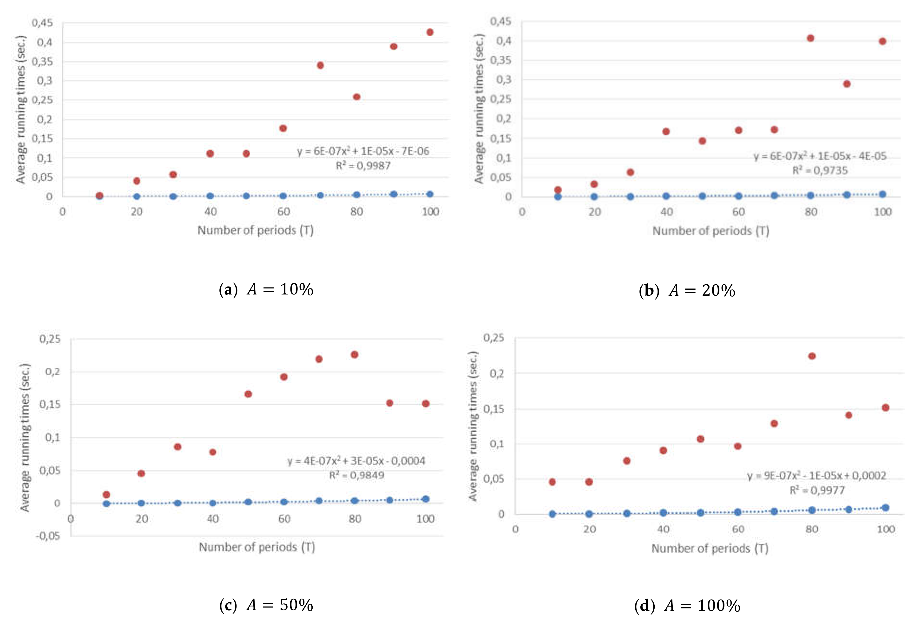
A comparison of the average running times reported by both CPLEX (in red) and Algorithm 1 (in blue) for different values of $A$ is shown in Figure 1, as well as the expression of the best fit curve for the computing times of Algorithm 1 and the coefficient of determination ($R$ square), which was above $97\%$ in all the cases. It is worth noting that when $A$ was below $50\%$, the average running times were on average 100 times faster than those reported when $A$ was above $50\%$ as a result of applying Property 3 (the geometric technique).

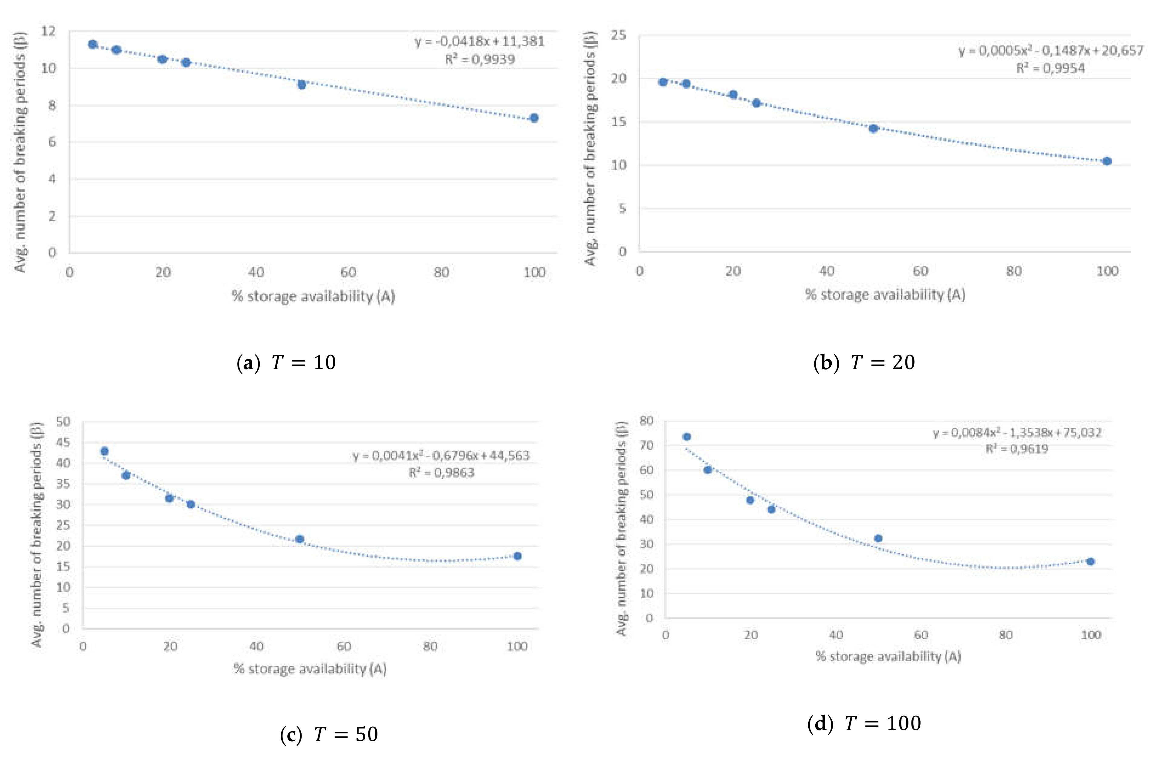
Furthermore, the average number of breaking periods in $B$ versus the parameter $A$ for different values of $T$ is depicted in Figure 2. As one would expect, the average number of breaking periods $\left(\beta \right)$ tended to diminish with the increasing percentage of capacity availability, as the empirical results in both Table 5 and Figure 2 reveal. According to the same results, the linear relationship between both parameters for relatively small values of $T$ became a quadratic curve as $T$ increased.

7. Concluding Remarks

Two dynamic programming algorithms for the ELSPBI were presented. For the general linear cost structure, the new $\mathcal{O}\left(T^2\right)$ approach focused on the evaluation of the feasible solution set by conveniently decomposing the original problem into subproblems. As the computational experiment revealed, the average number of such subproblems diminished as the storage capacity per period increased. Moreover, an $\mathcal{O}\left(T\log T\right)$ geometric technique was used to speed up the algorithm for those subproblems, fulfilling the same assumptions of either an elementary nonsingular plan as in [14] or a block with a positive initial inventory level as in [17], or the subpartition started with a warehouse point as in [23]. The computational results also showed that the usage of this technique was predominant under restrictive storage capacities, and hence when the percentage of capacity availability was below $50\%$, the average running times were on average 100 times faster than those reported when this percentage was above $50\%$.

On the other hand, for the case with non-speculative costs, we showed that an $\mathcal{O}\left(T\right)$ on-line array-searching method in Monge arrays could be used.

Clearly, the proposed algorithm cannot be used for a concave cost structure, and the method in [23] should be applied instead, even when an efficient algorithm for optimal piecewise linear function approximation is available, because its time complexity would likely be worse than $\mathcal{O}\left(T^2\right)$. However, the case where the stockouts are assumed to be backlogged (when the demand in a period cannot be met on time and it is met with an order placed in a later period) can be analyzed in future research to deal with issues (e.g., vacations or strikes) which can imply a disruption in the production process. Therefore, it should be demonstrated that the geometric technique used in this paper is also valid when the demands can be backlogged.

Another even more interesting topic is to determine whether an $\mathcal{O}\left(T\log T\right)$ algorithm can be devised for the ELSPBI with either a general concave or linear and fixed-charge cost structure. Although several researchers have focused their interest on this topic in the last few decades, this is currently a challenging open problem which likely will be overcome using some technique derived from the computational geometry.