Combined Games with Randomly Delayed Beginnings

Abstract

This paper presents two-person games involving optimal stopping. As far as we are aware, the type of problems we study are new. We confine our interest to such games in discrete time. Two players are to chose, with randomised choice-priority, between two games $G_1$ and $G_2$. Each game consists of two parts with well-defined targets. Each part consists of a sequence of random variables which determines when the decisive part of the game will begin. In each game, the horizon is bounded, and if the two parts are not finished within the horizon, the game is lost by definition. Otherwise the decisive part begins, on which each player is entitled to apply their or her strategy to reach the second target. If only one player achieves the two targets, this player is the winner. If both win or both lose, the outcome is seen as “deuce”. We motivate the interest of such problems in the context of real-world problems. A few representative problems are solved in detail. The main objective of this article is to serve as a preliminary manual to guide through possible approaches and to discuss under which circumstances we can obtain solutions, or approximate solutions.

1. Introduction

Two players are to chose, with randomised choice-priority, between two well-defined games $G_1$ and $G_2$. Priority of choice is decided by a flip of a fair coin, say, and the other player plays the alternative game. Each game $G_1$ and $G_2$ consists of two parts, a first so-called initial part, and a second one which we call the decisive part. After the choice of the games, the players have no influence on their initial parts which determine by well-defined stopping times when the decisive parts begin. Actions must be taken in the respective decisive parts only.

There are clearly many ways in which we can conceive such games, and we will confine our interest to a selection of games which seem interesting to us. Being more restrictive gives us the possibility to discuss examples in sufficient depth. We concentrate on games which are of the following form:

(i)

The initial part (called phase 1) of each game $G_1$ and $G_2$ consists of a finite sequence of independent random variables (fixed horizon). Unless stated otherwise, the laws of the random variables are known to both players.

(ii)

With ${\left({\mathcal{F}}_t^{I1}\right)}_{t\le n}$, respectively, ${\left({\mathcal{F}}_t^{I2}\right)}_{t\le n}$ denoting the filtration generated by the respective variables, we suppose that ${\tilde{\sigma }}_1$, and, ${\tilde{\sigma }}_2$ are well-defined stopping times on these initial parts. These stopping times are truncated by definition by the corresponding horizons of $G_1$ and $G_2$, say $h_1$ and $h_2$, that is we confine our interest to the stopping times ${\sigma }_1:={\tilde{\sigma }}_1\wedge h_1,{\sigma }_2:={\tilde{\sigma }}_2\wedge h_2.$

(iii)

If the event $\{{\sigma }_i=h_i\},i\in \{1,2\}$, occurs, then player i cannot enter the second decisive part of the game and loses by definition. We say then that player i fails target 1. Each player i with ${\sigma }_i<h_i$ enters the second part (phase 2) and faces a (possibly new) sequence of independent random variables. The problem is now to stop online in an optimal way on a specified event (target 2). Unless stated otherwise, both player(s) know from the beginning the targets for each game as well as the laws of the random variables.

1.1. General Situation

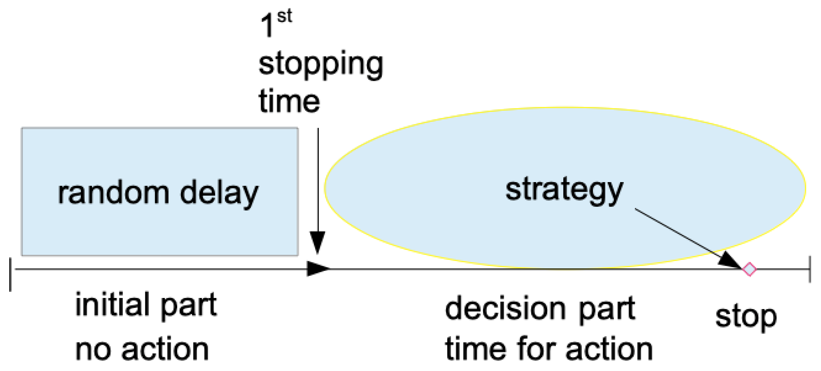
The general type of games we consider is displayed in Figure 1. Unless stated otherwise (as in Problem 4), the two players are only indirectly playing against each other, namely through the choice of their game. The games consist of two parts each, namely a phase 1 (initial part) with a specific target, and a phase 2 (strategic part) with another specific target. The player who has priority must decide which combination of the two parts is more favorable to win the combined game.

1.2. Motivation

We note that the type of games we consider in the general situation pictured in Figure 1 is a combined optimal stopping game. A priori, the game character in the usual sense of a two-person game, is missing. If we know the value $V_k$ of game $G_k,k\in \{1,2\}$, then we know which game to chose. Furthermore, after the attribution of the games to the players, the latter do not interact with each other except in Problem 4, where players may offer to switch games for a certain price. The main initial decision is to choose the game. It would make no essential difference if we formulated a corresponding problem for $r\ge 2$ games with r of players. However, for convenience and simplicity we always confine to the case $r=2.$

The general setting reflects, as we think, features we see in real world problems, as for instance in business competition. One player sees an opportunity to make money in, or with, a sequence of future events. So does his or her competitor (2nd player). However, both realise that there is not enough room for both to pursue the same goal, and thus alternatives are examined. If there is one, then it will typically be in form of another stream of events, i.e., an alternative game. Each business plan needs preparation, as things may first have to develop to fulfil a certain “pattern” (primary goal = target 1), realised at some stopping time $\sigma$ before the environment seems favorable to allow to implement the business plan. $\sigma$ is the starting point of phase 2 when the player will optimise his or her strategy. Priority in the real world is typically given by being quick rather than through a flip of coin. Furthermore, in real world both players can be winners (as in our setting), but each would typically like to choose the game with the highest promise of success.

1.3. Related Work

Although this type of problems seems to be new, there exist several studies in the literature which are related, or weakly related. Specific references will be given in the text. Sometimes the link seems weak, but the present paper tries also be a little guide to some connections. Therefore it is adequate to reference at least some of these connections, without trying to go into details.

In the present introduction section we first recall a few general sources.

A wide range of information about the variety of mathematical games and methods of solution can be found for instance in the book by Mazalov [1], or in the recent book by Ferguson [2]. For the theory of Optimal Stopping including free boundary problems we to refer to Peskir and Shiryayev [3]. For a far-going study of approximate solutions of optimal stopping problem, see Rüschendorf [4]. Although we will limit our interest to games in discrete time we also mention that Peskir found an interesting relation between the Nash equilibrium and the value function of an optimal stopping game in continuous time [5].

A closer relation with the present paper is seen in the papers by Ferenstein [6] as well as by Szajowski [7], and Szajowski [8], who study problems of optimal stopping for discrete time Markov processes. As an example, Szajowski solves a generalized best choice problem for two players. See also the review papers by Nowak and Szajowski [9] and Immorlica et al. [10].

2. Framework and Problems

To exemplify the type of games of which we are thinking, we start with an explicit example (Problem 1). This problem will be solved explicitly. We then show in how far a generalisation (Problem 2) would need a different approach to its solution, both from the theoretical and the practical side. The essentials of our approach to Problem 1 will stay valid for Problem 2, and the reader will see this without having to go through computations.

Interesting supplementary modifications of the more general setting of Problem 2 then come also naturally to our mind, and there are two of them (Problems 3 and 4) which we would like to treat in some more detail.

Problem 1.

Let $h_1$ and $h_2$ be positive integers. Two players are informed that a coin will be tossed $h=max\{h_1,h_2\}$ times. $h_i$ is what we call the horizon for game $G_i,i\in \{1,2\}.$ Tosses are supposed to be independent, each with outcome probability $\mathbf{P}\left(H\right)=p$, $\mathbf{P}\left(T\right)=q=1-p$, where $H$, respectively, $T$, stand for the events “head”, respectively, “tail”. The players know the parameter p and have the option between the following games.

• $G_1$: If the consecutive pattern $H,H,H,H$ is obtained before $h_1$ tosses, the player wants to stop online on the very last T up to toss number $h_1.$
• $G_2$: If the consecutive pattern $T,T,T,$ is obtained before $h_2$ tosses, the player wants to stop online on the very last H up to toss number $h_2.$

In the case that both players choose the same game, the priority of choice is randomised by the flip of a (fair) coin. If not specified otherwise the second player must then accept to play the remaining game. Thus, the true problem is which game the player having priority should choose. $[•]$

In Problem 1 we may see $\{H,T\}$ as an alphabet, and the h tosses as h independent draws (with replacement) from this alphabet with constant outcome probabilities $p=\mathbf{P}\left(H\right),q=\mathbf{P}\left(T\right)=1-p.$ The stopping times in phase 1 and phase 2 are determined target events. Note that, in each game, the target event of phase 1 is a pattern created by a string of length greater than 1 of elementary events, and that the second target is, in fact, also a composed event.

Problem 2.

The setting of Problem 1 is generalised as follows. Instead of coin tosses we have h independent draws from a finite alphabet $\{a_1,a_2,\cdots ,a_b\},$ and again, as in Problem 1, in each game a target event for phase 1, and another target event for phase 2. No specifications of the target events are given. This opens a whole basket of possibilities, on which we shall comment. $[•]$

Thinking of games as toy models of the real world, the player who reaches first his or her target in phase 1, has often the possibility to make the competitor withdraw from continuation. In this case, there is at most one winner.

As an example, think of an entrepreneur who, by acquiring a technological advantage, can produce certain goods cheaper than the competitor. However, then, to stay successful (phase 2), the entrepreneur must reach sufficient sales numbers of these goods (target 2). In our simplified setting, this gives rise to a third interesting problem type, exemplified by Problem 3 below.

Problem 3.

The basic setting is the same as in Problem 2 except that, if one player reaches target 1 in phase 1 strictly before the other player, then only the first one can continue and win if their or her target 2 is reached before the end of horizon. If both players reach target 1 at the same (discrete) time, both are allowed to continue. $[•]$

Note that in none of the problems we speak of rewards for winning a game. Hence, by our definition, players succeeding to get their two targets win their game. Consequently there can be two winners, or just one, or none at all, and some real-world problems may convince, that this setting has some advantages.

If, however, we want to modify this setting by attributing different (positive) rewards for winning a game, then this is no problem. We would then naturally agree to call the “real” winner the player who receives the higher reward.

As said before, we will examine the impact of possible modifications of the preceding problems, and show, or discuss, how to deal with them without solving them completely. One more natural modification merits to be understood as a problem of its own.

Problem 4.

After attributing the randomised priority, obtained by player A, say, player B either accepts to play the other game or else B offers to A an amount of money for obtaining priority. The problem is now not only which game to choose, but also what would be a fair offer for obtaining priority? Moreover, what would be a faire price for switching at an arbitrary time during a game? $[•]$

Problems 1–4 are the framework of our discussion. Problem 1 is defined in detail, and will be solved by classical methods. Problems 2 and 3 may take many different forms according to the chosen type of targets in the respective phases. We make suggestions, how to tackle the different forms. Depending on the nature of the specific targets, suggestions may turn out to be rather modest. Problem 4 is again of a different kind, and so is our Section 5 dealing with games under weak information.

2.1. Consecutive Steps to Solutions

We begin with the first step to the solution of Problem 1.

First part of the solution of Problem 1.

Since the probability of succeeding in phase 2 depends on how many draws will be available after the desired pattern in phase 1 has appeared, we compute the distribution of the first occurrence time. The latter can be obtained from a well-known renewal-type argument.

Look first at the desired pattern for $G_1.$ We denote patterns by the generic letter $\pi ,$ and the subscript will refer to the game. Hence ${\pi }_1=H,H,H,H.$ Let

$$\begin{array}{c}\hfill q_k=P\left({\pi }_1\mathrm{does}\mathrm{not}\mathrm{occur}\mathrm{up}\mathrm{to}\mathrm{k}\mathrm{th}\mathrm{toss}\right).\end{array}$$

(1)

Partitioning according to the non-occurrence of the pattern ${\pi }_1$ in the first four tosses we obtain by independence for $k\ge 4$ the recursion $q_k=\mathbf{P}\left(T\right)q_{k-1}+\mathbf{P}(H,T)q_{k-2}+\mathbf{P}(H,H,T)q_{k-3}+\mathbf{P}(H,H,H,T)q_{k-4},$ that is, with evident initial conditions $q_0=q_1=q_2=q_3=1$ and $q_4=1-p^4,$

$$\begin{array}{cc}\hfill q_k& =\sum _{j=1}^4{p}^{j-1}q{q}_{k-j},\mathrm{for}k=5,6,\cdots ,m.\hfill \end{array}$$

After having computed these $q_k$ we obtain the desired distribution, as follows. The first occurrence of ${\pi }_1=H,H,H,H$ occurs in k if ${\pi }_1$ has not appeared until step $k-5$ and will be realised at steps $k-3,k-2,k-1$ and $k.$ Note that, in order to assure that this will be the first time that the pattern ${\pi }_1$ appears up until toss $k\ge 5$, we need to see a T at step $k-4$. Hence, again by the independence of tosses, we get

$$\begin{array}{cc}\hfill {\varphi }_k& :=P\left(\mathrm{first}{\pi }_1\mathrm{at}\mathrm{k}\mathrm{th}\mathrm{toss}\right)=\left\{\begin{array}{c}0,\mathrm{if}k<4,\hfill \\ p^4,\mathrm{if}k=4,\hfill \\ q_{k-5}\mathbf{P}\left(T\right)\mathbf{P}{\left(H\right)}^4=q_{k-5}q{p}^4,\mathrm{if}k\ge 5.\hfill \end{array}\right.\hfill \end{array}$$

(2)

The value of game $G_1,$$V_1$ say, provided an optimal continuation exists, is thus just the absolute win probability under optimal play for the player playing $G_1$, that is

$$\begin{array}{cc}\hfill V_1& =\sum _{k=1}^{n-1}{\varphi }_k\mathbf{P}\left(\mathrm{optimal}\mathrm{continuation}\mathrm{after}\mathrm{k}\mathrm{stops}\mathrm{on}\mathrm{last}\mathrm{T}\right).\hfill \end{array}$$

(3)

With (1)–(3), a part of Problem 1 is solved since, passing through (1) and (2) correspondingly for the pattern ${\pi }_2=T,T,T$ we can obtain in (3) the corresponding expression for the value $V_2$ for game $G_2.$ Clearly, we can compute these values explicitly, and thus compare them, as soon as we know the optimal behaviour in both cases in phase 2 after the occurrence of the respective target pattern ${\pi }_1$ and ${\pi }_2$ of phase 1.

Intuitively, there should exist for each player in phase 2 an optimal threshold time from which onward one should stop on a tail in $G_1$, respectively, on a head in $G_2.$ This intuition turns out correct in the present example. Actually, it stays correct under more general conditions than requiring complete independence, as we shall later prove in Theorem 1. After the proof of this theorem, we will complete the solution of Problem 1.

However, we now want first to discuss the interest of such problems in more generality.

In the following we think about the true strategic part of such games, i.e., phase 2. We shall argue, that the objective of being successful is actually often an objective to obtain a so-called last success. Problem 1, where target 2 is simply a last $T$, respectively, a last H exemplifies this objective.

2.2. Last Success Problems

Last-success problems seem to attract general interest, and this independently of the context of games. One reason is that the notion of a last success is very flexible, because success can be defined as an event which is of interest for the decision maker.

So for example, in the secretary problem, we may consider each candidate who is better than all preceding ones as a record (the very first one is a record by definition). If we succeed in stopping online on the last record then we obtain the best candidate. In the same vein, if a candidate is an offer we receive for an asset we sell, stopping on the last record means selling best. Similarly we can define lower records in order to solve the problem for buying an asset for the cheapest price. See also Gnedin [11]. Among newer examples, and methods of solutions, we cite the work of Goldenshluger et al. [12] which includes several such problems in a surprisingly unified form. We also like to mention a paper with a single specific objective function, namely the paper by Grau Ribas [13]. It shows us that, for certain generalisations of a last success objective, the classical dynamic programming approach may have clear advantages.

See also Grau Ribas [14].

More should be said on flexibility. A last success need not be a record, not even be of interest itself in any sense. It may become distinguished simply by being the last one to complete a specified set. This is exemplified in a study of planning medical treatments (Bruss [15]) where a convincing way to comply with ethical constraints is to pursue a last success. Additional flexibility can also be obtained to some extent by adapting the notion of a last success to more than one selection, by focussing on the best-or-second best, as in Ano and Ando [16], Ano et al. [17], and Bayón et al. [18], looking at multiple stopping versions as in Tamaki [19] and Kurushima and Ano [20], and also by allowing for missing observations, as in the work of Ramsey [21].

Another reason for the interest in last-success problems is that the resulting optimization is often much more “robust” than one would intuitively expect, as exemplified by the $1/e$-law of Bruss [22]. The latter concerns the case of an unknown number of candidates, but this holds also for other important modifications as shown in Szajowski [23] and Ferguson (2016) as well as in the study of bounds for multiple stopping problems (Matsui and Ano [24,25]). Hence last success settings are versatile. Since we must limit our interest the general model somewhere, we propose to concentrate on these for phase 2.

3. Odds-Theorem for Delayed Stopping

In the following we need the terminology of the Odds-theorem (Bruss [26] (Th.1)) which we recall for convenience. Let $n>0$ be an integer, and let $X_1,X_2,\cdots ,X_n$ be independent Bernoulli random variables with success parameters $p_k=\mathbf{P}(X_k=1)=1-\mathbf{P}(X_k=0),k=1,2,\cdots ,n.$ The objective is to maximise the probability of stopping online on the last success, i.e., on the last $X_k=1.$ The optimal strategy to achieve this goal is obtained as follows. For $k=1,2,\cdots ,n$, let

$$\begin{array}{c}\hfill q_k=1-p_k;r_k=\frac{p_k}{q_k};Q(k,n)=\prod _{j=k}^n{q}_j;R(k,n)=\sum _{j=k}^n{r}_j,\end{array}$$

(4)

and let the integer $s\ge 1$ (called threshold index) be defined by

$$\begin{array}{c}\hfill s:=s\left(n\right)=\left\{\begin{array}{cc}1\hfill & ,\mathrm{if}R(1,n)<1\hfill \\ sup\{1\le k\le n:R(k,n)\ge 1\}\hfill & ,\mathrm{otherwise}.\hfill \end{array}\right.\end{array}$$

(5)

The strategy to stop on the first index k with $k\ge s$ and $X_k=1$, if such a k exists, maximises the probability of stopping on the last success. If no such k exists, then we have to stop at time n and lose by definition. The corresponding optimal win probability is easy to compute by the odds-algorithm (Bruss [26] (Th.1)) and equals

$$\begin{array}{c}\hfill V\left(n\right)=Q\left(s\right(n),n)R\left(s\right(n),n).\end{array}$$

(6)

3.1. Randomly Delayed Stopping

To be rigorous in our conclusions for the Problems 1–4, we need however more. Consider the case of a delay imposed by a random time W with values in $\{1,2,\cdots ,n\}.$ Stopping is not allowed before time W. As before, we want to maximise the probability of stopping on the very last success.

Does it suffice to replace simply the threshold s defined in (5) by $\tilde{s}:=max\{W,s\left(n\right)\}$ to obtain an optimal strategy? This seems trivial (and is true) if W is deterministic. In general this is not true, of course, even not true if W is a stopping time on $X_1,X_2,\cdots ,X_n$.

The following is possibly the most adequate formulation of minimum requirements needed for applying a type of an Odds-Theorem.

Theorem 1.

Let $X_1,X_2,\cdots ,X_n$ be Bernoulli random variables on a filtered probability space $(\mathrm{\Omega },\mathcal{A},\left({\mathcal{A}}_k\right),P),$ where ${\mathcal{A}}_k$ denotes the σ-field generated by $\{X_j:1\le j\le k\}.$ Suppose there exists a random time W for $X_1,X_2,\cdots ,X_n$ on the same probability space such that the $X_j$ with $j\ge W$ are independent random variables satisfying

$$\begin{array}{c}\hfill p_j\left(w\right):=\mathbf{P}(X_j=1|W\le w),1\le w\le j\le n.\end{array}$$

Then, putting $r_j\left(w\right)=p_j\left(w\right)/(1-p_j\left(w\right)),$ it is optimal to stop at the random time

$$\begin{array}{c}\hfill \tau :=inf\left\{k\in \{W,W+1,\cdots ,n\}:\{X_k=1\}\&\sum _{j=k+1}^n{r}_j\left(W\right)\le 1\right\}.\end{array}$$

(7)

Here it is understood that, if $\{·\}=\mathrm{Ø},$ we stop at time n and lose by definition.

Proof. 

Our proof will profit from the proof of the Odds-Theorem (Bruss [26]) if we rewrite the threshold index (5) in an equivalent form.

Recall the definition of $R(k,n)$ in (4).

If we define, as usual, an empty sum as zero, then s defined in (5) can be alternatively written as

$$\begin{array}{c}\hfill s^{\prime }:=s^{\prime }\left(n\right)=inf\left\{1\le k\le n:R(k+1,n):=\sum _{j=k+1}^n{r}_j\le 1\right\},\end{array}$$

(8)

which is straightforward to verify.

Recall $p_j\left(w\right)$ as defined in Theorem 1, and let for $j=w,w+1,\cdots ,n$

$$q_j\left(w\right)=1-p_j\left(w\right)=\mathbf{P}(X_j=0|W\le w).$$

This means from the assumptions concerning W that $X_w,X_{w+1},\cdots ,X_n$ are independent random variables with laws only dependent on the event $\{W\le w\}.$ If we think of w as being fixed, then we can and do define $p_j:=p_j\left(w\right)$ for all $w\le j\le n$ and use the same notation as before defined in (4) with the corresponding odds $r_j\left(w\right)=p_j\left(w\right)/q_j\left(w\right)=:r_j.$ Accordingly, we have for $k\ge w$ from (4) the simple monotonicity property $R(k,n)\ge R(k+1,n).$

It is easy to check that this monotonicity property is equivalent to the uni-modality property proved in Bruss [26] (p. 1386, lines 3–12), reference [27]. The latter implies that the optimal rule is a monotone rule in the sense that, once it is optimal to stop on a success at index $k,$ then it is also optimal to stop on a success after index $k.$ (For a convenient criterion for a stopping rule in the discrete setting being monotone, see also Ferguson [28] (p. 49)).

Note that, whatever $W=w\in \{1,2,\cdots ,n\}$, the odds $r_j:=r_j\left(w\right)$ are deterministic functions of the $p_j:=p_j\left(w\right)$, and so the future odds ${\left(r_j\right)}_{j\ge W+1}$ after the (random) time W are also known and will not change. The only restriction we have to keep in mind for the simplified notation is that the index k here satisfies $k\ge w$ on the set $\{W\le w\}.$ However, then the monotonicity property of $R(·,·)$ is also not affected, that is

$$\begin{array}{c}\hfill \forall 1\le j\le \ell :R(W+j,n)\le 1\Rightarrow R(W+\ell ,n)\le 1.\end{array}$$

Since the latter implies the uni-modality property of the resulting win probability on $\{W\le j\le n\}$, the monotone rule property is again maintained for the optimal rule after the random time $W,$ exactly as in the proof of the Odds–Theorem [26] (Th. 1, p. 1385). Therefore the optimal strategy is to stop on the first success (provided it exists) from time $\tau$ onwards where $\tau$ satisfies

$$\begin{array}{c}\hfill \tau \ge W\mathrm{and}\sum _{j=\tau +1}^n{r}_j\left(W\right)\le 1.\end{array}$$

This is the threshold index $\tau$ of Theorem 1 defined in (7) as well as the same stopping time. Hence the proof. □

Remark 1.

Note that the statement of Theorem 1 is intuitive. Its applicability may nevertheless be delicate. It depends on the $p_j$’s being predictable for all $j\ge W.$ Often this is not the case. For instance, we may have (conditionally) independent random variables, but, if we collect information about the $p_j$ from observations then the distributions of the future values of $X_{j+1},X_{j+2},\cdots$ typically depend on $X_k,1\le k\le j,$ on which the event $\{W=j\}$ may be allowed to depend!

Completing the Solution of Problem 1.

In Problem 1 we have i.i.d. draws, i.e. the conditions for Theorem 1 are clearly satisfied. Hence the optimal rule is determined by the threshold index (8). This one is here particularly simple, namely the odds $r_k$ are homogeneous in time with $r_k:=q/p$ for $G_1$, and $r_k:=p/q$ for game $G_2.$ Hence we have

$$\begin{array}{c}\hfill \mathrm{for}{G}_1:s_1\left(h_1\right)=max\left\{\ell :\sum _{j=\ell }^{h_1}\frac{q}{p}\ge 1\right\}={\left[h_1+1-\frac{p}{q}\right]}_{-},\\ \hfill \mathrm{for}{G}_2:s_2\left(h_2\right)=max\left\{\ell :\sum _{j=\ell }^{h_2}\frac{p}{q}\ge 1\right\}={\left[h_2+1-\frac{q}{p}\right]}_{-},\end{array}$$

where ${\left[x\right]}_{-}$ denotes the floor of x. Recall that it is understood, that a player who chooses a game with a required pattern looses by definition if the pattern does not occur until time $h_1-1$, respectively, $h_2-1.$ If it does, then the player can apply his or her strategy to stop online on a second required event, and wins the game if they succeed to do so.

Suppose that player 1 (= Alice, say) has chosen $G_1$. Thus, player 2 (=Bernard, say) plays $G_2.$ We note that there are now for A and B three possibilities. We state them for A; for B it would be analogous:

(i)

A sees the first target realised before the optimal threshold index for continuation, which means for her before the threshold index $s_1\left(h_1\right).$ To play optimally she must therefore wait until $s_1\left(h_1\right)$ and stop, if possible, at the first realisation of her target 2. This yields a first part of her absolute win probability, i.e., from (3) and (4)

$$\begin{array}{c}\hfill \sum _{k=1}^{s_1\left(h_1\right)-1}{\varphi }_{k}Q(s_1\left(h_1\right),h_1)R(s_1\left(h_1\right),h_1).\end{array}$$

(9)

(ii)

A sees the first target realised at a time t with $s_1\left(h_1\right)\le t<h_1.$ From the uni-modality property she knows that, to play optimally to get the last success, she should stop as soon as possible, i.e., at the first realisation of target 2. This yields the second part of her absolute win probability

$$\begin{array}{c}\hfill \sum _{k=s_1\left(h_1\right)}^{h_1}{\varphi }_{k}Q(k,h_1)R(k,h_1).\end{array}$$

(10)

(iii)

Finally, if her target 1 does not occur strictly before $h_1$, she can no longer win, and the contribution equals 0.

The same arguments hold, correspondingly, for player B.

Hence, from (9) and (10), player $i\in \{1,2\}$ has the total win probability

$$\begin{array}{cc}\hfill V_i=& \sum _{k=1}^{s_i\left(h_i\right)-1}{\varphi }_{k}Q(s_i\left(h_i\right),h_i)R(s_i\left(h_i\right),h_i)+\sum _{k=s_i\left(h_i\right)}^{h_i}{\varphi }_{k}Q(k,h_i)R(k,h_i).\hfill \end{array}$$

Since the horizons $h_1$ and $h_2$ are fixed and known to the players, the only interest for the players is to know for which values of p one has $V_1:=V_1\left(p\right)\ge V_2:=V_2\left(p\right),$ or else the contrary. The graphs $V_1$ and $V_2$ as a function of p would give the answer for any $h_1$ and $h_2.$ The solution of Problem 1 is thus complete. □

Remark 2.

In this solution of Problem 1 we have not used the fact that H and T are complementary draws, which would have shortened our solution essentially, since $p+q=1$ implies that $max\{p,q\}\ge 1/2.$ In this case the odds-algorithm shows that the optimal strategy in phase 2 is trivial for one of the games. Namely, it is to wait for the last toss, yielding success probability $max\{p,q\}$.

What we just said does not hold for more general alphabets, of course. This is one among several reasons for posing Problem 2.

3.2. Analysis of Problem 2

We briefly analyze when our approach to solve Problem 1 is valid to solve Problem 2, and when it is not. Here it is understood that the first target is supposed to be an arbitrary pattern and the second target some other arbitrary pattern. However, since we confined our study to last-success problems, the latter must appear as the last of its type before the end of the horizon.

First, with independent draws $X_1,X_2,\cdots$ from more general alphabets we can, as before, use again the same renewal type arguments (see (1) to (2)) to establish the recursive equations for the occurrence time distribution of the first target. These may now become more complicated because the draw probabilities of the relevant letters of the alphabet figuring in the pattern might all be different. However, the reasoning does not change, and there is no important difference to report here.

For phase 2, things may be different. All depends on the type of the last-success which is required. For instance, if a string of the form $a,b,c$ is a success if it is an event of the form

$$\left\{\exists k>0,k\in 3\mathbb{N}:(X_{k-2},X_{k-1},X_k)=(a,b,c)\right\},$$

i.e., we speak of a success only if the pattern $(a,b,c)$ is finished at a time which is a multiple 3. Then successes are independent since the draw indices do not overlap and the draws themselves are independent. The same would thus also hold for more complicated patterns (including permitting holes) as long as the index-ranges would not overlap. If strings may overlap, the odds-algorithm cannot be applied. In general it becomes then much harder to find the optimal strategy.

Now, having said this, the possible drawback of trying to use the odds-algorithm to find the optimal strategy in phase 2 contrasts another advantage the odds- algorithm offers. Indeed, it often fits more complicated cases:

Corollary 1.

For fixed target patterns to be independent of each other in non-overlapping sections of indices (allowing to apply the odds-algorithm) it suffices that the elementary draws constituting these patterns are independent of each other. Alphabets and drawing probabilities are allowed to vary in time.

Proof. 

The Odds-Theorem and the corresponding Odds-algorithm (see [26]) hold for arbitrary success probabilities, that is, drawing probabilities are allowed to be inhomogeneous in time. Consequently the alphabet(s) from which the draws are made in order to form the desired pattern may also depend on time. All what is needed is that the draws themselves stay independent. □

Remark 3.

As an addendum to Corollary 1 we should add that, again under the condition of independent draws, we can also deal with other types of last-success objectives. For example, the paper by Bruss and Paindaveine [29] solves by an extended odds-algorithm the problem of maximising the probability of collecting online the last k successes in $n\ge k$ observations, where k is a fixed positive integer.

3.3. Analysis of Problem 3

Problem 3 specifies that, if, by coincidence, target 1 is reached at the same in both games $G_1$ and $G_2,$ then both players can continue. We fist note that such coincidences are possible since we did not specify the type of targets we allow in phase 1. They need not be specified strings. If for instance $G_1$ requires that target 1 is fulfilled as soon as the specific pattern $a,a,c,a$ appears, whereas $G_2$ requires only numbers a’s so far is at least three, then it is clearly possible that both targets are reached at the same time. In such a case we are by definition in the situation of Problem 2.

A little reflection shows that both players should first concentrate on phase 1.

Theorem 2.

Let $T_i$ be the first time of the realisation of target 1 in game $G_i,i\in \{1,2\}.$ Further let $A_i=\mathbf{P}\left(G_{i}iswon\right)$ be the absolute win probability if $G_i$ is played.

• (i) If $\mathbf{P}(T_1<T_2)>1/2$, then choose $G_1$, and if $\mathbf{P}(T_1<T_2)<1/2,$ then choose $G_2.$
• (ii) If none of the conditions of (i) is satisfied, i.e., $\mathbf{P}(T_1=T_2)>0$, then the conditional win probability $\mathbf{P}\left(wingame{G}_i\right|T_i)$ must be computed for each game. The choice of the game then follows from the comparison of $A_1$ and $A_2$.

Proof. 

(i)

We note that, if a player cannot reach target 1, then they cannot win the combined game, simply because target 1 is a necessary condition for being allowed to enter phase 2. The probabilities to succeed in phase 2 for possible outcomes of $T_1$ and $T_2$ need not be compared since, having a positive expected payoff, this is always better than obtaining zero. Consequently, if one of the conditions of (i) is satisfied, then the resulting choice is optimal.

(ii)

If none of the conditions in (i) holds, we have of course $\mathbf{P}(T_1=T_2)=1-\mathbf{P}(T_1<T_2)-\mathbf{P}(T_1>T_2)>0,$ and thus we are with positive probability in the situation of Problem 2. Without additional information it is thus, for a comparison, necessary to compare the $A_i,i\in \{1,2\}.$ For these we need the conditional distributions $\mathbf{P}\left(\mathrm{win}\mathrm{game}{G}_i\right|T_i)$

□

The conclusion we can draw from Theorem 2 is that, as we saw in (ii) of the proof, the solution of Problem 3 may need much less work as for Problem 2. Moreover, in many specific problems it is likely that we can see without much work that, in fact, one of the conditions of (i) holds, and then all is already done. In the next section we briefly discuss tools which allow to replace precise computations for comparisons by rather reliable estimates.

Before this, we should still deal with Problem 4.

3.4. Comments on Problem 4

Problem 4 raises two additional questions. First, if after attributing the priority of choice to A, say, and B would like to buy priority, what would be a fair price? Secondly, more generally, if players can offer to switch games, and this at any stage, what would be a fair price for a switch?

Clearly, in both questions the notion of a fair price is only meaningful, if both games come with a well-defined reward for winning the game. Let us suppose that winning game $G_i$ brings a monetary reward

$$\begin{array}{c}\hfill {\mathcal{R}}_i=\left\{\begin{array}{cc}{\rho }_i\hfill & ,\mathrm{if}\mathrm{game}{G}_i\mathrm{is}\mathrm{won}\hfill \\ 0\hfill & ,\mathrm{otherwise}.\hfill \end{array}\right.,\end{array}$$

where the ${\rho }_i$ are fixed positive numbers. If the games are defined without unknown parameters, as it is the case in all our problems discussed so far, then the first question is straightforward to answer, namely the fair price is

$$\begin{array}{c}\hfill {\mathcal{P}}_{\mathrm{priority}}=\underset{i\in \{1,2\}}{max}\left\{{\rho }_i{V}_i\right\}-\underset{i\in \{1,2\}}{min}\{{\rho }_i{V}_i.\}\end{array}$$

The second question needs in general more to be answered. Note that the horizons $h_1$ and $h_2$ intervene everywhere, and switching games at arbitrary times $k\le min\{h_1,h_2\}$ means one has to study the respective win probabilities for the updated remaining horizons. If we look at those times k only, in which none of the targets of phase 1 is realised, not even a beginning of them, then we just have to read off the new horizons and plug them in (instead of $h_1$ and $h_2$) into the computations. However, if not, then a partially realised target pattern is a “conditional” target pattern, and then the computation of the fair price must take into account two possibilities. Either a partial pattern is completed in the minimum number of steps, or else, the problem is again the same as before but with shortened horizons.

Note that in the second case the situation is partially similar to the famous “problem of points” of Blaise Pascal. The difference is that, in the latter, exactly one player comes always one step closer to the target number of points whereas in our problem it is only the horizon which surely decreases by 1.

If one is satisfied with a rough guess of a fair price, then things would be much easier, and we can imagine many situations where a rough guess would do. Indeed, in our next section we briefly deal with questions why certain situations may persuade decision makers to be satisfied with estimates (or even simple guesses) and what are the tools which come to our mind. We will mainly think of time constraints rather than some technical constraints. For example, when the game is seen by spectators, time constraints are important.

4. Deciding under Time Constraints

Whether we want to have a precise answer, or at least an approximate answer for the value of a game, this depends in practice on constraints. For example, are we allowed to use a computer, or only paper and pencil, or even nothing at all?

As we have seen in Problem 3, for instance, we need not always compute the precise values of the games to make an optimal choice. If our adversary is not keen either on making precise computations, we may simply try with estimates which come to our mind. In Problem 4, for instance, why not making a spontaneous offer for switching games, and then see what happens? Since the present article tries to be a little guide for making choices between games, we want to briefly touch also such questions.

4.1. Shortcuts

Since we have confined our interest for the players being already in phase 2 to last-success targets, we now look in particular at phase 1.

As soon as the pattern, for which a player has to wait in the first phase of a game are more complicated, the recurrence equations leading to the distribution of the waiting time become usually more involved. This is typically the case if patterns are based on independent draws from a larger alphabet, $\{a_1,a_2,\dots \}$ say, and/or if sub-patterns may serve as the new beginning of the desired pattern. So, for instance, the occurrence of the pattern $c,b,b,b,a,b,b$ fails to produce the desired pattern $a,b,b,c,a,b,b.$ However, its last sub-pattern $a,b,b$ constitutes a new beginning of the desired pattern. The renewal-type recursive equations “split” accordingly, and this may take more time. Under time constraints, it may be thus be useful to have the option of a time-saving approximate approach.

What about replacing the distribution of the waiting time of the desired pattern (target 1) by its expected occurrence time? This will in general lead to a sub-optimal decision for the whole game, but if the respective horizon h is reasonably large, the actual loss of the value is often small.

The expected waiting time in a renewal process can be computed (precisely) by a linear recursion equation, which is in general easier. Still, if players do not have the right to use a computer, or not much time, what would be acceptable alternatives?

4.1.1. Li-Algorithm

The arguably quickest way to compute the expected occurrence time of a pattern precisely is to use what we want to call the Li-algorithm (see Li [30]). It is based on the concept of a stopping time of a martingale obtained by a fair betting scheme. The idea is to imagine one bettor for each draw, each having one Euro, to make a fair bet on a draw, and to use the occurrence time of the completion of the desired pattern as the relevant stopping time. Since a stopped martingale is a martingale, the expected value of all losses and gains of all players to a casino at the stopping time must equal its expected value at the beginning, that is zero. With the trick of having one bettor for each draw, we see at the stopping time those bettors who have lost their Euro, and those who are still in the game with winnings. The balance of expected gains and losses yields then a simple equation showing the expected occurrence time.

This algorithm can also be applied to compute the probability of one desired pattern to occur before another one (see, e.g., Ross [31]). Remember that this option is very helpful for certain problem types as exemplified in Problem 3.

4.1.2. Delayed Renewal Rate

If time constraints are even very harsh, a simple estimate of the occurrence time is preferable. Classical renewal theory is here also helpful.

If draws are all independent with a homogeneous outcome distribution, our process of drawing until a given pattern $\pi$ appears, is a delayed renewal process. The easiest way to estimate the expected occurrence time $\mathrm{E}\left(\sigma \right(\pi \left)\right)$ is then to take its asymptotic rate (as the horizon $h\to \infty$) as the true rate of a renewal process. This means we use

$$\begin{array}{c}\hfill \mathrm{E}\left(\sigma \left(\pi \right)\right)\approx 1/\prod _{\ell \in \pi }(1-p_{\ell }),\end{array}$$

(11)

as an estimate for the expected occurrence time where ℓ runs (with repetition, if any) through all letters of the pattern $\pi .$ This is doable by head-computation.

With the quick estimate of the expected value $\mathrm{E}\left({\widehat{\sigma }}_{(}\pi \right))$ we have a simple bound for deviations, namely from Markov’s inequality for $b\ge 0,\mathbf{P}(\widehat{\sigma }\left(\pi \right)\ge b)\le \mathrm{E}\left(\widehat{\sigma }\left(\pi \right)\right)/b.$ Clearly, having a good estimate of $\mathrm{V}ar\left(\sigma \right(\pi \left)\right)$ would allow us to use Chebychev’s inequality and thus better estimates of the deviation from the mean. However, depending on the target form, a good estimate of the variance may take time. In conclusion, if players have less than a minute (say) to decide, they are probably well advised to rely on the asymptotic renewal rate (11) for the mean, and the audacious hypothesis $\sigma \left(\pi \right)=\mathrm{E}\left(\widehat{\sigma }\left(\pi \right)\right)a.s.!$

Remark 4.

What we have said here specifically applies to targets expressed in terms of patterns, and their induced stopping time (first occurrence time). Of course, in principle it also holds for other targets, i.e. the expected occurrence time will maintain its interest. However, it seems hard to propose generally useful shortcuts to deal then best with time constraints under which one has to estimate it.

5. Unknown Draw Probabilities

Imagine for a moment that Problem 1 were modified in the sense that the players are not informed what the parameter $p=\mathbf{P}\left(H\right)=\mathbf{P}\left(head\right)$ is. Does this modified Problem 1 then make sense?

A priori, it seems it makes no sense at all. First, p and $q=1-p$ may then both be zero or one, in which case no player can win. If the players know at least for sure that $0<p<1$ then the problem makes slightly more sense, but not much more. The author would not know better than others, and may decide to randomize his choice. Having said this, on second thoughts, he may try to persuade you to choose game $G_2$ simply since its first target pattern T, T, T, is shorter than H, H, H, H in $G_1.$ The idea is that we hope for the best that p is not too close to zero, where “too close” must be seen in relation with the value $h_2,$ which is known.

On the one hand, we all do agree, that the problem is not a well-posed problem. (For a detailed discussion of criteria for a problem being well-posed see the subsection Hadamard’s criteria in Bruss and Yor [32].) On the other hand we also agree, that the situation is different, when the players are informed that the parameter p has been chosen by randomisation according to a known discrete or absolute continuous distribution. Then, even before any observation, the expectation of the random parameter p provides already an essential information.

We may further think of intermediate cases of information. For example, no distribution of p is provided, but a lower bound $b_1>0$ and an upper bound $b_2<1$ for p is provided, with $\mathbf{P}(b_1<p<b_2)=1.$ The players’ feeling is now, that phase 1 should give them the opportunity to collect information about $p,$ and that the best they can do is to stop somewhere, and then, in phase 2, pursue the goal of obtaining online the last head, respectively, the last tail.

How could these tasks be combined in a reasonable way under such a weak information? Since the choice of a game must be taken before the game starts, the choice remains a question of good luck (unless the bounds $b_1$ and $b_2$ are both below $1/2$, or both above 1/2.) We therefore only address the problem of how to continue in an approximatively optimal way in phase 2.

Plug-In Odds Algorithm

The plug-in odds algorithm is a method to provide answers to last success problems when the probability of success is not known but must be learned from preceding observations. As far as we are aware, its use was first suggested in a talk of Bruss, and later in the paper of Bruss and Louchard [33]. The method was defined in Bruss [15] as the algorithm which uses at step k estimated posterior success probabilities,

$$\begin{array}{c}\hfill {\widehat{p}}_t=\mathbf{P}\left(\mathrm{success}\mathrm{at}\mathrm{time}\mathrm{t}|{\mathcal{H}}_{t-}\right),\end{array}$$

(12)

where ${\mathcal{H}}_t$ denotes the history of observations up to time t. Both Bayesian and non-Bayesian updating procedures for the posterior distribution can be used conveniently.

To stay with an example fitting in the class of our general problem, suppose the first target was reached at time $t\in \mathbb{N}$ with $t\le h.$ As said before, we confine our interest in phase 2 to a last success problem. In analogy to (4) we then define for $t\le k\le h$

$$\begin{array}{c}\hfill {\widehat{q}}_k=1-{\widehat{p}}_k;{\widehat{r}}_k=\frac{{\widehat{p}}_k}{{\widehat{q}}_k};\widehat{Q}(k,h)=\prod _{j=k}^h{\widehat{q}}_j;\widehat{R}(k,h)=\sum _{j=k}^h{\widehat{r}}_j,\end{array}$$

(13)

and propose to stop, if possible, at

$$\begin{array}{c}\hfill \tau \left(t\right)=inf\{t<k\le h:k\mathrm{is}\mathrm{success}\mathrm{time}\mathrm{and}\widehat{R}(k+1,h)\le 1\}.\end{array}$$

(14)

Here again it is understood that the game is lost by definition if $\tau \left(t\right)=inf\left\{\mathrm{Ø}\right\}.$

Using this algorithm, the conditional estimated probability of winning after target 1 realized at time t is thus, based on (4)–(6), and now according to (13) and (14), the value

$$\begin{array}{c}\hfill \widehat{V}\left(t\right)=\widehat{Q}(\tau \left(t\right),h)\widehat{R}(\tau \left(t\right),h).\end{array}$$

Note that we can see $\widehat{V}\left(t\right)$ as a conditional win probability only under the condition that the updating of probabilities ${\widehat{p}}_k$ in (11), and used in (12), is considered as “frozen” from the stopping time $\tau \left(t\right)$ on. By this we mean more precisely that the current estimate $p_k$ of p is no longer considered as history-driven, but, from index k onward, as the true parameter $p.$ This allows us (recall Remark 1) to consider the conditions of Theorem 1 as being satisfied, and thus apply the odds-algorithm.

However, we are well aware that by freezing the update at some step, the future part of the history-dependence of success probabilities is not taken into account. Theorem 1 is applied formally but the conclusion is now weaker. No optimality of the suggested solution can be claimed as for the solution of the Odds-Theorem. This is the price one has to pay for plugging in at each step what one knows so far about $p,$ but not really knowing $p.$

However, it is true that the latter performs in general well if the horizon is large enough for the estimates to have time to converge into a sufficiently close neighbourhood of $p.$ This holds also if we have no prior distribution for $p.$ In this case we propose in (12) to use the estimator

$$\begin{array}{c}\hfill {\widehat{p}}_k=k^{-1}\#\left\{\mathrm{heads}\mathrm{up}\mathrm{to}\mathrm{toss}\mathrm{k}\right\}\end{array}$$

(15)

and the corresponding definitions (13), since (15) is a both simple and unbiased estimator of p.

For larger alphabets $\{a_1,a_2,\dots \}$ and more complicated forms of successes, this procedure is in principle equally feasible, if the probabilities of the independent draws stay homogeneous in time, as it is the case in the preceding modification of Problem 1. Clearly, complicated forms of successes often go with small success probabilities, so that typically the horizon must be large to maintain the interest of the plug-in odds-algorithm as a suitable approach.

Furthermore, remembering that the odds-algorithm (see (4) to (6)) can cope straightforwardly with inhomogeneous draw probabilities, one may wonder what this means for applying the plug-in odds-algorithm in such a case. The answer is that the algorithm would work all the same but that it becomes difficult to propose convincing estimators ${\widehat{p}}_k$, as e.g., (15) in the homogeneous case. The concept of learning would have to be extended essentially, at least if more than one parameter should be estimated at the same time.

With this last example we want to conclude. Clearly our attempt to approach solutions for real-life problems of this type cannot be more than a first step.

6. Conclusions

There are many situations in real life where a first event, or even just an expected event, stimulates the interest for a second event, because the latter, given the first, seems then likely to happen. Trying to profit from such expectations is probably a rather typical feature in real-world business life. What comes with it is that competitors may have similar ideas.

This paper tries to “toy-model” such situations as two-legged games between competitors (players). We confine our interest to two players but the essence of the problems we consider does not change for more players. There is a first target event in leg 1 (phase 1) on which the player has no (or, in practical situations, not much) influence, and then a second target event which the player aims to obtain by applying his or her strategy (Section 1). The framework for such problems and a selection of four representative problems are given in Section 2. In these problems we confine the target in phase 2 to so-called last-success objectives. In Section 3, we state and prove our major theoretical tool, namely Theorem 1, which puts optimal stopping on a last success after a random beginning time on a rigorous basis. Being able to decide sufficiently quickly under time constraints and/or weak information are also typical features of real-world situations, and the related questions are discussed in Section 4 and Section 5, respectively.

The present paper, with its few selected problems and solutions, cannot be more than a first step into the direction of linking real-world decision problems with games involving optimal stopping, and its limitations are clear. However, for the scientific community in the domains of games and optimal stopping, the motivation we give may entice interest, and will possibly stimulate the research for more general results.

References

- Mazalov, V. Mathematical Game Theory and Applications; John Wiley & Sons, Ltd.: Chichester, UK, 2014; pp. xiv+414. [Google Scholar]
- Ferguson, T.S. A Course in Game Theory; World Scientific: Hackensack, NJ, USA, 2020; pp. xviii + 390. [Google Scholar] [CrossRef]
- Peskir, G.; Shiryaev, A. Optimal Stopping and Free-Boundary Problems; Lectures in Mathematics; ETH Zürich Birkhäuser: Basel, Switzerland, 2006; pp. xxii; 500p. [Google Scholar]
- Rüschendorf, L. Approximative solutions of optimal stopping and selection problems. Math. Appl. 2016, 44, 17–44. [Google Scholar] [CrossRef]
- Peskir, G. Optimal Stopping Games and Nash Equilibrium. Theory Probab. Appl. 2009, 53, 558–571. [Google Scholar] [CrossRef] [Green Version]
- Ferenstein, E.Z. Two-person non-zero-sum games with priorities. In Strategies for Sequential Search and Selection in Real Time: Proceedings of the AMS-IMS-SIAM Join Summer Research Conferences held June 21–27, 1990; Bruss, F.T., Ferguson, T.S., Samuels, S.M., Eds.; Contemporary Mathematics; American Mathematical Society: Providence, RI, USA, 1992; Volume 125, pp. 119–133. [Google Scholar]
- Szajowski, K. Markov stopping games with random priority. Z. Oper. Res. 1994, 39, 69–84. [Google Scholar] [CrossRef]
- Szajowski, K. Optimal stopping of a discrete Markov process by two decision makers. SIAM J. Control Optim. 1995, 33, 1392–1410. [Google Scholar] [CrossRef]
- Nowak, A.S.; Szajowski, K. Nonzero-Sum Stochastic Games. In Stochastic and Differential Games: Theory and Numerical Methods; Bardi, M., Raghavan, T.E.S., Parthasarathy, T., Eds.; Birkhäuser Boston: Boston, MA, USA, 1999; pp. 297–342. [Google Scholar] [CrossRef] [Green Version]
- Immorlica, N.; Kleinberg, R.; Mahdian, M. Secretary Problems with Competing Employers. In Internet and Network Economics; Spirakis, P., Mavronicolas, M., Kontogiannis, S., Eds.; Springer: Berlin/Heidelberg, Germany, 2006; pp. 389–400. [Google Scholar] [CrossRef] [Green Version]
- Gnedin, A. Recognising the last record of sequence. Stochastics 2007, 79, 199–209. [Google Scholar] [CrossRef]
- Goldenshluger, A.; Malinovsky, Y.; Zeevi, A. A unified approach for solving sequential selection problems. Probab. Surv. 2020, 17, 214–256. [Google Scholar] [CrossRef]
- Ribas, J.M.G. An extension of the last-success-problem. Statist. Probab. Lett. 2020, 156, 108591. [Google Scholar] [CrossRef]
- Ribas, J.M.G. A Turn-Based Game Related to the Last-Success-Problem. Dyn. Games Appl. 2020, 10, 836–844. [Google Scholar] [CrossRef]
- Bruss, F.T. A mathematical approach to comply with ethical constraints in compassionate use treatments. Math. Sci. 2018, 43, 10–22. [Google Scholar]
- Ano, K.; Ando, M. A note on Bruss’ stopping problem with random availability. In Game Theory, Optimal Stopping, Probability and Statistics; IMS Lecture Notes Monogr. Ser. Institute of Mathematical Statistics: Beachwood, OH, USA, 2000; Volume 35, pp. 71–82. [Google Scholar] [CrossRef]
- Ano, K.; Kakinuma, H.; Miyoshi, N. Odds theorem with multiple selection chances. J. Appl. Probab. 2010, 47, 1093–1104. [Google Scholar] [CrossRef]
- Bayón, L.; Fortuny Ayuso, P.; Grau, J.M.; Oller-Marcén, A.M.; Ruiz, M.M. The Best-or-Worst and the Postdoc problems. J. Comb. Optim. 2018, 35, 703–723. [Google Scholar] [CrossRef] [Green Version]
- Tamaki, M. Sum the multiplicative odds to one and stop. J. Appl. Probab. 2010, 47, 761–777. [Google Scholar] [CrossRef] [Green Version]
- Kurushima, A.; Ano, K. Multiple stopping odds problem in Bernoulli trials with random number of observations. Math. Appl. 2016, 44, 209–220. [Google Scholar] [CrossRef]
- Ramsey, D.M. A secretary problem with missing observations. Math. Appl. 2016, 44, 149–165. [Google Scholar] [CrossRef]
- Bruss, F.T. A unified approach to a class of best choice problems with an unknown number of options. Ann. Probab. 1984, 12, 882–889. [Google Scholar] [CrossRef]
- Szajowski, K. A game version of the Cowan-Zabczyk-Bruss’ problem. Statist. Probab. Lett. 2007, 77, 1683–1689. [Google Scholar] [CrossRef] [Green Version]
- Matsui, T.; Ano, K. A note on a lower bound for the multiplicative odds theorem of optimal stopping. J. Appl. Probab. 2014, 51, 885–889. [Google Scholar] [CrossRef]
- Matsui, T.; Ano, K. Lower bounds for Bruss’ odds problem with multiple stoppings. Math. Oper. Res. 2016, 41, 700–714. [Google Scholar] [CrossRef] [Green Version]
- Bruss, F.T. Sum the odds to one and stop. Ann. Probab. 2000, 28, 1384–1391. [Google Scholar] [CrossRef]
- Bruss, F.T. Odds-theorem and monotonicity. Math. Appl. 2019, 47, 25–43. [Google Scholar] [CrossRef]
- Ferguson, T.S. The sum-the-odds theorem with application to a stopping game of Sakaguchi. Math. Appl. 2016, 44, 45–61. [Google Scholar] [CrossRef]
- Bruss, F.T.; Paindaveine, D. Selecting a sequence of last successes in independent trials. J. Appl. Probab. 2000, 37, 389–399. [Google Scholar] [CrossRef] [Green Version]
- Li, S.Y.R. A martingale approach to the study of occurrence of sequence patterns in repeated experiments. Ann. Probab. 1980, 8, 1171–1176. [Google Scholar] [CrossRef]
- Ross, S.M. Stochastic Processes; Wiley Series in Probability and Mathematical Statistics: Probability and Mathematical Statistics; Lectures in Mathematics, 14; John Wiley & Sons, Inc.: New York, NY, USA, 1983; pp. vii+309. [Google Scholar]
- Bruss, F.T.; Yor, M. Stochastic processes with proportional increments and the last-arrival problem. Stoch. Process. Appl. 2012, 122, 3239–3261. [Google Scholar] [CrossRef]
- Bruss, F.T.; Louchard, G. Optimal stopping on patterns in strings generated by independent random variables. J. Appl. Probab. 2003, 40, 49–72. [Google Scholar] [CrossRef]
Figure 1.
Displays the form of each game. In phase 1 each player waits for the occurrence of a special event. Then, in phase 2, they can apply a strategy to maximise the probability to obtain the 2nd target event. The problem is to choose a game as the package of its parts.
Publisher’s Note: MDPI stays neutral with regard to jurisdictional claims in published maps and institutional affiliations. |
© 2021 by the author. Licensee MDPI, Basel, Switzerland. This article is an open access article distributed under the terms and conditions of the Creative Commons Attribution (CC BY) license (http://creativecommons.org/licenses/by/4.0/).
Share and Cite
MDPI and ACS Style
Bruss, F.T. Combined Games with Randomly Delayed Beginnings. Mathematics 2021, 9, 534. https://doi.org/10.3390/math9050534
AMA Style
Bruss FT. Combined Games with Randomly Delayed Beginnings. Mathematics. 2021; 9(5):534. https://doi.org/10.3390/math9050534
Chicago/Turabian StyleBruss, F. Thomas. 2021. "Combined Games with Randomly Delayed Beginnings" Mathematics 9, no. 5: 534. https://doi.org/10.3390/math9050534
Note that from the first issue of 2016, this journal uses article numbers instead of page numbers. See further details here.