Industry Risk Factors and Stock Returns of Malaysian Oil and Gas Industry: A New Look with Mean Semi-Variance Asset Pricing Framework

Abstract

This study employs a mean semi-variance asset pricing framework to examine the influence of risk factors on stock returns of oil and gas companies. This study also examines how downside risk is priced in stock performance. The time-series estimations expose that market, size, momentum, oil, gas, and exchange rate have significant impacts on oil and gas stock returns, but effects are heterogeneous depending on an individual stock. The two-stage cross-section estimations provide new insights about investors’ risk-return trade-off when facing downside risks. The results show that downside risk exposures to market, momentum, oil, and exchange rate factors are negatively priced in the Malaysian oil and gas stocks. This implies that investors are penalized for their downside exposure to these risk factors, and such inference is consistent with the risk preference explanation of prospect theory. Liquefied natural gas (LNG) is the only risk factor found to be positively priced in the returns of oil and gas stocks. Additionally, we find a negative relationship between LNG factor and total risk. This suggests that as the risk exposure to LNG increases, the total risk decreases, implying that the LNG risk factor is an idiosyncratic risk and not a systematic risk factor. Such interpretation is consistent with the correlation result, which shows no association between LNG and the market risk factor.

1. Introduction

As stated in the U.S. Energy Information Administration (EIA, hereafter) 2018 report [1], “Malaysia is the world’s third-largest exporter of liquefied natural gas, the second-largest oil and natural gas producer in Southeast Asia, … Malaysia’s energy industry is a critical sector of growth for the entire economy and has accounted for nearly 20% of the country’s total gross domestic product in recent years.” Malaysia has proven oil reserves of 4.0 billion barrels and natural gas reserves of 100.7 trillion cubic feet [1]. Additionally, being an oil-exporting nation, oil price is also an important risk factor and performance indicator for the Malaysian stock market, which has some influencing power to create volatilities in stock market returns. In support, many empirical studies have shown that the oil price uncertainties have created stock market volatilities in Malaysia (see [2,3,4,5], among others). In addition, oil price is also an important risk factor and performance indicator for the Malaysian stock market [5,6,7,8,9]. Similarly, gas price could have some effects on the Malaysian stock market. Therefore, it can be believed that oil and gas price related factors have significant influences on the Malaysian economy and stock market.

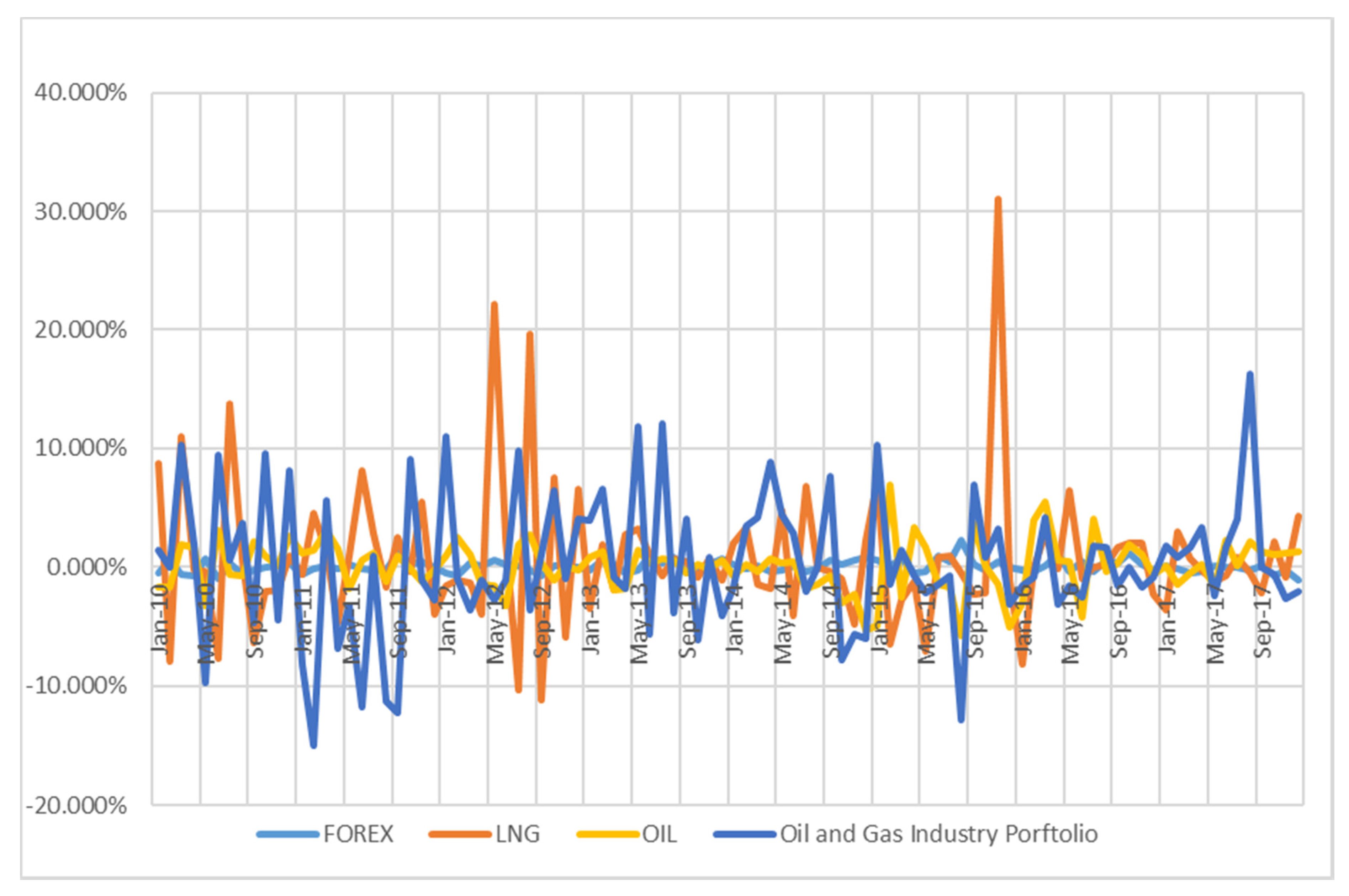
According to Basher and Sadorsky [2], the stock markets of emerging countries are highly volatile to oil price fluctuations, as authors argued that “emerging economies tend to be more energy intensive than more advanced economies and are therefore more exposed to higher oil prices. Consequently, oil price changes are likely to have greater impact on profits and stock prices of emerging economies.” (p. 226). Thus, being an emerging and oil and gas exporting country, the Malaysian stock market is very much exposed to the volatility of oil price. However, the intensity of exposures is comparatively high on oil and gas industry stock because the operating costs and profits of oil and gas firms are conditional to the fluctuation of oil and gas prices [10,11,12,13,14]. Thus, the behavior of oil and gas stocks is different from that of other stocks at persistent volatility of oil and gas price. Therefore, the volatility in oil and gas stock returns come not only from the general stock market fluctuations but also from the oil price and gas price volatility [10,11,12]. Additionally, if the firm operates in a net oil and gas exporting country, exchange rate also plays an important role in influencing energy stock prices to be more volatile. Moreover, oil and gas companies in Malaysia are price takers of international crude oil and gas prices [11,12]. Therefore, the cash flows and the stock prices of oil and gas companies are exposed to oil and gas price volatility [10,11,12,13,14]. Consequently, the unpredictable nature of oil prices always creates uncertainty in the economy and the oil and gas industry’s revenue generation. Hence, the unpredictable swings in oil and gas prices could affect the sector’s stock performance. In supporting those, Figure 1 also shows that oil and gas industry stock returns and exchange rate change move together, where oil and gas industry stock appreciates with a high margin in responding to a small amount of exchange rate depreciation, vice versa. Therefore, it can be said that oil price, gas prices, and exchange rate are significant risk factors for this industry’s stock prices and returns alongside the market-based risk factors.

Given the high volatility nature of oil prices and gas prices, the underlying return distributions for oil and gas stocks no longer tend to stay normal. The implication is that, if the underlying return distributions are not normal, the standard asset pricing models that employed in examining the effect of oil-related risk exposure on stock returns may not be able to adequately capture the variation in stock returns. These—the standard asset pricing models—were developed under the assumption that investor exhibits mean-variance behavior. They are thus bounded by the assumption of normal distribution in stock returns [15,16,17]. Hence, this circumstance motivates us to find a better framework that can explain the maximum variation and has a higher explanatory power. Henceforth, the examination of the relation between oil and gas returns and risk factors should be using the mean semi-variance framework proposed by Estrada [15], which is appropriate when the underlying return distribution is non-symmetrical or does not have a bell-shaped distribution.

Most past oil-related studies employ standard multifactor asset pricing models, which implicitly assume that the underlying distribution of returns is normal or symmetrical (e.g., [11,14,18,19], among others). While numerous prior studies recognize that stock returns are non-normally distributed especially within the context of emerging markets, at best, these studies only include additional risk measures to proxy for downside risk such as skewness and kurtosis in the analysis modelled using standard asset pricing model [2,20]. In those studies, the asset pricing framework and factor are still based on co-movements, and the inclusion of co-skewness and co-kurtosis are just non-linear effects of risk factors. So, they do not deal with individual stock returns distribution and their representation in the estimation. Given that, the semi-variance framework of asset pricing is totally different from others, as the framework allows us to adjust both the right and left side of the mathematical equation and facilitate the estimation considering risk factors that are included in the model.

From a different point of view, the existence of the high volatility in the stock market, oil price, gas price, and exchange rate returns create uncertainty and risk aversion in investor’s minds. In such a situation, before investing in the oil and gas sector, investors prefer safety first. It is also said that investors place greater weights on adverse conditions of the respective risk factor in their utility function (see [17,21,22]). Therefore, investors push the expected risk premium to up for taking downside risks that are involved with oil and gas risk factors. The empirical studies proved that the nexus of downside risk and stock return tend to be negative (e.g., [23,24,25]). They conclude the unfavorable conditions of respective risk factors will have negative impacts on stock performances. Hence, considering stock market, oil price, gas price, and exchange rate are important risk factors in oil and gas stock performance, it is important to investigate how the downside risk of oil price, gas price, and exchange rate risk factors are priced in oil and gas stock returns.

The objective of the current study is two fold, (i) investigating the link between oil-related risk factors and stock returns of Malaysian oil and gas companies employing a downside asset pricing framework; and (ii) investigating how downside risk of oil return, gas return, and exchange rate return are priced in oil and gas stock returns using two-stage cross-sectional estimations. Therefore, this paper contributes to the literature in several ways. Firstly, the contribution is related to the methodology which represents a more plausible method of assessing the impact of oil price and gas price risk exposure on oil and gas stocks in a non-normal return distribution condition resulted from oil price and gas price volatilities. This study employs a more refined method than the standard mean-variance approach in investigating the impact of oil-related risk factors on stock returns by employing a downside multifactor asset pricing model. In this paper, we show how the downside asset pricing framework modelled using the mean semi-variance approach helps to provide a better understanding of the link between oil-related risk factors and stock returns. The semi-deviation approach is modelled in a downside setting, which allows the incorporation of downside risk exposures to market risk, size factor, value factor, momentum factor, oil return, gas return, and exchange rate return. In this end, we closely follow the mean semi-variance approach proposed by Estrada [15] and the underlying justifications for its application. At this instance, our study extends the literature that related to mean semi-variance framework (e.g., [15,21,22]) and oil and gas stock (e.g., [11,12,14,23,24,26,27]).

Secondly, this paper contributes to the scant firm-level analysis on the relationship between oil-related risk factors and stock returns and expands understanding in the emerging market and Malaysian market context. The firm-level analysis is also important to understand the heterogeneity within the industry. The research on host subject matter has largely focused on developed markets with limited investigations conducted in the context of emerging and developing markets, especially the US and the UK market (e.g., [2,18,19,26,27]). The firm-level analysis of Malaysian oil and gas firms suggests that market, size, momentum, oil price, gas price, and exchange rate determinant of oil and gas stock returns, which contributes to oil and gas stock returns valuations and adds new literature in the Malaysian context. The empirical results of the firm-level analysis also reveal that the effects of risk factors on oil and gas firms are heterogenous in the oil-exporting country case. Additionally, our empirical results allow comparing the stocks regardless of their size and book-to-market value. Hence, our study offers new insights to researchers and practitioners about industry specificities related to the heterogeneous behavior of stocks. The current study also validates the findings of Mohanty and Nandha [27] and Sansui and Ahmed [19] improves the literature by showing gas price and exchange rate are influential factors to oil and gas firms. We suggest oil price, gas price, and exchange are systematic risk factors of oil and gas firm, alongside the market-based risk factors.

Thirdly, this paper contributes by documenting and presenting how exposures to the downside of oil and gas risk factors are priced in the cross-section of stock performance. Our findings for oil and gas companies draw attention to the importance of the downside in oil-related risk factors, as we evidence that downside risk exposures to risk factors are negatively priced in the Malaysian oil and gas stocks, apart from the gas (LNG) risk factor. The negative risk-return relationship was observed in numerous past studies that employ downside risk measures in the standard asset pricing models [20,22,23,28]. The findings of negative risk-return relationships in those studies have so far been regarded as “anomalies”, as it is assumed that investors are risk-averse, and thus demand compensation for bearing risk, which implicitly indicates a positive risk-return relationship. Unlike prior research, we show that the findings of the negative relationship between risk factors and stock returns are no longer unexpected and can be explained using the risk preference explanation of prospect theory by Kahneman and Tversky [29]. According to the authors, investors in the downside states implicitly perceive that they may be in a losing state or the domain of loss. Investors exhibit risk-seeking behaviors when facing with a loss-making domain and are thus penalized with low returns for their risk-seeking behaviors.

The remainder of this paper proceeds as follows. The following section discusses the relevant literature, and Section 3 provides data description and discussion of preliminary analysis. Section 4 describes the empirical methods employed in this study, and Section 5 presents empirical findings and discussions. Concluding remarks are provided in Section 6.

2. Theoretical Framework

2.1. Asset Pricing Model

In the case of oil and gas stock valuations, the arbitrage pricing theory (APT) is the most appropriate approach, which allows oil price, gas price, and exchange rate factors into the valuation. The theory facilitates modeling the expected returns of any financial asset as a linear function of various factors. Arbitrage pricing theory was originally developed by Stephen Ross [30] to explain the relationship between risk and returns, and it is formulated to capture stock return sensitivity to systematic risk factors. APT explains that several firms or security-specific factors can influence the stock price. The following equation expresses APT mathematically.

$$E\left(R_i\right)=rf+{\displaystyle \sum }_1^n{\beta }_n{f}_n+\epsilon$$

(1)

where $E\left(R_i\right)$ represent expected stock returns. $rf$ denotes risk free rate. ${\beta }_n$ signifies sensitivity to the n factor. $f_n$ represents price of the n factor. $\epsilon$ is unsystematic or idiosyncratic risk factors.

The empirical studies suggest that market factor, size factor, value factor, and momentum factor are important risk factors that can influence stock returns significantly (see [14,23,31,32]. As the APT recommends, there will be some firm or security-specific factors which can affect equity returns. This study, therefore, conjectures that Carhart risk factors and oil and gas industry-specific risk factors will have significant effects on oil and gas stock returns. There are several reasons to believe oil and gas industry-specific risk factors could have an influence on oil and gas stock prices. Firstly, investors believe that both oil and gas are primary inputs in the business operations of the oil and gas industry. Thus, changes in oil and gas prices directly affect oil and gas firm earnings and lead to change cash flows, which in turn act as inputs for stock valuation models. Therefore, oil and gas prices directly affect oil and gas stock prices (see [11,12,14,18,31,32]). Secondly, when investing in the oil and gas industry, investors carefully observe oil price fluctuations, because they believe that changes in oil price influence macroeconomic variables, such as interest rates, exchange rates, and commodity prices indirectly impact discounted cash flows and have a knock-on effect on stock prices. Thirdly, “volatility in oil prices can contribute to risk premiums required by investors on assets that have greater risk exposures concerning oil price fluctuations. Depending on the sign of the risk premium associated with a firm’s exposure to oil price, oil price sensitivity can positively or negatively affect stock prices” ([31], p. 132). Fourthly, exchange rate and oil price move together, and mostly exchange rate of net oil-exporting countries appreciates against positive oil price changes (see [33]). The exchange rate appreciation can negatively affect the oil and gas stock price of net oil-exporting countries, as exchange rate appreciation reduces oil and gas firms’ revenues and profits. So, stock prices experience downward trends that are unfavorable to stock returns. In addition, oil price leading exchange rate appreciation causes the export competitiveness of other sectors to fall, which can affect the stock price. Henceforth, the APT model for the current study is expressed as below.

$$E\left(R\right)=rf+{\beta }_{1}MKT+{\beta }_{2}SMB+{\beta }_{3}HML+{\beta }_{4}WML+{\beta }_{4}OIL+{\beta }_{5}GAS+{\beta }_{5}FOREX+\epsilon$$

(2)

where $E\left(R\right)$ represent expected stock returns. $rf$ denotes risk free rate. MKT, SMB, SMB, HML, OIL, GAS, and FOREX represents price of the stock market, size, value, momentum, oil price, gas price, and exchange rate risk factors, respectively. ${\beta }_1,$ ${\beta }_2,{\beta }_3,{\beta }_4,{\beta }_5,\mathrm{and}{\beta }_6,$ signify sensitivity to the stock market, size, value, momentum, oil price, gas price, and exchange rate risk factors, respectively. $\epsilon$ is unsystematic or idiosyncratic risk factors.

2.2. Mean Semi-Variance Framework

For a long time, the mean-variance theory (optimal portfolio theory) of Harry Markowitz [34] has been using for addressing the risk and return trade-off. This theory was formulated based on two standard assumptions: (i) the distribution of returns is normal, and (ii) the distribution of returns is symmetric [15,16,35]. “In this theory, investor’s decision formulates a trade-off between the return and the risk, in which the risk is measured by the variance of the returns” ([36] p. 315). In this framework, risks are measured by the standard deviation and the beta as shown in the following Equations (3) and (4), respectively:

$${\sigma }_{jt}=\sqrt{E{\left(R_{jt}-{\overline{R}}_j\right)}^2}$$

(3)

$$\beta =\frac{E\left[\left(R_{jt}-{\overline{R}}_j\right)\left(R_{mt}-{\overline{R}}_m\right)\right]}{E[{\left(R_{mt}-{\overline{R}}_m\right)}^2]}$$

(4)

where $R_{jt}$ and $R_{mt}$ are returns of each stock j and returns of market m for week t, respectively. ${\overline{R}}_j$ and ${\overline{R}}_m$ represents mean returns of stock j and market m, respectively. ${\sigma }_{jt}$ represents the standard deviation of returns or total risk, and ${\beta }_i$ represents beta or systematic risk for stock j. Henceforth, the equity returns can be calculated as follows,

$$R_j=rf+\mathrm{MRP}\ast \mathsf{\beta }$$

(5)

where $R_j$ represent stock returns. $rf$ denotes risk free rate. ${\beta }_o$ signifies sensitivity to the n factor. MRP represents risk premium, MRP = $E\left(R_m\right)-rf$. The following the regression model has been used to estimate risk coefficient ($\beta )$ under mean-variance framework.

$$R_{jt}-r{f}_t=\alpha +\mathsf{\beta }\left(R_{mt}-r{f}_t\right)+{\mathsf{\epsilon }}_t$$

(6)

where $R_{jt}-r{f}_t$ and $R_{mt}-r{f}_t$ denote stock excess returns and market excess returns, respectively.

Mean-variance theory, however, is often questioned for its downside risk in asset pricing, because investors are more concerned about downside risk than favorable upside risk [37]. It is believed that classic mean-variance theory does not consider investors’ rational preferences in asset pricing [38]. The rationality is that investor perceives not to lose the invested amount. Thus, investors put the twice-weight on losses as compared to gain [39]. These circumstances have led financial economists and academic practitioners to develop new pricing theory/framework for asset pricing and managing risk, in the form of downside risk measures. These theories include the lower-partial moment framework of Bawa and Lindenberg [17], the loss aversion of Kahneman and Tversky [29] in their prospect theory, the disappointment aversion of Gul [17], and the mean semi-variance framework of Estrada [15,20,40].

According to Harlow and Rao [41], a downside risk framework should be capable of facilitating less downside exposure while preserving the same or a greater level of expected return in asset pricing models. The rationality is that downside risk measure is consistent with the way investors perceive risk [42]. Though the computation of lower partial-moments is complex, Klebaner et al. [35] claimed that these are not cheaply-made measures, but based on theoretical, primitive, and instinctual features of capital market theories (see [17,41,43]).

Grounded on lower partial-moments of Bawa and Lindenberg [17] and Harlow and Rao [41], Estrada [15,35,40,44,45,46] proposed a mean semi-variance framework for asset pricing that even resolves the benchmarking problem of target returns. In Estrada’s [15] mean semi-variance framework mean returns are used as a benchmark for calculating lower partial moments. His asset pricing approach under mean semi-variance outperforms the mean-variance approach in certain conditions (distribution of returns is not normal and symmetric in a highly volatile market). The lower partial-moments framework is suggesting that the current study should employ mean semi-variance of Estrada [15] as high volatilities are associated with oil and gas stock returns and risk factors. The following Equations (7) and (8) can be applied to measure semi-deviation and downside beta.

$${\Sigma }_{jt}=\sqrt{Emin{\left[\left(R_{jt}-{\overline{R}}_j\right),0\right]}^2}$$

(7)

$${\beta }^D=\frac{E\left\{\min \left[\left(R_{jt}-{\overline{R}}_j\right),0\right]\min \left[\left(R_{mt}-{\overline{R}}_m\right),0\right]\right\}}{{\left[Emin\left(R_{mt}-{\overline{R}}_m\right),0\right]}^2}$$

(8)

where $R_{jt}$ and $R_{mt}$ are returns of each company j and returns of market m for week t, respectively. ${\overline{R}}_j$ and ${\overline{R}}_m$ indicates mean returns of company j and market m, respectively. ${\Sigma }_{jt}$ is the semi-deviation of returns or the downside of standard deviation of returns. ${\beta }^D$ represents down beta for company j. Estrada [8] suggest D-CAPM can be estimated with regression without intercept, which is shown below.

$$[Min\{(R_{jt}-{\overline{R}}_j),0\}]={\beta }^D\left[\min \left\{\left(R_{mt}-{\overline{R}}_M\right),0\right\}\right]+{\mathsf{\epsilon }}_t$$

(9)

The above-mentioned theories state that downside risks should be priced into expected stock returns. Notably, “the loss aversion utility function of Kahneman and Tversky [29] suggests investors will place a relatively greater weight on avoiding losses, implying that downside risk may be priced” ([20], p. 4336). These behavioral finance theories suggest that investors should be rewarded for downside risk. Aligning these arguments, a group of researchers proved that aversion to losses lead investors to seek additional risk premium for bearing downside risks [47,48,49,50]). Furthermore, they also suggest that loss-aversion for particular stock returns explains the higher volatility of stock returns observed in the market [51,52]. The implication is that downside risk measures are appropriate in explaining stock returns with investor loss-aversion function. On the other hand, in line with prospect theory, Alles and Murray [20] argued that risk-seeking behavior for downside risk is sometimes penalized, and the risk-return relationship also depends on the phase of the stock market.

The high volatility in stock market, oil price, gas price, and exchange rate returns create uncertainty and risk aversion in investor’s minds. In such a situation, before investing in the oil and gas sector, investors prefer safety first. The fact is that investors always want to avoid the downside of risk factors as those risks can affect stock price and stock market negatively. Theoretically, investors place greater weights on adverse conditions of the respective risk factor in their utility function (see [17,21]). They conclude the unfavorable condition of respective risk factors will have negative impacts on stock performances. Hence, considering stock market, oil price, gas price, and exchange rate are important risk factors in oil and gas stock performance, the theoretical implications are suggesting that the current study should employ downside risk as a proxy for risk to observe how loss-aversion and risk-seeking behavior of investor rewarded or penalized for downside risk in oil and gas stocks.

3. Related Studies to Oil and Gas Stock

While there are numerous studies that investigate the impact of oil prices on firm-level stock returns, most studies examine the relationships in time-series setting. Sadorsky [53] examines the responses of Canadian oil and gas stocks to the fluctuation in oil prices using a multifactor model and find that changes in crude oil price have a significant positive impact on the returns of oil and gas stocks. Lanza et al. [54] examines the impacts of common driving factors such as market, exchange rate, and spread of oil price on the stock prices of six major oil companies. Their findings indicate that changes in oil price and exchange rate have a significant impact on oil stock returns. Jin and Jorion [55] explore the relationship between stock return sensitivity of oil and gas producers and commodity prices. They find evidence that oil and gas prices have a significant positive effect on firm value. Boyer and Filion [28] report that crude oil prices and natural gas prices have significant positive impacts on the stock returns of Canadian oil and gas companies. Sadorsky [56] investigates the impact of global oil market risk factors on oil price risk and oil companies’ stock prices. The findings show that oil price risk is negatively affected by increases in oil reserves and positively affected by increases in oil production.

Sadorsky [57] examines oil price effects on stock prices of companies with different sizes and finds that the impacts are size-dependent with the strongest impacts observed for medium-sized companies. Kretzschmar and Kirchner [58] investigate risk factors and reserve location effects on the returns of oil and gas companies. After controlling for Fama and French risk factors, the results indicate that reserve location has positive and asymmetric effects on oil and gas stock returns. Mohanty and Nanda [27] examine the impacts of oil shocks on stock returns of the US oil and gas sector using an augmented four-factor asset pricing model. They find that various risk factors such as oil price changes, market, book-to-market, size, and momentum factors are significant return determinants of the oil and gas sector. Using a multi-factor asset pricing model, Sanusi and Ahmad [19] examine the determinants of oil and gas stock returns in the UK and find that oil-related risk factors such as market, oil price, size, and book-to-market risk factors are significant determinants of stock returns for oil and gas companies. Using firm-level data, Demirer et al. [31] examine whether oil price risks are priced in the cross-section of stock returns in net oil-exporting countries of Gulf Arab stock markets. They find no evidence that oil price risk is associated with significant risk premium after controlling for firm-level risk factors. Using asset pricing models, Hoque et al. [11,12] have found oil and gas risk factors influence Malaysian oil and gas stock returns asymmetrically and heterogeneously depending on the sub-sector and the time.

Scholtens and Wang [59] investigate the cross-section relation between oil and gas risk factors and stock returns using a two-stage regression approach and a multifactor pricing model. They find that risk factors such as market, book-to-market value, and changes in oil prices are positively priced in the cross-section of oil and gas stocks. Ramos et al. [32] find that the oil price risk factor is positively priced in oil and gas stock returns, and hence is a systematic risk factor. The studies of Scholtens and Wang [51] and Ramos et al. [32] employ data from the U.S., an oil-importing country. Hence, their results and implications cannot be generalized to the oil and gas industry of exporting and emerging markets. Furthermore, so far, none of the extant empirical studies has investigated the effects of oil-related risk factors on stock market returns using the mean semi-variance framework, which is the major strength of the present study.

4. Empirical Framework

4.1. A Baseline Model under Mean-Variance Framework

Based on asset pricing theory discussed in Section 2.1, the present study formulates a baseline multifactor asset pricing model under the mean-variance framework, which is presented in Equation (10). This baseline model will be considered in developing downside version of asset pricing model.

$$\begin{gathered} (R_{jt}-r_{ft})={\alpha }_j+{\beta }_{0,\mathrm{j}}\left(R_{mt}-r_{ft}\right)+{\beta }_{1,\mathrm{j}}SM{B}_t+{\beta }_{2,\mathrm{j}}HM{L}_t+{\beta }_{3,\mathrm{j}}\mathrm{WML}+{\beta }_{4,\mathrm{j}}∆OilPric{e}_t \\ +{\beta }_{5,\mathrm{j}}∆LNGpric{e}_t+{\beta }_{6,\mathrm{j}}∆FORE{X}_t+{\epsilon }_{jt};j=1,\dots ,J;t=1,\dots ,T. \end{gathered}$$

(10)

where $R_{jt}$ are returns of each company j for week t. $rf$ is the risk-free rate for week t. $R_{mt}$ is the return of the market portfolio for each week. The variables SMB, HML, and WML are the respective size, book to market value, and momentum factors. $∆OilPrice$, $∆LNGprice$, and $∆\mathrm{FOREX}$ are log changes in oil prices, LNG prices, and exchange rates, respectively. ${\mathsf{\epsilon }}_{\mathrm{jt}}$ is the pricing error. The coefficient ${\beta }_{0,j}$ captures the return sensitivity of company j to market fluctuation. ${\beta }_{1,j},{\beta }_{2,j}\mathrm{and}{\beta }_{3,j}$ represent returns sensitivity to the size, book to market value, and momentum factors respectively for company j.${\beta }_{4,j}$ and ${\beta }_{5,j}$ denote return sensitivity to oil price and gas price variation respectively for company j. ${\beta }_{6,j}$ is the return sensitivity to exchange rate uncertainty for company j.

4.2. Multifactor Asset Pricing Model under the Mean Semi-Variance Framework

According to Estrada [15], the simplest and most appropriate way of obtaining a downside coefficient is through running a standard linear regression model without a constant term. Thus, the present study considers a multifactor asset pricing model without a constant term. Henceforth, we re-formulate Equation (10) into a new multifactor asset pricing model under the mean semi-variance framework, which is also known as the downside multifactor asset pricing model.

$$\begin{gathered} [Min\{(R_{jt}-{\overline{R}}_j),0\}]={\beta }_{0,j}^D\left[min\left\{\left(R_{mt}-{\overline{R}}_M\right),0\right\}\right]+{\beta }_{1,j}^D\left[min\left\{\left(SM{B}_t-\overline{SMB}\right),0\right\}\right]+ \\ {\beta }_{2,j}^D\left[min\left\{\left(HM{L}_t-\overline{HML}\right),0\right\}\right]+{\beta }_{3,j}^D\left[min\left\{\left(WM{L}_t-\overline{WML}\right),0\right\}\right]+ \\ {\beta }_{4,j}^D\left[min\left\{\left(∆OilPric{e}_t-\overline{∆OilPrice}\right),0\right\}\right]+{\beta }_{5,j}^D[min\{(∆LNGpric{e}_t- \\ \overline{∆LNGprice}),0\}+{\beta }_{6,j}^D\left[min\left\{\left(∆FORE{X}_t-\overline{∆FOREX}\right),0\right\}\right]+{\epsilon }_{jt}j=1,\dots ,J;t=1,\dots T \end{gathered}$$

(11)

where $R_{jt}$ is the return of each company j for week t. $R_{mt}$ is the return of the market portfolio for week t. The variables SMB, HML, and WML are size, book to market value, and momentum factors, respectively. The variables ∆OilPrice, ∆LNGprice, and ∆FOREX represent log changes in oil prices, LNG prices, and exchange rates, respectively.${\overline{R}}_j$, ${\overline{R}}_M$, $\overline{SMB}$, $\overline{HML}$, $\overline{WML}$, $\overline{∆OilPrice}$, $\overline{∆LNGprice}$, and $\overline{∆FOREX}$ represent the mean returns of the respective variables. ${\epsilon }_{jt}$ is the pricing error.

4.3. Downside Multifactor Asset Pricing Models with a Two-Pass Regression

A standard two-pass regression is considered to investigate the cross-sectional relationship between risk and returns, as Goyal [60] and Kan and Robotti [61] indicate that a simple two-pass regression is easier to manage. Additionally, Low et al. [62], among others, have also employed a simple two-pass regression for examining the cross-sectional relation between a country’s stock market returns and governance quality. In the present study, we apply a standard two-pass regression for examining the effects of downside exposure of oil and gas risk factors on the cross-section returns of oil and gas stocks. This second stage estimation is important for knowing whether or not oil and gas stock investors require oil-related risk premiums (The first stage estimation only shows how risk factors affect stock returns, while the second stage estimation shows how risks are being priced in stock returns.).

In the first stage, for each company, a time series ordinary least square (OLS) regression is performed to estimate the effects of risk factors on the returns of oil and gas companies. The regression models are specified under the mean semi-variance framework, as shown in Equation (11). In the second stage, the coefficients will obtain from the first-stage time series regression are employed as independent variables in the second-stage cross-sectional regressions. We perform two different cross-sectional regressions, using an average excess return of stocks and total risk exposure as a dependent variable.

When a firm’s total risk exposure is used as a dependent variable, we examine the role of downside exposure to oil and gas risk factors in the cross-section of total risk for oil and gas stocks. For the dependent variable, we use two measures to proxy for a company’s total risk exposure, namely the standard deviation of returns and the semi-deviation of returns for stocks. The cross-sectional regression model is specified as follows in Equation (12) (Following Tse [63], the present study also excludes constant term in the second stage cross-sectional regressions.).

$$\begin{gathered} {\gamma }_j={\psi }_1\left({{\beta }_j^D}^{MKT}\right)+{\psi }_2\left({{\beta }_j^D}^{SMB}\right)+{\psi }_3\left({{\beta }_j^D}^{HML}\right)+{\psi }_4\left({{\beta }_j^D}^{WML}\right)+{\psi }_5\left({{\beta }_j^D}^{OIL}\right)+ \\ {\psi }_6\left({{\beta }_j^D}^{LNG}\right)+{\psi }_7\left({{\beta }_i^D}^{FOREX}\right)+{\epsilon }_{j}j=1,\dots .,J. \end{gathered}$$

(12)

where ${\gamma }_j$ is the risk measures employed for stock j. ${\psi }_j$ represent vectors of downside risk coefficient estimated from the first-stage time series regression model. ${\epsilon }_j$ is the pricing error.

In the following cross-sectional regression model as specified in Equation (13), we employ average excess stock returns as a dependent variable, and as before, the independent variables are downside risk coefficients obtained from the first-stage time series regression. We examine if downside exposures to oil and gas risk factors are priced in the cross-section of oil and gas stocks.

$$\begin{gathered} {\vartheta }_j={\theta }_1\left({{\beta }_j^D}^{MKT}\right)+{\theta }_2\left({{\beta }_j^D}^{SMB}\right)+{\theta }_3\left({{\beta }_j^D}^{HML}\right)+{\theta }_4\left({{\beta }_j^D}^{WML}\right)+{\theta }_5\left({{\beta }_j^D}^{OIL}\right)+ \\ {\theta }_6\left({{\beta }_j^D}^{LNG}\right)+{\theta }_7\left({{\beta }_i^D}^{FOREX}\right)+{\epsilon }_{j}j=1,\dots .,J. \end{gathered}$$

(13)

where, ${\vartheta }_j$ represents average excess return.$\theta$_j are vectors of downside coefficient estimates obtained from the first-stage time series regression estimation. ${\epsilon }_j$ is the pricing error.

5. Dataset Description and Preliminary Analysis

The study sample comprises publicly listed oil and gas companies in the stock exchange of Malaysia. The sample period consists of weekly data from Monday to Friday, from January 2010 to December 2017, totalling 417 weeks. The present study selects companies based on the unbroken series of returns and historical closing prices to minimize survivorship bias. Based on the screening, the study sample comprises 33 oil and gas stocks from Bursa Malaysia. The sample size of the current study is larger than those of Lanza [50]), and Sanusi and Ahmad [19], which consist of 6 and 30 companies, respectively. While the sample size of this study is smaller than those of Biyor and Filion [26], Kretzschamar and Kirchner [58], and Ramos and Veiga [14] this study employs weekly frequency data, and thus has a larger observation size. Unlike the present study, those past studies have ignored the gas price risk premium in their analyses.

Firm-level data of 33 oil and gas stocks, capital gain, and dividend-adjusted historical closing stock prices, were extracted from the websites of Bursa Malaysia and Yahoo Finance. FTSE Bursa Malaysia KLCI serves as the market proxy. The data on 90 days T-bill rate, a proxy for the risk-free rate, were obtained from the Bank Negara website. Weekly oil prices and gas (LNG) prices were compiled from the Energy International Administration’s website and DataStream. The current study uses international crude oil prices and international gas (LNG) prices instead of national-level prices. The changes in the world oil prices have stronger impacts on the stock market than changes in the national level oil prices [12]. Exchanges rate—which is the unit of Malaysian ringgit against the unit of U.S. dollar—data were extracted from the website of Bank Negara and DataStream.

Construction of Size (SMB), Book-to-Market (HML), and Momentum (WML) Factors

For constructing a small-minus-big portfolio (SMB, hereafter) and a high-minus-low portfolio (HML, hereafter), this study follows the procedure of Fama and French [64]. The study forms SMB and HML factors using a two-by-three sorting procedure based on size and book-to-market ratio. All stocks are ranked based on their market capitalizations in defining the size grouping of stocks. Based on the median value of market capitalization, two groups of portfolios are formed: small stocks portfolio and big stocks portfolio. Similarly, using the book-to-market ratio, all stocks are ranked and sorted into three groups where the top 30%, middle 40%, and bottom 30% of the book-to-market ratios are defined as high, medium, and low book-to-market portfolios, respectively.

After sorting the two size portfolios and three book-to-market portfolios, the intersections of these portfolios resulted in the formation of six portfolios. These equally weighted portfolios are small-low (SL), small-medium (SM), small-high (SH), big-low (BL), big-medium (BM), and big-high (BH). The SMB factor is defined as the average for the difference between small portfolios and big portfolios for each week. On the other hand, the HML factor is defined as the average for the difference between high portfolios and low portfolios for each week. The following Equations (14) and (15) are used for obtaining SMB and HML factors, respectively.

$$\mathrm{SMB}=\frac{1}{3}\left\{\right(\mathrm{SL}+\mathrm{SM}+\mathrm{SH})-(\mathrm{BL}+\mathrm{BM}+\mathrm{BH}\left)\right\}$$

(14)

$$\mathrm{HML}=\frac{1}{2}\left\{\right(\mathrm{SH}+\mathrm{BH})-(\mathrm{SL}+\mathrm{BL}\left)\right\}$$

(15)

Jegadeesh and Titman [65] introduce the momentum factor (WML, hereafter) to capture anomalies related to the momentum of stock returns. In order to generate the WML factor, this study follows the study of Fama and French [66]. This study separates all stocks into three groups based on cumulative momentum returns of month 12 (which is equivalent to week 52 in this study) and month 2 (which is equivalent to week 5 in this study) during portfolios formation, where the top 30%, middle 40%, and bottom 30% of the book-to-market values are defined as winners, losers, and neutral portfolios, respectively. After sorting, the intersections of size and momentum portfolios resulted in the formation of six portfolios—such as small-loser (SL), small-neutral (SN), small-winner (SW), big-loser (BL), big neutral (BN), and big-winner (BW). Henceforth, the WML factor can be obtained from the difference between the average returns on winner portfolios and the loser portfolios. The following Equation (16) is used for obtaining the WML factor.

$$\mathrm{WML}=\frac{1}{2}\left\{\right(\mathrm{SW}+\mathrm{BW})-(\mathrm{SL}+\mathrm{BL}\left)\right\}$$

(16)

6. Empirical Results and Discussion

6.1. Preliminary Analysis

Table 1. Descriptive Statistics and Normality Test of Oil and Gas Stock Returns and Risk Factors.

	Mean	Annualized Mean	Total Risk	Downside Total Risk	DR/TR	Skewness	Kurtosis	Jarque−Bera	Probability
Panel A: Oil and Gas Stock
Alam Maritime Resources	−0.002	−0.017	0.382	0.238	62%	−0.198	12.092	1439.04	0.000
Bumi Armada	0.176	1.267	1.234	0.638	52%	1.271	3.207	91.329	0.000
Carimin Petroleum	−0.005	−0.036	0.517	0.252	49%	2.403	18.311	1759.85	0.000
CLIQ Energy	−0.001	−0.004	0.491	0.256	52%	2.80	13.41	75.881	0.000
Dayang	0.001	0.009	0.371	0.238	64%	0.500	6.950	288.463	0.000
Deleum	−0.003	−0.018	0.384	0.238	62%	−0.173	11.861	1376.15	0.000
E.A Technology	0.000	0.000	0.461	0.271	59%	0.110	4.231	10.486	0.005
Gas Malaysia	0.001	0.008	0.202	0.134	66%	−0.849	7.741	311.723	0.000
Handal Resources	−0.002	−0.012	0.417	0.250	60%	−0.304	10.138	865.982	0.000
Heng Huat	−0.001	−0.004	0.424	0.232	55%	0.556	4.450	25.038	0.000
Hibiscus Petroleum	0.003	0.023	0.552	0.305	55%	0.701	8.978	527.872	0.000
ICON Offshore	−0.009	−0.068	0.451	0.271	60%	0.103	6.159	76.833	0.000
Kejuruteraan Samudra Timur	0.001	0.006	0.519	0.283	55%	1.200	12.392	1632.68	0.000
KMN	−0.004	−0.032	0.473	0.257	54%	0.936	8.819	649.285	0.000
KUB MY	0.001	0.005	0.377	0.186	49%	1.344	7.930	547.817	0.000
Perdana	0.005	0.033	0.384	0.217	57%	0.305	4.791	62.196	0.000
Perisai Petroleum	−0.005	−0.035	0.621	0.387	62%	0.738	15.260	2649.37	0.000
Perton	0.005	0.034	0.316	0.152	48%	2.000	14.443	2553.19	0.000
Petra Energy	0.000	−0.003	0.391	0.218	56%	0.958	10.289	986.829	0.000
Petronas Dagangan Bhd	0.003	0.020	0.196	0.127	65%	−0.555	6.651	252.950	0.000
Petronas Gas	0.001	0.006	0.519	0.283	55%	1.200	12.392	1632.68	0.000
SapuraKencana	−0.003	−0.018	0.410	0.275	67%	−1.139	12.366	1138.26	0.000
Scomi Energy	−0.002	−0.011	0.500	0.265	53%	1.147	12.154	1547.47	0.000
Scomi Group	−0.001	−0.004	0.595	0.411	69%	−2.134	73.179	85,890	0.000
Shell	0.001	0.009	0.288	0.171	59%	0.232	14.887	2458.96	0.000
Slik	0.000	−0.002	0.459	0.279	61%	0.430	19.285	4620.77	0.000
Sona Petroleum	0.001	0.008	0.236	0.144	61%	−0.073	7.244	173.575	0.000
Sumatec Resources Berhad	−0.002	−0.014	0.517	0.436	84%	1.576	22.814	6993.82	0.000
Tanjung Offshore	0.001	0.008	0.821	0.281	34%	1.414	12.577	1732.80	0.000
TH Heavy Engineering	−0.002	−0.012	0.703	0.357	51%	1.928	15.177	2834.84	0.000
UMW	−0.009	−0.062	0.483	0.300	62%	−0.091	10.262	479.366	0.000
UZMA	0.003	0.020	0.396	0.213	54%	0.607	4.936	90.720	0.000
Wah Seong	−0.001	−0.007	0.275		58%	0.556	6.992	298.461	0.000
Average	0.005	0.033	0.451	0.270	60%	0.813	5.904	651.5815	0.000
Panel B: Risk Factors
Market	0.000	0.003	0.093	0.059	63.44%	−0.165	4.964	68.899	0.000
SMB	0.009	0.068	1.295			−1.690	21.211	5960.437	0.000
HML	0.014	0.103	1.699			6.407	84.344	117,821.50	0.000
WML	0.069	0.495	0.446			−1.072	8.455	596.94	0.000
OIL	0.000	0.001	0.300			−0.262	4.486	43.143	0.000
LNG	0.007	0.053	0.932			5.443	61.142	60,794.960	0.000
FOREX	0.001	0.004	0.080			0.113	5.232	87.469	0.000

This table reports the results of the normality test along and summary statistics. The test results indicate whether stock returns are normally distributed. Column 1 lists companies in the oil and gas sector. Column 2 and 3 report the respective mean and annualized mean returns of companies over the sample period, respectively. Column 4 and 5 report the standard deviation and semi-deviation of stock returns, respectively. Column 6 shows the likelihood of downside volatility as indicated by the ratio of total downside risk to total risk (DR/TR). Columns 7 through 9 report Jarque−Bera (JB) test results estimated for each stock as JB:N[s2/6+(k − 3)2/24], where the respective s, k, and N are the values of skewness, kurtosis, and the number of data applied for the test, respectively. Column 10 shows the p-value of the Jarque−Bera test. In Panel B, the variable market represents the market excess return; small-minus-big portfolio (SMB), high-minus-low portfolio (HML), and WML are size, value, and momentum risk factors, respectively and; OIL, LNG, and FOREX represent price changes of oil, gas, and exchange rate, respectively.

presents summary statistics and normality test results for stock returns and risk factors of the Malaysian oil and gas industry over the study period. In the discussion, we outline several reasons for which semi-variance (or semi-deviation) of returns is a better measure of risk than variance (or standard deviation) of returns to justify the use of the mean semi-variance framework in analyzing the relationship between risk factors and stock returns of oil and gas companies. The volatility of oil and gas stock returns, measured by the standard deviation of returns which is the most widely accepted definition of total risk, is reported to be four times higher than that of the market return. That is, on average, the standard deviation of returns for oil and gas stocks is 40.10 percent, whereas the standard deviation of returns for the market is only 9.30 percent. In terms of downside risk, as measured by the semi-deviation of returns for oil and gas stocks, the average figure is 27 percent, whereas that of the market is 5.90 percent. The implication is that most of the oil and gas stocks have a relatively higher proportion of downside risk as shown by the ratio downside total risk to total risk (DR/TR). More specifically, there are five oil and gas stocks, in the study sample, which have total risk comprising more than 65 percent of the downside risk component. In addition to the highly volatile nature of oil and gas stock returns as established in the literature, the presented descriptive results also suggest that the mean semi-variance framework seems more plausible than the standard mean-variance framework in examining the returns of oil and gas stocks.

As reported in Table 1, some companies exhibit negative annualized mean returns and negative skewness of returns. This also suggests that the mean semi-variance framework is more appropriate to be employed than the mean-variance framework for asset pricing purposes. According to Sortino [67], if the stock return distributions are negatively skewed, downside risks are likely to be associated with the stock returns, and thus the downside risk framework is more appropriate to be employed than the standard mean-variance framework. On normality test results, based on the cut-off value of 3.00 for Kurtosis, the findings show that more than two-thirds of the companies have leptokurtic distributions, indicating that return distributions are not normal. Furthermore, using the normality test of the Jarque−Bera statistic, the current study finds that the returns of all companies and the returns of the market are not normally distributed. That is, the Jarque−Bera statistic confirms that the return distributions of companies and the market do not fulfill the normality assumption. Additionally, as reported in Panel B, the risk factors data also exhibit non-normal distributional property. Based on the above discussions, the current study employs the mean semi-variance framework for analyzing both the time series and cross-section of oil and gas stock returns. As discussed in Estrada [15,35,40,44,45,46], the mean semi-variance framework is particularly relevant for emerging markets. Collectively, the findings in the mentioned studies show the superiority of downside risk measures (semi-deviation of returns and downside beta) over the standard deviation of returns and beta in explaining the cross-section of stock returns in emerging markets.

Table 2. Summary Statistics of Variables.

	Average	Standard Deviation	Median	Minimum	Maximum
Total risk	0.4069	0.1392	0.4173	0.165	0.846
Downside total risk	0.2338	0.0830	0.2319	0.091	0.482
Average excess return	−0.0058	0.1556	0.0004	−0.172	0.015
Market	0.000	0.093	0.0010	−0.051	0.047
SMB	0.009	1.295	−0.0019	−0.086	0.1388
HML	0.014	1.699	−0.0013	−0.149	0.1387
WML	0.068	0.446	0.101	−2.875	1.403
OIL	0.000	0.300	−0.0005	−0.169	0.153
LNG	0.007	0.932	0.0000	−0.516	1.552
FOREX	0.001	0.080	0.0003	−0.054	0.044

This table reports summary statistics for total risk (standard deviation), downside total risk (semi-deviation), excess return, and risk factors. The variable market represents the market excess return; SMB, HML, and WML are size, value, and momentum risk factors, respectively; OIL, LNG, and FOREX represent price changes of oil, gas, and exchange rate, respectively.

presents summary statistics for variables employed in the study. On risk measures, the downside total risk, measured by semi deviation of returns, which comprises more than half of the total volatility of oil and gas returns. For example, the average value for downside total risk is 23.38 percent compared to that of 40.69 percent for total risk. The LNG risk factor is shown to be the most volatile oil-related risk factor with the highest standard deviation value of 93.2 percent, whereas exchange rate is the least volatile factor with a standard deviation of 8 percent. It is also reported that the volatility in oil and gas returns of 13.92 percent is higher than the volatility in market return which has a standard deviation of 9.3 percent. Additionally, it is observed that oil and gas companies have an average negative excess return of 0.58 percent.

Table 3. Correlation Matrix for Risk Factors.

Market	SMB	HML	WML	OIL	LNG	FOREX
1	−0.009 *	0.282 **	0.218 **	0.281 ***	0.044	−0.199 **	Market
	1	−0.301 **	−0.196 **	0.177 **	0.090 *	−0.092 *	SMB
		1	0.221 **	0.188 **	0.004	−0.186 **	HML
			1	0.331 **	0.207 **	−0.208 **	WML
				1	0.116 *	−0.442 **	OIL
					1	0.076 *	LNG
						1	FOREX

This table reports pairwise correlation coefficients between risk factors: market, SMB, HML, WML OIL, LNG, and FOREX. The variable market represents the market excess return; SMB, HML, and WML are size, value, and momentum risk factors, respectively; OIL, LNG, and FOREX represent price changes of oil, gas, and exchange rate, respectively. *, ** and *** denote statistical significance at 10%, 5%, and 1% levels, respectively. This table is published in our previous studies.

presents a correlation matrix for oil and gas risk factors and independent variables to provide a preliminary understanding of the relationship among the variables. The findings show that market risk factor is positively associated with oil price and gas price factors, while negatively related to the exchange rate factor. Overall, the reported correlation values are low, apart from the correlation between changes in oil price and exchange rate factor, which has a significant negative coefficient of 0.422. The market risk factor has significant correlation coefficients of 0.281 with changes in oil prices and of −0.199 with exchange rate changes. Interestingly, the market risk factor is shown to be uncorrelated with changes in LNG prices. This suggests that the LNG risk factor constitutes a firm’s unique risk which can be eliminated through diversification.

This study employs augmented Dickey–Fuller (ADF) and Phillip Perron (PP) unit root tests to check stationary in the data series (the results of ADF and PP unit root tests for oil and gas companies and risk factors will be provided upon request). The ADF and PP unit root test results suggest that all the returns series are stationary at the level form. Hence, this study needs not to employ co-integrated regression in the estimation process, and simple single equation models are sufficient to examine the relationships.

6.2. Downside Multifactor Asset Pricing Model—First Stage Time Series Regression

Table 4. Results of Time Series Regression under Mean Semi-Variance Framework (Downside Risk Model).

	MKT	SMB	HML	WML	OIL	LNG	FOREX	Rho	Adj-R sq	F Value	DW
Alam Maritime Resources	1.989 (5.35) ***	−0.006 (−1.97) **	−0.001 (−0.081)	0.005 (1.60)	0.215 (3.96) ***	−0.012 (−0.726)	0.416 (3.60) ***		0.4097	23.09 ***	1.95
BumiArmada	1.554 (4.96) ***	−0.096 (−5.43) ***	−0.013 (−1.18)	0.118 (8.85) ***	1.541 (7.28) ***	0.223 (3.23) ***	0.67 (5.14) ***		0.4721	48.41 ***	1.89
Carimin Petroleum	0.871 (3.59) ***	0.008 (0.62)	0.062 (2.66) ***	−0.009 (−0.55)	0.300 (3.84) ***	−0.051 (−1.36)	1.22 (2.48) **		0.2954	15.12 ***	1.90
CLIQ Energy	1.023 (3.19) ***	0.213 (2.08) **	0.062 (2.66) ***	0.003 (0.62)	0.168 (2.26) **	0.037 (1.58)	0.386 (2.61) **		0.2911	9.27 ***	1.98
Dayang	1.921 (9.11) ***	0.024 (2.12) **	0.014 (0.12)	0.018 (1.73) *	0.269 (4.13) ***	0.055 (1.68) *	0.404 (3.14) ***		0.6234	51.82 ***	1.99
Deleum	0.456 (2.23) ***	0.012 (0.79)	0.035 (3.20) ***	0.008 (2.19) **	0.133 (2.14) **	0.028 (1.99) **	0.830 (3.55) ***	0.112	0.1162	11.42 ***	2.01
E.A Techn	2.087 (2.34) **	0.038 (2.87) ***	0.035 (2.14) **	−0.016 (−1.13)	0.165 (2.48) **	0.054 (0.72)	0.62 (1.83)		0.3356	9.07 ***	1.91
Gas Malaysia	0.152 (188) *	0.016 (3.69) **	0.007 (1.49)	0.002 (0.70)	0.131 (2.11) **	0.016 (1.20)	0.558 (4.40) **		0.2809	13.93 ***	2.03
Handal Resources	1.550 (4.28) ***	0.007 (0.90) **	0.035 (2.12) **	0.009 (2.37) **	0.143 (3.17) ***	0.047 (1.88) *	0.602 (2.51) **		0.3170	23.56 ***	2.10
Heng Huat	1.606 (4.53) ***	0.003 (0.26)	0.029 (2.01) **	0.008 (0.57)	0.141 (2.64) **	0.113 (2.205) **	0.362 (1.16)	0.829	0.3037	12.01 ***	1.95
Hibiscus Petroleum	1.751 (4.63) ***	0.033 (2.66) ***	−0.008 (−0.84)	0.015 (3.28) ***	0.326 (5.64) **	0.033 (0.612)	0.784 (2.90) **	0.126	0.4522	20.86 ***	2.15
ICON OFFSHORE	1.534 (4.10) ***	−0.00 (−0.25)	0.013 (1.482)	0.031 (1.78) *	0.216 (2.58) **	−0.047 (−0.89)	0.193 (0.48)	0.011	0.2856	10.67 ***	2.01
Kejuruteraan SamudraTimur	0.989 (3.48) ***	0.023 (2.44) ***	0.018 (1.27)	0.004 (0.96)	0.268 (3.19) ***	0.036 (1.32)	1.308 (3.38) ***		0.1812	13.89 ***	1.89
KMN	1.917 (8.65) ***	0.006 (0.90)	0.044 (2.39) **	0.001 (0.07)	0.258 (3.23) ***	0.058 (2.41) **	0.459 (2.46) **		0.2875	24.69 ***	1.94
Perdana	0.435 (1.84) *	0.007 (0.81)	0.042 (2.99) ***	0.006 (1.57)	0.176 (3.63) ***	0.092 (2.68) ***	0.779 (3.11) **	0.241	0.1719	10.497 ***	2.02
Perisai Petroleum	2.279 (5.95) ***	0.076 (2.84) ***	0.079 (2.00) **	−0.003 (−0.80)	0.223 (2.99) **	0.056 (1.20)	0.281 (1.58)		0.4358	17.26 ***	1.96
Perton	0.503 (3.33) ***	0.005 (0.92)	0.041 (3.84) ***	0.008 (3.63) ***	0.109 (2.75) ***	0.007 (0.67)	0.516 (3.85) ***	0.172	0.2812	13.92 ***	2.01
Pertonas Gas	1.538 (6.68) ***	0.019 (1.93) *	0.024 (1.55)	0.006 (1.31)	0.266 (5.31) ***	−0.018 (−1.28)	0.561 (3.01) ***		0.2924	21.27 ***	1.94
Petra Energy	0.666 (4.54) ***	0.001 (0.045)	0.007 (1.70) *	0.007 (2.57) **	0.082 (3.13) ***	0.023 (0.25)	0.21 (1.96) **		0.3475	16.42 ***	1.89
Petronas Dagangan Bhd	0.989 (3.48) ***	0.023 (1.44)	0.018 (1.27)	0.004 (0.96)	0.268 (3.19) ***	0.036 (1.32)	1.308 (3.38) ***		0.3812	13.89 ***	1.94
SapuraKencana	2.538 (7.12) ***	0.014 (1.190)	0.038 (1.00)	0.003 (0.89)	0.172 (2.88) ***	−0.028 (−1.43)	0.596 (1.80) *		0.2990	18.13 ***	2.17
Scomi Energy	1.540 (5.42) ***	0.015 (1.99) **	0.046 (2.26) **	0.005 (1.430)	0.213 (3.66) ***	0.002 (0.125)	0.808 (4.44) ***		0.3714	24.74 ***	1.89
Scomi Group	0.892 (2.32) **	0.049 (2.94) ***	0.024 (1.33)	0.006 (1.18)	0.232 (1.02)	0.019 (0.81)	0.337 (1.97) **		0.1738	6.99 **	1.97
Shell	0.418 (3.61) ***	0.003 (0.73)	0.015 (1.01)	0.004 (1.99) **	0.146 (3.93) ***	0.014 (0.96)	0.456 (2.68) ***	0.116	0.2530	9.18 ***	2.07
Slik	1.462 (5.58) ***	0.027 (1.38)	0.060 (1.73) *	−0.002 (−0.95)	0.196 (4.01) ***	−0.007 (−0.26)	0.608 (3.20) ***		0.2902	22.67 ***	1.97
Sona Petroleuim	0.692 (2.34) **	0.003 (1.02)	0.015 (3.64) ***	0.008 (1.63)	0.011 (0.38)	0.022 (0.96)	0.121 (0.86)		0.1240	12.84	1.97
Sumatec Resources Berhad	2.208 (4.95) ***	0.018 (0.95)	0.059 (2.03) **	0.007 (1.10)	0.410 (4.92) ***	0.030 (0.80)	1.474 (3.44) ***		0.2897	20.68 ***	1.93
Tanjung Offshore	1.577 (4.97) ***	0.009 (0.99)	0.043 (2.43) **	0.014 (2.90) ***	0.127 (2.24) **	0.011 (0.545)	1.184 (3.27) **		0.248	17.52 ***	2.00
TH Heavy Engineering	2.072 (6.02) ***	0.056 (1.51)	0.110 (2.76) ***	0.006 (1.63)	0.337 (3.81) ***	0.026 (0.83)	0.630 (2.34) **		0.2888	22.63 ***	1.96
UMW	2.135 (4.10) ***	0.034 (1.90) *	0.018 (1.10)	0.006 (1.05	0.174 (2.06) **	0.050 (0.050)	0.054 (0.320)		0.2372	13.14 ***	1.91
UZMA	1.291 (9.46) ***	0.535 (1.53)	0.022 (2.02) **	−0.002 (−0.79)	0.328 (4.55) ***	0.056 (2.17) **	0.821 (4.74) ***	0.019	0.3178	21.36 ***	1.87
Wah Seong	0.540 (3.93) ***	−0.001 (−0.32)	0.019 (1.54)	0.0167 (3.48) ***	0.109 (3.151) ***	0.018 (1.25)	0.526 (3.48) ***		0.2101	17.77 ***	2.12
Average	1.309	0.037	0.030	0.017	0.244	0.029	0.633		0.3033

This table reports the results of Equation (11) estimated using time-series ordinary least square (OLS) regression. However, in some cases, Equation (1) is estimated with AR (1) due to the presence of autocorrelation in the time-series model. The Durbin–Watson (DW) statistic in the original regression is employed to determine the presence of autocorrelation in the time-series model. The first-order autoregressive coefficient Rho is produced through the recommended procedure of Cochrane–Orcutt. The variable market represents the market excess return; SMB, HML, and WML are size, value, and momentum risk factors, respectively; OIL, LNG, and FOREX represent price changes of oil, gas, and exchange rate, respectively. *, ** and *** denote statistical significance at 10%, 5%, and 1% levels, respectively. All F-statistics are significant at the 5% levels.

presents the results of the first stage time series OLS regressions estimated over the period from January 2010 to December 2017 for each company using the mean semi-variance framework or the downside risk model as per Equation (11). The first-stage time series regression is performed to estimate the effects of risk factors on the returns of oil and gas companies. For several companies, the observed values of Durbin–Watson statistics were either less than the lower limit or fall in the indecisive zone. In such instances, to be conservative we do not reject the null hypothesis and instead employed the first-order autoregression for the said companies (Mohanty et al. [18] also employed first-order auto regression in some of their OLS time series regression models in which significant auto correlations were detected using Durbin–Watson statistics).

The results show that the market risk factor has a highly significant and positive influence on the returns of all oil and gas stocks and such findings are in line with extant empirical studies (e.g., [2,14,20,26,31,32,53,54]). The coefficient values range from 0.15 and 2.53; 20 out of 33 firms have coefficient scores greater than 1.00, implying that these oil and gas stock are riskier than the market. On size (SMB) and value (HML) risk factors, the results show that both risk factors are significant for most of the oil and gas stocks, suggesting that size and value factors provide premiums to investors. The SMB factor has significant positive effects on 10 stocks and negative effects on 2 stocks, while the HML factor has positive impacts on 16 stocks. The findings are consistent with Mohanty and Nandha [27], Ramos et al., [32], and Sansui and Ahmed [19] that the two risk factors have significant effects on oil and gas stocks. On momentum risk factor (WML), it has significant positive effects on the returns of 11 oil and gas stocks, suggesting that the momentum factor is also an important determinant of oil and gas stock returns. Such finding is in line with those of Mohanty and Nandha [27] and Ramos et al., [32], among others.

On oil price risk factor, the results show that oil price changes have significant positive impacts on the stock returns of all oil and gas firms with the exception of two firms, indicating that increases in oil price lead to higher stock returns for oil and gas firms and vice versa. These findings are consistent with those of Sadorsky [46,53], Mohanty and Nandha [27], and Ramos and Veiga, [14]. The oil price coefficients range from 0.082 to 1.540, and the observed differences in exposure to oil price changes imply the heterogeneous influence of oil price changes across companies in the oil and gas industry.

Therefore, the findings add new evidence that Malaysian (oil-exporting economy) oil and gas stock react differently to oil price changes. The reason is that each firm operates separate business activities and dependency on the oil price is also subject to each firm. The heterogeneous oil beta of oil and gas industry stock also hints that investors may develop diversified oil and gas stock portfolios and may do some hedging practices with oil and gas stocks. Such observation is consistent with the findings of Mohanty and Nandha [27] and Sanusi and Ahmed [19].

On the gas price (LNG) risk factor, while it is expected that gas price should exert a positive effect on the Malaysian energy-related stocks, the results show that changes in gas price significantly and positively impact the stock returns of only seven oil and gas firms. Hence, these findings add and show new evidence that gas price changes have some effects on Malaysian oil and gas stock returns. Such findings are unexpected, given Malaysia is the second-largest exporter of LNG in the world. One of the possible reasons for these findings could be that investors probably do not follow gas price close as another influential factor, oil price, that exist within the oil and gas industry. Additionally, the positive effects of gas price risk factor suggest that increases or decreases in gas price contribute to increasing or decreasing the oil and gas stock price increases and the results are consistent with those of Jin and Jorion [54] and Boyer and Fillion [26]. Therefore, these finding on gas price risk factor in line with the proposition the APT model and in line with the stock valuation theory that a factor which affects cash flow, it can affect stock return as well.

The results for the exchange rate risk factor indicate that changes in exchange rate have significant positive effects on the stock returns of 27 firms. The positive effects of the exchange rate provide a theoretical implication that currency devaluation of oil and gas exporting country is good for better oil and gas stock performance. Such findings suggest that Ringgit devaluation contributes to increasing the returns of oil and gas firms. This is because ringgit depreciation translates into a revenue increase in the local currency, which leads to higher cash flows for firms, and thus increases in stock prices. Therefore, these findings suggest that investors should invest in oil and gas industry stock when the Malaysian currency depreciates against the US dollar as it can help investors to earn some positive return. In contrast, the positive exchange rate beta infers that oil and gas stocks are quite risky to exchange rate volatilities and fluctuations. Thus, oil and gas stock may not be a good selection of investors who want to hedge against exchange rate uncertainties and risks. Furthermore, the positive effect of ringgit devaluation on oil and gas stock returns is the opposite of those of findings in the study of Sadorsky [53]. His study has found that the depreciation of the Canadian dollar adversely affects Canadian oil and gas stocks return. However, Boyer and Fillion [26] added depreciation of the Canadian dollar positively affect the stock return of Canadian Integrated oil and gas firms. Therefore, one can advocate that the effect of exchange rate on oil and gas stock return not necessary to be in the same direction as it depends on the business activities of firms themselves.

Robustness Checking of Downside Multifactor Asset Pricing Model

To check the superiority of the downside multifactor asset pricing model that developed under Estrada’s [15] mean semi-variance framework, the present study has also examined the relationship between the same risk factors and the stock returns of oil and gas firms using the standard multifactor asset pricing model under the mean-variance framework as shown by Equation (10). The results reported in

Table 5. Results of Time Series Regression under Mean-Variance Framework (Standard Risk Model).

	Alpha	MKT	SMB	HML	WML	OIL	LNG	Forex	Rho	Adj-R sq	F Value	DW
Alam Maritime Resources	−0.003 (−0.91)	1.689 (9.16) ***	0.004 (0.36)	0.003 (0.34)	−0.004 (−0.84)	0.207 (3.38) ***	0.014 (0.81)	0.156 (−1.24)		0.1933	14.00 ***	2.09
BumiArmada	0.170 (4.27) ***	1.364 (1.31)	0.213 (2.89) ***	0.205 (1.66) *	−0.002 (−0.07)	0.454 (1.03)	−0.001 (−0.03)	−1.09 (−0.66)		0.0479	2.45	1.94
Carimin Petroleum	−0.003 (−0.63)	0.531 (1.39)	−0.003 (−0.32)	0.020 (0.85)	−0.020 (−1.08)	0.024 (0.36) **	−0.017 (−0.62)	−0.220 (−0.52		0.0242	1.400	2.17
CLIQ Energy	0.008 (0.66)	0.781 (2.21) **	0.491 (5.10) ***	0.021 (1.67) *	−0.009 (−0.89)	0.138 (2.48) **	0.025 (1.65) *	0.360 (1.98) **		0.1862	12.19 ***	2.00
Dayang	0.001 (0.29)	1.781 (10.04) ***	0.015 (1.21)	0.012 (1.22)	−0.003 (−0.74)	0.088 (1.42)	−0.021 (−1.55)	−0.172 (−0.78)		0.2095	15.49 ***	2.05
Deleum	−0.003 (−1.15)	0.289 (1.41)	−0.005 (−0.69)	0.001 (0.019)	0.003 (0.66)	−0.031 (−0.461)	−0.002 (0.91)	−0.282 (−1.11)		0.0500	0.809	1.985
E.A Techn	−0.001 (−0.07) **	0.784 (1.44)	0.015 (1.94) *	0.005 (0.35)	−0.003 (−0.25)	0.027 (0.73)	−0.042 (−0.97)	−0.644 (−1.06)		0.0602	1.71	1.76
Gas Malaysia	0.002 (0.70)	−0.015 (−0.10)	−0.001 (−0.15)	−0.003 (−0.55)	0.001 (0.32)	−0.004 (−0.106)	0.004 (0.38)	−0.060 (−0.38)		0.0020	0.99	2.12
Handal Resources	−0.020 (−0.80)	1.067 (4.82) ***	0.005 (0.36)	0.005 (0.43)	0.0005 (0.08)	−0.0004 (−0.01)	−0.010 (−0.45)	0.185 (0.67)		0.0585	3.52 **	2.37
Heng Huat	0.001 (0.18)	1.019 (2.97) ***	0.003 (0.17)	−0.009 (−0.72)	−0.003 (−0.26)	0.046 (0.48)	−0.037 (−1.15)	0.003 (0.008)		0.0575	1.50	1.89
Hibiscus Petroleum	0.004 (1.00)	1.184 (3.71) ***	0.032 (1.51)	0.0001 (0.009)	−0.006 (−0.75)	0.272 (2.57) **	−0.048 (−1.54)	−0.402 (−1.04) **		0.0822	4.20 **	2.08
ICON OFFSHORE	−0.008 (−1.94) *	1.759 (5.08) ***	0.023 (1.35)	0.004 (0.34)	0.001 (0.02)	0.147 (1.54)	−0.021 (−0.63)	0.039 (0.10)	0.182	0.1764	4.14 **	1.96
Kejuruteraan SamudraTimur	−9.06 × 10−5 (−0.02)	0.882 (3.21) ***	0.016 (0.82)	0.004 (0.29) *	0.002 (0.35)	−0.03 (−0.41)	0.024 (0.89)	0.06 (0.18)		0.0315	1.90	2.38
KMN	−0.005 (−1.69)	1.538 (6.36) ***	0.014 (0.81)	0.009 (0.67) ***	−0.001 (−0.181)	0.022 (0.28)	−0.008 (−0.36)	0.273 (0.909)		0.0955	6.17 **	1.97
KUB MY	0.001 (0.472)	0.344 (1.71) *	0.003 (0.25)	0.005 (0.51)	−0.010 (−1.75) *	−0.013 (−0.20)	−0.016 (−0.81)	−0.003 (−0.011)		0.0163	0.972	1.99
Perdana	0.003 (1.42)	−0.117 (−0.57)	0.012 (0.80)	0.011 (1.00) ***	−8.31 × 10−5 (−0.01)	0.094 (1.39)	0.03 (1.68) *	0.635 (2.50) **		0.0254	1.525	1.88
Perisai Petroleum	−0.004 (−0.99)	1.983 (6.28) ***	−0.05 (−2.29) ***	−0.034 (−1.91) *	−0.007 (−0.87)	0.137 (1.31)	−0.004 (−0.15)	−0.085 (−0.21)		0.105	6.89 **	2.20
Perton	0.004 (1.51)	0.181 (0.89)	−0.016 (−1.48)	−0.004 (−0.463)	0.003 (0.41)	−0.023 (−0.46)	−0.029 (−0.93)	0.167 (0.76)	0.137	0.0354	1.66	1.99
Pertonas Gas	−0.001 (−0.23)	1.533 (7.87) ***	0.013 (0.96)	−0.001 (−0.09)	−0.008 (−1.52)	0.098 (1.52)	0.006 (0.31)	−0.03 (−0.12)		0.1422	9.689 ***	1.88
Petra Energy	0.002 (1.77)	0.75 (7.74) ***	−0.003 (−0.456)	−0.001 (−0.24)	0.0029 (1.05)	0.007 (0.22)	0.011 (1.156)	0.081 (0.66)		0.139	9.447 ***	2.14
Petronas Dagangan Bhd	−9.06 × 10−5 (−0.02)	0.882 (3.21) ***	0.016 (0.81)	0.004 (0.29)	0.002 (0.35)	−0.038 (−0.41)	0.024 (0.89)	0.061 (0.180)		0.031	1.904	2.35
SapuraKencana	−0.003431 (0.84)	2.509 (9.92) ***	0.016 (0.95)	0.012 (0.98)	0.001 (0.10)	0.103 (0.03)	0.014 (0.45)	−0.072 (−0.23)	0.155	0.3092	14.12	1.9
Scomi Energy	−0.002 (−0.73)	1.20 (4.64) ***	0.025 (1.34)	0.017 (1.22) *	−0.008 (−1.14)	−0.002 (−0.022)	0.019 (0.77)	0.646 (2.01)		0.0732	4.61 **	1.89
Scomi Group	−0.002 (−0.73)	0.954 (3.13) ***	0.116 (5.17) ***	0.043 (2.55) ***	−0.003 (−0.39)	0.041 (0.41)	−0.02 (−0.519)	−0.625 (−0.69)	0.047	0.0953	6.16 **	2.1588
Shell	0.001 (0.19)	0.238 (1.26)	0.025 (2.62) **	0.017 (2.17) **	−0.002 (−0.25)	0.014 (0.26)	0.016 (1.18)	0.175 (0.81)	0.247	0.0790	3.88 **	2.06
Slik	−0.0004 (−0.142)	1.033 (4.34) ***	0.013953 (0.79)	0.014571 (1.08)	−0.008 (−1.30)	0.210 (2.66) ***	0.004 (0.20)	−0.016 (−0.05)		0.0694	4.35 **	2.11
Sona Petroleuim	0.000195 (0.090)	0.314803 (1.79) *	0.018915 (2.04) **	0.011152 (1.57)	0.010480 (2.07)	0.030 (0.59) *	0.008 (0.49)	0.076 (0.38)		0.0645	2.19	2.33
Sumatec Resources Berhad	0.003 (0.07)	1.334 (3.065) ***	−0.019 (−0.59) ***	−0.014 (−0.59)	0.010 (0.86)	0.063 (0.43)	−0.011 (−0.26)	−0.070 (−0.12)		0.0259	1.55	2.00
Tanjung Offshore	−0.001 (−0.57)	1.60 (6.09) ***	0.034 (1.75) *	0.007 (0.54)	−0.016 (−2.17) **	0.012881 (0.14)	−0.005 (−0.21)	0.336 (1.02)		0.1003	6.51 **	1.95
TH Heavy Engineering	−0.003 (−0.74)	1.843 (5.07) ***	0.023 (0.85)	0.023 (1.14)	0.007 (0.71)	0.222 (1.84) *	−0.002 (−0.05)	0.030 (0.06)		0.0729	4.59 **	2.06
UMW	−0.009 (−2.31) **	2.327 (6.82) ***	0.051 (2.95) ***	0.028 (2.15) **	−0.011 (−1.19)	−0.016 (−0.17)	0.024 (0.74)	0.281 (0.73)		0.2314	9.03 ***	2.08
UZMA	0.001 (0.75)	1.359 (6.76) ***	0.014 (0.97)	0.009 (0.83)	0.002 (0.42)	−0.062 (−0.94)	0.001 (0.07)	−0.260 (−1.04)		0.1084	7.10 ***	2.04
Wah Seong	−0.001 (−0.55)	0.309 (2.11) **	−0.0003 (−0.03)	0.014 (1.75) *	−0.003 (−0.71)	−0.031 (−0.64)	−0.002 (−0.18)	−0.010 (−0.05)		0.0221	1.322	2.167
Average	0.004	1.067	0.034	0.013	−0.002	0.070	−0.002	−0.016		0.0889

This table reports the results of Equation (10) estimated using OLS regression. However, in some cases, the equation is estimated with AR (1) due to the presence of autocorrelation in the time-series model. The Durbin–Watson (DW) statistic in the original regression is employed to determine the presence of autocorrelation in the time-series model. The first-order autoregressive coefficient Rho is produced through the recommended procedure of Cochrane–Orcutt. The variable market represents the market excess return; SMB, HML, and WML are size, value, and momentum risk factors, respectively; OIL, LNG, and FOREX represent price changes of oil, gas, and exchange rate, respectively. *, ** and *** denote statistical significance at 10%, 5%, and 1% levels, respectively. All F-statistics are significant at the 5% levels with the exception of the following 12 stocks, Carimin Petroleum, E.A Techn, Gas Malaysia, Heng Huat, Kejuruteraan SamudraTimur, KUB MY, Perdana, Perisai Petroleum, Perton, Petronas Dagangan Bhd, Sona Petroleum, and Sumatec Resources Berhad.

are compared to those in Table 4 which were estimated using the downside asset pricing model under the mean semi-variance framework as represented by Equation (11).

In terms of the F-test for the comparison of overall model significance, the test statistics indicate that the downside model provides a better fit to the data than the standard multifactor asset pricing model. There are several companies with insignificant F statistics when estimated using the standard pricing model. On adjusted R-square value, the downside model also performs better than the standard model as the average adjusted R-square value is 30.33 percent as compared to 8.89 percent for the standard mean-variance model. On the market risk factor, while all of the coefficients in both models are positively significant, the higher average coefficient of 1.309 for the market risk factor indicates that the downside model, on average provides investors with a higher risk premium than the standard model. Additionally, the downside asset pricing model is also shown to perform better than the standard model based on the average coefficients of the SMB, HML, and WML risk factors. Furthermore, the number of insignificant frequency counts for the coefficients of these risk factors also suggests that the standard mean-variance model lacks the ability to capture the influence of the risk factors on stock returns. Similarly, the downside model is also shown to be able to capture the impacts of oil and gas risk factors on stock returns better than the standard model as indicated by the higher number of frequency counts for significant coefficients. In sum, the comparisons of the results between the downside (mean semi-variance) multifactor asset pricing model and the standard mean-variance models indicate that the downside version of the asset pricing model performs better than the standard multifactor model in explaining the impacts of oil and gas-related risk factors on the returns of oil and gas companies. Additionally, numerous past studies have also demonstrated that downside risk measures are more relevant than other commonly used risk measures in pricing an asset when the return exhibits high volatility pattern and non-normality distribution (e.g., [15,35,36,40,41,44,46]).

6.3. Downside Multifactor Asset Pricing Model—Second Stage Cross-Sectional Regression

In the second-stage cross-sectional regression, the downside risk coefficients obtained from the first-stage time-series regressions, as reported in Table 4, are employed as independent variables. Thus, the independent variables represent the downside risk exposure of various risk factors such as market, SMB, HML, WML, oil price, gas price, and exchange rate factors. We perform two sets of cross-sectional regressions, i.e., using total risk exposure and average excess return of stocks as the dependent variable.

Table 6. Results of Cross-sectional Regression of Downside Risk Exposure on Total Risk.

	MKT	SMB	HML	WML	OIL	LNG	FOREX	Adj R-sq	F Value
Panel-A: OLS Estimation
Total Risk	0.019 (3.69) ***	−0.061 (−1.02)	0.131 (0.98)	0.356 (1.04)	0.453 (0.55) **	0.082 (1.47)	0.025 (1.61)	0.9625	369.55 ***
Total Downside Risk	0.015 (6.98) ***	−0.026 (−0.846)	0.054 (1.77) *	0.218 (1.09)	0.039 (1.08)	0.024 (0.58)	0.005 (0.79)	0.7183	154.90 ***
Panel-B: Heteroscedasticity-corrected Estimation
Total Risk	0.022 (7.16) ***	−0.106 (−1.29)	0.235 (2.26) **	0.023 (0.61)	0.498 (2.32) **	0.0194 (−1.72) *	0.031 (4.07) ***	0.9669	56.55 ***
Total Downside Risk	0.013 (9.23) ***	−0.030 (−1.66) *	0.063 (2.48) **	0.293 (1.16)	0.021 (1.99) **	0.062 (−2.03) ***	0.013 (5.25) ***	0.9441	63.30 ***

This table reports the results of the Equation (12). Total risk (standard deviation of return) and downside total risk (semi-deviation of return) are employed as dependent variables. The independent variables are downside risk coefficients estimated from the first-stage time series regression using Equation (11). The variable MKT represents market excess return; SMB, HML, and WML are size, value, and momentum risk factors, respectively; OIL, LNG, and FOREX represent price changes of oil, gas, and exchange rate, respectively. Panel A reports the results of OLS estimation while Panel B reports the results for heteroscedasticity-corrected estimation. *, ** and *** denote statistical significance at 10%, 5%, and 1% levels, respectively.

presents the cross-sectional results when the dependent variable is total risk exposure, whereas

Table 7. Results of Cross-sectional Regression of Downside Risk Exposure on Average Excess Returns.

	MKT	SMB	HML	WML	OIL	LNG	FOREX	Adj- R-sq	F Value
Panel-A: OLS Estimation
Average Excess Returns	−0.011 (−4.38) ***	0.023 (0.25)	−0.055 (1.18)	0.179 (−1.95) *	−0.055 (−2.61) **	0.093 (1.70) *	0.003 (1.61)	0.7055	18.93 ***
Panel-B: Heteroscedasticity-corrected Estimation
Average Excess Returns	−0.008 (−6.872) ***	0.003 (1.23)	−0.109 (−1.92) *	0.137 (−2.22) **	−0.035 (−4.70) **	0.034 (1.97) **	−0.001 (−2.08) **	0.7682	16.93 ***

This table reports the results of Equation (13). In this estimation, average excess return is employed as the dependent variable. The independent variables are downside risk coefficients estimated from the first-stage time series regression using Equation (11). The variable MKT represents market excess return; SMB, HML, and WML are size, value, and momentum risk factors, respectively; OIL, LNG, and FOREX represent price changes of oil, gas, and exchange rate, respectively. Panel A reports the results of OLS estimation while Panel B reports the results for heteroscedasticity-corrected estimation. *, ** and *** denote statistical significance at 10%, 5%, and 1% levels, respectively.

reports the results when the average excess returns are the dependent variable.

In Table 6, when a firm’s total risk exposure is used as the dependent variable, we examine the role of oil and gas risk factors in influencing the cross-section of total risk of oil and gas stock as shown by Equation (12). For the dependent variable, we use two measures to proxy for total risk exposure, namely the standard deviation and the semi-deviation of returns for stocks. The widely employed risk measure of the standard deviation of returns captures both the upside and downside risks, and thus it is only appropriate to be used when the asset return has a normal distribution. However, the semi-deviation risk measure captures only the downside risk, and thus is a more plausible risk measure than the standard deviation of returns when the distributional property of asset return is non-normal. For comparison purposes, following Estrada [15] and Tse [63], we performed both ordinary least square (OLS) and heteroscedasticity-corrected regressions and the results are presented in Panel A and Panel B, respectively. We make inferences based on the results obtained using heteroscedasticity-corrected estimations. As reported in Panel B, the results using both risk measures as dependent variable (standard deviation and semi-deviation of returns) are similar although they differ in terms of their explanatory power. With the exception of the LNG risk factor, the overall findings indicate that the downside oil-related risk factors have positive and significant impacts on the total risk exposure for oil and gas stocks. That is, exposure to downside risk factors contributes to increasing the total risk exposure of oil and gas stocks. However, interestingly, a negative relationship is observed between LNG risk factor and total risk exposure. This suggests that as exposure to the LNG risk factor increases, total risk exposure reduces, implying that the LNG risk factor is possibly a diversifiable idiosyncratic risk. Such an inference is reasonable and is consistent with the correlation results reported in Table 3 that changes in the LNG prices are uncorrelated with the market movement, hence implying that the LNG risk factor is indeed a non-market related risk. The finding in Table 6 further reaffirms the intuition that the LNG risk factor does not constitute a systematic risk exposure for oil and gas stocks.

Table 7 reports the results when the average excess return is used as the dependent variable. We examine the extent to which exposure to downside oil and gas risk factors is priced in the cross-section of oil and gas stock returns, as shown by Equation (13). The independent variables are downside risk coefficients obtained from the first-stage time-series regressions. As in Table 6, inferences are made based on the results obtained using heteroscedasticity-corrected estimations. We find that average excess stock returns are negatively and significantly related to downside exposures to the market (MKT), momentum (WML), oil (OIL), and foreign exchange (FOREX) risk factors. The MKT coefficient is significant at the 1 percent level, while coefficients of WML and oil-related risk factors such as OIL, LNG, and FOREX are all significant at the five percent level. These findings indicate that higher exposures to downside risk factors result in lower levels of average excess returns, hence suggesting a negative risk-return trade-off. At first glance, the findings appear to be puzzling as they contradict the fundamental risk-return principle that higher risk should be rewarded with higher returns. However, given that the current study employs a downside asset pricing framework for analyses, the findings of negative relationships between downside risk factors and stock returns are thus not unexpected. This is because under the prospect theory, as described in Kahneman and Tversky [29], investors behave asymmetrically when facing gains and losses situations. The theory posits that when individuals face losses measured relative to a reference point, they tend to exhibit risk-seeking rather than risk-avoiding behaviors. Such psychological intuition suggests that individuals tend to be risk-averse over gains and positive prospects, but they are inclined to be risk-seeking over losses and negative prospects. When individuals are risk-averse, they demand to be rewarded for bearing risk, hence resulting in a positive trade-off between risk and return. However, when facing losses, individuals tend to be risk seeker rather than risk-averse; as a result of their risk-seeking behaviors, they are penalized with lower returns for increasing their risk exposures. That said, the significant negative coefficients of MKT, WML, OIL, and FOREX are as expected, given that these risk factors are modeled using a downside multifactor asset pricing framework. The observed inverse relationship between risk and returns suggests that downside exposures to market and oil-related risk factors are negatively priced in the Malaysian oil and gas stocks. In other words, investors are being penalized for increasing their downside exposures to market and oil-related risk factors. Such findings of negative risk-return relationships are well aligned with the risk attitude descriptions offered by the prospect theory, which enhances our understanding of the cross-sectional returns of oil and gas stocks modeled using a downside asset pricing framework. The findings are also broadly consistent with numerous past studies that report a negative relationship between volatility and returns. These findings have been commonly referred to as “low-volatility anomaly” since the analyses were modeled using the mean-variance asset pricing framework (see [20,24,28,36], among others). As argued by Alles and Murray [20], while investor’s exposure to downside risk is being rewarded with higher returns during market upturns, an investor is being penalized with larger losses in downturn years.

Interestingly, the result for LNG risk factor indicates that downside exposure to LNG risk is positively priced in the cross-section returns of oil and gas companies. The positive risk-return trade-off implies that investors are rewarded for their downside exposure to the LNG risk factor, hence suggesting that investors display risk aversion on this downside risk exposure. As reported earlier in Table 3, the LNG risk factor shows no correlation with the market risk factor, and thus it is inferred that the LNG risk factor is a firm-specific risk component. In other words, the LNG risk factor can be considered as an idiosyncratic risk since it does not correlate with the market. Given that the LNG risk factor is a firm-specific or idiosyncratic risk, the finding in Table 7 that the LNG risk factor is positively priced in the cross-section of stock returns appears to contradict the central prediction of CAPM that idiosyncratic risk should not be priced in stock returns. This is because such risk can be diversified away by investors. However, Merton’s [68] model of capital market equilibrium, which is an extension of the CAPM in the context of incomplete information, shows that given incomplete information, in addition to market risk, assets with higher non-market related risk are also priced to earn higher expected returns. In other words, Merton’s [68] model takes into consideration the effect of incomplete information in pricing an asset. The matter of whether or not the idiosyncratic risk is priced in asset return has attracted much investigation in the literature and has reached mixed conclusions. Our result interpretation for the LNG risk factor is generally consistent with studies that suggest a positive relation between idiosyncratic risk and stock returns ([69,70], among others). In sum, the findings in Table 7 suggest that investors respond differently to the downside exposure of oil-related risk factors.

7. Conclusions

This study analyzed the effects of risk factors such as market, size, value, momentum, and several oil-related risk factors such as price changes of oil, liquefied natural gas (LNG), and exchange rate on oil and gas stock performance using the mean semi-variance framework of asset pricing. This study also evaluated how the downside risk is priced in oil and gas stock performance using a two-stage cross-sectional estimation. Our results, from the downside asset pricing model with time-series regression, indicated that market-based (market, size, and momentum) risk factors and oil-related (oil price, gas price, and exchange rate) risk factors are positively related to oil and gas stock returns. Our findings also highlighted that the response to risk factors are heterogeneous. In this instance, our study adds important implication to assets pricing models for oil and gas stock and take forward the extant studies [11,12,18,19,20,25,26,27,32,53,54,55,56,57,58,59] and adds empirical evidence for Malaysian oil and gas stocks, especially on a firm-level analysis. We have suggested a downside asset pricing model for the oil and gas industry and other stock markets where high volatility and high uncertainty exist.

Furthermore, the findings of a two-stage cross-sectional estimation indicated that downside exposure to the market and oil-related risk factors such as oil price and exchange rate factors contribute to increasing total risk exposure. Interestingly, downside exposure to the LNG risk factor is shown to contribute to reducing total risk exposure, hence implying that the LNG risk factor is a diversifiable idiosyncratic risk. Additionally, downside exposures to market, momentum, oil, and exchange rate risk factors are shown to be associated with a negative risk premium. That is, stocks with high exposure to these downside risk factors earn low average excess returns. This implies that investors exhibit risk-seeking behaviors, and thus are penalized for having high-risk exposure. Such results are not unexpected since the relationship between stock returns and oil-related risk factors is modelled in a downside risk setting. In the context of the downside risk framework, the finding of negative risk-return trade-off is consistent with the risk preference explanation offered by prospect theory. It is worthy to note that, the finding of negative risk-return trade-off in numerous past studies has been termed as “anomaly” simply because the negative relationship could not be explained by the standard multifactor asset pricing models. The finding also shows that liquefied natural gas (LNG) is the only risk factor that is positively priced in the cross-section returns of oil and gas companies. The positive risk-return trade-off suggests that investor exhibits risk aversion on the risk exposure and is rewarded for bearing risk. Henceforth, our study adds new insight to the literature strand of energy finance and enrich the existing literature strand of risk-return.

As this study only focused on the oil and gas industry, a study future should be extended while focusing on other industries and markets. Future research may also look at partial higher moment classes such as semi-skewness and semi-kurtosis. Such studies could be insightful and valuable for asset pricing and understanding the risk-return relationship.

References

- Energy Information Administration. Malaysia Oil Market Overview; Energy Information Administration: Washington, DC, USA, 2018.
- Basher, S.A.; Sadorsky, P. Oil price risk and emerging stock markets. Glob. Financ. J. 2006, 17, 224–251. [Google Scholar] [CrossRef]
- Basher, S.A.; Haug, A.A.; Sadorsky, P. The impact of oil-market shocks on stock returns in major oil-exporting countries. J. Int. Money Financ. 2018, 86, 264–280. [Google Scholar] [CrossRef]
- Le, T.H.; Chang, Y. Effects of oil price shocks on the stock market performance: Do nature of shocks and economies matter? Energy Econ. 2015, 51, 261–274. [Google Scholar] [CrossRef]
- Al-hajj, E.; Al-Mulali, U.; Solarin, S.A. The influence of oil price shocks on stock market returns: Fresh evidence from Malaysia. Int. J. Energy Econ. Policy 2017, 7, 235–244. [Google Scholar]
- Al-hajj, E.; Al-Mulali, U.; Solarin, S.A. Oil price shocks and stock returns nexus for Malaysia: Fresh evidence from nonlinear ARDL test. Energy Rep. 2018, 4, 624–637. [Google Scholar] [CrossRef]
- Hadi, A.R.A.; Yahya, M.H.; Shaari, A.H. The effect of oil price fluctuations on the Malaysian and Indonesian stock markets. Asian J. Bus. Account. 2009, 2, 69–91. [Google Scholar]
- Janor, H.; Abdul-Rahman, A.; Housseinidoust, E.; Rahim, R.A. Oil price fluctuations and firm performance in an emerging market: Assessing volatility and asymmetric effect. J. Econ. Bus. Manag. 2013, 1, 385–390. [Google Scholar] [CrossRef]
- Leng, T.K.; Cheong, C.W.; Hooi, T.S. Stylized facts and impact of oil price shocks on international Shariah stock markets. J. Econ. Manag. 2015, 9, 61–80. [Google Scholar]
- Diaz, E.M.; de Gracia, F.P. Oil price shocks and stock returns of oil and gas corporations. Financ. Res. Lett. 2017, 20, 75–80. [Google Scholar] [CrossRef]
- Hoque, M.E.; Soo-Wah, L.; Zaidi, M.A.S. Do oil and gas risk factors matter in the malaysian oil and gas industry? A fama-macbeth two stage panel regression approach. Energies 2020, 13, 1154. [Google Scholar] [CrossRef] [Green Version]
- Hoque, M.E.; Soo-Wah, L.; Zaidi, M.A.S. The effects of oil and gas risk factors on malaysian oil and gas stock returns: Do they vary? Energies 2020, 13, 3901. [Google Scholar]
- Kanga, W.; Gracia, F.P.; Ratti, R.A. Oil price shocks, policy uncertainty, and stock returns of oil and gas corporations. J. Int. Money Financ. 2017, 70, 344–359. [Google Scholar] [CrossRef]
- Ramos, S.B.; Veiga, H. Risk factors in oil and gas industry returns: International evidence. Energy Econ. 2011, 33, 525–542. [Google Scholar] [CrossRef] [Green Version]
- Estrada, J. Mean-semivariance behavior: Downside risk and capital asset pricing. Int. Rev. Econ. Financ. 2007, 16, 169–185. [Google Scholar] [CrossRef]
- Markowitz, H.M. Foundations of portfolio theory. J. Financ. 1991, 46, 469–547. [Google Scholar] [CrossRef]
- Su, Z.; Mo, X.; Yin, L. Downside risk in the oil market: Does it affect stock returns in china? Emerg. Mark. Financ. Trade 2020, 1–14. [Google Scholar] [CrossRef]
- Mohanty, S.; Nandha, M.; Bota, G. Oil shocks and stock returns: The case of the Central and Eastern European (CEE) oil and gas sectors. Emerg. Mark. Rev. 2010, 11, 358–372. [Google Scholar] [CrossRef]
- Sanusi, M.S.; Ahmad, F. Modelling oil and gas stock returns using multi factor asset pricing model including oil price exposure. Financ. Res. Lett. 2016, 1, 1–11. [Google Scholar] [CrossRef]
- Alles, L.; Murray, L. Asset pricing and downside risk in the Australian share market. Appl. Econ. 2017, 49, 4336–4350. [Google Scholar] [CrossRef]
- Bawa, V.; Lindenberg, E. Capital market equilibrium in a mean-lower partial moment framework. J. Financ. Econ. 1977, 5, 189–200. [Google Scholar]
- Gul, F.A. Theory of disappointment aversion. Econometrica 1991, 59, 667–686. [Google Scholar] [CrossRef]
- Gong, X.; Wen, F.; Xia, X.H.; Huang, J.; Pan, B. Investigating the risk-return trade-off for crude oil futures using high-frequency data. Appl. Energy 2017, 196, 152–161. [Google Scholar] [CrossRef]
- Huang, P.; Hueng, C.J. Conditional risk–return relationship in a time-varying beta model. Quant. Financ. 2008, 8, 381–390. [Google Scholar] [CrossRef] [Green Version]
- Šević, Ž.; Theriou, N.G.; Aggelidis, V.P.; Maditinos, D.I. Testing the relation between beta and returns in the Athens stock exchange. Manag. Financ. 2010, 36, 1043–1056. [Google Scholar]
- Boyer, M.; Filion, D. Common and fundamental factors in stock returns of Canadian oil and gas companies. Energy Econ. 2007, 29, 428–453. [Google Scholar] [CrossRef] [Green Version]
- Mohanty, S.K.; Nandha, M. Oil risk exposure: The case of the U.S. oil and gas sector. Financ. Rev. 2011, 46, 165–191. [Google Scholar] [CrossRef]
- Pettengill, G.N.; Sundaram, S.; Mathur, I. The conditional relation between beta and returns. J. Financ. Quant. Anal. 1995, 1, 101–116. [Google Scholar] [CrossRef] [Green Version]
- Kahneman, D.; Tversky, A. Prospect theory: An analysis of decision under risk. Econom. J. Econom. Soc. 1979, 47, 263–291. [Google Scholar] [CrossRef] [Green Version]
- Ross, S. The arbitrage theory of capital asset pricing. J. Econ. Theory 1979, 13, 341–360. [Google Scholar] [CrossRef]
- Demirer, R.; Jategaonkar, S.P.; Khalifa, A.A. Oil price risk exposure and the cross-section of stock returns: The case of net exporting countries. Energy Econ. 2015, 49, 132–140. [Google Scholar] [CrossRef]
- Ramos, S.B.; Taamouti, A.; Veiga, H.; Wang, C.W. Do investors price industry risk? Evidence from the cross-section of the oil industry. J. Energy Mark. 2017, 10, 79–108. [Google Scholar]
- Basher, S.A.; Haug, A.A.; Sadorsky, P. The impact of oil shocks on exchange rates: A Markov-switching approach. Energy Econ. 2016, 54, 11–23. [Google Scholar] [CrossRef] [Green Version]
- Markowitz, H. Portfolio selection. J. Financ. 1952, 7, 77–91. [Google Scholar]
- Estrada, J. Mean-semivariance optimization: A heuristic approach. J. Appl. Financ. 2008, 18. [Google Scholar] [CrossRef] [Green Version]
- Klebaner, F.; Landsman, Z.; Makov, U.; Yao, J. Optimal portfolios with downside risk. Quant. Financ. 2017, 17, 315–325. [Google Scholar] [CrossRef]
- Lempérière, Y.; Deremble, C.; Nguyen, T.T.; Seager, P.; Potters, M.; Bouchaud, J.P. Risk premia: Asymmetric tail risks and excess returns. Quant. Financ. 2017, 17, 1–14. [Google Scholar] [CrossRef] [Green Version]
- Hirshleifer, D. Investor psychology and asset pricing. J. Financ. 2001, 56, 1533–1597. [Google Scholar] [CrossRef] [Green Version]
- Tversky, A.; Kahneman, D. Advances in prospect theory: Cumulative representation of uncertainty. J. Risk Uncertain. 1992, 5, 297–323. [Google Scholar] [CrossRef]
- Estrada, J. The cost of equity in emerging markets: A downside risk approach (II). Emerg. Mark. Q. 2001, 5, 63–72. [Google Scholar] [CrossRef] [Green Version]
- Harlow, V.; Rao, R. Asset pricing in a generalized mean-lower partial moment framework: Theory and evidence. J. Financ. Quant. Anal. 1989, 24, 285–311. [Google Scholar] [CrossRef]
- Farago, A.; Tédongap, R. Downside risks and the cross-section of asset returns. J. Financ. Econ. 2018, 129, 69–86. [Google Scholar] [CrossRef]
- Hogan, W.; Warren, J. Toward the development of an equilibrium capital market model based on semi-variance. J. Financ. Quant. Anal. 1974, 9, 1–11. [Google Scholar] [CrossRef]
- Estrada, J. The cost of equity in emerging markets: A downside risk approach. Emerg. Mark. Q. 2000, 1, 19–30. [Google Scholar] [CrossRef]
- Estrada, J. Mean-semivariance behaviour: An alternative behavioural model. J. Emerg. Mark. Financ. 2004, 3, 231–248. [Google Scholar] [CrossRef]
- Estrada, J. Systematic risk in emerging markets: The D-CAPM. Emerg. Mark. Rev. 2002, 3, 365–379. [Google Scholar] [CrossRef]
- Ang, A.; Chen, J.; Xing, Y. Downside risk. Rev. Financ. Stud. 2006, 19, 1191–1239. [Google Scholar] [CrossRef]
- Bali, T.G.; Demirtas, K.O.; Levy, H. Is there an intertemporal relation between downside risk and expected returns? J. Financ. Quant. Anal. 2009, 44, 883–909. [Google Scholar] [CrossRef] [Green Version]
- Bredin, D.; Conlon, T.; Potì, V. The price of shelter-Downside risk reduction with precious metals. Int. Rev. Financ. Anal. 2017, 49, 48–58. [Google Scholar] [CrossRef]
- Rashid, A.; Hamid, F. Downside risk analysis of returns on the Karachi Stock Exchange. Manag. Financ. 2015, 41, 940–957. [Google Scholar] [CrossRef]
- Barberis, N.; Huang, M.; Santos, T. Prospect theory and asset prices. Q. J. Econ. 2001, 116, 1–53. [Google Scholar] [CrossRef]
- Barberis, N.; Mukherjee, A.; Wang, B. Prospect theory and stock returns: An empirical test. Rev. Financ. Stud. 2016, 29, 3068–3107. [Google Scholar] [CrossRef] [Green Version]
- Sadorsky, P. Risk factors in stock returns of Canadian oil and gas companies. Energy Econ. 2001, 23, 17–28. [Google Scholar] [CrossRef]
- Jin, Y.; Jorion, P. Firm value and hedging: Evidence from U.S. oil and gas producers. J. Financ. 2006, 61, 893–919. [Google Scholar] [CrossRef]
- Lanza, A.; Manera, M.; Grasso, M.; Giovannini, M. Long-run models of oil stock prices. Environ. Model. Softw. 2005, 20, 1423–1430. [Google Scholar] [CrossRef] [Green Version]
- Sadorsky, P. The oil price exposure of global oil companies. Appl. Financ. Econ. Lett. 2008, 4, 93–96. [Google Scholar] [CrossRef]
- Sadorsky, P. Assessing the impact of oil prices on firms of different sizes: Its tough being in the middle. Energy Policy 2008, 36, 3854–3861. [Google Scholar] [CrossRef]
- Kretzschmar, G.L.; Kirchner, A. Oil price and reserve location—Effects on oil and gas sector returns. Glob. Financ. J. 2009, 20, 260–272. [Google Scholar] [CrossRef]
- Scholtens, B.; Wang, L. Oil risk in oil stocks. Energy J. 2008, 29, 89–111. [Google Scholar] [CrossRef]
- Goyal, A. Empirical cross-sectional asset pricing: A survey. Financ. Mark. Portf. Manag. 2012, 26, 3–8. [Google Scholar] [CrossRef] [Green Version]
- Kan, R.; Robotti, C. Evaluation of asset pricing models using two-pass cross-sectional regressions. In Handbook of Computational Finance; Springer: Cham, Switzerland, 2012; pp. 223–251. [Google Scholar]
- Low, S.W.; Kew, S.R.; Tee, L.T. International evidence on the link between quality of governance and stock market performance. Glob. Econ. Rev. 2011, 40, 361–384. [Google Scholar] [CrossRef]
- Tse, Y. Asymmetric volatility, skewness, and downside risk in different asset classes: Evidence from futures markets. Financ. Rev. 2016, 51, 83–111. [Google Scholar] [CrossRef]
- Fama, E.F.; French, K.R. Common risk factors in the returns on stocks and bonds. J. Financ. Econ. 1993, 33, 3–56. [Google Scholar] [CrossRef]
- Jegadeesh, N.; Titman, S. Returns to buying winners and selling losers: Implications for stock market efficiency. J. Financ. 1993, 48, 65–91. [Google Scholar] [CrossRef]
- Fama, E.F.; French, K.R. Size, value, and momentum in international stock returns. J. Financ. Econ. 2012, 105, 457–472. [Google Scholar] [CrossRef]
- Sortino, F.A.; Forsey, H.J. On the use and misuse of downside risk. J. Portf. Manag. 1996, 22, 35. [Google Scholar] [CrossRef]
- Merton, R.C. A simple model of capital market equilibrium with incomplete information. J. Financ. 1987, 42, 483–510. [Google Scholar] [CrossRef]
- Fu, F. Idiosyncratic risk and the cross-section of expected stock returns. J. Financ. Econ. 2009, 91, 24–37. [Google Scholar] [CrossRef]
- Malkiel, B.G.; Xu, Y. Idiosyncratic Risk and Security Returns. Ph.D. Thesis, University of Texas at Dallas, Dallas, TX, USA, November 2002. [Google Scholar]
Figure 1.
Movements of oil industry portfolio returns with exchange rate, oil, and gas returns.