Minimal Impact One-Dimensional Arrays

Abstract

In this contribution, we consider the problem of finding the minimal Euclidean distance between a given converging decreasing one-dimensional array X in (R⁺)^∞ and arrays of the form $A_a=\left(\underset{a times}{\underbrace{a,a,\dots ,a}, 0,0, \dots }\right)$, with a being a natural number. We find a complete, if not always unique, solution. Our contribution illustrates how a formalism derived in the context of research evaluation and informetrics can be used to solve a purely mathematical problem.

1. Introduction

Let (R⁺)^∞ be the positive cone of all infinite sequences with non-negative real values. Elements in this cone will be referred to as one-dimensional arrays, in short, arrays. We recall that any finite sequence with non-negative values can be considered as an element in (R⁺)^∞ by adding infinitely many zeros. Let X = ${\left(x_r\right)}_{r=1,2\dots }$ and Y = ${\left(y_r\right)}_{r=1,2\dots }$ be elements of (R⁺)^∞, then X ≤ Y if for all r = 1, 2, …, x_r ≤ y_r. Equality only occurs if for all r, x_r = y_r. In this way, (R⁺)^∞ becomes a cone with a (natural) partial order ≤. An array X = ${\left(x_r\right)}_{r=1,2\dots }$ in (R⁺)^∞ is said to be decreasing if for all r = 1, 2, …, x_r ≥ x_r+1.

We recall the definition of the h-index as introduced by Hirsch [1]. Consider, ${\left(c_r\right)}_{r=1,\dots ,R}$, the list of received citations of the articles (co-) authored by scientist S, ranked according to the number of citations each of these articles has received. Articles with the same number of citations are given different rankings. Then, the h-index of scientist S is h if the first h articles each received at least h citations, while the article ranked h + 1 received strictly less than h + 1 citations. Stated otherwise, scientist S’ h-index is h if h is the largest natural number such that the first h publications each received at least h citations.

This index, although having many disadvantages in practical use ([2,3]), has received a lot of attention. At this moment [1], it has received already more than 4300 citations in the Web of Science. Because of these disadvantages, many alternatives have been proposed, among which the most popular is the g-index, introduced and studied by Egghe [4]. This g-index is defined as follows: as with the calculation of the h-index, articles are ranked in decreasing order of the number of citations received; then, the g-index of this set of articles is defined as the highest rank, g, such that the first g articles together received at least $g^2$ citations. This can be reformulated as follows: the g-index of a set of articles is the highest-rank g such that the first g (>0) articles have an average number of citations equal to or higher than g. Indeed, ${\displaystyle \sum }_{j=1}^g{c}_j\ge g^2\iff \frac{1}{g}{\displaystyle \sum }_{j=1}^g{c}_j\ge g$. For more information on the h-index and related indices, we refer to [5,6,7].

In [8], we defined the h- and the g-index for infinite sequences as follows:

Definition 1.

The h-index for infinite sequences:

Let X =${\left(x_r\right)}_{r=1,2\dots }$be a decreasing array in (R⁺)^∞. The h-index of X, denoted h(X), is the largest natural number h such that the first h coordinates each have at least a value h. If all components of a decreasing array X are strictly smaller than 1, then h(X) = 0. We will further consider only arrays X with at least one component larger than or equal to 1, hence with h(X) ≥ 1.

Note that an h-index is defined here only for decreasing arrays (although a generalization exists, see [9]). The same remark is valid for the other indices used in this article.

Similarly, a g-index has been defined in [8] as follows:

Definition 2.

The g-index for infinite sequences:

Let X =${\left(x_r\right)}_{r=1,2\dots }$be a decreasing array in (R⁺)^∞. The g-index of X, denoted g_X, is defined as the highest natural number g such that the sum of the first g coordinates is at least equal to g² or, equivalently, if the average of the first g coordinates is at least equal to g.

Notation. We denote by [[a,b]] for a, b natural numbers such that a ≤ b, the intersection of the real-valued interval [a,b] and N, the set of natural numbers.

2. Introducing the Research Problem

Definition 3.

For each natural number a > 0, we define the minimal impact array of level a, denoted as A_a, as follows:

$$A_a=\left(\underset{a times}{\underbrace{a,a,\dots ,a}, 0,0, \dots }\right)$$

It is easy to see that A_a is the smallest array X (for the partial order ≤) for which h(X) = g(X) = a. We note that the sequence (A_n)_n is increasing for ≤.

We say that an array X is l²-converging if ${\displaystyle \sum }_{i=1}^{\infty }{x}_i^2$ is finite. As we only use this form of convergence, we will further on omit the specification “l²” and simply say converging.

Next, we formulate the research problem of this contribution.

Research Problem

Given a converging decreasing array X in (R⁺)^∞, find the largest natural number a such that the Euclidean distance d(X,A_a) is minimal.

We note that the analogous problem for differentiable functions Z(r) and a real number a has already been studied and solved in [10]. We further note that the requirements to be decreasing and convergent are independent. Indeed, if a decreasing array is convergent and we add its sum (or a larger number) to any term, except the first, then the resulting array is still convergent but not decreasing anymore. Further, the array with terms $\frac{1}{\sqrt{n}}$ is decreasing but not convergent.

Minimizing d(X,A_a) is the same as finding a minimal value for the function

$$f_X:N_{\mathbf{0}}\to R:a \to f_X\left(a\right)$$

where $N_{\mathbf{0}}$ denotes the set of natural number without zero and

$${\mathrm{f}}_{\mathrm{X}}(\mathrm{a})={\mathrm{d}}^2(\mathrm{X},{\mathrm{A}}_{\mathrm{a}})={{\displaystyle \sum }}_{i=1}^a{(x_i-a)}^2+{{\displaystyle \sum }}_{i=a+1}^{\infty }{x}_i^2={{\displaystyle \sum }}_{i=1}^{\infty }{x}_i^2-2a({{\displaystyle \sum }}_{i=1}^a{x}_i)+a^3.$$

(1)

Equation (1) shows why we need convergent arrays. Note also that a minimal value a depends on X. Hence, we write it as a_X. It is trivial to see that if X = A_b for some natural value b, then b = a_X (for this X) and f(b) = 0. It is clear that arrays X of the form A_b are the only ones for which the corresponding function f_X becomes zero.

This leads us to the following questions:

• Does a_X exist for each X, converging and decreasing in (R⁺)^∞?
• Given X, converging and decreasing in (R⁺)^∞, how do we find a_X (if it exists)?
• If a_X exists, is it unique?

3. Results

3.1. Characterizing the Minimum of f_X

Taking into account that a_X is possibly not unique for some X, we want to characterize a_X—if it exists and is strictly larger than 1—as the largest natural number such that

f_X(a_X − 1) ≥ f_X(a_X)

(2)

Note that if the minimum of f_X occurs in two (or more) natural numbers, we choose the largest one. We still have to show that inequality (2) actually characterizes the minimum we are searching for. Indeed, theoretically, it may happen that the function f_X(a) decreases first to a (local) minimum b, then increases again, and then decreases to a lower minimum value than the one in b. This might, in theory, even occur infinitely many times. We will prove that this behavior does not occur. Moreover, if we want to use inequality (2), we first have to deal with the case a_X = 1, as this case is not covered by inequality (2).

Remark 1.

We first note that if h_X ≥ 2, then certainly a_X > 1. Indeed, if h_X ≥ 2, then x₁≥ x₂ ≥ 2. Then, f_X(1) =${\displaystyle \sum }_{i=1}^{\infty }{x}_i^2-2x_1+1$< f_X(2) =${\displaystyle \sum }_{i=1}^{\infty }{x}_i^2-4\left(x_1+x_2\right)+8$is equivalent to 1 < 8−2x₁ − 4x₂ or 2x₁ + 4x₂ < 7. This inequality never holds; hence, the minimum of f_X does not occur in 1. We conclude that a_X = 1 can only occur if h_X = 1.

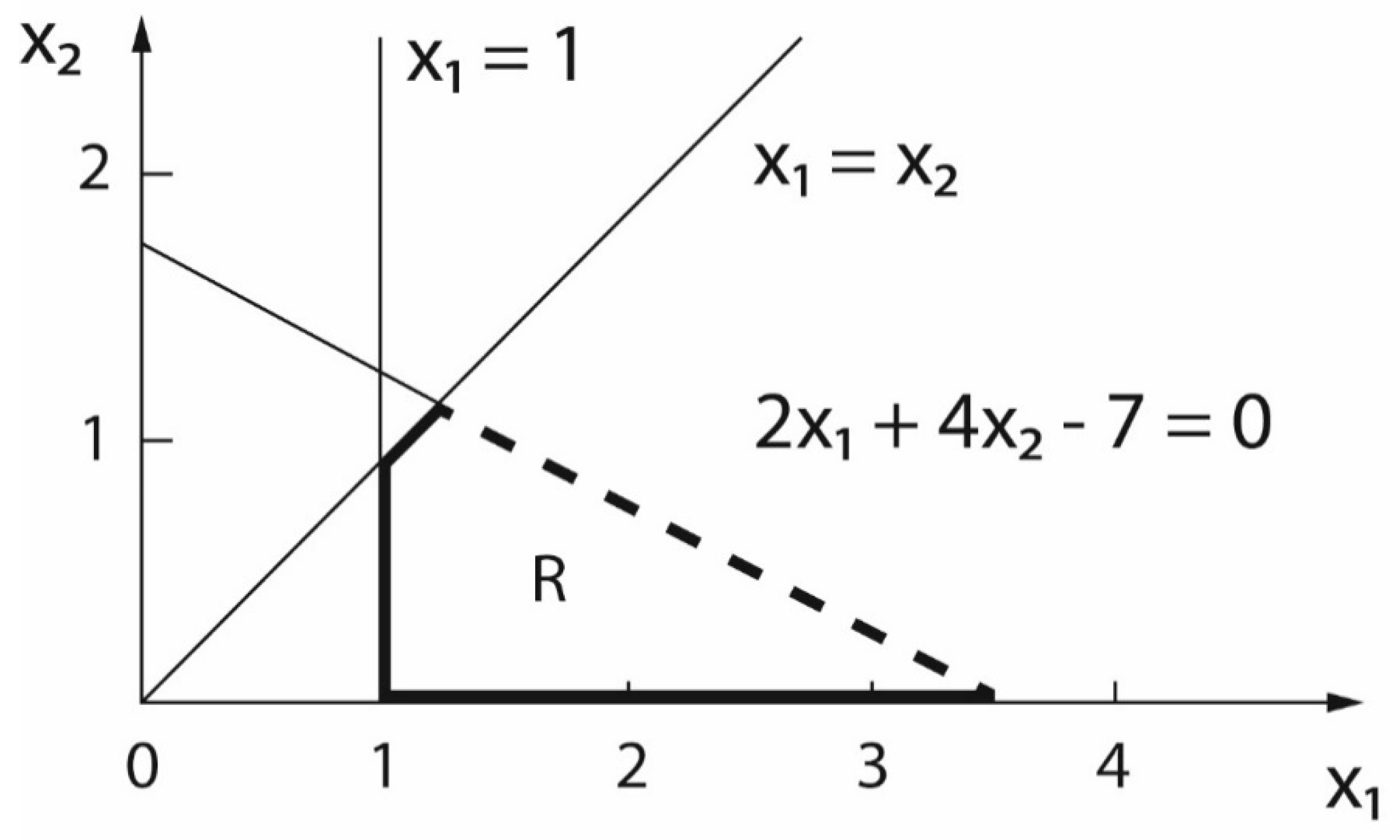
If a_X = 1, then f_X(1) < f_X(2). This inequality is equivalent to −2x₁ + 1 < −4(x₁ + x₂) + 8 or 2x₁ + 4x₂ < 7 or 2x₁ + 4x₂ − 7 < 0.

Taken the constraints x₁ ≥ 1 and x₁ ≥ x₂ into account yields the following area (see Figure 1) in which a_X = 1. This is the area R situated within the polygon with vertices (1,0), (1,1), (7/6,7/6), (7/2,0), where points on the line 2x₁ + 4x₂ − 7 = 0 are excluded. We note that for all points in this area, h_X = 1.

When it comes to arrays X for which a_X = 1, this set consists of all decreasing convergent arrays with (x₁,x₂) in the area R.

3.2. The Generalized Discrete h- and g-Index

We next show that a_X exists for each converging and decreasing X in (R⁺)^∞. For this, we recall the definitions of the generalized discrete h- and g-index [11].

Definition 4.

The generalized discrete h- and g-index [11]:

Given X, a decreasing array in (R⁺)^∞. Let θ > 0, then

(1) 

z = h_θ(X), in short h_θ, iff z is the largest index such that x_z ≥ θz; if such an index does not exist, namely when x₁ < θ, then we define z = h_θ(X) = 0;

(2) 

z = g_θ(X), in short g_θ, iff z is the largest index such that${\displaystyle \sum }_{i=1}^z{x}_i$≥ θz²$\iff \frac{1}{z} {\displaystyle \sum }_{i=1}^z{x}_i\ge \theta z$; if such an index does not exist, e.g., when${\displaystyle \sum }_{i=1}^{\propto }{x}_i<\theta$, then we define z = g_θ(X) = 0.

We note that if a and b are natural numbers and X = ${\left({\mathrm{x}}_{\mathrm{r}}\right)}_{\mathrm{r}=1,2\dots }$ is a decreasing array in (R⁺)^∞, then the property for r ≤ a: ${\displaystyle \sum }_{\mathrm{i}=1}^{\mathrm{r}}{\mathrm{x}}_{\mathrm{i}}\ge {\mathsf{\theta }\mathrm{a}}^2$ implies that g_θ(X) ≥ a; similarly, the property for r > b: ${\displaystyle \sum }_{\mathrm{i}=1}^{\mathrm{r}}{\mathrm{x}}_{\mathrm{i}}<{\mathsf{\theta }\mathrm{b}}^2$ implies g_θ(X) ≤ b.

We finally also define the discrete f-index, already introduced in [10], for the continuous case.

(3) 

z = f_θ(X), in short f_θ, if z is the largest index such that$\frac{1}{2}\left(x_z+\frac{1}{z} {\displaystyle \sum }_{i=1}^z{x}_i\right)\ge \theta z$. Again, if such an index does not exist, we define z = f_θ(X) = 0.

In [10], we found that in the continuous case, the solution of our problem was obtained as f_(3/4)(X) (where f is the continuous analog of the discrete f-index introduced above). We will show further on that this is not the case for the discrete case studied here.

Proposition 1.

The indicators h_θ(X), g_θ(X), and f_θ(X) are each decreasing in θ.

Proof of Proposition 1.

Let θ₁ > θ₂. If ${\mathrm{z}}_1={\mathrm{h}}_{{\mathsf{\theta }}_1}$(X) and ${\mathrm{z}}_2={\mathrm{h}}_{{\mathsf{\theta }}_2}$(X), then ${\mathrm{x}}_{{\mathrm{z}}_1}\ge {\mathsf{\theta }}_1{\mathrm{z}}_1>{\mathsf{\theta }}_2{\mathrm{z}}_1$. As ${\mathrm{z}}_2$ is the largest index such that ${\mathrm{x}}_{{\mathrm{z}}_2}>{\mathsf{\theta }}_2{\mathrm{z}}_2$, it follows that ${\mathrm{z}}_1={\mathrm{h}}_{{\mathsf{\theta }}_1}$(X) ≤ ${\mathrm{z}}_2={\mathrm{h}}_{{\mathsf{\theta }}_2}$(X). Consequently, θ₁ > θ₂ implies ${\mathrm{h}}_{{\mathsf{\theta }}_1}$(X) ≤ ${\mathrm{h}}_{{\mathsf{\theta }}_2}$(X), showing that h_θ(X) is decreasing in θ.

Similarly, if θ₁ > θ₂, $z_1=g_{{\theta }_1}$(X), and $z_2=g_{{\theta }_2}$(X), then $\frac{1}{z_1} {\displaystyle \sum }_{i=1}^{z_1}{x}_i\ge {\theta }_1 z_1>{\theta }_2 z_1$. As $z_2$ is the largest index such that $\frac{1}{z_2} {\displaystyle \sum }_{i=1}^{z_2}{x}_i>{\theta }_2{z}_2$, it follows, like in the case for the generalized discrete h-index, that g_θ(X) is decreasing in θ. Finally, it also follows that f_θ(X) is decreasing in θ. □

Theorem 1.

For all X, decreasing in (R⁺)^∞ and all θ > 0, h_θ(X) ≤ f_θ(X) ≤ g_θ(X). Hence, f_θ(X)$\in$[[h_θ(X), g_θ(X)]].

Proof of Theorem 1.

Let a = f_θ(X), then, by the definition of f_θ(X),

$$\frac{1}{2}\left({\mathrm{x}}_{\mathrm{a}+1}+{\mathrm{x}}_{\mathrm{a}+1}\right)\le \frac{1}{2}\left({\mathrm{x}}_{\mathrm{a}+1}+\frac{1}{\mathrm{a}+1}{\displaystyle \sum }_{\mathrm{i}=1}^{\mathrm{a}+1}{\mathrm{x}}_{\mathrm{i}}\right)<\mathsf{\theta }\left(\mathrm{a}+1\right)$$

Hence, ${\mathrm{x}}_{\mathrm{a}+1}<\mathsf{\theta }\left(\mathrm{a}+1\right)$ and thus a+1 > h_θ(X), leading to a = f_θ(X) ≥ h_θ(X). Now, for a = f_θ(X), we further have $\frac{1}{\mathrm{a}}{\displaystyle \sum }_{\mathrm{i}=1}^{\mathrm{a}}{\mathrm{x}}_{\mathrm{i}}\ge \frac{1}{2}\left({\mathrm{x}}_{\mathrm{a}}+\frac{1}{\mathrm{a}}{\displaystyle \sum }_{\mathrm{i}=1}^{\mathrm{a}}{\mathrm{x}}_{\mathrm{i}}\right)\ge \mathsf{\theta }\mathrm{a}$, hence a ≤ g_θ(X). This proves Theorem 1.  □

3.3. Excluding the Theoretical Case of Infinitely Many Minima

Next, we need two lemmas.

Lemma 1.

If X is decreasing, then$\stackrel{=}{X}$with${\left(\stackrel{=}{X}\right)}_i=\frac{1}{i}{\displaystyle \sum }_{j=1}^i{x}_j$is also decreasing. This decrease is strict if x₁ > x₂.

Proof of Lemma 1.

The easy proof is left to the reader. □

As for given X and n > 0, x_n = θn, for $\theta =\frac{x_n}{n}$, it is clear that $\left\{h_{\theta }\left(X\right), \theta >0\right\}=N$ (where n = 0 is reached for θ > x₁). Now, we prove a similar result for g_θ(X).

Lemma 2.

For given X, decreasing and convergent, $\left\{g_{\theta }\left(X\right), \theta >0\right\}=\mathit{N}$

Proof of Lemma 2.

It is clear that $\left\{g_{\theta }\left(X\right), \theta >0\right\}$ $\subset$ N (recall that g_θ(X) = 0 if $\theta >{\displaystyle \sum }_{j=1}^{\infty }{x}_j$). Next, we consider the opposite relation.

The value n = 0 results from all θ > ${\displaystyle \sum }_{j=1}^{\infty }{x}_j$. If n ≠ 0, we define $\theta =\frac{1}{n^2}{\displaystyle \sum }_{j=1}^n{x}_j>0$. Then, we have, using Lemma 1, for all i ≤ n, $\frac{1}{i}{\displaystyle \sum }_{j=1}^i{x}_j\ge \frac{1}{n}{\displaystyle \sum }_{j=1}^n{x}_j$ = θn. Consequently,

$${\displaystyle \sum }_{j=1}^i{x}_j\ge \theta ni\ge \theta i^2$$

(3)

Now, for all i > n, using Lemma 1 again, $\frac{1}{i}{\displaystyle \sum }_{j=1}^i{x}_j \le \frac{1}{n}{\displaystyle \sum }_{j=1}^n{x}_j=\mathsf{\theta } \mathrm{n}< \mathsf{\theta }\mathrm{i}$ and hence

$${\displaystyle \sum }_{j=1}^i{x}_j<\mathsf{\theta } i^2$$

(4)

It follows from (3) and (4) and the definition of g_θ that n = g_θ. This shows that $\left\{g_{\theta }\left(X\right), \theta >0\right\}=N.$ □

Theorem 2.

Given X is decreasing and convergent and a > g_(0.5)(X), then f_X(x) is strictly increasing for x > a.

Proof of Theorem 2.

From Lemma 2, it follows that there exists θ₀ < 0.5 such that $a=g_{{\theta }_0}\left(X\right)$. Indeed, g_θ(X) is a decreasing function of θ and a > g_(0.5)(X). Hence

${\displaystyle \sum }_{i=1}^a{x}_i\ge {\theta }_0{a}^2$ and ${\displaystyle \sum }_{i=1}^{a+1}{x}_i<{\theta }_0{\left(a+1\right)}^2$. From this inequality, we derive that $a^3-2a{\displaystyle \sum }_{i=1}^a{x}_i\le a^3-2a{\theta }_0{a}^2=a^3\left(1-2{\theta }_0\right)$ and ${\left(a+1\right)}^3-2\left(a+1\right){\displaystyle \sum }_{i=1}^{a+1}{x}_i>{\left(a+1\right)}^3-2\left(a+1\right){\theta }_0{\left(a+1\right)}^2={\left(a+1\right)}^3\left(1-2{\theta }_0\right)$. Consequently, ${\left(a+1\right)}^3-2\left(a+1\right){\displaystyle \sum }_{i=1}^{a+1}{x}_i>a^3-2a{\displaystyle \sum }_{i=1}^a{x}_i,$ which shows that f_X(x) is strictly increasing for x > g_(0.5)(X). □

It follows from Theorem 2 that if a_X exists, it belongs to [[1, g_(0.5)(X)]], which excludes the theoretical case of infinitely many minima.

3.4. Excluding the Case of More Than One Minimum

Next, to exclude the case of a local maximum, following a first local minimum, we continue as follows.

Theorem 3.

For all X, decreasing and convergent in (R⁺)^∞ and for all a$\in {\mathit{N}}_{\mathbf{0}},$we have the following property:

f_X(a + 1) > f_X(a) implies that f_X(a + 2) > f_X(a + 1).

Proof of Theorem 3.

$$\begin{gathered} \mathrm{f}\mathrm{x}\left(a+1\right)>\mathrm{f}\mathrm{x}\left(a\right) \\ \iff {\displaystyle \sum }_{i=1}^{\infty }{x}_i^2-2\left(a+1\right)\left({\displaystyle \sum }_{i=1}^{a+1}{x}_i\right)+{\left(a+1\right)}^3>{\displaystyle \sum }_{i=1}^{\infty }{x}_i^2-2a\left({\displaystyle \sum }_{i=1}^a{x}_i\right)+a^3 \\ \iff 2\left(a+1\right)\left({\displaystyle \sum }_{i=1}^{a+1}{x}_i\right)-2a \left({\displaystyle \sum }_{i=1}^{a+1}{x}_i-x_{a+1}\right)<{\left(a+1\right)}^3-a^3=3a^2+3a+1 \\ \iff 2\left({\displaystyle \sum }_{i=1}^{a+1}{x}_i\right)+2a{x}_{a+1}<3a^2+3a+1 \end{gathered}$$

(5)

From (5), we also note that (2(a+1)+2a)x_a+1 = (4a+2) x_a+1 < $3a^2+3a+1$, or x_a+1 < a+1.

Now, we have to show that

$$\begin{gathered} \mathrm{f}\mathrm{x}\left(a+2\right)>\mathrm{f}\mathrm{x}\left(a+1\right) \\ \iff {\displaystyle \sum }_{i=1}^{\infty }{x}_i^2-2\left(a+2\right)\left({\displaystyle \sum }_{i=1}^{a+2}{x}_i\right)+{\left(a+2\right)}^3>{\displaystyle \sum }_{i=1}^{\infty }{x}_i^2-2\left(a+1\right)\left({\displaystyle \sum }_{i=1}^{a+1}{x}_i\right)+{\left(a+1\right)}^3 \\ \iff 2\left(\left(a+2\right)\left({\displaystyle \sum }_{i=1}^{a+2}{x}_i\right)-\left(a+1\right)\left({\displaystyle \sum }_{i=1}^{a+1}{x}_i\right)\right)<{(a+2)}^3-{\left(a+1\right)}^3=3a^2+9a+7 \\ \iff 2\left(\left(a+2\right)\left({\displaystyle \sum }_{i=1}^{a+1}{x}_i+x_{a+2}\right)-\left(a+1\right)\left({\displaystyle \sum }_{i=1}^{a+1}{x}_i\right)\right)<3a^2+9a+7 \\ \iff 2\left({\displaystyle \sum }_{i=1}^{a+1}{x}_i\right)+2\left(a+2\right)x_{a+2}<3a^2+9a+7 \end{gathered}$$

We rewrite the left-hand side of this inequality as

$$\left(2{\displaystyle \sum }_{i=1}^{a+1}{x}_i+2a{x}_{a+1}\right)-2a{x}_{a+1}+4x_{a+2}+2a{x}_{a+2}$$

Because of (5), we know that this expression is smaller than

$$\left(3a^2+3a+1\right)+\left(2a{x}_{a+2}-2a{x}_{a+1}\right)+4x_{a+2}$$

(6)

As X is decreasing and hence 2ax_a+1 ≥ 2ax_a+2, the expression (6) is smaller than or equal to

$$\left(3a^2+3a+1\right)+4x_{a+1}$$

(7)

Finally, because the note after inequality (5), expression (7) is smaller than

$$\left(3a^2+3a+1\right)+4\left(a+1\right)=3a^2+7a+5$$

(8)

Finally, we see that

$$3a^2+7a+5<3a^2+9a+7$$

(9)

which proves this theorem. □

Theorem 3 shows that a minimum for f_X(x) exists and that a_X is uniquely defined. We note, however, that the minimum of f_X is not always unique. Indeed, the following example gives a case where there are two minima.

Let X = (5, 4.5). Then, f_X(1) = 45.25 − 10 + 1 = 36.25; f_X(2) = 45.25 − 38 + 8 = 15.25; f_X(3) = 45.25 − 57 + 27 = 15.25; f_X(4) = 45.25 − 76 + 64 = 33.25. Hence, a_X = 3.

From the previous proof, we know that f_X(a+1) > f_X(a) implies x_a+1 < a + 1. Hence, a + 1 > h(X). Hence, f_X(a) is decreasing on [[1, …, h(X)]]. The next proposition shows that this is actually a strict decrease.

Proposition 2.

If h(X) > 1, then f_X(a) is strictly decreasing for a in [[1, …, h(X)]].

Note that the requirement h(X) > 1 implies that a_X > 1.

Proof of Proposition 2.

For any natural number a, such that a+1 ≤ h(X), we have x₁ ≥ …x_a ≥ x_a+1 ≥ a + 1. Consequently, for all j = 1, …, a + 1, x_j − a − 1 ≥ 0.

Hence, (x_j − a) > (x_j − a − 1) ≥ 0 and thus (x_j − a)² > (x_j − a − 1)².

Now, f_X(a+1) $={\displaystyle \sum }_{i=1}^{a+1}{\left(x_i-a-1\right)}^2+{\displaystyle \sum }_{i=a+2}^{\infty }{x}_i^2$ < ${\displaystyle \sum }_{i=1}^{a+1}{\left(x_i-a\right)}^2+{\displaystyle \sum }_{i=a+2}^{\infty }{x}_i^2$ = ${\displaystyle \sum }_{i=1}^a{\left(x_i-a\right)}^2+{\left(x_{a+1}-a\right)}^2+{\displaystyle \sum }_{i=a+1}^{\infty }{x}_i^2-x_{a+1}^2<{\displaystyle \sum }_{i=1}^a{\left(x_i-a\right)}^2+{\displaystyle \sum }_{i=a+1}^{\infty }{x}_i^2$ = f_X(a). Indeed, (x_a+1 − a)² − (x_a+1)² = −2ax_a+1 + a² = a(a – 2x_a+1) < 0, as 2x_a+1 ≥ x_a+1 ≥ a + 1 > a. □

As h(X) ≤ g(X) ≤ g_(0.5)(X), this result shows that $a_X\in ⟦h\left(X\right), g_{\left(0.5\right)}\left(X\right)⟧$.

We next reformulate inequality (2), leading to a refinement of the previous observation.

Theorem 4.

Given an array X, converging and decreasing in(R⁺)^∞, then a_X (≠1) is characterized as the largest natural number that satisfies the following inequality:

$$x_{a_X}+\frac{1}{a_X-1}{\displaystyle \sum }_{i=1}^{a_X}{x}_i\ge \frac{3a_X}{2}+\frac{1}{2\left(a_X-1\right)}$$

Proof of Theorem 4.

From Equations (1) and (2), we have

$$\begin{gathered} -2({\mathrm{a}}_{\mathrm{X}}-1)({{\displaystyle \sum }}_{i=1}^{a_X-1}{x}_i)+{({\mathrm{a}}_{\mathrm{X}}-1)}^3\ge -2{\mathrm{a}}_{\mathrm{X}}({{\displaystyle \sum }}_{i=1}^{a_X}{x}_i){{\mathrm{a}}_{\mathrm{X}}}^3 \\ <=>-2({\mathrm{a}}_{\mathrm{X}}-1)({{\displaystyle \sum }}_{i=1}^{a_X-1}{x}_i)+{({\mathrm{a}}_{\mathrm{X}}-1)}^3\ge -2({\mathrm{a}}_{\mathrm{X}}-1)({{\displaystyle \sum }}_{i=1}^{a_X-1}{x}_i)-2({{\displaystyle \sum }}_{i=1}^{a_X}{x}_i)-2({\mathrm{a}}_{\mathrm{X}}-1){\mathrm{a}}_{\mathrm{X}}+{{\mathrm{a}}_{\mathrm{X}}}^3 \\ <=>{({\mathrm{a}}_{\mathrm{X}}-1)}^3)\ge -2({{\displaystyle \sum }}_{i=1}^{a_X}{x}_i)-2({\mathrm{a}}_{\mathrm{X}}-1)a_X+{{\mathrm{a}}_{\mathrm{X}}}^3 \\ <=>2({{\displaystyle \sum }}_{i=1}^{a_X}{x}_i)+2({\mathrm{a}}_{\mathrm{X}}-1)X_a\ge 3{\mathrm{a}}_{\mathrm{X}}({\mathrm{a}}_{\mathrm{X}}-1)+1 \\ <=>x_{a_X}+\frac{1}{a_X-1}{{\displaystyle \sum }}_{i=1}^{a_X}{x}_i\ge \frac{3a_X}{2}+\frac{1}{2\left(a_X-1\right)} \end{gathered}$$

 □

Theorem 5.

If f_(3/4)(X) > 1, then, f_(3/4)(X) ≤ a_X and hence $a_X\in ⟦f_{\left(\frac{3}{4}\right)}\left(X\right), g_{\left(0.5\right)}\left(X\right)⟧$.

Proof of Theorem 5.

If a = f_(3/4)(X), then

$$\frac{1}{2}\left(x_a+\frac{1}{a-1}{{\displaystyle \sum }}_{i=1}^a{x}_i\right)=\frac{x_a}{2}+\frac{1}{2a}{{\displaystyle \sum }}_{i=1}^a{x}_i+\left(\frac{1}{2\left(a-1\right)}-\frac{1}{2a}\right){{\displaystyle \sum }}_{i=1}^a{x}_i\ge \frac{3a}{4}+\frac{1}{2}\frac{1}{a\left(a-1\right)}{{\displaystyle \sum }}_{i=1}^a{x}_i.$$

(10)

As a = f_(3/4)(X) ≤ g_(3/4)(X), we have $\frac{1}{a}{\displaystyle \sum }_{i=1}^a{x}_i\ge \frac{3a}{4}$.

Consequently, by Theorem 4, we find that

(10) ≥$\frac{3a}{4}+\frac{1}{2\left(a-1\right)}\frac{3a}{4}\ge \frac{3a}{4}+\frac{3}{8\left(a-1\right)}>\frac{3a}{4}+\frac{1}{4\left(a-1\right)}$.

As a_X is the largest natural number with this property, this ends the proof of Theorem 5. □

3.5. Examples

Example 1.

We provide an example such that the following strict inequalities hold: h_(3/4)(X) < f_(3/4)(X) < a_X < g_(0.5)(X).

Let X = (6,1,1). Then, h_(3/4)(X) = 1 < f_(3/4)(X) = 2 < a_X = 3 < g_(0.5)(X) = 4.

This example shows that, contrary to the continuous case, f_(3/4)(X) is not always the solution of the minimization problem. Stated otherwise, in general, f_(3/4)(X) ≠ a_X. Yet, one may say that f_(3/4)(X) is a (close) under limit.

As g_(3/4)(X) ≥ f_(3/4)(X), it was an upper limit for a_X in the continuous case. One may wonder if, in the discrete case, g_(3/4)(X) is either an under or an upper limit for a_X. Yet, none of these two alternatives are correct. In the case of X = (6,1,1), g_(3/4)(X) = 3 = a_X. However, for X = (8,1), h_(3/4)(X) = 1 < f_(3/4)(X) = 2 = a_X < g_(3/4)(X) = 3 < g_(0.5)(X) = 4, while for X = (2, 0.9), h_(3/4)(X) = 1 = f_(3/4)(X) = g_(3/4)(X) < a_X = g_(0.5)(X) = 2.

We already observed that g_(3/4)(X) can be smaller than, equal to, and larger than a_X. We next show that a_X ≤ g_(3/4)(X) +1.

Proposition 3.

Given an array X, converging and decreasing in (R⁺)^∞, then a_X ≤ g_(3/4)(X) +1.

Proof of Proposition 3.

We show that if a = g_(3/4)(X) +1, then f_X(a+1) > f_X(a). This inequality is equivalent to

$$\begin{gathered} -2\left(a+1\right)\left({\displaystyle \sum }_{i=1}^{a+1}{x}_i\right)+{\left(a+1\right)}^3>-2a\left({\displaystyle \sum }_{i=1}^a{x}_i\right)+a^3 \\ \iff -2a{x}_{a+1}-2\left({\displaystyle \sum }_{i=1}^{a+1}{x}_i\right)+{\left(a+1\right)}^3>a^3 \\ \iff a{x}_{a+1}+\left({\displaystyle \sum }_{i=1}^{a+1}{x}_i\right)<\frac{1}{2}\left(3a^2+3a+1\right)=\frac{3}{2}a\left(a+1\right)+\frac{1}{2} \end{gathered}$$

Now, a = g_(3/4)(X) +1 > g_(3/4)(X) ≥ h_(3/4)(X) and hence x_a+1 ≤ x_a < (3/4)a.

Moreover, ${\displaystyle \sum }_{i=1}^{a+1}{x}_i={\displaystyle \sum }_{i=1}^a{x}_i+x_{a+1}\le {\displaystyle \sum }_{i=1}^a{x}_i+x_a<\frac{3}{4}{a}^2+\frac{3}{4}a$.

Consequently, $a{x}_{a+1}+\left({\displaystyle \sum }_{i=1}^{a+1}{x}_i\right)<\frac{3}{4}{a}^2+\frac{3}{4}{a}^2+\frac{3}{4}a=\frac{3}{2}{a}^2+\frac{3}{4}a<\frac{3}{2}a\left(a+1\right)+\frac{1}{2}$, which proves Proposition 3. □

Example 2.

If X = (2,2,2), then a_X = 3 and g_(3/4)(X) = 2, providing an example where there is an equality for the expression a_X ≤ g_(3/4)(X) +1.

3.6. An Upper Bound for a_X

We already know that g_(3/4)(X) is not an upper bound for a_X and that g_(0.5)(X) is. Hence, we wonder if there a number strictly between 0.5 and 0.75 that leads to an upper bound for all X.

Theorem 6.

An upper bound for a_X is provided by g_(7/12)(X).

Proof of Theorem 6.

Take a ≥ g_s(X), with s being any real number strictly smaller than 0.75.

Hence, a+1 > g_s(X) ≥ h_s(X). From these inequalities, we derive

$$\{\begin{array}{c}{x}_{a+1}<s\left(a+1\right)\\ {\displaystyle {\displaystyle \sum }_{i=1}^{a+1}}{x}_i<s{\left(a+1\right)}^2\end{array}$$

Multiplying the first inequality by a and adding the two resulting inequalities yields

$$a{x}_{a+1}+{\displaystyle \sum }_{i=1}^{a+1}{x}_i<sa\left(a+1\right)+s{\left(a+1\right)}^2$$

Now, from Proposition 3, we know that f_X(a+1) > f_X(a), hence a ≥ a_X if

$$a{x}_{a+1}+\left({\displaystyle \sum }_{i=1}^{a+1}{x}_i\right)\le \frac{3}{2}a\left(a+1\right)+\frac{1}{2}$$

From this inequality, we find that s must satisfy the following inequality:

$$sa\left(a+1\right)+s{\left(a+1\right)}^2=s \left(2a^2+3a+1\right)\le \frac{1}{2}\left(3a^2+3a+1\right)$$

leading to

$$s\le \frac{3a^2+3a+1}{2\left(2a^2+3a+1\right)}$$

(11)

This inequality must hold for any natural number a different from zero. As the right-hand side is increasing in a, we consider the inequality for a = 1, leading to s ≤ 7/12. □

Corollary 1.

Given an array X, converging and decreasing in (R⁺)^∞, then $a_X\in ⟦f_{\left(\frac{3}{4}\right)}\left(X\right), g_{\left(\frac{7}{12}\right)}\left(X\right)⟧$.

We already observed that if a_X = 1, then h(X) = 1. What about the converse? The next proposition answers this question.

Proposition 4.

If h(X) = 1, then a_x can be larger than any natural number b.

Proof of Proposition 4.

Consider X = (z, 1, 0, …) and we want to find z such that a_X ≥ b. If a_X ≥ b, then f_X(b) ≥ f_X(b + 1), or (with b > 2): 2(z + 1) ≥ 3b² + 3b + 1. Hence, it suffices to take z > (3b² + 3b − 1)/2. □

An example: Suppose that we want a_X ≥ 18. Taking z = 512 leads to X = (512, 1, 0, …) and a_X = 18. If, however, we want a_X ≥ 19, then z = 570, leading to X = (570, 1, 0, …) with a_X = 20.

4. Applications

First, we give a new characterization of the classical h-index [1], i.e., the case θ = 1.

Proposition 5.

Given X decreasing and convergent, then h(X) = max{a$\in$N; A_a ≤ X}.

Proof of Proposition 5.

Writing h(X) simply as h, we see that A_h ≤ X because for A_h and j ≤ h, x_j ≥ h, while for all j > h, x_j ≥ 0. This shows that h ≤ max{a $\in$ N; A_a ≤ X}.

Now, let a_m = max{a $\in$ N; A_a ≤ X}. Then, we see that for all j ≤ a_m, x_j ≥ a_m, while for all j > a_m, x_j ≥ 0. As h is defined as the largest number with this property, we see that h ≥ a_m = max{a $\in$ N; A_a ≤ X}. This proves this proposition. □

Before continuing with the next proposition, we recall the definition of the majorization partial order for finite sequences.

Definition 5.

The majorization order [12]:

Let X, Y $\in$ (R⁺)^k, where k is any finite number in N₀ = {1, 2, 3, … }. The array X is majorized by Y, or X is smaller than or equal to Y in the majorization order, denoted as X -< Y if for all i = 1,…,N:

$$\{\begin{array}{c}{\displaystyle {\displaystyle \sum }_{i=1}^N}{x}_i={\displaystyle {\displaystyle \sum }_{i=1}^N}{y}_i and \\ {\displaystyle {\displaystyle \sum }_{j=1}^i}{x}_j\le {\displaystyle {\displaystyle \sum }_{j=1}^i}{y}_j; \forall i=1,\dots ,N.\end{array}$$

Proposition 6.

If X is finite with length N and $\frac{1}{N}{\displaystyle \sum }_{j=1}^N{x}_j$ = $\overline{x}$ is a natural number, then A_a -< X $\iff$ a = $\overline{x}$, where -< denotes the majorization partial order.

Proof of Proposition 6.

If A_a -< X, then, for all j = 1, …, N, $ja\le {\displaystyle \sum }_{k=1}^j{x}_k$ and Na = ${\displaystyle \sum }_{k=1}^N{x}_k$. Consequently, a = $\overline{x}$.

Conversely, if a = $\overline{x}$ (and hence $\overline{x}$ must be a natural number), we have

$$A_a=\left(\underset{\overline{x} times}{\underbrace{\overline{x},\overline{x},\dots ,\overline{x}}, 0,0, \dots }\right)$$

and hence for all j ≤ N, $j\overline{x}\le {\displaystyle \sum }_{k=1}^j{x}_k$ and for j = N, $N\overline{x}={\displaystyle \sum }_{k=1}^N{x}_k$. This shows that A_a -< X. □

Finally, we show that a_X is increasing in X.

Theorem 7.

If X < Y, then a_X ≤ a_Y.

Proof of Theorem 7.

We know that a_X is the largest index such that

$$\begin{gathered} {\displaystyle \sum }_{i=1}^{\infty }{x}_i^2-2\left(a_X-1\right)\left({\displaystyle \sum }_{i=1}^{a_X-1}{x}_i\right)+{\left(a_X-1\right)}^3\ge {\displaystyle \sum }_{i=1}^{\infty }{x}_i^2-2a_X\left({\displaystyle \sum }_{i=1}^{a_X}{x}_i\right)+{\left(a_X\right)}^3 \\ \iff 2\left({\displaystyle \sum }_{i=1}^{a_X-1}{x}_i\right)+{\left(a_X-1\right)}^3\ge -2a_X{x}_{a_X}+{\left(a_X\right)}^3 \end{gathered}$$

Now, we also know that for all i ≥ 1, y_i ≥ x_i. Hence, $\left({\displaystyle \sum }_{i=1}^{a_X-1}{y}_i\right)\ge \left({\displaystyle \sum }_{i=1}^{a_X-1}{x}_i\right)$ and $-2a_X{y}_{a_X}\le -2a_X{x}_{a_X}$. This leads to

$$2\left({\displaystyle \sum }_{i=1}^{a_X-1}{y}_i\right)+{\left(a_X-1\right)}^3\ge -2a_X{y}_{a_X}+{\left(a_X\right)}^3$$

Hence, also

$${\displaystyle \sum }_{i=1}^{\infty }{y}_i^2-2a_X\left({\displaystyle \sum }_{i=1}^{a_X-1}{y}_i\right)+2\left({\displaystyle \sum }_{i=1}^{a_X-1}{y}_i\right)+{\left(a_X-1\right)}^3\ge {\displaystyle \sum }_{i=1}^{\infty }{y}_i^2-2a_X\left({\displaystyle \sum }_{i=1}^{a_X}{y}_i\right)+{\left(a_X\right)}^3$$

This can be written as

$${\displaystyle \sum }_{i=1}^{\infty }{y}_i^2-2\left(a_X-1\right)\left({\displaystyle \sum }_{i=1}^{a_X-1}{y}_i\right)+{\left(a_X-1\right)}^3\ge {\displaystyle \sum }_{i=1}^{\infty }{y}_i^2-2a_X\left({\displaystyle \sum }_{i=1}^{a_X}{y}_i\right)+{\left(a_X\right)}^3$$

(12)

As a_Y is the largest index with property (12), this shows that a_X ≤ a_Y. □

Remark 2.

If X < Y (strict), then it is possible that a_X = a_Y. An example is given by X = (6,1,1) < Y = (6,2,1), for which a_X = a_Y = 3.

5. Conclusions

In this article, we studied the following problem:

Given a converging decreasing array X in (R⁺)^∞, find the largest natural number a such that the Euclidean distance d(X,A_a) is minimal.

We have shown that this problem has a solution, which is always situated in the interval $⟦h_{\left(\frac{3}{4}\right)}\left(X\right), g_{\left(\frac{7}{12}\right)}\left(X\right)⟧$. Yet, the solution is not necessarily unique. It was shown that a discrete and an analogous continuous problem have related but not the same solutions. Our contribution illustrates how a formalism derived in the context of research evaluation and informetrics [1] can be used to solve a purely mathematical problem.

References

- Hirsch, J.E. An index to quantify an individual’s scientific research output. Proc. Natl. Acad. Sci. USA 2005, 102, 16569–16572. [Google Scholar] [CrossRef] [PubMed] [Green Version]
- Bouyssou, D.; Marchant, T. Ranking scientists and departments in a consistent manner. J. Am. Soc. Inf. Sci. Technol. 2011, 62, 1761–1769. [Google Scholar] [CrossRef] [Green Version]
- Waltman, L.; van Eck, N.J. The inconsistency of the h-index. J. Am. Soc. Inf. Sci. Technol. 2012, 63, 406–415. [Google Scholar] [CrossRef]
- Egghe, L. Theory and practise of the g-index. Scientometrics 2006, 69, 131–152. [Google Scholar] [CrossRef]
- Alonso, S.; Cabrerizo, F.J.; Herrera-Viedma, E.; Herrera, F. H-index: A review focused in its variants, computation and standardization for different scientific fields. J. Informetr. 2009, 3, 273–289. [Google Scholar] [CrossRef] [Green Version]
- Egghe, L. The Hirsch-index and related impact measures. Annu. Rev. Inf. Sci. Technol. 2010, 44, 65–114. [Google Scholar] [CrossRef]
- Rousseau, R.; Egghe, L.; Guns, R. Becoming Metric-Wise: A Bibliometric Guide for Researchers; Chandos: Oxford, UK, 2018. [Google Scholar]
- Egghe, L.; Rousseau, R. Polar coordinates and generalized h-type indices. J. Informetr. 2020, 14, 101024. [Google Scholar] [CrossRef]
- Egghe, L.; Rousseau, R. Infinite sequences and their h-type indices. J. Informetr. 2019, 13, 291–298. [Google Scholar] [CrossRef]
- Egghe, L.; Rousseau, R. Solution by step functions of a minimum problem in L2 [0,T], using generalized h- and g-indices. J. Informetr. 2019, 13, 785–792. [Google Scholar] [CrossRef]
- van Eck, N.J.; Waltman, L. Generalizing the h-and g-indices. J. Informetr. 2008, 2, 263–271. [Google Scholar] [CrossRef] [Green Version]
- Hardy, G.H.; Littlewood, G.E.; Pólya, G. Inequalities; Cambridge University Press: Cambridge, UK, 1934. [Google Scholar]
Figure 1.
Zone R in (x1,x2)-plane where aX = 1.
© 2020 by the authors. Licensee MDPI, Basel, Switzerland. This article is an open access article distributed under the terms and conditions of the Creative Commons Attribution (CC BY) license (http://creativecommons.org/licenses/by/4.0/).
Share and Cite
MDPI and ACS Style
Egghe, L.; Rousseau, R. Minimal Impact One-Dimensional Arrays. Mathematics 2020, 8, 811. https://doi.org/10.3390/math8050811
AMA Style
Egghe L, Rousseau R. Minimal Impact One-Dimensional Arrays. Mathematics. 2020; 8(5):811. https://doi.org/10.3390/math8050811
Chicago/Turabian StyleEgghe, Leo, and Ronald Rousseau. 2020. "Minimal Impact One-Dimensional Arrays" Mathematics 8, no. 5: 811. https://doi.org/10.3390/math8050811
Note that from the first issue of 2016, this journal uses article numbers instead of page numbers. See further details here.