Numerical Results for Linear Sequential Caputo Fractional Boundary Value Problems

1
Department of Mathematics, Dixie State University, St. George, UT 84770, USA
2
Department of Mathematics, University of Louisiana at Lafayette, Lafayette, LA 70504, USA
*
Author to whom correspondence should be addressed.
†
These authors contributed equally to this work.
Mathematics 2019, 7(10), 910; https://doi.org/10.3390/math7100910
Submission received: 17 July 2019
/
Revised: 26 September 2019
/
Accepted: 27 September 2019
/
Published: 1 October 2019
Abstract
:The generalized monotone iterative technique for sequential order Caputo fractional boundary value problems, which is sequential of order q, with mixed boundary conditions have been developed in our earlier paper. We used Green’s function representation form to obtain the linear iterates as well as the existence of the solution of the nonlinear problem. In this work, the numerical simulations for a linear nonhomogeneous sequential Caputo fractional boundary value problem for a few specific nonhomogeneous terms with mixed boundary conditions have been developed. This in turn will be used as a tool to develop the accurate numerical code for the linear nonhomogeneous sequential Caputo fractional boundary value problem for any nonhomogeneous terms with mixed boundary conditions. This numerical result will be essential to solving a nonlinear sequential boundary value problem, which arises from applications of the generalized monotone method.
1. Introduction
It is known that in [1] the half order fractional diffusion model has been established to be useful and also economical. For some more applications in elasticity, continuum mechanics, and some qualitative study of those models see [2,3,4,5,6,7,8,9,10,11,12,13,14,15,16,17,18,19,20,21,22,23,24,25,26,27] for initial and boundary value problems. However, when we need to compare our model with the integer model, our fractional boundary value problem should yield the integer model as a special case. This in general is not true even though the initial and boundary conditions and the basis solution for the fractional order is when See [28,29,30]. In short, the integer result of well known second order results will not be a special case of a order when . The main reason for this is the integer derivative is sequential, whereas the fractional derivative is not sequential. In the recent paper [31] the generalized monotone method combined with coupled lower and upper solutions for sequential boundary value problems of order which is sequential of order q, has been developed. In addition, the boundary conditions in [31] involve the left and right derivative of order q near the boundary. In particular if , the sequential fractional boundary value problem will reduce to the integer boundary value problem including the mixed boundary conditions. The advantage of the generalized monotone method is that it proves the existence of coupled minimal and coupled maximal solution, which is theoretical as well as computational. In addition, the monotone iterates, which are approximate to the solution, are solutions of the linear equation. In addition the integral representation for the linear iterates will have the same Green’s function with a varying nonhomogeneous term. In this work, the numerical results for some known nonhomogeneous functions such as Mittag-Leffler functions and some combination of known Mittag-Leffler functions and the function have been developed. The numerical code has been written in such a way that the solution as coincides with that of the integer boundary value problem, namely . It is to be noted that the Green’s function for a given sequential boundary value problem will be the same. The Green’s function will change depending on the type of sequential order equations and the boundary conditions. However, it should be noted that in the generalized monotone method for a given nonlinear sequential Caputo boundary value problem, all the linear iterates will have the same Green’s function. In our first three examples we have considered the sequential boundary operator The generalization of these examples for any nonhomogeneous term will be very useful in solving the nonlinear sequential boundary value problem by the generalized monotone method. In example four of our main results, the linear sequential Caputo boundary operator is In our future work, we plan to develop numerical code for the linear sequential Caputo differential equation of the form with Caputo mixed boundary conditions. This will be useful in solving the nonlinear sequential Caputo differential equation of the form with Caputo mixed boundary conditions by the monotone method. It is to be noted that the initial approximation for the generalized monotone method requires coupled lower and upper solutions of Type I, whereas the monotone method requires natural lower and upper solutions. We have included the code for some examples in the Appendix A.
2. Preliminary Results
In this section, some basic definitions and known results which are needed in the numerical main results are recalled.
The Mittag-Leffler function is given by:
where . If then . See [5,6,7] for more details. Note that when in Equation (1) is the special case of integer derivative and it is the usual exponential function.
The sine function is given by the equation:
The cosine function is given by the equation:
The Caputo (left-sided) fractional derivative of of order q, when , is given by equation:
and the (right-sided) fractional derivative is given by:
where . In particular, if , an integer, then and if .
Since we seek solutions of the Caputo fractional differential equations to yield the integer derivative result as a special case, we need the following definition of the sequential Caputo fractional derivative of order .
The Caputo fractional derivative of order , for is said to be the (left) sequential Caputo fractional derivative of order q, if the relation:
holds for etc. Note that one can define the (right) sequential Caputo fractional derivative of order in terms of the (right) sequential Caputo fractional derivative of order . We denote the (left) sequential Caputo derivative of order q as , where is an integer.
From the paper [31], we consider the linear sequential Caputo fractional boundary value problem:
where and provided
The linear comparison result has been developed in [31] in such a way that the linear sequential Caputo boundary value problem of Equation (7) has a unique solution. This has been proved under the assumption that the left sequential Caputo fractional derivative of order will be the same as the right sequential Caputo fractional derivative of order for in [31]. We make a similar assumption throughout this paper also. This guarantees the uniqueness of the solution of all the linear sequential Caputo fractional boundary value problems that we discuss in this paper.
Now we consider the sequential Caputo fractional boundary value problem where mixed boundary conditions are of the form:
, and provided where .
The Green’s function representation for a sequential Caputo fractional boundary value problem with mixed boundary conditions are given below:
First we consider the sequential Caputo fractional boundary value problem with mixed homogeneous boundary conditions of the form:
where and , provided where .
The unique solution of Equation (9) in terms of Green’s function is given by:
where , and is the Green’s function that satisfies the homogeneous boundary conditions.
The Green’s function obtained is of the following form:
Next, we consider the Caputo fractional boundary value problem with mixed non homogeneous boundary conditions.
, and , provided and are constants.
The unique solution of Equation (12) in terms of Green’s function is given by:
where and are constants and can be found by Equation (12). It is easy to observe that Green’s function is the same as in Equation (11), and Equation (13) can be written as:
The detailed proof of Green’s function is given in [31].
Remark 1.
It is to be noted that when in Equations (11) and (14) the integer result has been a special case of our result including the mathematical formula of the Green’s function that has been obtained here. The aim here is twofold. The first one is to develop an efficient numerical scheme that yields the integer result with the least error as the value of q tends to 1. The second one is to use the value of q as a parameter to improve our mathematical model.
3. Main Results
In order to compute the solution of sequential Caputo fractional nonlinear boundary value problems of order by the generalized monotone method, it is necessary to compute the solution of the corresponding linear equation with different nonhomogeneous terms. The nonhomogeneous terms are determined by the coupled lower and upper solutions relative to the nonlinear problem. In addition, the nonhomogeneous term will always lie in the sector defined by the initial coupled lower and upper solutions. The main advantage of the generalized monotone method is that one can compute the solution or the solution of the linear iterates given in the form of Equation (14) for different values of Our initial aim was to develop an accurate numerical code to solve for a general bounded In this work, our first three examples, the linear sequential boundary operator and the mixed Caputo boundary conditions are the same with three different nonhomogeneous terms. The validity and accuracy of our numerical code has been established in our examples since the numerical solution as coincides with the result for the integer case. In example four, we have considered the linear sequential differential operator of the form with Caputo type Neumann boundary conditions for the value We have established that the numerical solution coincides with the integer solution as All the numerical results and the graphs (Figure 1, Figure 2, Figure 3 and Figure 4) are computed using MATLAB.
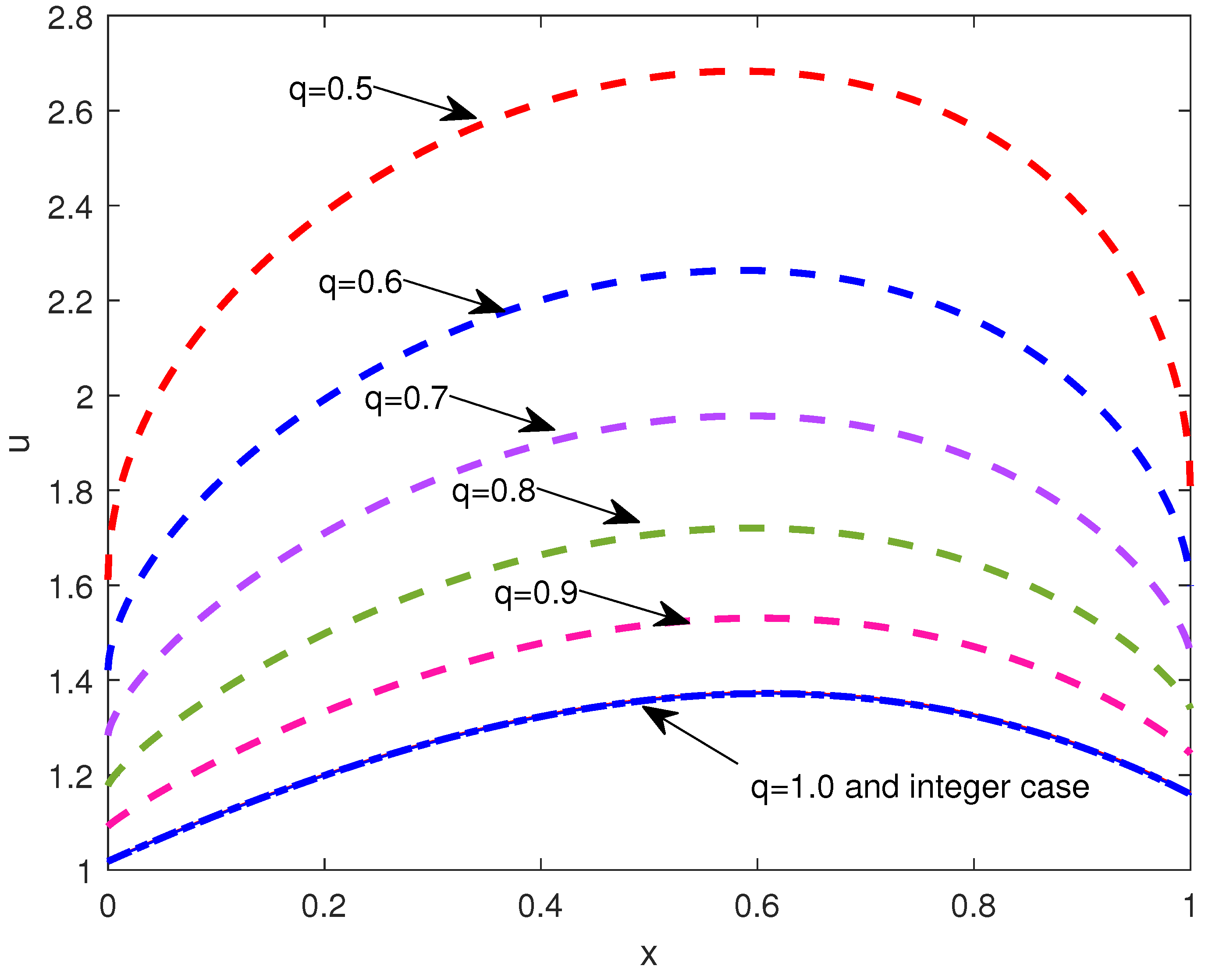
In all the four examples, we consider the terminals a and b are 0 and 1. In our first example, we consider the linear sequential Caputo fractional boundary value problem with mixed homogeneous boundary conditions:
Note that the above formula is a special case of Equation (11) with Hence:
Figure 1 represents the numerical solution of example 1, using the integral form of Equation (16) for different values of q including can be found below.
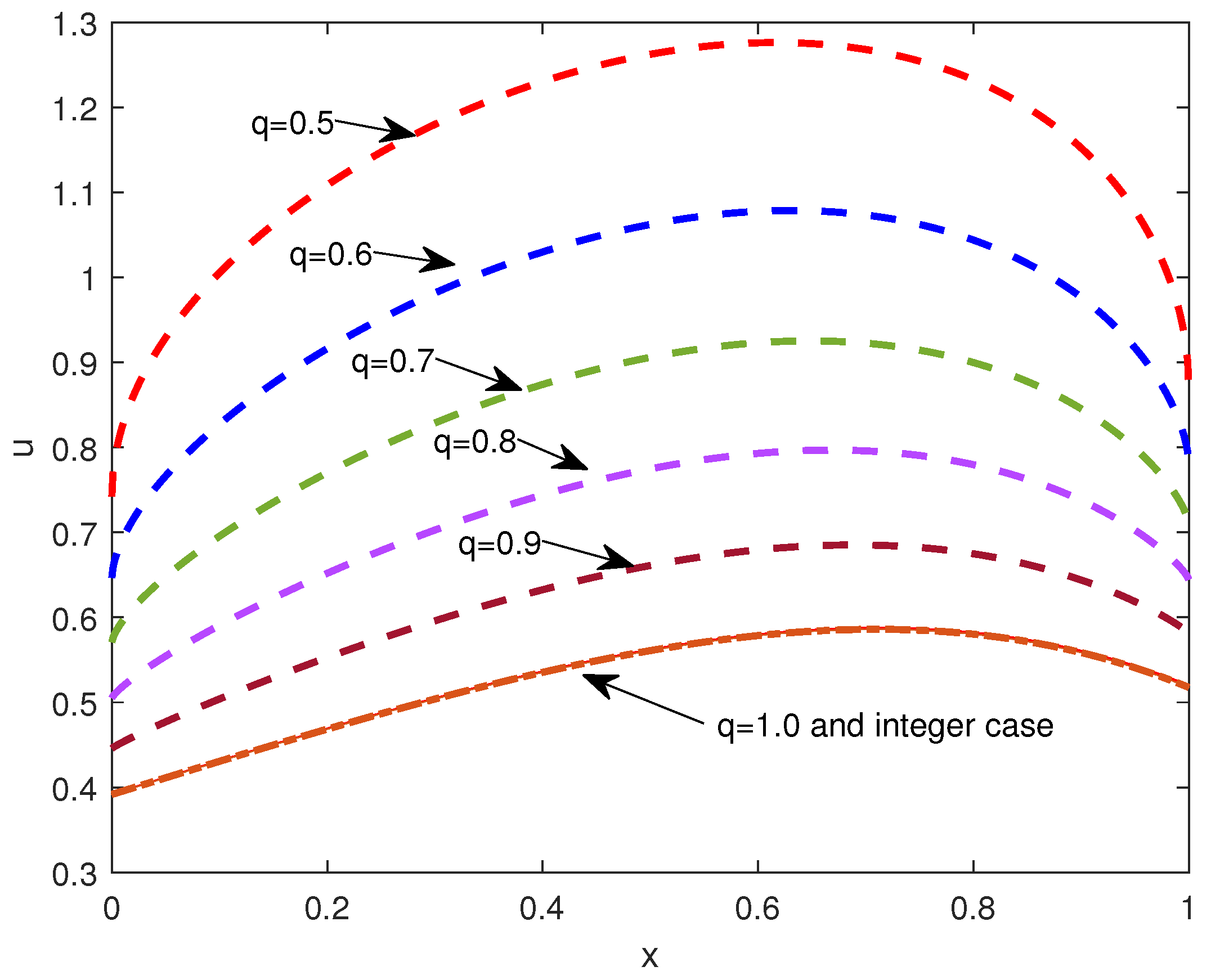
In example 2, we consider the linear sequential Caputo fractional boundary value problem with mixed boundary conditions,
The solution of Equation (19) is given by
where is the Green’s function and is the same as in example 1.
Figure 2 represents the numerical solution of example 2, using the integral form of Equation (20) for different values of q including can be found below.
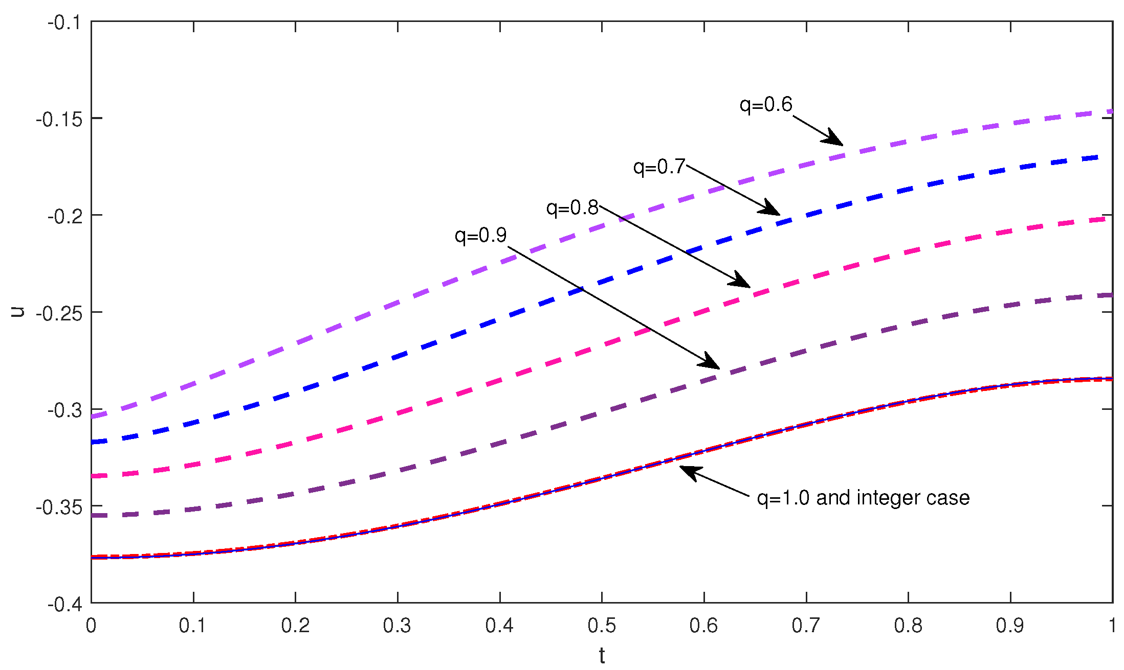
In example 3, we consider the linear sequential Caputo fractional boundary value problem with mixed boundary conditions:
The solution of Equation (21) is given by:
where is the Green’s function the same as in examples 1 and 2.
Figure 3 represents the numerical solution of example 3, using the integral form of Equation (22) for different values of q including can be found below.
In example 4, we consider the linear sequential Caputo fractional boundary value problem with mixed boundary conditions:
4. Conclusions
In this work, we have provided four numerical results for the numerical solution of linear sequential Caputo boundary value problems with Caputo type of mixed boundary conditions. In the first three examples, we considered the linear sequential boundary operator to be with mixed boundary conditions at and for three different nonhomogeneous terms. Our initial aim was to develop the numerical code for a general bounded nonhomogeneous term, so that it will be useful to solve a nonlinear problem using the generalized monotone method. However, our numerical examples helped us confirm the accuracy and validity of our code, since our numerical solution coincides with the integer solution as . It is to be noted that the Green’s function is the same in all the three examples. In our future work we will develop the code for a general nonhomogeneous term together with error analysis. We then plan to apply this to a nonlinear problem such as a (fractional) steady state population model by generalized monotone method. It is easy to observe that the Green’s function is the same for each of the linear iterates in the generalized monotone method. In addition, we can use q as a parameter to enhance the mathematical model.
In example four we considered the linear sequential Caputo boundary operator to be with the Caputo derivative of Neumann type of homogeneous boundary conditions. The Green’s function for example four is different than that of the first three examples. In this case also, our numerical solution coincides with the well known integer result. In future we plan to develop numerical code for the linear sequential Caputo boundary operator of the form with mixed Caputo boundary conditions, with general nonhomogeneous terms. This will be useful to obtain numerical solutions for the nonlinear sequential Caputo boundary value problem with mixed Caputo boundary conditions.
Author Contributions
There was equal contribution by the authors.
Conflicts of Interest
The authors declare no conflict of interest.
Appendix A
In this section we have provided the MATLAB code for all the example problems.
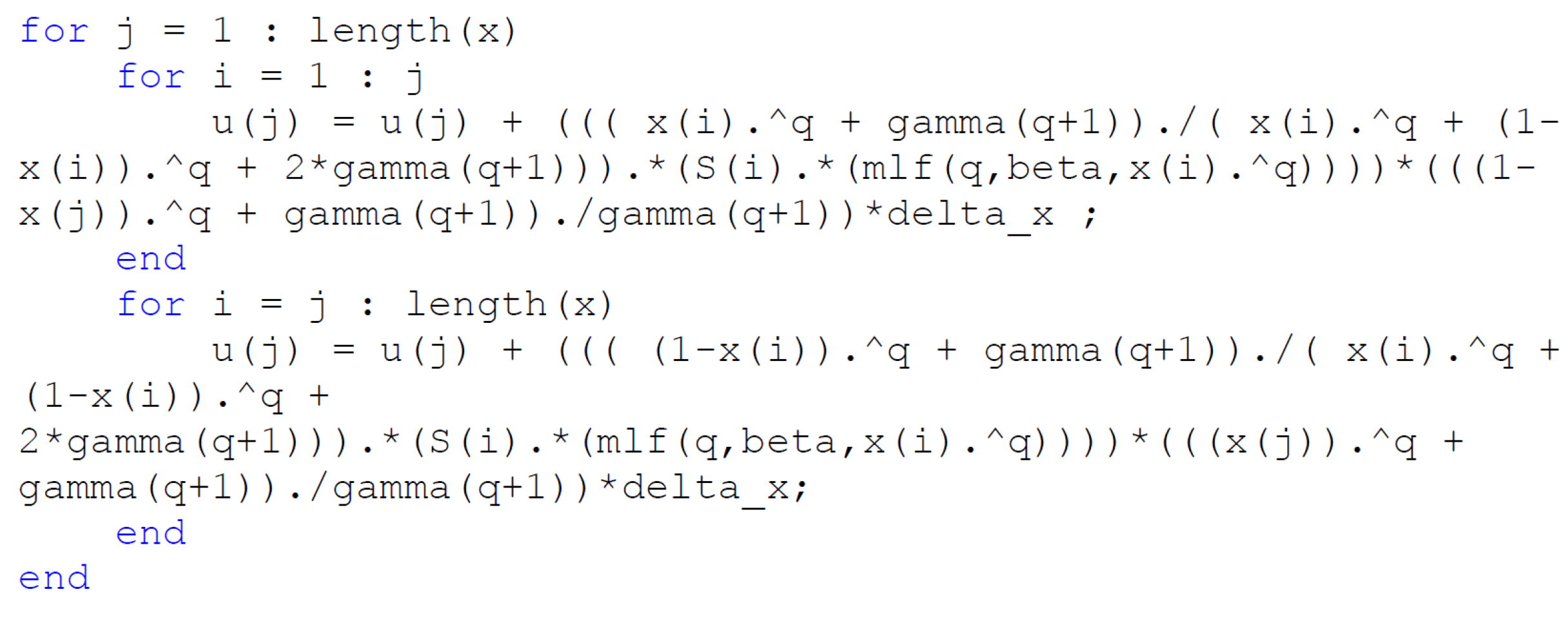
The MATLAB code for example 3 is given below. One can compute the Mittag-Leffler function using the MLF code written by Igor Podlubny. See for reference [32].
Figure A1.

The above MATLAB code is similar to examples 1 and 2 with different nonhomogeneous terms.
The MATLAB code for example 4 is given below.
Figure A2.
, where represent the cosine, sine and tangent functions.

References
- Oldham, K.B.; Spanier, J. The Fractional Calculus, Mathematics in Science and Engineering; Academic Press: New York, NY, USA, 1974. [Google Scholar]
- Ross, B. A Brief History and Exposition of the Fundamental Theory of Fractional Calculus. In Fractional Calculus and Its Applications; Lecture Notes in Mathematics; Springer: Berlin/Heidelberg, Germany, 1975; pp. 1–36. [Google Scholar]
- Tenreiro Machado, J.A.; Kiryakova, V.; Mainardi, F. A Poster About the Recent History of Fractional Calculus. Fract. Calc. Appl. Anal. 2010, 13, 329–334. [Google Scholar]
- Tenreiro Machado, J.A.; Kiryakova, V.; Mainardi, F. A Poster About the Old History of Fractional Calculus. Fract. Calc. Appl. Anal. 2010, 13, 447–454. [Google Scholar]
- Podlubny, I. Fractional Differential Equations; Academics Press: San Diego, CA, USA, 1999; Volume 198. [Google Scholar]
- Gorenflo, R.; Kilbas, A.A.; Mainardi, F.; Rogosin, S.V. Mittag-Leffler Functions, Related Topics and Applications; Springer: Berlin, Germany, 2014; p. 443. [Google Scholar]
- Kilbas, A.A.; Srivastava, H.M.; Trujillo, J.J. Theory and Applications of Fractional Differential Equations; Elsevier: Amsterdam, The Netherlands, 2006. [Google Scholar]
- Lakshmikantham, V.; Leela, S.; Devi, D.J.V. Theory of Fractional Dynamic Systems; Cambridge Scientific Publishers: Cambridge, UK, 2009. [Google Scholar]
- Ladde, G.S.; Lakshmikantham, V.; Vatsala, A.S. Monotone Iterative Techniques for Nonlinear Differential Equations; Pitman Publishing Inc.: Marshfield, MA, USA, 1985. [Google Scholar]
- Lakshmikantham, V.; Vatsala, A.S. General Uniqueness and Monotone Iterative Technique for Fractional Differential Equations. Appl. Math. Lett. 2008, 21, 828–834. [Google Scholar] [CrossRef]
- Diethelm, K.; Ford, N.J. Numerical Solution of the Bagley-Torvik Equation. BIT Numer. Math. 2002, 42, 490–507. [Google Scholar]
- West, I.H.; Vatsala, A.S. Generalized Monotone Iterative Method for Initial Value Problems. Appl. Math. Lett. 2004, 17, 1231–1237. [Google Scholar] [CrossRef]
- Kemppainen, J.; Siljander, J.; Zacher, R. Representation of solutions and large-time behavior for fully nonlocal diffusion equations. J. Differ. Equ. 2017, 263, 149–201. [Google Scholar] [CrossRef] [Green Version]
- Li, Z.; Huang, X.; Yamamoto, M. Carleman estimates for the time-fractional advection-diffusion equations and applications. Inverse Probl. 2019, 35, 045003. [Google Scholar] [Green Version]
- Tariboon, J.; Cuntavepanit, A.; Ntouyas, S.K.; Nithiarayaphaks, W. Separated Boundary Value Problems of Sequential Caputo and Hadamard Fractional Differential Equations. J. Funct. Spaces 2018, 2018, 6974046. [Google Scholar] [CrossRef]
- Ahmad, B.; Nieto, J.J.; Pimentel, J. Some boundary value problems of fractional differential equations and inclusions. Comput. Math. Appl. 2011, 62, 1238–1250. [Google Scholar] [CrossRef] [Green Version]
- Wang, G.; Ahmad, B.; Zhang, L. Some existence results for impulsive nonlinear fractional differential equations with mixed boundary conditions. Comput. Math. Appl. 2011, 62, 1389–1397. [Google Scholar] [CrossRef] [Green Version]
- Zhang, S.; Su, X. The existence of a solution for a fractional differential equation with nonlinear boundary conditions considered using upper and lower solutions in reverse order. Comput. Math. Appl. 2011, 62, 1269–1274. [Google Scholar] [CrossRef] [Green Version]
- El-Ajou, A.; Arqub, O.A.; Momani, S. Solving fractional two-point boundary value problems using continuous analytic method. Ain Shams Eng. J. 2013, 4, 539–547. [Google Scholar] [CrossRef] [Green Version]
- Anderson, D.R. Positive Green’s Functions for some fractional order boundary value problems. arXiv 2014, arXiv:1411.5616. [Google Scholar]
- Jiang, F.; Xu, X.; Cao, Z. The Positive Properties of Green’s Function for Fractional Differential Equations and Its Applications. Abstr. Appl. Anal. 2013, 2013, 531038. [Google Scholar] [CrossRef]
- Safdari, H.; Aghdam, Y.E. Numerical Solution of Green’s Function for Solving Inhomogeneous Boundary Value Problems with Trigonometric Functions by New Technique. Appl. Math. 2015, 6, 764–772. [Google Scholar] [CrossRef]
- Rehman, M.u.; Khan, R.A. A numerical method for solving boundary value problems for fractional differential equations. Appl. Math. Model. 2012, 36, 894–907. [Google Scholar] [CrossRef]
- Klimek, M. Fractional Sequential Mechanics—Models with Symmetric Fractional Derivative. Czechoslov. J. Phys. 2001, 51, 1348–1354. [Google Scholar] [CrossRef]
- Aleroev, T.S.; Kekharsaeva, E. Boundary Value Problems for Differential Equations with Fractional Derivatives. Integral Transform. Spec. Funct. 2017, 28, 900–908. [Google Scholar] [CrossRef]
- Drapaca, C.S.; Sivaloganathan, S. A Fractional Model of Continuum Mechanics. J. Elast. 2012, 107, 105–123. [Google Scholar] [CrossRef]
- Sumelka, W. Thermoelasticity in the Framework of the Fractional Continuum Mechanics. J. Therm. Stress. 2014, 37, 678–706. [Google Scholar] [CrossRef]
- Vatsala, A.S.; Sowmya, M. Laplace Transform Method for Linear Sequential Riemann-Liouville and Caputo Fractional Differential Equations. Aip Conf. Proc. 2017, 1798, 020171. [Google Scholar]
- Vatsala, A.S.; Sambandham, B. Laplace Transform Method for Sequential Caputo Fractional Dofferential Equations. Math. Eng. Sci. Aerosp. 2016, 7, 339–347. [Google Scholar]
- Sambandham, B.; Vatsala, A.S. Basic Results for Sequential Caputo Fractional Differential Equations. Mathematics 2015, 3, 76–91. [Google Scholar] [CrossRef]
- Sambandham, B.; Vatsala, A.S. Generalized Monotone Method for Sequential Caputo Fractional Boundary Value Problems. J. Adv. Appl. Math. 2016, 1, 241–259. [Google Scholar] [CrossRef]
- Podlubny, I. Mittag-Leffler Function. WEB Site of MATLAB Central File Exchange. 2006. Available online: https://www.mathworks.com/matlabcentral/fileexchange/8738-mittag-leffler-function (accessed on 03 March 2018).
Figure 1.
when .

Figure 2.
when .

Figure 3.
when .

Figure 4.
when .

© 2019 by the authors. Licensee MDPI, Basel, Switzerland. This article is an open access article distributed under the terms and conditions of the Creative Commons Attribution (CC BY) license (http://creativecommons.org/licenses/by/4.0/).
Share and Cite
MDPI and ACS Style
Sambandham, B.; Vatsala, A.S.; Chellamuthu, V.K. Numerical Results for Linear Sequential Caputo Fractional Boundary Value Problems. Mathematics 2019, 7, 910. https://doi.org/10.3390/math7100910
AMA Style
Sambandham B, Vatsala AS, Chellamuthu VK. Numerical Results for Linear Sequential Caputo Fractional Boundary Value Problems. Mathematics. 2019; 7(10):910. https://doi.org/10.3390/math7100910
Chicago/Turabian StyleSambandham, Bhuvaneswari, Aghalaya S. Vatsala, and Vinodh K. Chellamuthu. 2019. "Numerical Results for Linear Sequential Caputo Fractional Boundary Value Problems" Mathematics 7, no. 10: 910. https://doi.org/10.3390/math7100910
Note that from the first issue of 2016, this journal uses article numbers instead of page numbers. See further details here.