A Forward–Backward Simheuristic for the Stochastic Capacitated Dispersion Problem

Abstract

In an effort to balance the distribution of services across a given territory, dispersion and diversity models typically aim to maximize the minimum distance between any pair of facilities. Specifically, in the capacitated dispersion problem (CDP), each facility has an associated capacity or level of service, and the objective is to select a set of facilities so that the minimum distance between any pair of them (dispersion) is maximized, while ensuring a user-defined level of service. This problem can be formulated as a linear integer model, where the sum of the capacities of the selected facilities must match or exceed the total demand in the network. Real-life applications often necessitate considering the levels of uncertainty affecting the capacity of the nodes. Failure to account for this uncertainty could lead to low-quality or infeasible solutions in practical scenarios. However, research addressing the stochastic version of the CDP is scarce. This paper introduces two models for the CDP with stochastic capacities, incorporating soft constraints and penalty costs for violating the total capacity constraint. The first model includes a probabilistic constraint to ensure the required level of service with a certain probability, while the second model introduces a soft constraint with penalty costs for violations. To solve both variants of the model, a forward–backward simheuristic algorithm is proposed. Our approach combines a metaheuristic algorithm with Monte Carlo simulation, enabling the efficient handling of the random behavior of node capacities and obtaining reliable solutions regardless of their probability distribution.

1. Introduction

The general challenge in dispersion problems is providing a collection of elements that maximizes the diversity or representativeness of a group. In particular, the p-dispersion problem consists of selecting a subset of p elements from a given set V in such a way that the diversity between the pairs of elements (usually the pairwise distance) is maximized. This problem and other related dispersion models have been widely studied in the last few decades, and several solution approaches have been proposed to tackle them [1,2,3]. Starting with the seminal works of Kuby [4], Kuo et al. [5], and Dhir et al. [6], mostly based on integer programming models, the area of diversity and dispersion maximization has significantly grown, and constitutes an important part of location theory nowadays. A complete review of discrete diversity and dispersion maximization problems can be found in Martí et al. [7].

Consider a graph $G=(V,E)$, where V and E are the sets of elements and edges, respectively, with $\left|V\right|=n$. Let $d_{ij}>0$ be the distance between two different elements i and j, and let p be the number of selected elements. Let us define a binary variable $x_i$ that takes the value 1 if the element i is selected, and 0 otherwise. Also, we define the set of selected elements as $M=i\in V:x_i=1$. Then, the p-dispersion problem can be formulated as follows:

$$\begin{array}{ccc}\hfill \max & \hfill \underset{\begin{array}{c}i,j\in M\\ i<j\end{array}}{min}{d}_{ij}& \\ \hfill \mathrm{s}.\mathrm{t}.& \hfill {\displaystyle \sum _{i=1}^n}{x}_i=p& \\ \hfill & \hfill x_i\in \{0,1\}& i=1,2,\dots ,n\hfill \end{array}$$

(1)

The number of selected elements p is usually set in advance by the decision maker, thus ignoring practical factors that appear in many real-life situations, e.g., capacity, cost, time, etc. It is in this context that Rosenkrantz et al. [8] proposed more realistic variants of the conventional p-dispersion problem by incorporating new characteristics, e.g., the storage capacity of each facility, into the model. In particular, we focus on the capacitated dispersion problem (CDP) where the number of selected facilities is controlled by the total demand associated with the nodes in the system. As shown in Rosenkrantz et al. [8], the CDP is an NP-hard problem that belongs to the large family of facility location problems. Figure 1 depicts an example of locating similar facilities, such as shop franchises, where the goal is to avoid their proximity, since a good distribution of the facilities on the map implies reaching more people and clients. Hence, the purpose is to determine the open facilities (red stars in the example shown in Figure 1) among a set of potential candidates (marked with a location symbol) in such a way that the inter-distance between the selected facilities is maximized while, at the same time, the required demand is satisfied. Another important application of this problem is determining the location of undesirable facilities, such as landfills or sewage plants, nuclear or chemical plants, and hazardous waste sites. These facilities should be dispersed enough with the purpose of minimizing their potential social impact while satisfying storage capacity constraints [9]. An additional example involves the realistic location problem proposed in Daskin [10] and subsequently studied by Lu et al. [11], where an international branch company aims to open new offices in the U.S. to expand their business.

While uncertainty is one of the main characteristics of real-life problems, as far as we know, it has never been considered in the existing literature on the CDP. One of the main contributions of this paper is to consider a more realistic version of the CDP with stochastic capacities (SCDP). Hence, we will model the demand of each node in the network as an independent random variable. In other words, the capacity of each site is expressed as a probabilistic distribution rather than a single estimated value. The motivation for studying the stochastic variants of the CDP comes from the inherent uncertainty present in real-world situations. Traditional deterministic models, while providing foundational insights, often fall short in capturing the dynamic nature of real-life scenarios where demand and capacity can fluctuate unpredictably. By integrating stochastic elements into the model, this research aims to devise solutions that are not only near-optimal under specific conditions, but are also robust and adaptable to changes. To solve the stochastic version of the CDP, we propose a simheuristic algorithm combining Monte Carlo simulation with a metaheuristic framework [12]. Simheuristics offer a robust framework for better understanding a system’s behavior by addressing the uncertain nature of the problem. They can generate robust solutions that are less sensitive to uncertainty perturbations, ensuring that they will remain relatively insensitive to changes in the system, at least within a certain range of uncertainty. By employing a simheuristic algorithm, we can efficiently address the stochastic CDP while, at the same time, including the stochastic nature of the demands to create high-quality solutions. In particular, in our solving method, the simulation is integrated with the tabu search metaheuristic to guide the search in a way that generates robust solutions by applying perturbation operators and biased randomization techniques. Hence, the main contributions of this paper can be described as follows: (i) it proposes an extension of the deterministic CDP by considering capacities as random variables, as well as a formal description of the stochastic version, SCDP; (ii) it introduces an effective forward–backward constructive algorithm to deal with different types of instances, and a novel simheuristic algorithm to solve the SCDP; (iii) it performs a stochastic analysis of how solutions change as the level of uncertainty increases; and (iv) it provides a reliability analysis of solutions in a scenario under uncertainty.

The remainder of this paper is organized as follows. Section 2.1 and Section 2.2 contain a review of the literature on dispersion problems and stochastic location, respectively. Section 3 describes the deterministic and stochastic problems under study. Section 4.1 provides a detailed description of previous forward–backward constructive approaches to dispersion problems. Section 4.2 outlines the simheuristic tabu search method proposed to solve the SCDP. Section 5 analyzes the results obtained in our computational experiments. Finally, the conclusions of this paper are presented in Section 6.

2. Literature Review

This section provides an overview of the existing publications related to our work, including studies on diversity and dispersion problems, as well as on stochastic facility location problems.

2.1. Review of the Literature on Diversity and Dispersion Problems

As far as we know, Kuby [4] was the first author to propose diversity models in the context of discrete optimization. The author considered the p-dispersion as locating p facilities on the nodes of a network, so that the minimum distance between any pair of facilities is maximized. This problem is also known as the MaxMin dispersion problem (MMDP). The author extended this model by considering the sum of distances in the objective function, named the MaxSum diversity problem, or simply the maximum diversity problem (MDP). The survey of Martí et al. [7] reviewed the milestones in the development of diversity problems and identified three periods of time. In the early period (1980–2000), simple heuristics were applied to solve the two mathematical models, MaxSum and MaxMin, with small instances and short computational times [9,13,14,15,16]. During the expansion period (2000–2010), researchers considered other models to include different aspects of diversity, as shown in

Table 1. Diversity models.

Problem	Objective Function	Reference
MaxSum	${\displaystyle \sum _{i<j,i,j\in M}{d}_{ij}}$	Kuby [4]
MaxMin	${\displaystyle \underset{i<j,i,j\in M}{min}{d}_{ij}}$	Kuby [4]
MaxMin/Cap/Cost	${\displaystyle \underset{i<j,i,j\in M}{min}{d}_{ij}}$	Rosenkrantz et al. [8]
MaxMean	${\displaystyle \sum _{i<j,i,j\in M}{d}_{ij}/\left|M\right|}$	Prokopyev et al. [27]
MaxMinSum	${\displaystyle \underset{i\in M}{min}\sum _{j\in M,j\ne i}{d}_{ij}}$	Prokopyev et al. [27]
MinDiff	${\displaystyle \underset{i\in M}{max}\sum _{j\in M,j\ne i}{d}_{ij}-\underset{i\in M}{min}\sum _{j\in M,j\ne i}{d}_{ij}}$	Prokopyev et al. [27]

. They introduced larger instances that pose a challenge to simple heuristics and applied complex metaheuristics to efficiently solve the problems [17,18,19,20,21,22]. Finally, in the development period (2010–2023), researchers mainly worked on sophisticated metaheuristics to obtain high-quality solutions to instances of very large problems [23,24,25,26].

Our work analyzes an extension of the model introduced by Rosenkrantz et al. [8]. Specifically, these authors considered the inclusion of capacity constraints motivated by their practical applications in facility location. The resulting CDP model was built upon the classical MaxMin objective function by replacing the typical cardinality constraint of p elements with a constraint with the required capacity (specifying the desired level of service). Several papers on the CDP have been identified. The first one was by Peiró et al. [28], who adapted a GRASP method which had already been implemented for the unconstrained MaxMin diversity to this constrained variant [3,7,29]. The  GRASP method of solving the CDP implements a strategic oscillation [30] for an efficient search of the solution space. This proposal was able to outperform the previous heuristic method by Rosenkrantz et al. [8]. In a different work, Martí et al. [31], proposed a mathematical model and a heuristic based on the scatter search (SS) methodology to improve the previous results for the CDP. The authors adapted the exact method by Sayyady and Fathi [32] for the MaxMin to the CDP. The method iteratively solves the node packing problem, which finds a maximum cardinality subset of nodes in an auxiliary graph, so that no two nodes in this subset are adjacent to each other. With this method they were able to solve medium size instances to optimality. The SS method explores the solution space by improving and combining a small set of solutions. The combination method applies path relinking [33], which generates new solutions by connecting high-quality solutions. It implements a local search that, starting from one of these solutions, swaps its elements one by one with the elements in another high-quality solution. In yet another work, Mladenović et al. [34] customized the variable neighborhood search (VNS) methodology to further improve upon their previous results for the CDP. This method is able to reach all of the best-known solutions to the CDP established in the literature. Gomez et al. [35] proposed a multi-start biased randomized algorithm to efficiently solve the instances in the testbed. Furthermore, Lu et al. [11] introduced a solution-based tabu search algorithm, which incorporated a hash-based mechanism to rapidly identify eligible neighboring solutions and employed a streamline calculation strategy to quickly determine the objective function value of a neighboring solution. The aforementioned studies have significantly contributed to the analysis of the CDP, and are able to solve medium-sized and large-sized instances. However, one major limitation can be identified in these previous works: they targeted the CDP in its deterministic version, without considering the stochastic nature of real-life scenarios.

2.2. Related Work on Stochastic Facility Location Problems

Since there are no previous articles on the stochastic versions of the CDP, a review of the existing work on the more general stochastic facility location problem (FLP) is provided. Some of the seminal articles which incorporated uncertainty into FLP models made use of the mean-variance objective function. For instance, Jucker and Carlson [36] considered a stochastic version of the FLP with random demands. Following these ideas, Hodder and Jucker [37] also took into account the existence of possible correlations among random demands in their model. Another early work is that of Drezner [38], who considered an FLP with uncertainties caused by disruptions. With the aim of minimizing customers’ total traveling and waiting costs, Wang et al. [39] analyzed an FLP with stochastic demands. The authors developed several heuristic approaches, including a greedy-dropping procedure, a tabu search (TS) algorithm, and an optimal-epsilon branch-and-bound method. After a series of experiments, they concluded that the greedy heuristic is the fastest method, but it might provide sub-optimal solutions in many cases. On the contrary, the optimal-epsilon method and the TS algorithm provided high-quality results, even though the former required much larger computational times than the latter. Ravi and Sinha [40] proposed a two-stage stochastic optimization model for solving the FLP, where the demand of each customer is not known during the first stage. Hence, each facility has a first-stage opening cost and a recourse cost in case it was not opened in the first stage.

A review of the stochastic FLP is provided in Snyder [41]. This review illustrates different optimization approaches that have been applied to solve stochastic versions of the problem. Baron et al. [42] analyzed a version of the FLP in the presence of stochastic demand and congestion. Indicators such as the level of service and the maximum travel distance were also considered. Wagner et al. [43] considered an FLP variant in which the demands are stochastic and correlated. These authors proposed a mean-variance approach that balanced profit and uncertainty. Verma et al. [44] made use of fuzzy logic to model the FLP under uncertainty and solve some small-sized instances. Contreras et al. [45] considered a stochastic FLP variant in which random traffic flows from one node have to be routed to their final destination via different hub facilities. In Arabani and Farahani [46], the authors discuss several characteristics associated with FLPs, and they dedicated a section to its probabilistic, fuzzy, and stochastic versions. Likewise, Correia and da Gama [47] proposed different modeling frameworks for the FLP under uncertainty and discuss the differences between robust optimization, stochastic programming, and chance-constrained models. Similarly, Lu et al. [48] proposed a model with random disruptions. These authors applied a robust optimization approach to minimize the expected cost under a worst-case scenario. Kim et al. [49] considered a stochastic FLP based on drone facilities applied to humanitarian logistics, which forced them to consider uncertainty in the drone operating conditions. Since the application requires short computational times, the authors developed a heuristic algorithm based on the Benders decomposition. Still, one clear limitation of their approach is the assumption that the flight distance of a drone follows an exponential probability distribution. Abensur et al. [50] proposed the combined use of game theory and simulations to analyze an FLP under an uncertainty scenario. Another singular aspect of this work is the application context, which is not the traditional logistics one, but one related to financial services.

Parragh et al. [51] considered a bi-objective stochastic FLP, in which cost and covered demand have to be optimized, being the latter being a random variable with a known probability distribution. These authors applied the L-shaped method for stochastic programming, which is combined with a branch-and-bound method. Since these methods are expensive in terms of computational time, the authors recommended some techniques that might speed up computations, which is specially useful in the case of real-life applications. With the goal of minimizing unsatisfied demand and response time, Turkeš et al. [52] proposed a matheuristic algorithm for the stochastic facility location problem with different facility sizes and stored goods. The authors assumed different sources of uncertainty, including demands, inventory spoilage, and availability of the transportation network. Their matheuristic combines an iterated local search, which searches for promising location and inventory configurations, with the use of an exact solver, which optimizes the assignment problem associated with each given configuration. Finally, Ref. [53] analyze reliability aspects of an FLP with uncertain disruptions. These authors made use of a robust optimization approach, which employs a cutting plane algorithm. A simulation was then used to verify the performance of their models.

3. Problem Description and Formulation

Our stochastic models will build upon the mathematical programming model proposed by Rosenkrantz et al. [8] for the deterministic version of the CDP. In this section we first describe a mathematical model for the deterministic CDP (Equation (2)). Subsequently, we introduce two stochastic versions of the CDP: the stochastic CDP with a probabilistic constraint (SCDP-PC, Equation (3)), and the stochastic model with a soft constraint (SCDP-SC, Equation (4)).

Consider a set of locations (nodes) V, with $\mid V\mid =n$, such that $d_{ij}>0$ represents the distance between two different sites i and j, with $d_{ij}=d_{ji}$. Let $c_i\ge 0$ be the storage capacity of a site $i\in V$. Let us consider a binary variable $x_i$ that takes the value 1 if site i is selected, and 0 otherwise. Let $B>0$ be the aggregated demand requested by the nodes in the network. Then, the deterministic CDP consists of finding a subset $M\mathrm{s}\mathrm{u}\mathrm{b}\mathrm{s}\mathrm{e}\mathrm{t} V$ with a total storage capacity which is larger than the aggregated demand B, in such a way that the dispersion of the selected sites is maximized. If we denote that $M=\{i\in V:x_i=1\}$, the formulation of the (deterministic) CDP is as follows:

$$\begin{array}{cccc}\hfill & \hfill & \hfill max& \underset{\begin{array}{c}i,j\in M\\ i<j\end{array}}{min}{d}_{ij}{x}_i{x}_j\hfill \\ \hfill & \hfill & \hfill \mathrm{s}.\mathrm{t}.& {\displaystyle \sum _{i=1}^n}{c}_i{x}_i\ge B\hfill \\ \hfill & \hfill & \hfill & x_i\in \{0,1\}\hfill & \hfill & \forall i\in V\hfill \end{array}$$

(2)

The objective function and the definition of the variables are the same as in the p-dispersion problem. However, the sites are selected in such a way that their total storage capacity is at least capacity level B.

Two stochastic versions of the CDP are introduced next. The first one has random capacities and a probabilistic constraint (SCDP-PC). We assume that the storage capacity $c_i$ of each site $i\in V$ is not known in advance. However, it can be modeled using a probability distribution whose specific values will be revealed once the sites have been already selected. Then, each site has an associated independent random variable ${\tilde{C}}_i>0$ ($\forall i\in V$) which follows a non-negative probability distribution, such as the Weibull or the log-normal ones. In many stochastic problems, a recourse action can be applied when the solution is not feasible in a given scenario, usually called a ‘solution failure’. However, in our problem we do not always have this possibility. A solution specifies a set of locations, in which some facilities will be temporarily located (e.g., communication antennas) or permanently built (e.g., hospitals, clinics, coffee shops, etc.). In the second case, if they cannot reach the requested demand in a given scenario, there is no easy way to consider a recourse action. For that reason, it is necessary to compute the reliability associated with a proposed solution in a scenario under uncertainty, i.e., the probability that the solution performs as intended without failure. Hence, a probabilistic constraint model can be formulated as follows:

$$\begin{array}{cccc}\hfill & \hfill & \hfill max& \underset{\begin{array}{c}i,j\in M\\ i<j\end{array}}{min}{d}_{ij}{x}_i{x}_j\hfill \\ \hfill & \hfill & \hfill \mathrm{s}.\mathrm{t}.& P\left(\sum _{i\in V}{\tilde{C}}_i{x}_i\ge B\right)\ge \alpha \hfill \\ \hfill & \hfill & & x_i\in \{0,1\}\hfill & \hfill & \forall i\in V\hfill \end{array}$$

(3)

In the second stochastic model, we consider random capacities and soft constraints (SCDP-SC). As before, V is the set of all sites with independent random capacity variables ${\tilde{C}}_i>0$ and B is the required aggregated demand. The distances between each pair of sites, $(i,j)\in V$, are also constant values. Instead of assuming a probabilistic constraint, we consider a soft constraint with a recourse strategy, which includes a ‘penalty cost’ in the objective function. If the soft constraint is satisfied, i.e., if the aggregated demand is covered by the capacity of the facilities in the current solution, then the solution U is simply defined as the set M of selected facilities, i.e., $U=M=\{i\in V:x_i=1\}$. However, if the soft constraint is not satisfied and the aggregated demand exceeds the current capacity, then we consider the solution U as the set M with the selected facilities, together with the set R of additional facilities (selected at random) to meet the original demand B plus an additional demand that is imposed as a penalty cost. Then, the mathematical model can be stated as follows:

$$\begin{array}{cccc}\hfill & \hfill & \hfill max& \underset{\begin{array}{c}i,j\in U\\ i<j\end{array}}{min}{d}_{ij}\hfill \\ \hfill & \hfill & & x_i\in \{0,1\}\hfill & \hfill \forall i\in V\end{array}$$

(4)

where:

$$U=\left\{\begin{array}{cc}M\hfill & \mathrm{if}\sum _{i\in V}{\tilde{C}}_i{x}_i\ge B\hfill \\ \\ M\cup R\hfill & \mathrm{otherwise}\hfill \end{array}\right.$$

(5)

In other words, when M is infeasible we compute $U=M\cup R$ by adding randomly selected facilities to R until an extra level of service is met. In our computational experiments, this new demand to achieve during the recourse process exceeds the original one by a given percentage, representing the penalty cost for initially violating the soft constraint.

4. Solution Methods

Many metaheuristics, including those based on artificial intelligence, social behavior, or bio-inspired techniques, have been proven to be effective in solving complex optimization problems [30,54,55,56,57]. In Martí et al. [7], tabu search (TS) is identified as the most successful metaheuristic for solving diversity maximization problems. This makes TS a natural choice for addressing the stochastic CDP. In this section, we first review the state-of-the-art methods published using constructive–destructive metaheuristics to solve related dispersion problems, and then we propose a new one. Specifically, we describe a TS to solve the deterministic model, which is then extended into a simheuristic to address the stochastic versions of the CDP.

4.1. Previous Constructive-Destructive Neighborhood Searches

There are several research papers that propose using constructive–destructive neighborhood searches to design approaches for solving problems. For instance, Aringhieri et al. [58] explore both constructive and destructive approaches for solving the MaxSum and MaxMinSum diversity problems. Glover et al. [59] proposed two constructive and two destructive heuristics. The first constructive (C1) and destructive (D1) methods were based on the concept of the center of gravity of a set, computed as the average of the elements’ coordinates. Algorithm C1 selects, at each step, the element with the maximum distance to the center among the elements already selected. The method finishes when p elements have been selected. Conversely, starting with all elements selected, D1 removes, at each step, the element with the minimum distance to the center from among the selected elements. The method finishes when $n-p$ elements have been removed, leaving only p elements selected. The other two heuristics in Glover et al. [59], namely C2 and D2, have been extensively applied in metaheuristic methods for discrete diversity optimization. C2 selects, at each step, the element with the maximum distance to the already selected elements, while D2 removes, at each step, the element with the minimum distance to the set of selected elements until only p elements remain selected. Here, the distance of an element from a set is computed either as the sum of distances to the elements in the set or the minimum of those distances, depending on whether we are solving the MaxSum or MaxMin problem, respectively. Building upon each of the four methods described above, Duarte and Martí [21] proposed a greedy randomized adaptive search procedure (GRASP) metaheuristic to address the limitations of these greedy methods. The idea of complementing constructive methods with destructive ones has been applied in various diversity problems. See, for example, the works of Peiró et al. [28] and Lozano and Rodríguez [54]. Peiró et al. [28] applied a strategic oscillation framework, alternating between the constructive and destructive methods proposed in Glover et al. [59] (C1 and D1) to solve a capacitated version of the maximum diversity problem. The C1 constructive method incrementally adds elements to the partial solution under construction until the capacity level is satisfied, resulting in a feasible solution, say $M_1$. Subsequently, the authors proposed to “keep going” by adding some extra elements to $M_1$ using C1, obtaining solution $M_2$. Then, D1 was applied to remove some elements from $M_2$, potentially yielding a new feasible solution, $M_3$, which may be superior to the previous ones. This iterative process continues, with D1 removing some extra elements from $M_3$, resulting in a partial, infeasible solution $M_4$ that does not meet the capacity constraint.

4.2. A Hybrid Simheuristic Algorithm

Probabilistic modeling emerges as one of the most effective techniques for capturing uncertainty in real-life optimization problems [60,61]. In particular, simheuristics hybridize simulation techniques with metaheuristics to address stochastic optimization problems [12]. Simheuristics have demonstrated successful applications in solving combinatorial optimization problems across various domains, such as production [62]. They are built up from an efficient heuristic in which a stochastic evaluation is repeatedly computed at strategic points of the algorithm. This allows us to obtain a more ‘robust’ final solution, i.e., one that performs well under a stochastic scenario. We first describe our base metaheuristic, a probabilistic TS, to solve the deterministic CDP. Then, this metaheuristic is extended into a simheuristic to solve the stochastic version of the stochastic CDP.

4.2.1. A Probabilistic Tabu Search Algorithm

To solve the deterministic CDP, our approach has two phases. In the first one, a tailored method generates a solution based on the type of instance being solved. To do it, we propose two construction methods, BR-F and BR-B heuristics, and apply them for a few trials first to select the best one with a reactive mechanism. Then, the selected method is repeatedly applied, following a classic multi-start pattern. The constructed solutions are then submitted to a TS improvement method. We then make use of biased-randomization (BR) techniques to add/remove nodes from an emerging solution. These techniques make use of skewed probability distributions to transform a deterministic heuristic into a probabilistic algorithm able to generate many ‘good-quality’ solutions to the problem in short computational times [63]. The term ‘forward heuristic’ refers to the constructive method, while the term ‘backward heuristic’ refers to the destructive one. The bias randomized forward heuristic (BR-F) starts with an empty initial solution S. The algorithm adds nodes from V to the solution S, while the capacity constraint is not satisfied (Algorithm 1). As input parameters, the method requires the instance I to be solved, the parameter $\delta$ to balance the distance, and the capacity of the greedy function (6). I contains the information about the capacity of each element i, $c_i$, the minimum required level of capacity B, and the distance between any pair of elements $d_{ij}$, $e=(i,j)\in E$. S is initialized as an empty solution in step 1. Let $edge{s}_{l}ist$ be the list with all the edges in the input graph. In step 2, the algorithm sorts this list of edges in a decreasing order based on the distances between nodes, where the largest edge comes first (we call the ordered list $edge{s}_{l}is{t}_{\downarrow }$). We then randomly select one of the edges according to a geometric probability distribution. This biased selection favors the edges with larger distances (i.e., in the first positions in the list). Specifically, in step 3, the edge $e=(i_0,j_0)$ is randomly selected from the $edg{e}_{l}is{t}_{\downarrow }$. The endpoints of edges e, $i_0$, and $j_0$, are added to the partial solution, and their objective functions are initialized in step 5 with the distance between $i_0$ and $j_0$ being $d_e=d_{i_0{j}_0}$. The objective function value $f\left(S\right)$ of the partial solution S is then updated (step 5). The BR-F performs iterations, adding an element at a time, to reach the required level of service. The while loop in Algorithm 1 shows these iterations (from steps 7–13). In particular, the method first creates a candidate list, $CL$, with all the elements not included in the solution (i.e., $CL=V\setminus S$). The candidate elements in $CL$ are evaluated considering both their distance to the elements already in the solution S, and their capacity. In mathematical terms, for each node $i\in CL$ we compute its evaluation $g\left(i\right)$ as:

$$g\left(i\right)=\delta ·d(S,i)+(1-\delta )·c\left(i\right)$$

(6)

where $d(S,i)$ is the minimum distance from node i to the elements in S, and $c\left(i\right)$ is the capacity of elements i, or $c_i$. Both distance and capacity are normalized in order to sum them up. To set up the $\delta$ parameter, the constructive heuristic is executed 10 times, varying the range of $\delta$ from 0 to 1 and increasing its value by $0.1$ in each execution. Subsequently, the $\delta$ value associated with the best solution found is utilized throughout the entire execution. This parameter in the greedy function oversees the balance between distance and capacity. Once all the elements are computed, they are rearranged by applying a biased-randomized process, so the elements associated with higher values are more likely to be ranked at the top of the list. This process allows us to select the elements in a different order at each iteration of the process, while still preserving the flavor of the original heuristic. In our case, a geometric probability distribution, driven by a single parameter $\beta$ ($0<\beta <1$), is used to induce this skewed behaviour. The value of this parameter was set after a quick tuning process over sample of deterministic CPD benchmark instances. Thus, this selection returns the element $i^{*}$ of $CL$ to be added to the solution (step 9). After adding it to the solution (step 10), the objective function is updated (step 11), and the element is removed from the candidate list (step 12). The algorithm finishes when the capacity level B is satisfied.

Algorithm 1 BR-F(I, $\delta$)

1: $S\leftarrow \varnothing$   2: $edges\_lis{t}_{\downarrow }\leftarrow \mathit{sort}\_\mathit{decrease}(edges\_list)$   3: $(i_0,j_0)\leftarrow \mathit{random}\_\mathit{select}\_\mathit{edge}(edges\_lis{t}_{\downarrow })$   4: $S\leftarrow S\cup \left\{i_0\right\}\cup \left\{j_0\right\}$   5: $f\left(S\right)\leftarrow d_{i_0{j}_0}$   6: $CL\leftarrow V\setminus S$   7: while  $\mathit{not}\_\mathit{feasible}\left(\mathit{S}\right)$  do   8:     $CL\leftarrow \mathit{sort}\_\mathit{descending}(CL,g)$   9:     $i^{*}\leftarrow Geom\_selects\_node\left(CL\right)$ 10:     $S\leftarrow S\cup \left\{i^{*}\right\}$ 11:     $f\left(S\right)\leftarrow Update\_f\left(S\right)$ 12:     $CL\leftarrow CL\setminus \left\{i^{*}\right\}$ 13: end while 14: return  S

In terms of computational complexity, the bias randomized forward heuristic exhibits a Big O notation of $O\left(n^2\right)$. This complexity arises from the necessity to sort the edge list in increasing distance order and the iterative process of selecting and removing nodes based on the geometric probability distribution until the capacity constraint is satisfied. It must be noticed that, since we are solving the stochastic version of the capacity diversity problem, the elements (also called sites) have random capacity variables $\tilde{C}i>0$, and at this stage of the solving method (i.e., when constructing solutions), we are considering their expected value as the input in the algorithm.

The bias randomized backward heuristic (BR-B) follows the line drawn by destructive heuristics such as GRASP-D1 [21]. Similarly to BR-F, the BR-B algorithm requires the instance information I as its input (Algorithm 2). In contrast to BR-F, BR-B starts with all elements selected (step 1), and removes nodes from the solution S as long as it continues to fulfill the capacity constraint (while loop, from steps 3–7). The algorithm creates an edge list sorted in increasing distance order, which we call $edge{s}_{l}is{t}_{\uparrow }$ (step 2). While the solution remains feasible, the algorithm selects an edge $e^{*}$ at random using a geometric probability distribution based on the distances of the edges. Then, the next element to be removed from the solution (step 6) is selected at random from the two nodes of the edge $e^{*}$. The probability of selecting a node $i^{*}$ of $e^{*}$ is inversely proportional to its capacity, i.e., the lower its capacity, the larger the probability (step 5). To ensure the feasibility of the solution, the last removed element is reinserted after the while loop (step 8).

Algorithm 2 BR-B(I)

1: $S\leftarrow V$ 2: $edges\_lis{t}_{\uparrow }\leftarrow \mathit{sort}\_\mathit{increase}(edges\_list)$ 3: while  $\mathit{feasible}\left(\mathit{S}\right)$  do 4:     $e^{*}\leftarrow Geom\_selects\_edge(edges\_lis{t}_{\uparrow })$ 5:     $i^{*}\leftarrow random\_select\_node\left(e^{*}\right)$ 6:     $S\leftarrow S\setminus \left\{i^{*}\right\}$ 7: end while 8: $S\leftarrow S\cup \left\{i^{*}\right\}$ 9: return  S

Similar to the BR-F heuristic, the bias randomized backward heuristic also plays a central role in our solution methodology, offering a destructive counterpart to the constructive nature of BR-F. The computational complexity is $O\left(n^2\right)$, attributable to the algorithm’s need to evaluate each node and edge in the process. Both algorithms operate with a loop that continues until a feasible solution is found. This setup implies that, when fewer nodes are needed, the constructive strategy arrives at a solution quicker than its destructive counterpart. In some real-life applications, such as logistics or transportation, a solution with a small fraction of the number of facilities opened usually satisfies the total demand. However, in other applications, such as telecommunications or smart cities with the IoT, the required number of open facilities is usually very large to meet the capacity requirements. This is why we propose two different constructive methods considering the different types of instances to be solved. Notice that, in the first type of applications, a construction method would perform a low number of iterations, but in instances of the second type of applications, it would perform a large number of iterations, and it seems more appropriate to apply a destructive method there. Our BR-F and BR-B heuristics complement each other and together offer a robust solution for any situation.

Algorithm 3 illustrates the pseudocode of our TS for the CDP. The algorithm receives the constructed solution S and the maximum number of iterations without improvement, $i{t}_{max}$, as inputs. Let $S^{\prime }$ be the best solution, which initially is $S^{\prime }=S$ (step 1). From step 3 to 13, the method sequentially drops the oldest selected element u in S (steps 5 and 6), and adds the element $u^{*}$ with the maximum–minimum distance from $u^{*}$ to $S\setminus u$ (step 7). Ties with respect to the max–min value are broken with the element which maximizes the sum of the distances to the elements in $S\setminus u$ (step 8). If the new solution $S=(S\setminus u)\cup u^{*}$ improves the best solution identified so far, $S^{\prime }$, then it is updated (steps 9 to 12). The algorithm ends after $i{t}_{max}$ iterations without improvement and returns the best solution it found (step 14).

The TS improvement operates with an $O(nlogn)$ complexity per iteration, accounting for the management of the tabu list and neighborhood explorations. Consequently, the overall complexity of the probabilisitic tabu search (PTS) algorithm can be succinctly described as $O(n^2+i{t}_{\max }·nlogn)$, achieving a balance between the initial solution formulation and an efficient TS, where $i{t}_{\max }$ represents the iterations without improvement. As mentioned, the construction can be either the BR-F method, described in Algorithm 1, or the BR-B method, described in Algorithm 2. The method requires three input parameters: the instance I, the parameter $\delta$ obtained from the construction phase, and $i{t}_{\max }$ from the TS algorithm.

4.2.2. Extending the PTS to a Simheuristic Approach

In this section, we extend the PTS using the simheuristic framework [12], introducing simulation techniques to evaluate the performance of promising solutions in a stochastic environment. As documented in the stochastic literature, good deterministic solutions improve the chances of finding better stochastic solutions. In this vein, we adapt the PTS algorithm to the simheuristic framework, considering its ability to achieve very good outcomes (see Section 5).

Algorithm 3 Probabilistic Tabu Search, PTS($S,i{t}_{max}$)

1: $S^{\prime }\leftarrow S$   2: $\mathit{noImprovement}\leftarrow 0$   3: while  $\mathit{noImprovement}<{\mathit{it}}_{\mathit{max}}$  do   4:      $\mathit{noImprovement}\leftarrow \mathit{noImprovement}++$   5:      $u\leftarrow \mathit{select}\_\mathit{oldest}\_\mathit{node}\left(S\right)$   6:      $S\leftarrow \mathit{Drop}(S,u)$   7:      $u^{*}\leftarrow \mathit{select}\_\mathit{best}\_\mathit{node}(V\setminus S)$   8:      $S\leftarrow \mathit{Add}(S,u^{*})$   9:     if $f\left(S\right)>f\left(S^{\prime }\right)$ then 10:         $S^{\prime }\leftarrow S$ 11:          $\mathit{noImprovement}\leftarrow 0$ 12:     end if 13: end while 14: return  $S^{\prime }$

In Section 3, we described two stochastic variants for the CDP: the stochastic model with a soft constraint (SCDP-SC), and the stochastic model with random capacities and a probabilistic constraint (SCDP-PC). The first model, with soft constraints (Equation (4)), penalizes the objective function value by selecting more than the required elements (e.g., a $25\%$ of extra facilities are randomly opened) in scenarios where the soft constraint is not satisfied. In such cases, the penalized objective function value is computed as the minimum distance between all pairs of selected sites. Note that this value is significantly worse (lower) than the original objective function value of the solution. The recourse action of selecting extra elements is a raw strategy but is very effective, as it ensures that a robust solution can be found for different stochastic scenarios. Algorithm 4 illustrates the main steps of our simheuristic approach for the SCDP-SC, which we call SimTS-SC.

Algorithm 4 takes the maximum number of iterations $i{t}_{max}$ without improvement and the maximum time $t_{max}$ as inputs, and consists of three main phases.

Table 2. Symbols and Definitions.

Symbol	Definition
S	solution
$S^{*}$	best solution
$s\mathcal{P}$	set of stochastic solutions
$sf\left(S\right)$	stochastic objective function value of solution S, i.e., average of the objective function value in different scenarios
$\nu \left(S\right)$	estimation of the reliability level, i.e., the estimated probability that the solution S is still feasible once a scenario takes place

summarizes the parameters and symbols used in this method. In the initial phase, the algorithm generates a feasible solution that is improved with the TS algorithm (step 1). This initial solution $S^{*}$ is the best solution known so far. Then, a fast simulation is performed to obtain the average value of the objective function (minimum distance) of the simulations performed over that solution, denoted as $sf\left(S^{*}\right)$, i.e., the stochastic objective function evaluation (step 2). The pool of best stochastic solutions $s\mathcal{P}$ is initialized with the best solution $S^{*}$ (step 3). In the second phase, a while loop is executed to generate new solutions (step 5). They are obtained by applying the PTS algorithm to the instance with expected values. Then, only a short number of simulations runs are conducted on the promising solutions (steps 6 and 7) to evaluate the quality of each of these solutions in a stochastic environment. In each iteration, if the new promising solution shows a higher stochastic objective function value than the current best solution, it is updated and inserted into the set of best stochastic solutions $s\mathcal{P}$ (step 10). Finally, in the third phase, an extended simulation experiment is conducted on the best stochastic solutions found (steps 14–19), which provides a more accurate estimate of the expected objective function value. Furthermore, this intensive simulation also provides relevant statistics to analyze the reliability of each solution in $s\mathcal{P}$, and the best one is returned by the algorithm (step 20).

Algorithm 4 SimTS-SC(I, $\delta$, $t_{max}$, $i{t}_{max}$)

1: $S^{*}\leftarrow \mathtt{PTS}(I,\delta ,i{t}_{max})$   2: $(S^{*},sf\left(S^{*}\right))\leftarrow \mathit{Simulation}(S^{*},\mathit{short})$   3: $s\mathcal{P}\leftarrow add\left(S^{*}\right)$   4: while  $time\le t_{max}$  do   5:     $S\leftarrow \mathtt{PTS}(I,\delta ,i{t}_{max})$   6:     if $f\left(S\right)>f\left(S^{*}\right)$ then   7:         $(S,sf(S\left)\right)\leftarrow \mathit{Simulation}(S,\mathit{short})$   8:         if $sf\left(S\right)>sf\left(S^{*}\right)$ then   9:            $S^{*}\leftarrow S$ 10:            $s\mathcal{P}\leftarrow \mathit{add}\left(S^{*}\right)$ 11:         end if 12:     end if 13: end while 14: for  $S\in s\mathcal{P}$  do 15:     $(S,sf(S\left)\right)\leftarrow \mathit{Simulation}(S,\mathit{long})$ 16:     if $sf\left(S\right)>sf\left(S^{*}\right)$ then 17:         $S^{*}\leftarrow S$ 18:     end if 19: end for 20: return  $S^{*}$

The SimTS-SC algorithm, incorporating the PTS, exhibits a computational complexity of $O(n^2+i{t}_{max}·nlogn)$. The inclusion of short-term simulations adds a complexity of $O(shortsim·n)$ due to the evaluation of each node being included in the solution, resulting in an overall complexity of $O(n^2+i{t}_{max}·nlogn+shortsim·n)$. In the second stochastic model SCDP-PC—see Equation (3)—the objective function remains unchanged with variations in the expected capacity values across different scenarios. However, the stochastic nature of the model arises from the probabilistic constraint, which assesses the probability of the solution satisfying the capacity constraint. The simheuristic algorithm for the SCDP-PC, denoted as SimTS-PC, follows the main steps outlined in Algorithm 4. However, it differs in two aspects related to construction and evaluation, which are adapted to accommodate the stochastic nature of the problem. When constructing a solution using the PTS algorithm, the iterative process of adding elements to the solution (opening facilities) terminates when the probabilistic constraint is satisfied. Additionally, instead of evaluating the objective function $sf\left(S\right)$, which remains constant in this model, the simulation process provides an estimation of the reliability level, denoted as $\nu \left(S\right)$, associated with the current solution S (steps 2, 7, and 15 in Algorithm 4). As explained before, the reliability level of a solution S represents the probability that the solution S is feasible when a scenario occurs. Figure 2 presents a multi-dimensional comparison between two methodologies: PTS and SimTS. The chart assesses each methodology across six distinct performance metrics: optimality, speed, flexibility, uncertainty, scalability, and reliability. Each axis corresponds to one of these metrics, extending outward from the center where the lowest value is located, and higher values are depicted further from the center. The performance of SimTS is depicted by the green line, whereas the performance of PTS is illustrated by the black line.

SimTS demonstrates a superior performance in handling uncertainty and ensuring reliability, thanks to the simulations integrated into the algorithm. These simulations also result in significant computational times. Consequently, there is a relative decrease in speed and optimality under the deterministic conditions compared to the PTS algorithm. Therefore, in terms of scalability, SimTS may face challenges with larger instances where PTS excels. Nonetheless, SimTS exhibits greater flexibility, allowing it to effectively manage more dynamic and variable environments.

5. Computational Experiments

In this section, we first evaluate the performance of our simheuristic algorithm SimTS-PC when solving the stochastic model with a probability constraint (SCDP-PC). Then, we assess the performance of our simheuristic algorithm SimTS-SC when solving the stochastic model with soft constraints (SCDP-SC). For each of these experiments, we performed the following steps: (i) compare the solving method for the deterministic model (PTS) with our simheuristic algorithm, where the solution obtained with the PTS method and evaluated in a stochastic scenario is referred to as PTS-S; and (ii) evaluate the reliability of the solutions obtained with the simheuristic under various configurations. The methods were tested using the classical benchmarks in discrete diversity optimization proposed by Martí et al. [31], namely the following:

• The GKD benchmark, which is a data set built using Euclidean distances. The nodes’ coordinates are generated considering a uniform probability distribution between 0 and 10. This data set was proposed in Glover et al. [59]. Two subsets are considered: the first one is called GKD-b and has instances with 50 and 150 nodes; the second one is called GKD-c and has instances with 500 nodes.
• The MDG benchmark, which is a data set with real numbers randomly selected between 0 and 1000 from a uniform probability distribution. This data set was introduced by Duarte and Martí [21]. These instances have 500 nodes.

The instances above were originally proposed to solve the maximum diversity problem (i.e., they did not consider facility capacities), and Martí et al. [31] adapted them to include the CDP characteristics. These authors computed the aggregated demand, B, with the expression $B=m·{\sum }_{i\in V}{c}_i$, which was $m=0.2$ in their experiments. To further adapt them to the stochastic context, the capacity of each facility was modeled as a random variable, ${\tilde{C}}_i$, following a log-normal probability distribution. The location parameter, $\mu$, is computed using the deterministic capacity value of the facility. As commonly applied in stochastic optimization, we opt for the log-normal distribution due to its flexible probability density function that can adapt to fit many non-negative random variables (demands in our case). Notice, however, that our methodology will be the same if any other probability distribution was employed instead. Then, we consider the log-normal distribution with two parameters, location ($\mu$) and scale ($\sigma$), according to:

$$\mu =ln\left(E\left(\widetilde{C_i}\right)\right)$$

(7)

For experimentation purposes, we have considered three different levels of variance: low, medium, and high. The level of variance has been modeled using the scale factor ($\sigma$) of the log-normal distribution. The values $\sigma =0.1$, $\sigma =0.15$, and $\sigma =0.2$ have been used for low, medium, and high variance, respectively. This allows us to analyze the robustness of the solutions provided by the simheuristic as the uncertainty increases. Notice that the deterministic instances correspond to stochastic instances with $\sigma =0$. To generate a random value, the function displayed in Listing 1 has been employed.

Listing 1. Function to generate random values with specified variance.

All the algorithms have been implemented in Python $3.8$ (the benchmark instances and the source code of the proposed SBTS algorithm can be accessed at: https://github.com/juanfran143/stochastic_CDP, accessed on 5 March 2024) and executed on an Intel(R) Xeon(R) CPU @ $2.20$ GHz with 4 GB of RAM. We set the maximum execution time to 60 s for small and medium instances (less than 500 nodes) and 180 s for instances with 500 nodes.

5.1. Numerical Experiments and Results for the SCDP-PC

Table 3. Performance of our algorithm for the SCDP-PC problem (3) with different variances.

Instance			$\mathit{\sigma }=0.1$					$\mathit{\sigma }=0.15$					$\mathit{\sigma }=0.2$
	PTS-S	PTS-S	SimTS-PC				PTS-S	SimTS-PC				PTS-S	SimTS-PC
	dist	$\nu$	dist	$\nu$	$\nu$-Gap		$\nu$	dist	$\nu$	$\nu$-Gap		$\nu$	dist	$\nu$	$\nu$-Gap
GKD−b_11_n50_b02_m5	147.20	0.58	142.90	1.00	−41.90%		0.52	142.90	0.97	−46.80%		0.48	142.90	0.89	−46.20%
GKD−b_12_n50_b02_m5	178.10	0.86	166.30	1.00	−13.35%		0.73	168.80	1.00	−26.95%		0.65	165.80	1.00	−34.94%
GKD−b_13_n50_b02_m5	96.10	0.63	85.80	1.00	−37.00%		0.55	85.80	1.00	−44.70%		0.50	85.80	0.99	−49.09%
GKD−b_14_n50_b02_m5	84.60	0.75	81.20	1.00	−25.10%		0.63	81.20	0.99	−36.68%		0.56	80.60	0.99	−43.68%
GKD−b_15_n50_b02_m5	154.90	0.72	149.50	1.00	−27.31%		0.63	147.20	1.00	−36.57%		0.56	147.20	0.99	−43.03%
GKD−b_16_n50_b02_m15	77.70	0.97	77.60	0.98	−0.20%		0.88	75.80	0.99	−11.25%		0.78	73.10	0.83	−5.66%
GKD−b_17_n50_b02_m15	41.80	0.52	36.50	0.99	−47.73%		0.49	35.30	0.93	−47.36%		0.46	30.20	1.00	−53.70%
GKD−b_18_n50_b02_m15	108.50	0.82	103.40	1.00	−17.70%		0.70	103.40	1.00	−30.36%		0.62	101.20	0.99	−37.83%
GKD−b_19_n50_b02_m15	119.10	0.96	111.70	1.00	−3.70%		0.86	113.60	1.00	−13.65%		0.76	113.60	0.96	−21.06%
GKD−b_20_n50_b02_m15	115.30	0.51	111.70	1.00	−48.50%		0.48	106.00	0.99	−52.21%		0.45	106.00	0.99	−54.65%
GKD−b_41_n150_b02_m15	161.60	0.59	156.20	1.00	−41.20%		0.49	154.50	0.99	−50.50%		0.44	154.40	1.00	−55.67%
GKD−b_42_n150_b02_m15	84.00	0.57	82.40	1.00	−43.00%		0.48	78.80	1.00	−52.26%		0.42	78.50	0.98	−56.73%
GKD−b_43_n150_b02_m15	62.00	0.49	57.70	1.00	−51.05%		0.43	58.70	0.99	−56.70%		0.39	56.40	0.99	−60.69%
GKD−b_44_n150_b02_m15	100.90	0.75	98.30	1.00	−25.00%		0.58	98.30	0.98	−40.94%		0.50	97.30	1.00	−50.15%
GKD−b_45_n150_b02_m15	104.40	0.82	101.60	1.00	−18.12%		0.67	102.80	0.99	−32.15%		0.58	101.90	0.98	−41.16%
GKD−b_46_n150_b02_m45	123.80	0.43	115.60	1.00	−57.00%		0.39	119.40	0.98	−60.55%		0.34	114.70	1.00	−65.73%
GKD−b_47_n150_b02_m45	162.80	0.67	157.00	1.00	−33.17%		0.53	154.90	0.99	−46.32%		0.44	154.00	1.00	−55.61%
GKD−b_48_n150_b02_m45	98.50	0.53	97.90	1.00	−47.10%		0.46	97.40	1.00	−53.97%		0.40	91.10	0.99	−60.02%
GKD−b_49_n150_b02_m45	166.30	0.61	160.60	1.00	−39.50%		0.50	159.40	0.99	−49.85%		0.43	157.50	0.99	−56.29%
GKD−b_50_n150_b02_m45	110.10	0.49	106.50	1.00	−50.90%		0.43	104.40	0.98	−56.09%		0.39	103.90	0.99	−61.03%
MDG-b_01_n500_b02_m50	50.90	0.42	40.20	0.99	−57.65%		0.33	35.90	0.99	−66.90%		0.26	37.70	1.00	−73.77%
MDG-b_02_n500_b02_m50	47.40	0.57	36.80	1.00	−42.90%		0.40	41.60	0.99	−59.35%		0.28	35.80	0.98	−71.25%
MDG-b_03_n500_b02_m50	45.80	0.56	43.40	1.00	−43.63%		0.41	38.90	1.00	−58.89%		0.29	37.30	1.00	−70.88%
MDG-b_04_n500_b02_m50	51.00	0.45	34.00	1.00	−54.97%		0.34	39.10	1.00	−65.83%		0.25	35.20	0.99	−75.15%
MDG-b_05_n500_b02_m50	47.50	0.52	42.50	0.99	−47.52%		0.40	39.10	0.99	−60.06%		0.30	32.30	0.99	−69.98%
MDG-b_06_n500_b02_m50	46.90	0.54	35.90	0.99	−45.30%		0.41	35.90	1.00	−58.76%		0.29	39.80	1.00	−71.17%
MDG-b_07_n500_b02_m50	44.90	0.71	37.80	0.99	−28.20%		0.53	39.20	1.00	−46.80%		0.40	36.50	0.98	−59.72%
MDG-b_08_n500_b02_m50	46.40	0.40	40.50	1.00	−59.82%		0.31	38.30	1.00	−69.10%		0.23	39.00	0.97	−76.13%
MDG-b_09_n500_b02_m50	49.50	0.62	45.10	0.99	−37.26%		0.45	42.20	0.97	−53.29%		0.32	37.10	0.99	−67.17%
MDG-b_10_n500_b02_m50	50.20	0.69	41.20	1.00	−31.40%		0.52	41.20	0.99	−47.58%		0.37	37.80	1.00	−62.65%
GKD-c_01_n500_b02_m50	9.10	0.61	8.70	1.00	−38.98%		0.45	8.60	0.97	−53.77%		0.32	8.60	0.97	−67.05%
GKD-c_02_n500_b02_m50	9.30	0.47	9.00	1.00	−53.31%		0.34	9.00	0.99	−65.93%		0.26	8.90	1.00	−74.37%
GKD-c_03_n500_b02_m50	9.20	0.52	8.90	1.00	−48.35%		0.39	8.90	0.99	−60.49%		0.30	8.80	0.97	−69.02%
GKD-c_04_n500_b02_m50	8.90	0.64	8.60	1.00	−35.80%		0.46	8.50	0.96	−51.57%		0.35	8.70	0.99	−65.06%
GKD-c_05_n500_b02_m50	9.00	0.57	8.90	1.00	−43.34%		0.43	8.80	0.99	−56.31%		0.29	8.60	1.00	−71.11%
GKD-c_06_n500_b02_m50	8.90	0.71	8.80	1.00	−28.56%		0.51	8.60	1.00	−48.94%		0.38	8.60	0.99	−61.56%
GKD-c_07_n500_b02_m50	9.00	0.52	8.70	1.00	−48.15%		0.40	8.70	0.99	−59.96%		0.30	8.60	0.99	−69.69%
GKD-c_08_n500_b02_m50	9.30	0.54	9.10	1.00	−45.69%		0.41	8.80	1.00	−58.68%		0.32	8.90	0.98	−67.99%
GKD-c_09_n500_b02_m50	9.10	0.61	8.90	0.99	−38.43%		0.44	8.90	1.00	−55.67%		0.31	8.50	1.00	−68.94%
GKD-c_10_n500_b02_m50	9.10	0.78	8.50	1.00	−22.42%		0.60	8.70	1.00	−40.28%		0.44	8.80	1.00	−55.70%
Average	71.72	0.61	67.15	0.99	−38.01%		0.49	66.68	0.98	−49.6%		0.41	65.29	0.98	−58.03%

shows the results obtained for the SCDP-PC model. In this first experiment we compare the solving method PTS described in Section 4.2.1 for the deterministic model with the simheuristic SimTS-PC described in Section 4.2.2. PTS-S refers to the solution obtained with the solving method PTS evaluated in a stochastic scenario. For each method, we report the objective function value (distance, $dist$) of the solution, and the percentage of scenarios for which the solution is feasible (reliability, denoted by the symbol $\nu$). In other words, we report the evaluation of the best solution returned by the algorithm on a standard simulation process: the minimum pairwise distance in the solution and the relative number of scenarios in which the solution verifies the demand constraint. Notice that this model does not apply any penalty cost when the solution does not reach the minimum capacity constraint. As depicted in Table 3, the simheuristic algorithm SimTS-PC surpasses the deterministic version PTS-S in terms of reliability. Using a conservative threshold of $0.9$ for the required reliability level, it becomes evident that the simheuristic consistently meets this criterion, with solutions being feasible in over $90\%$ of scenarios. In contrast, the PTS does not guarantee the minimum required reliability level even in those cases in which the variance level is small ($\sigma =0.10$), providing an average reliability of $0.61$. These results confirm the superiority of a simheuristic with respect to a standard heuristic when it comes to solving a stochastic problem. This is to be expected since the simheuristic guides the search for the solution based on simulations. Notice that, in nearly $40\%$ of cases, the deterministic solutions are infeasible, rendering this method unsuitable for the stochastic problem.

Table 4. Comparison of PTS-S and SimTS-PC categorized by type and instance size.

Size of the Instance (n)	$\mathit{\sigma }=0.1$			$\mathit{\sigma }=0.15$			$\mathit{\sigma }=0.2$
	$\nu$ PTS-S	$\nu$ SimTS-PC	$\nu$-GAP	$\nu$ PTS-S	$\nu$ SimTS-PC	$\nu$-GAP	$\nu$ PTS-S	$\nu$ SimTS-PC	$\nu$-GAP
GKD   n = 50	0.73	1.00	−26.25%	0.65	0.99	−34.65%	0.58	0.96	−38.98%
GKD n = 150	0.60	1.00	−40.60%	0.50	0.99	−49.93%	0.43	0.99	−56.31%
MDG n = 500	0.60	1.00	−40.30%	0.44	0.99	−55.16%	0.33	0.99	−67.05%
GKD n = 500	0.55	1.00	−44.87%	0.41	0.99	−58.66%	0.30	0.99	−69.79%

provides a summary of Table 3 categorized by type and instance size. We observe that the performance of the simheuristic algorithm remains consistent as the size of the instances increases, despite the increase in variance. However, in the case of PTS, we notice that the reliability decreases as the size of the instance increases. From Table 3 and Table 4, it is evident that SimTS-PC exhibits a more stable behavior when faced with variations in the size of the instance compared to PTS. In the following experiment, we investigate the performance of both algorithms under varying input conditions.

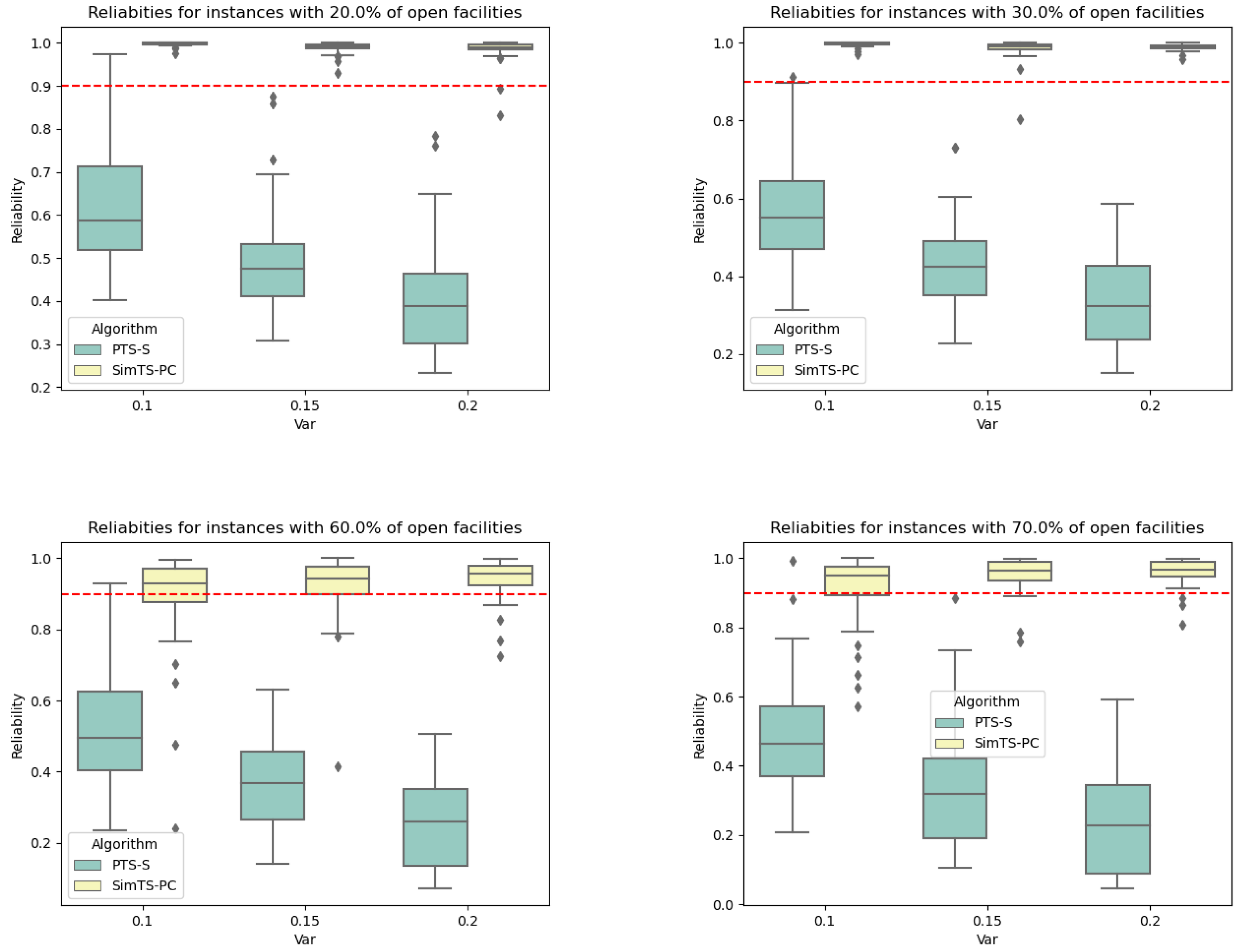
Yet another experiment is conducted to evaluate the effectiveness of the simheuristic under various configurations. To achieve this, we extend the instances by increasing the total required capacity, B, thereby compelling the algorithm to select more facilities. Figure 3 illustrates the reliability levels obtained with both the simheuristic and deterministic algorithms for different percentages of selected facilities (ranging from $20\%$ to $80\%$). It is evident that the simheuristic algorithm, SimTS-PC, consistently achieves the minimum required reliability of $0.90$ on average across all scenarios, outperforming the deterministic algorithm PTS, which exhibits reliability levels well below $0.9$ (highlighted in red in the diagrams). These results underscore the importance of considering stochasticity during the search process, as failure to do so can significantly impact the robustness of the final solution.

5.2. Numerical Experiments and Results for the SCDP-SC

Table 5. Performance of our algorithm for the SCDP-SC problem (4) with different variances.

Instance	$\mathit{\sigma }=0.1$							$\mathit{\sigma }=0.15$						$\mathit{\sigma }=0.2$
	PTS	PTS-S		SimTS-SC				PTS-S		SimTS-SC				PTS-S		SimTS-SC
	dist	dist	$\nu$	dist	$\nu$	dist-Gap		dist	$\nu$	dist	$\nu$	dist-Gap		dist	$\nu$	dist	$\nu$	dist-Gap
GKD-b_11_n50_b02_m5	147.2	84.27	0.57	136.84	0.95	−38.41%		74.73	0.50	139.18	0.97	−46.24%		70.22	0.47	130.61	0.91	−46.31%
GKD-b_12_n50_b02_m5	178.1	155.14	0.86	165.63	1.00	−6.33%		131.10	0.73	159.15	0.96	−17.14%		116.56	0.65	140.67	0.86	−17.62%
GKD-b_13_n50_b02_m5	96.1	60.68	0.63	89.99	0.98	−32.57%		54.04	0.56	82.15	0.89	−33.85%		49.36	0.51	74.63	0.85	−34.22%
GKD-b_14_n50_b02_m5	84.6	65.61	0.77	81.12	1.00	−19.12%		56.24	0.66	79.25	0.98	−32.26%		49.89	0.59	73.65	0.91	−29.04%
GKD-b_15_n50_b02_m5	154.9	113.81	0.73	146.06	0.95	−22.08%		97.78	0.63	137.36	0.93	−26.53%		86.52	0.55	117.76	0.80	−28.81%
GKD-b_16_n50_b02_m15	77.7	73.17	0.94	75.50	0.97	−3.09%		64.35	0.82	70.15	0.90	−3.79%		57.19	0.73	59.44	0.77	−8.28%
GKD-b_17_n50_b02_m15	41.8	22.10	0.53	34.78	0.95	−36.47%		20.51	0.49	34.06	0.97	−28.54%		19.04	0.45	26.65	0.73	−39.79%
GKD-b_18_n50_b02_m15	108.5	68.98	0.63	102.05	0.99	−32.40%		61.16	0.56	95.73	0.93	−33.13%		56.13	0.51	83.94	0.81	−36.11%
GKD-b_19_n50_b02_m15	119.1	116.03	0.97	114.80	0.96	1.07%		103.07	0.86	103.62	0.87	−0.03%		91.86	0.77	91.89	0.89	−0.53%
GKD-b_20_n50_b02_m15	115.3	59.78	0.51	111.48	1.00	−46.37%		55.38	0.48	107.46	0.96	−48.69%		51.69	0.44	100.75	0.90	−48.46%
GKD-b_41_n150_b02_m15	162.3	135.68	0.83	153.12	0.98	−11.39%		109.54	0.67	138.41	0.89	−24.23%		89.00	0.54	117.46	0.75	−20.86%
GKD-b_42_n150_b02_m15	84.3	45.36	0.53	73.22	0.98	−38.05%		40.29	0.47	67.06	0.89	−39.83%		34.52	0.40	57.38	0.76	−39.93%
GKD-b_43_n150_b02_m15	62	42.36	0.68	41.69	0.73	1.61%		34.46	0.55	34.59	0.61	2.13%		29.06	0.46	28.46	0.50	−0.37%
GKD-b_44_n150_b02_m15	101.6	62.15	0.60	92.66	0.94	−32.93%		51.84	0.50	79.40	0.80	−32.63%		45.29	0.44	67.22	0.68	−34.70%
GKD-b_45_n150_b02_m15	105.1	72.80	0.68	88.81	0.93	−18.03%		59.31	0.56	74.28	0.78	−22.06%		49.70	0.47	63.77	0.67	−20.16%
GKD-b_46_n150_b02_m45	123.8	52.65	0.42	107.57	0.92	−51.06%		48.38	0.38	101.49	0.91	−53.04%		42.09	0.33	89.63	0.80	−52.33%
GKD-b_47_n150_b02_m45	162.8	93.89	0.57	137.76	0.96	−31.85%		79.46	0.48	121.54	0.85	−33.21%		67.28	0.41	100.74	0.70	−34.62%
GKD-b_48_n150_b02_m45	99	46.58	0.46	70.59	0.72	−34.02%		40.62	0.40	64.75	0.73	−35.79%		35.31	0.35	54.99	0.62	−37.27%
GKD-b_49_n150_b02_m45	166.3	109.10	0.65	150.47	0.98	−27.50%		88.62	0.52	134.64	0.88	−34.13%		75.63	0.45	114.81	0.75	−34.18%
GKD-b_50_n150_b02_m45	110.1	54.90	0.49	91.56	0.97	−40.04%		46.38	0.41	80.82	0.86	−39.30%		42.49	0.38	69.99	0.74	−42.62%
MDG-b_01_n500_b02_m50	56.9	25.38	0.45	25.01	0.76	1.45%		19.24	0.34	25.14	0.55	−14.88%		15.59	0.29	18.32	0.40	−23.50%
MDG-b_02_n500_b02_m50	46.3	33.51	0.69	29.33	0.71	14.24%		25.23	0.52	21.58	0.50	12.77%		18.29	0.38	16.22	0.37	16.90%
MDG-b_03_n500_b02_m50	47.5	16.58	0.32	30.81	0.71	−46.19%		13.40	0.26	23.21	0.55	−43.50%		10.04	0.20	17.77	0.42	−42.26%
MDG-b_04_n500_b02_m50	46.7	21.94	0.44	37.08	0.78	−40.85%		15.56	0.31	23.89	0.47	−43.83%		12.09	0.24	21.52	0.46	−34.88%
MDG-b_05_n500_b02_m50	47.5	41.46	0.83	30.77	0.78	34.74%		30.70	0.62	22.37	0.57	32.67%		23.17	0.47	17.46	0.46	37.23%
MDG-b_06_n500_b02_m50	45.2	25.26	0.52	36.58	0.84	−30.95%		18.57	0.38	25.97	0.60	−28.73%		13.80	0.29	19.36	0.45	−28.51%
MDG-b_07_n500_b02_m50	44.9	26.81	0.55	32.72	0.77	−18.05%		20.30	0.42	23.57	0.56	−9.78%		15.34	0.32	17.00	0.40	−13.88%
MDG-b_08_n500_b02_m50	50.1	28.45	0.53	38.06	0.88	−25.25%		20.12	0.38	28.23	0.65	−30.24%		14.75	0.28	21.14	0.49	−28.74%
MDG-b_09_n500_b02_m50	50.7	34.89	0.66	39.75	0.80	−12.21%		25.50	0.48	26.04	0.60	−4.07%		18.28	0.35	19.05	0.44	−2.08%
MDG-b_10_n500_b02_m50	47	29.48	0.60	29.52	0.67	−0.15%		21.26	0.43	20.59	0.47	9.44%		16.14	0.33	14.75	0.34	3.24%
GKD-c_01_n500_b02_m50	9.1	7.09	0.62	7.42	0.82	−4.35%		5.04	0.44	5.39	0.61	−9.30%		3.65	0.32	4.02	0.46	−6.52%
GKD-c_02_n500_b02_m50	9.2	7.97	0.69	6.91	0.77	15.37%		5.78	0.50	5.16	0.57	17.81%		4.40	0.39	3.74	0.42	11.98%
GKD-c_03_n500_b02_m50	9.2	7.88	0.69	6.95	0.78	13.31%		5.83	0.51	5.04	0.58	−1.85%		4.25	0.37	4.33	0.42	15.64%
GKD-c_04_n500_b02_m50	9	4.74	0.39	6.88	0.76	−31.12%		3.55	0.30	5.10	0.49	−26.76%		2.68	0.22	3.66	0.35	−30.49%
GKD-c_05_n500_b02_m50	9	7.27	0.62	7.23	0.70	0.44%		5.02	0.44	5.27	0.52	0.33%		3.60	0.32	3.58	0.34	−4.61%
GKD-c_06_n500_b02_m50	9	7.45	0.66	6.80	0.76	9.55%		5.45	0.48	4.75	0.54	−6.09%		3.92	0.35	4.17	0.40	14.74%
GKD-c_07_n500_b02_m50	9	6.90	0.60	6.76	0.76	2.08%		5.07	0.45	6.22	0.62	−10.86%		3.67	0.32	4.12	0.47	−18.48%
GKD-c_08_n500_b02_m50	9.3	7.33	0.62	7.02	0.79	4.40%		5.22	0.45	6.17	0.69	−13.72%		3.70	0.32	4.29	0.49	−15.38%
GKD-c_09_n500_b02_m50	9	5.86	0.49	7.01	0.79	−16.49%		4.28	0.36	5.34	0.60	−18.89%		3.12	0.27	3.85	0.44	−19.89%
GKD-c_10_n500_b02_m50	9.1	8.61	0.78	7.24	0.80	18.80%		6.60	0.60	5.39	0.59	24.71%		4.87	0.44	3.90	0.43	22.46%
Average	71.86	47.25	0.62	61.64	0.86	−15.76%		39.47	0.50	54.99	0.72	−18.83%		33.85	0.41	47.17	0.60	−18.68%

presents the results for the SCDP-SC model, which aims to maximize the objective function. Similar to the previous table, the first column identifies the instance, while the subsequent columns display the obtained solutions for the three different variance levels tested. Each block includes the best deterministic solution evaluated under deterministic conditions with average values in the coefficient constraints (PTS), along with the associated expected cost evaluated under a stochastic scenario (PTS-S). Additionally, the table reports the reliability level associated with the stochastic solution. Each violation of the minimum capacity level incurs a penalty in the solution, as described in Section 3. The results in this table affirm the superiority of the simheuristic over its deterministic counterpart. Specifically, the objective function value (distance, $dist$) of the PTS heuristic evaluated in the deterministic problem is $71.86$. However, when evaluated in the stochastic problem, it decreases to $47.25$ due to its feasibility in only $62\%$ of the cases on average, as indicated in the reliability column ($\nu$). In the remaining cases, the solution is penalized by opening additional facilities. On the contrary, the SimTS-SC achieves an average objective value of $61.64$, attributable to its high reliability of $86\%$ on average. Similar results are observed for the other variance levels.

Table 6. Comparison of PTS-S and SimTS-SC categorized by type and instance size.

Size of the Instance (n)	$\mathit{\sigma }=0.1$			$\mathit{\sigma }=0.15$			$\mathit{\sigma }=0.2$
	dist PTS-S	dist SimTS-SC	dist-GAP	dist PTS-S	dist SimTS-SC	dist-GAP	dist PTS-S	dist SimTS-SC	dist-GAP
GKD   n = 50	81.96	105.83	−23.58%	71.84	100.81	−27.02%	64.85	90.00	−28.92%
GKD n = 150	71.55	100.75	−28.33%	59.89	89.70	−31.21%	51.04	76.45	−31.70%
MDG n = 500	7.11	7.02	1.20%	5.18	5.38	−4.46%	3.79	3.97	−3.06%
GKD n = 500	28.38	32.96	−12.32%	20.99	24.06	−12.02%	15.75	18.26	−11.65%

presents a summary of the objective function values categorized by type and instance size. Notice that, on average, the SimTS-SC algorithm outperforms the solutions obtained with PTS, exhibiting higher reliability, as observed in Table 5. Moreover, SimTS-SC demonstrates a superior performance in the Euclidean set of instances (GKD), contrasting with the MDG dataset, which features randomly generated distances.

As in the previous stochastic model, we evaluated our simheuristic for different demand levels, varying the aggregated demand from $0.2$ to $0.80$. Figure 4 illustrates the objective function value of both the deterministic and simheuristic algorithms. Across all the demand levels tested, the solution provided by our simheuristic consistently outperforms the simulated deterministic solutions (PTS-S). Overall, the results demonstrate that the solutions provided by our simheuristic significantly outperform the deterministic solutions when considered in a realistic scenario under uncertainty (PTS-S). It is evident that near-optimal solutions for the deterministic version of the problem may fall short in the stochastic version.

Carrying out a cross-analysis between both stochastic approaches, we can observe that the PTS-S algorithm provides solutions with higher reliabilities but lower objective function (OF) values than the PTS-S algorithm, which strives to maximize the OF values, leading to solutions with lower reliabilities. Note that the two models are complementary, and the decision-maker will choose between them based on their specific needs and requirements.

Finally, some statistical analyses have allowed us to ascertain the significance of the observed differences between both approaches. Given the non-parametric nature of our data, we employed the Wilcoxon signed-rank test, a robust non-parametric statistical hypothesis test, to compare pairs of dependent samples. The statistical analysis focused on assessing the performance of our SimTS algorithm against the PTS in both models of the problems (SC (3) and PC (4)) under varying levels of stochastic variance ($\sigma$ values of $0.1$, $0.15$, and $0.2$). For each variance level, we computed p-values to evaluate the null hypothesis that there is no difference in the median performance metrics between our simheuristic approach and the benchmarks. The open type values, like $0.2$ representing $20\%$ of nodes, indicate the fraction of nodes activated which have a feasible solution for each case. All p-values were significantly below the threshold of $\alpha =0.01$, leading us to reject the null hypothesis in each case. This indicates that the differences in performance metrics between our SimTS algorithm and PTS are statistically significant, with our approach demonstrating a superior solution quality and reliability under stochastic conditions (

Table 7. Wilcoxon test results comparing SimTS and PTS for each type of problem and variance level.

Model of the Problem	Open Type	Variance	Results
			Statistic	p-Value
SC (3)	0.2	0.1	0	$1.82\times {10}^{-12}$
		0.15	0	$1.82\times {10}^{-12}$
		0.2	0	$1.82\times {10}^{-12}$
	0.3	0.1	40	$1.58\times {10}^{-8}$
		0.15	0	$1.82\times {10}^{-12}$
		0.2	0	$1.82\times {10}^{-12}$
	0.6	0.1	0	$1.82\times {10}^{-12}$
		0.15	0	$1.82\times {10}^{-12}$
		0.2	0	$1.82\times {10}^{-12}$
	0.7	0.1	1	$3.64\times {10}^{-12}$
		0.15	0	$1.82\times {10}^{-12}$
		0.2	0	$1.82\times {10}^{-12}$
PC (4)	0.2	0.1	1036.5	0.00513
		0.15	182	$5.31\times {10}^{-12}$
		0.2	80	$1.41\times {10}^{-6}$
	0.3	0.1	165	$6.75\times {10}^{-4}$
		0.15	159	$4.79\times {10}^{-4}$
		0.2	166	$7.14\times {10}^{-4}$
	0.6	0.1	0	$1.82\times {10}^{-12}$
		0.15	0	$1.82\times {10}^{-12}$
		0.2	0	$1.82\times {10}^{-12}$
	0.7	0.1	7	$3.46\times {10}^{-11}$
		0.15	0	$1.82\times {10}^{-12}$
		0.2	0	$1.82\times {10}^{-12}$

).

6. Conclusions and Future Work

This paper analyzes two stochastic versions of the capacitated dispersion problem, in which a set of facilities is selected to provide a given service while maximizing their dispersion. In the first version, the aggregated capacity of the selected facilities must exceed the stochastic aggregated demand with a user-defined probability. Hence, the solutions need to be reliable to satisfy this probabilistic constraint. In the second version of the problem, the capacity requirement is modeled with a soft constraint, meaning that, when the aggregated capacity of the selected facilities does not cover the aggregated random demand, the solution is repaired and a penalty cost is added to the objective function to account for this failure.

In order to solve both versions of the stochastic CDPs, a simheuristic algorithm is proposed. In particular, its forward strategy starts with an empty solution and adds one ‘promising’ facility at a time until the aggregated capacity reaches a certain level; on the other hand, its backward strategy starts with all network facilities selected and removes one of them at each iteration until the minimum aggregate capacity is reached. The proposed simheuristic also benefits from a biased-randomization strategy, which can be seen as a special (and enhanced) version of a basic GRASP. The resulting hybrid metaheuristic performs remarkably well, as shown in the computational experiments. Specifically, our extensive experimentation demonstrates that our simheuristic algorithm is able to provide high-quality solutions to this NP-hard and stochastic optimization problem in short computational times compared with a competitive deterministic algorithm.

Several future directions can be considered at this point. Among them are the following: (i) modifying the current models to also consider non-stochastic uncertainty and then extending our approach into a fuzzy simheuristic one; (ii) employing stochastic programming methods, such as the sample average approximation, to highlight the advantages and drawbacks of simheuristic algorithms when compared with other simulation–optimization approaches; and (iii) extending this research to multi-objective optimization formulations. This work is an interdisciplinary piece of research, involving mathematics, computer science, and management science. The problem we address has direct applications in facility location problems but extends to a wide variety of real-life applications covering many fields, including biology and quantum computing, among others [7].

References

- Porumbel, D.C.; Hao, J.K.; Glover, F. A simple and effective algorithm for the MaxMin diversity problem. Ann. Oper. Res. 2011, 186, 275–293. [Google Scholar] [CrossRef]
- Wang, Y.; Hao, J.K.; Glover, F.; Lü, Z. A tabu search based memetic algorithm for the maximum diversity problem. Eng. Appl. Artif. Intell. 2014, 27, 103–114. [Google Scholar] [CrossRef]
- Pérez-Peló, S.; Sánchez-Oro, J.; Duarte, A. Greedy Randomized Adaptive Search Procedure. In Discrete Diversity and Dispersion Maximization: A Tutorial on Metaheuristic Optimization; Springer International Publishing: Cham, Switzerland, 2023; pp. 93–105. [Google Scholar]
- Kuby, M.J. Programming models for facility dispersion: The p-dispersion and maxisum dispersion problems. Math. Comput. Model. 1988, 10, 792. [Google Scholar] [CrossRef]
- Kuo, C.C.; Glover, F.; Dhir, K.S. Analyzing and Modeling the Maximum Diversity Problem by Zero-One Programming. Decis. Sci. 1993, 24, 1171–1185. [Google Scholar] [CrossRef]
- Dhir, K.; Glover, F.; Kuo, C.C. Optimizing diversity for engineering management. In Proceedings of the Engineering Management Society Conference on Managing Projects in a Borderless World, Washington, DC, USA, 17–18 December 1993; pp. 23–26. [Google Scholar]
- Martí, R.; Martínez-Gavara, A.; Pérez-Peló, S.; Sánchez-Oro, J. A review on discrete diversity and dispersion maximization from an OR perspective. Eur. J. Oper. Res. 2022, 299, 795–813. [Google Scholar] [CrossRef]
- Rosenkrantz, D.J.; Tayi, G.K.; Ravi, S.S. Facility Dispersion Problems under Capacity and Cost Constraints. J. Comb. Optim. 2000, 4, 7–33. [Google Scholar] [CrossRef]
- Erkut, E.; Neuman, S. Analytical models for locating undesirable facilities. Eur. J. Oper. Res. 1989, 40, 275–291. [Google Scholar] [CrossRef]
- Daskin, M.S. Network and Discrete Location: Models, Algorithms, and Applications; John Wiley & Sons: Hoboken, NJ, USA, 2011. [Google Scholar]
- Lu, Z.; Martínez-Gavara, A.; Hao, J.K.; Lai, X. Solution-based tabu search for the capacitated dispersion problem. Expert Syst. Appl. 2023, 223, 119856. [Google Scholar] [CrossRef]
- Chica, M.; Juan, A.A.; Bayliss, C.; Cordón, O.; Kelton, W.D. Why simheuristics? Benefits, limitations, and best practices when combining metaheuristics with simulation. SORT 2020, 44, 311–334. [Google Scholar] [CrossRef]
- Erkut, E. The discrete p-dispersion problem. Eur. J. Oper. Res. 1990, 46, 48–60. [Google Scholar] [CrossRef]
- Kincaid, R.K. Good solutions to discrete noxious location problems via metaheuristics. Ann. Oper. Res. 1992, 40, 265–281. [Google Scholar] [CrossRef]
- Glover, F.; Kuo, C.C.; Dhir, K.S. A discrete optimization model for preserving biological diversity. Appl. Math. Model. 1995, 19, 696–701. [Google Scholar] [CrossRef]
- Ağca, S.; Eksioglu, B.; Ghosh, J.B. Lagrangian solution of maximum dispersion problems. Nav. Res. Logist. 2000, 47, 97–114. [Google Scholar] [CrossRef]
- Chandra, B.; Halldórsson, M.M. Approximation Algorithms for Dispersion Problems. J. Algorithms 2001, 38, 438–465. [Google Scholar] [CrossRef]
- Silva, G.C.; Ochi, L.S.; Martins, S.L. Experimental comparison of greedy randomized adaptive search procedures for the maximum diversity problem. In Lecture Notes in Computer Science (Including Subseries Lecture Notes in Artificial Intelligence and Lecture Notes in Bioinformatics); Springer: Berlin/Heidelberg, Germany, 2004; Volume 3059, pp. 498–512. [Google Scholar]
- Aringhieri, R.; Cordone, R. Better and Faster Solutions for the Maximum Diversity Problem; Technical Report April; Université degli Studi di Milano, Polo Didattico e di Ricerca di Crema: Milano, Italy, 2006. [Google Scholar]
- Katayama, K.; Narihisa, H. An Evolutionary Approach for the Maximum Diversity Problem. In Recent Advances in Memetic Algorithms; Springer: Berlin/Heidelberg, Germany, 2006; pp. 31–47. [Google Scholar]
- Duarte, A.; Martí, R. Tabu search and GRASP for the maximum diversity problem. Eur. J. Oper. Res. 2007, 178, 71–84. [Google Scholar] [CrossRef]
- Palubeckis, G. Iterated tabu search for the maximum diversity problem. Appl. Math. Comput. 2007, 189, 371–383. [Google Scholar] [CrossRef]
- Wang, J.; Zhou, Y.; Cai, Y.; Yin, J. Learnable tabu search guided by estimation of distribution for maximum diversity problems. Soft Comput. 2012, 16, 711–728. [Google Scholar] [CrossRef]
- Zhou, Y.; Hao, J.K.; Duval, B. Opposition-based memetic search for the maximum diversity problem. IEEE Trans. Evol. Comput. 2017, 21, 731–745. [Google Scholar] [CrossRef]
- Brimberg, J.; Mladenović, N.; Todosijević, R.; Urošević, D. Less is more: Solving the Max-Mean diversity problem with variable neighborhood search. Inf. Sci. 2017, 382–383, 179–200. [Google Scholar] [CrossRef]
- De Freitas, A.; Guimarães, F.; Pedrosa Silva, R.; Souza, M. Memetic self-adaptive evolution strategies applied to the maximum diversity problem. Optim. Lett. 2014, 8, 705–714. [Google Scholar] [CrossRef]
- Prokopyev, O.A.; Kong, N.; Martinez-Torres, D.L. The equitable dispersion problem. Eur. J. Oper. Res. 2009, 197, 59–67. [Google Scholar] [CrossRef]
- Peiró, J.; Jiménez, I.; Laguardia, J.; Martí, R. Heuristics for the capacitated dispersion problem. Int. Trans. Oper. Res. 2021, 28, 119–141. [Google Scholar] [CrossRef]
- de Andrade, M.R.Q.; de Andrade, P.M.F.; Martins, S.L.; Plastino, A. GRASP with path-relinking for the maximum diversity problem. In Lecture Notes in Computer Science (Including Subseries Lecture Notes in Artificial Intelligence and Lecture Notes in Bioinformatics); Springer: Berlin/Heidelberg, Germany, 2005; pp. 558–569. [Google Scholar]
- Glover, F.; Laguna, M. Tabu Search. In Handbook of Combinatorial Optimization; Springer: Berlin/Heidelberg, Germany, 1998; pp. 2093–2229. [Google Scholar]
- Martí, R.; Martínez-Gavara, A.; Sánchez-Oro, J. The capacitated dispersion problem: An optimization model and a memetic algorithm. Memetic Comput. 2021, 13, 131–146. [Google Scholar] [CrossRef]
- Sayyady, F.; Fathi, Y. An integer programming approach for solving the p-dispersion problem. Eur. J. Oper. Res. 2016, 253, 216–225. [Google Scholar] [CrossRef]
- Glover, F. Scatter search and path relinking. New Ideas Optim. 1999, 138, 297–316. [Google Scholar]
- Mladenović, N.; Todosijević, R.; Urošević, D.; Ratli, M. Solving the Capacitated Dispersion Problem with variable neighborhood search approaches: From basic to skewed VNS. Comput. Oper. Res. 2022, 139, 105622. [Google Scholar] [CrossRef]
- Gomez, J.F.; Panadero, J.; Tordecilla, R.D.; Castaneda, J.; Juan, A.A. A multi-start biased-randomized algorithm for the capacitated dispersion problem. Mathematics 2022, 10, 2405. [Google Scholar] [CrossRef]
- Jucker, J.V.; Carlson, R.C. The Simple Plant-Location Problem under Uncertainty. Oper. Res. 1976, 24, 1045–1055. [Google Scholar] [CrossRef]
- Hodder, J.E.; Jucker, J.V. A simple plant-location model for quantity-setting firms subject to price uncertainty. Eur. J. Oper. Res. 1985, 21, 39–46. [Google Scholar] [CrossRef]
- Drezner, Z. Heuristic Solution Methods for Two Location Problems with Unreliable Facilities. J. Oper. Res. Soc. 1987, 38, 509–514. [Google Scholar] [CrossRef]
- Wang, Q.; Batta, R.; Rump, C.M. Algorithms for a facility location problem with stochastic customer demand and immobile servers. Ann. Oper. Res. 2002, 111, 17–34. [Google Scholar] [CrossRef]
- Ravi, R.; Sinha, A. Hedging uncertainty: Approximation algorithms for stochastic optimization problems. In Integer Programming and Combinatorial Optimization: 10th International IPCO Conference, New York, NY, USA, 7–11 June 2004, Proceedings; Bienstock, D., Nemhauser, G., Eds.; Springer: Berlin/Heidelberg, Germany, 2004; pp. 101–115. [Google Scholar]
- Snyder, L.V. Facility location under uncertainty: A review. IIE Trans. 2006, 38, 547–564. [Google Scholar] [CrossRef]
- Baron, O.; Berman, O.; Krass, D. Facility Location with Stochastic Demand and Constraints on Waiting Time. Manuf. Serv. Oper. Manag. 2008, 10, 484–505. [Google Scholar] [CrossRef]
- Wagner, M.R.; Bhadury, J.; Peng, S. Risk management in uncapacitated facility location models with random demands. Comput. Oper. Res. 2009, 36, 1002–1011. [Google Scholar] [CrossRef]
- Verma, A.; Verma, R.; Mahanti, N. A new approach to fuzzy uncapacitated facility location problem. Int. J. Soft Comput. 2010, 5, 149–154. [Google Scholar] [CrossRef]
- Contreras, I.; Cordeau, J.F.; Laporte, G. Stochastic uncapacitated hub location. Eur. J. Oper. Res. 2011, 212, 518–528. [Google Scholar] [CrossRef]
- Arabani, A.B.; Farahani, R.Z. Facility location dynamics: An overview of classifications and applications. Comput. Ind. Eng. 2012, 62, 408–420. [Google Scholar] [CrossRef]
- Correia, I.; da Gama, F.S. Facility location under uncertainty. In Location Science; Laporte, G., Nickel, S., Saldanha da Gama, F., Eds.; Springer International Publishing: Cham, Switzerland, 2015; pp. 177–203. [Google Scholar]
- Lu, M.; Ran, L.; Shen, Z.J. Reliable facility location design under uncertain correlated disruptions. Manuf. Serv. Oper. Manag. 2015, 17, 445–455. [Google Scholar] [CrossRef]
- Kim, D.; Lee, K.; Moon, I. Stochastic facility location model for drones considering uncertain flight distance. Ann. Oper. Res. 2019, 283, 1283–1302. [Google Scholar] [CrossRef]
- Abensur, E.O.; da Silva Paes, A.; Reyann Kasai Yamada, E.; Ruggieri, V.; Alves de Aquino, W. Stochastic facility location problem in a competitive situation: A game theory model for emergency financial services. Cogent Eng. 2020, 7, 1837411. [Google Scholar] [CrossRef]
- Parragh, S.N.; Tricoire, F.; Gutjahr, W.J. A branch-and-Benders-cut algorithm for a bi-objective stochastic facility location problem. OR Spectr. 2021, 44, 419–459. [Google Scholar] [CrossRef] [PubMed]
- Turkeš, R.; Sörensen, K.; Cuervo, D.P. A matheuristic for the stochastic facility location problem. J. Heuristics 2021, 27, 649–694. [Google Scholar] [CrossRef]
- Li, Y.; Li, X.; Shu, J.; Song, M.; Zhang, K. A General Model and Efficient Algorithms for Reliable Facility Location Problem Under Uncertain Disruptions. Informs J. Comput. 2022, 34, 407–426. [Google Scholar] [CrossRef]
- Lozano, M.; Rodríguez, F.J. Iterated Greedy. In Discrete Diversity and Dispersion Maximization: A Tutorial on Metaheuristic Optimization; Springer International Publishing: Cham, Switzerland, 2023; pp. 107–133. [Google Scholar]
- Canellas de Oliveira, E.; de Lima Martins, S.; Plastino, A.; Rosseti, I.; Silva, G.C.d. Data Mining in Heuristic Search. In Discrete Diversity and Dispersion Maximization: A Tutorial on Metaheuristic Optimization; Springer International Publishing: Cham, Switzerland, 2023; pp. 301–321. [Google Scholar]
- Aringhieri, R.; Cordone, R.; Melzani, Y. An Ant Colony Optimization approach to the maximum diversity problem. Note Del Polo 2007, 109, 1–24. [Google Scholar]
- Aghakhani, S.; Pourmand, P.; Zarreh, M. A mathematical optimization model for the pharmaceutical waste location-routing problem using genetic algorithm and particle swarm optimization. Math. Probl. Eng. 2023, 2023, 6165495. [Google Scholar] [CrossRef]
- Aringhieri, R.; Cordone, R.; Guastalla, A.; Grosso, A. Constructive and Destructive Methods in Heuristic Search. In Discrete Diversity and Dispersion Maximization: A Tutorial on Metaheuristic Optimization; Springer: Berlin/Heidelberg, Germany, 2023; pp. 65–91. [Google Scholar]
- Glover, F.; Kuo, C.C.; Dhir, K.S. Heuristic algorithms for the maximum diversity problem. J. Inf. Optim. Sci. 1998, 19, 109–132. [Google Scholar] [CrossRef]
- Spall, J.C. Introduction to Stochastic Search and Optimization: Estimation, Simulation, and Control; John Wiley & Sons: Hoboken, NJ, USA, 2005; Volume 65. [Google Scholar]
- Andradóttir, S. A global search method for discrete stochastic optimization. Siam J. Optim. 1996, 6, 513–530. [Google Scholar] [CrossRef]
- Villarinho, P.A.; Panadero, J.; Pessoa, L.S.; Juan, A.A.; Oliveira, F.L.C. A simheuristic algorithm for the stochastic permutation flow-shop problem with delivery dates and cumulative payoffs. Int. Trans. Oper. Res. 2021, 28, 716–737. [Google Scholar] [CrossRef]
- do C. Martins, L.; Hirsch, P.; Juan, A.A. Agile optimization of a two-echelon vehicle routing problem with pickup and delivery. Int. Trans. Oper. Res. 2021, 28, 201–221. [Google Scholar] [CrossRef]
Figure 1.
Example of a franchise location problem.
Figure 2.
Comparison between PTS and SimTS.
Figure 3.
Reliability box-plot comparing SimTS-PC with PTS-S.
Figure 4.
Objective function value (minimum distance) box-plot comparing SimTS-SC with PTS-S.