Magnetic Filaments: Formation, Stability, and Feedback

Abstract

As is well known, magnetic fields in space are distributed very inhomogeneously. Sometimes, field distributions have forms of filaments with high magnetic field values. As many observations show, such a filamentation takes place in convective cells in the Sun and other astrophysical objects. This effect is associated with the frozenness of the magnetic field into a medium with high conductivity that leads to the compression of magnetic field lines and formation of magnetic filaments. We analytically show, based on the general analysis, that the magnetic field intensifies in the regions of downward flows in both two-dimensional and three-dimensional convective cells. These regions of the hyperbolic type in magnetic fields play the role of a specific attractor. This analysis was confirmed by numerical simulations of 2D roll-type convective cells. Without dissipation, the magnetic field grows exponentially in time and does not depend on the aspect ratio between the horizontal and vertical scales of the cell. An increase due to compression in the magnetic field of highly conductive plasma is saturated due to the natural limitation associated with dissipative effects when the maximum magnitude of a magnetic field is of the order of the root of the magnetic Reynolds number Re_m. For the solar convective zone, the mean kinetic energy density exceeds the mean magnetic energy density for at least two orders of magnitude, which allows one to use the kinematic approximation of the MHD induction equation. In this paper, based on the stability analysis, we explain why downward flows influence magnetic filaments, making them flatter with orientation along the interfaces between convective cells.

1. Introduction

The phenomenon of collapse plays a significant role in terms of understanding how turbulence, convection, and other similar phenomena operate in fluids. Collapse is understood as a process of formation of singularities in a finite time for smooth initial conditions. Such processes have been widely studied for quite a long time. According to the classical concepts of the Kolmogorov–Obukhov theory [1,2] in the case of a low-viscosity limit, the vorticity fluctuations in the inertial interval with a scale $\lambda$ behave proportionally to ${\lambda }^{-2/3}$. This means that in the limit of small $\lambda$, we will have infinite amplitudes of fluctuations, which may indicate that classical turbulence is closely related to the occurrence of collapse. At the same time, when the highly accurate numerical modeling of such problems became possible, it turned out that collapse was in fact not observed in such cases [3] (see also the review paper [4] devoted to this subject). Nevertheless, the tendency for vorticity enhancement remains, but without blow-up behavior. At the same time, for two-dimensional hydrodynamics in the ideal case, solutions associated with collapse are forbidden [5,6,7]. In the 2D case, however, this does not exclude the existence of infinite exponential growth [8]. In 3D hydrodynamics, the generation of pancake-type structures was numerically observed when pancake thickness decreases with time according to an exponential law due to the compressible character of the vorticity field [9]. It is important to note that the appearance of such structures in a three-dimensional case is associated with the vorticity frozenness of a fluid [10]. It should be noted that in two-dimensional ideal flows, the vorticity rotor (called divorticity) is also a frozen vector field [8]. This means that not only vorticity, but also any other fields frozen into a medium, should be compressible, and all the arguments about collapse given above are applicable to them. The compressible feature of such fields is a sequence of their frozenness.

Another classical example of frozen fields is a magnetic field in the ideal magnetohydrodynamics (MHD) [11]. In this case, we may expect that the magnetic field should evolve by the same laws as the vorticity in ideal fluids and, consequently, compress into localized magnetic structures [12]. But, unlike fluids, the MHD operates with two vector fields, namely, velocity and magnetic field. If the kinetic energy density sufficiently exceeds the magnetic energy density, we can consider the evolution of the magnetic field in a given velocity distribution and ignore the influence of the growing magnetic field on velocity flows. Such a situation is realized in the convective zone of the Sun, where the ratio between mean kinetic energy density and magnetic pressure consists of at least two orders of magnitude. Indeed, in this case, the sizes of magnetic distributions have a tendency to decrease exponentially in time with exponential increases in the magnetic field values. The amplification of a magnetic field is a direct consequence of its frozenness.

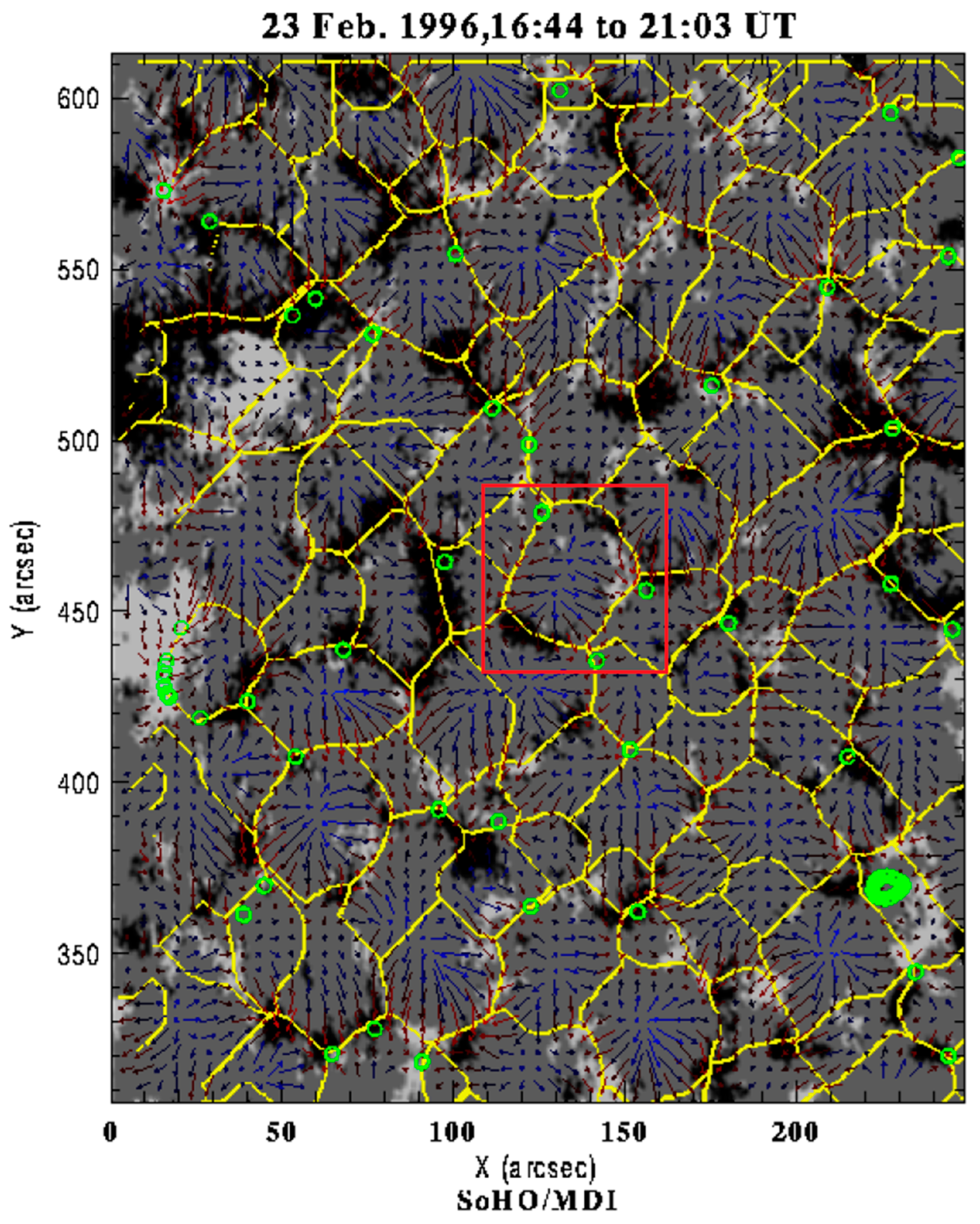
From the astrophysical point of view, the process of appearance of localized strong magnetic fields is of great interest. Thus, for the first time, Parker drew attention to the fact that the magnetic field in the convective zone of the Sun is noticeably filamented [13]. He studied magnetic field evolution in the case of a two-dimensional velocity field corresponding to convective rolls and showed exponential in time generation of magnetic filaments. Subsequently, these ideas were developed in many other works on this topic (see, [14,15,16,17,18,19,20,21,22,23,24,25] and references therein). According to the data of the Solar and Heliospherical Observatory (SOHO), in the convective zone of the Sun, filaments, in their majority, are concentrated near interfaces between convective cells and oriented correspondingly to downward flows [26]. The SOHO observations also show that filaments are almost absent at the centers of cells (Figure 1 and Figure 2).

An exponential increase in the magnetic field of the regions of downward flows follows from the topological arguments based on the Okubo–Weiss criteria [27,28]. These criteria divide flow area by hyperbolic and elliptic parts. Downward flows belong to hyperbolic regions. Due to the frozenness of the magnetic field into plasma, these regions play the roles of specific attractors. In elliptic regions, magnetic fields demonstrate the formation of spiral structures. Accounting finite conductivity in the hyperbolic regions leads to saturation of a magnetic field’s growth up to values proportional to the root square of the magnetic Reynolds number ${\mathrm{Re}}_m$ [14].

It is worth noting that both observations and estimations show that in the convective zone of the Sun, mean kinetic energy is sufficiently large in comparison to magnetic energy, so we can use it for descriptions of the magnetic field dynamics according to the MHD equations in kinematic approximation.

Note that the processes associated with the influence of convective flows are no less important in other astrophysical objects, such as galaxies, accretion disks, etc. In the simplest case, they can be taken into account using averaged models with account of the helicity fluxes of the magnetic field. At the same time, it is necessary to consider the corresponding effects more accurately within the framework of numerically modeling flows in such objects.

Previously, we studied the basic features of magnetic field amplification in convective cells [29] as an example of roll-type simple flow within a two-dimensional model. It was shown both numerically and analytically that, indeed, in the vicinity of hyperbolic points of the flow, the magnetic field increases exponentially in time. In the ideal case (${\mathrm{Re}}_m\to \infty$), the field growth is not limited. For finite magnetic viscosity, this process saturates, which gives the resulting magnetic field values of the order of ${\mathrm{Re}}_m^{1/2}$. It is also worth noting that in [29], we analyzed the cells of a square shape, i.e., for equal horizontal and vertical cell sizes. In reality, such an assumption is unlikely to be realized. It should be thought that the vertical dimension is greater than the horizontal dimension. The fact is that the convective transfer of heat into the Sun extends, according to all estimates, to distances greater than the horizontal dimensions of the convective cells. The main thing is that we do not know is at what depths the transition from turbulent convection to the observed laminar convection occurs. In this regard, it is necessary to understand how the process of formation of magnetic filaments is affected by an increase in the vertical size of the cells.

At the same time, the question arises as to whether the process of filamentation can be limited by other mechanisms. It is evident that the kinematic approximation in [29] cannot be applied to study the feedback influence of the growing magnetic field on the flow itself. Note that such an approach is very popular and is used often in dynamo theory [30,31,32]. In the case of dynamo theory, the simplest methods of nonlinear saturation are often used, which require a separate study of the stability of stationary solutions. In our case, intensive magnetic fields lead to the emergence of a large Lorentz force in the vicinity of magnetic filaments. This changes the nature of the flow of the medium, which, according to Lentz’s rule, can lead to a weakening of growth and probably its complete stop. Nevertheless, in the vicinity of a stationary hyperbolic point, the main direction of the Lorentz force will be parallel to the top convection surface with a high degree of accuracy. This means that the influence of the magnetic field on the flow may be strong enough in comparison with simple estimations. However, all this needs additional verification, which is one of the main aims of this work.

In this work, we will show how the problem of the formation of magnetic filaments in the convective zone of the Sun can be qualitatively studied based only on an analysis of the dynamics of the free surface of convective cells, i.e., reducing the dimension of the problem. This makes it possible to explain the formation of magnetic filaments in the vicinity of the interfaces between convective cells, i.e., in areas of downward flows, which act as specific attractors of the magnetic field. The growth of the magnetic field in the filaments occurs due to the freezing of the field. It is important that this result does not depend on the specific structure of the convective cell. A numerical experiment confirms this analytical concept.

2. Parameters of Solar Convective Zone

First of all, we present the main parameters of the solar convective zone. According to observations, the horizontal size $L$ for convective cells consists of 500–1000 km. For the solar convective cells in this paper, we will keep the assumption that the ratio between such scales is of the same order of magnitude (but not infinitely large) as for laboratory convection [29] (see also [30]). For the solar convection zone kinetic energy density that is much larger than the magnetic energy density, $\frac{\rho {\upsilon }^2}{2}>>\frac{B^2}{8\pi }$ (their ratio is about 10³–10⁴), where $\rho$ is a mass density, $B$ is the magnetic field value, and $\overrightarrow{\upsilon }$ is a flow velocity that is locally incompressible, $\mathrm{div}\overrightarrow{\upsilon }=0$. Therefore, the fluid velocity in this case can be considered as a given vector field. This limit is known as a kinematic approximation, which is widely used in the dynamo problem. Also note that near the boundary of the convective zone with the photosphere (the beginning of the Sun atmosphere), the mass density $\rho$ there is about 10⁻⁵ g/cm³. The characteristic velocity $U$ for cells is about 500 m/s. Their mean magnetic field $B_0$ is about a few gauss (for estimate we will take $B_0=10 \mathrm{G}$).

Thus, the dynamics of the magnetic field in the convective zone can be analyzed within one equation of the MHD system, i.e., for the magnetic field this is the induction equation:

$$\frac{\partial \overrightarrow{B}}{\partial t}=\overrightarrow{\nabla }\times \left(\overrightarrow{\upsilon }\times \overrightarrow{B}\right)+\frac{1}{{\mathrm{Re}}_m}\Delta \overrightarrow{B}$$

(1)

with a given (independent of magnetic field) velocity distribution $\overrightarrow{\upsilon }$ satisfying incompressibility condition $\mathrm{div}\overrightarrow{\upsilon }=0$.

In this equation, ${\mathrm{Re}}_m=\frac{UL}{\eta }$ is the magnetic Reynolds number and $\eta =\frac{c^2}{4\pi \sigma }$ is the magnetic viscosity, where $c$ is the speed of light, and $\sigma$ is the conductivity. According to all known data (see, e.g., [19,20] and references there), the ${\mathrm{Re}}_m$ in convective cells is of the order ${10}^6,$ which allows one to neglect dissipation in Equation (1). Thus, in this approximation, the magnetic field $\overrightarrow{B}$ turns out to be the frozen-in-fluid vector field. The frozenness means that the magnetic field lines move due to the velocity component normal to the magnetic field direction. As follows from (1), in this case the parallel velocity component does not have influence on the motion of magnetic field lines.

3. Generation of Magnetic Filaments by Two-Dimensional Flows

In this section, firstly, a convective flow is considered to be two-dimensional (lies in the $xy$ plane), stationary, and periodic along horizontal coordinate $x$. Thus, the cells are supposed to be of the roll type, where flows in two neighboring cells have opposite rotations. The vertical coordinate of the cell lattice changes in the following interval: $0\le y\le h;$ $y=0$ corresponds to the upper boundary of the convective zone, and $h$ is its depth. This geometry of the convective flow means that the normal velocity component ${\upsilon }_y=0$ at $y=0,$ namely, we neglect any perturbations of the top convective plane. Hence, for the $y$ component of the magnetic field at $y=0,$ in accordance with Equation (1) and the incompressibility condition $\mathrm{div}\overrightarrow{\upsilon }=0,$ one can obtain the following equation:

$$\frac{\partial B_y}{\partial t}+{\upsilon }_x\frac{\partial B_y}{\partial x}=-B_y\frac{\partial {\upsilon }_x}{\partial x}+{\mathrm{Re}}_m^{-1}{\nabla }^2{B}_y$$

(2)

Note that this equation becomes autonomous at zeroth magnetic viscosity, namely:

$$\frac{\partial B_y}{\partial t}+{\upsilon }_x\frac{\partial B_y}{\partial x}=-B_y\frac{\partial {\upsilon }_x}{\partial x}.$$

(3)

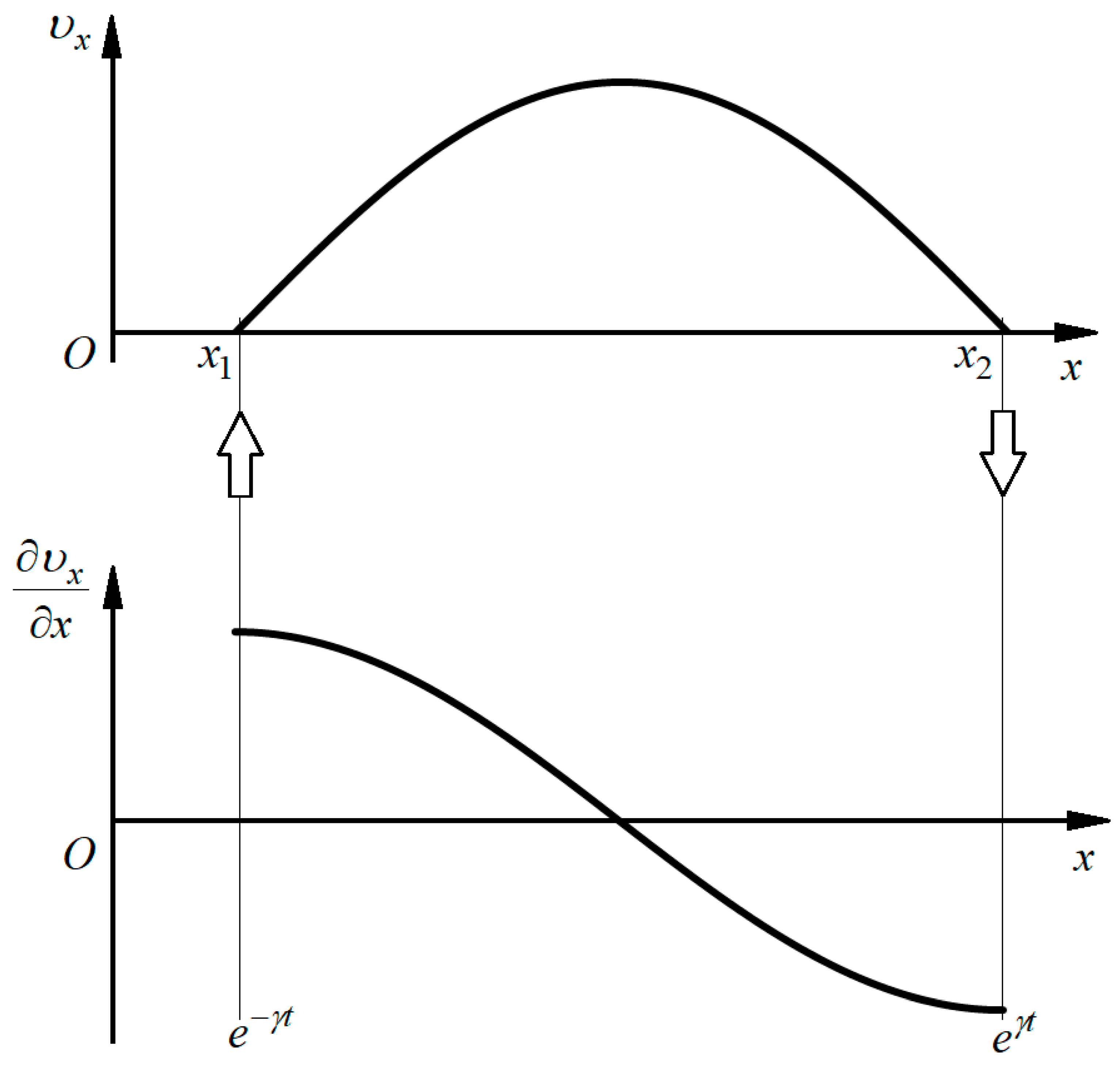
Consider the latter case in more detail. In a convection cell, the parallel velocity component ${\upsilon }_x$ at $y=0$ is equal to zero in the two points where convective flow makes turns of 90°. These points correspond to centers for upward and downward flows. Hence, it follows that the derivatives of ${\upsilon }_x$ in these points have different signs (Figure 3). At the center of upward flow, this derivative will be positive because this point ($x_1$) corresponds to flow source on the plane $y=0,$ but the second point ($x_2$) serves as a sink, and the derivative of ${\upsilon }_x$ will therefore be negative. Such behavior of the parallel velocity on the plane $y=0$ immediately shows that at the point with a positive derivative, B_y will decrease exponentially in time, $\propto \exp \left\{-{\left.\frac{\partial {\upsilon }_x}{\partial x}\right|}_{x=x_1}t\right\}$, and increase exponentially in the sink point, $x_2:$ $\propto \exp \left\{{\left.\frac{\partial {\upsilon }_x}{\partial x}\right|}_{x=x_2}t\right\}$. If the parallel velocity is symmetric (see Figure 3), then it is evident that decrement $\gamma \left(x_1\right)$ and increment $\gamma \left(x_2\right)$ will have the same values but opposite signs. Note that between these two points, as follows from Equation (3), besides amplification, the normal component of $\overrightarrow{B}$ undergoes advection towards point $x_2.$ Note that this motion is a consequence of the frozenness property of the magnetic field when the only the $\overrightarrow{B}$ component perpendicular to the convective flow undergoes advection.

Consider now what happens with another magnetic component. As we saw above, the behavior of the $B_y$ component at $y=0$ is based on both the stationary character of the convective flow and the assumption that the top convection boundary is planar. The same issue can be applied to the downward flow (plane $x=x_2$). Then, evidently the equation of motion for $B_x$ there will be analogous to (2):

$$\frac{\partial B_x}{\partial t}+{\upsilon }_y\frac{\partial B_x}{\partial y}=-B_x\frac{\partial {\upsilon }_y}{\partial y}.$$

(4)

Here, at $y=0$, the $x$-component of $\overrightarrow{\upsilon }$ will be equal to zero but its derivative at $x=x_2$ will be positive due to the incompressibility condition:

$$\frac{\partial {\upsilon }_y}{\partial y}=-\frac{\partial {\upsilon }_x}{\partial x}>0.$$

(5)

Hence, we have an exponential decrease in time of $B_x$ with maximal decrement:

$${\gamma }_{dis}=-{\left.\frac{\partial {\upsilon }_x}{\partial x}\right|}_{x=x_2,y=0}.$$

(6)

Thus, in the corner ($y=0,$ $x=x_2$), the magnetic field grows exponentially in time where the magnetic field direction is parallel to the downward flow and $\left|B_x\right|<<\left|B_y\right|$, respectively. Note that the point ($y=0,$ $x=x_2$) for this flow represents a hyperbolic point, respectively, and the region around this point belongs to the hyperbolic one in accordance with the Okubo–Weiss criterion (see below). Hence, using magnetic flux conservation it is possible to estimate the width $\delta$ of the forming magnetic filament:

$$〈{\left.B\right|}_{t=0}〉L\propto B_{\max }\delta .$$

(7)

Here, $〈{\left.B\right|}_{t=0}〉$ is the mean magnetic field and $L$ is the longitudinal size of the convective cell. This estimation indicates that the filament width compresses in time exponentially with decrement in ${\gamma }_{dis}$.

It is worth noting that the above analysis is general. It does not use a concrete structure of the convective cell. The only assumptions made are that the top convection surface is planar and the flow is stationary.

4. Numerical Simulations

In the numerics presented below, we show that these general conjectures are completely valid in the partial case of a convective flow of the roll type. Consider the flow of this type written in terms of stream function $\psi$:

$${\upsilon }_x=-\frac{\partial \psi }{\partial y};\hspace{1em}\hspace{1em}{\upsilon }_y=\frac{\partial \psi }{\partial x},$$

(8)

with the choice of $\psi$ in the form:

$$\psi \left(x,y\right)=V\sin k_{1}x\sin k_{2}y.$$

(9)

(Note that here, we use a different sign for stream function in comparison with the common definition, which is more convenient for us in numerics). Using dimensionless variables, it is convenient to take the values $V=\alpha ,$ $k_2=1/\alpha$, and $k_1=1$, where $\alpha$ is the aspect ratio and it characterizes the difference between the parallel and perpendicular sizes of the cell. In this case, the velocity takes the following form:

$${\upsilon }_x=-\sin x\cos \frac{y}{\alpha };$$

(10)

$${\upsilon }_y=\alpha \cos x\sin \frac{y}{\alpha }.$$

(11)

Note that at $y=0$, the $x$ velocity component is fixed and does not depend on aspect ratio $\alpha .$

We will consider the magnetic field $\overrightarrow{B}$ lying in the $xy$ plane. In this case, $\overrightarrow{B}$ can be expressed in terms of the $z$ component of the vector potential $\overrightarrow{A}=A{\overrightarrow{e}}_z$ as follows:

$$B_x=\frac{\partial A}{\partial y},\hspace{1em}\hspace{1em}{B}_y=-\frac{\partial A}{\partial x}.$$

(12)

Note that curves $A=\mathrm{const}$ coincide with the magnetic field lines.

We take the initial magnetic field $B_0$ constant in parallel to the $y$-axis, so that

$$A=-B_{0}x+a,$$

(13)

namely, ${\left.a\right|}_{t=0}=0$. In this case, induction Equation (1) in terms of potential a will be written as follows:

$$\frac{\partial a}{\partial t}+{\upsilon }_x\frac{\partial a}{\partial x}+{\upsilon }_y\frac{\partial a}{\partial y}=B_0{\upsilon }_x+\frac{1}{{\mathrm{Re}}_m}\Delta a.$$

(14)

We can solve this equation numerically for the periodic boundary condition relative to $x$: $a\left(\pi ,y\right)=a\left(-\pi ,y\right).$ As for the dependence of $a$ with respect to $y$, we also take the periodic boundary conditions’ continuing solution for a positive $y:$ $-\pi \alpha <y<+\pi \alpha .$

Equation (6) was solved numerically on the 2000 × 4000 grid $t_n=n\Delta t,$ $x_i=-\pi +i\cdot \Delta x,$ $y_j=-\pi +j\cdot \Delta y;$ using a simple numerical scheme [30]:

$$\begin{gathered} \frac{a_{i,j}^{n+1}-a_{i,j}^n}{\Delta t}+{\left({\upsilon }_x\right)}_{i,j}^n\frac{a_{i+1,j}^n-a_{i-1,j}^n}{2\Delta x}+{\left({\upsilon }_x\right)}_{i,j}^n\frac{a_{i,j+1}^n-a_{i,j-1}^n}{2\Delta y}= \\ =B_0{\left({\upsilon }_x\right)}_{i,j}^n+\frac{1}{{\mathrm{Re}}_m}\left(\frac{a_{i+1,j}^n-2a_{i,j}^n+a_{i-1,j}^n}{\Delta x^2}+\frac{a_{i,j-1}^n-2a_{i,j}^n+a_{i,j-1}^n}{\Delta y^2}\right) \end{gathered}$$

Such schemes are stable for time steps $\Delta t=O^{*}\left({\mathrm{Re}}_m\left(\Delta x^2+\Delta y^2\right)\right)$ [33]. Usually, we used $\Delta t=2.5\cdot {10}^{-5}$.

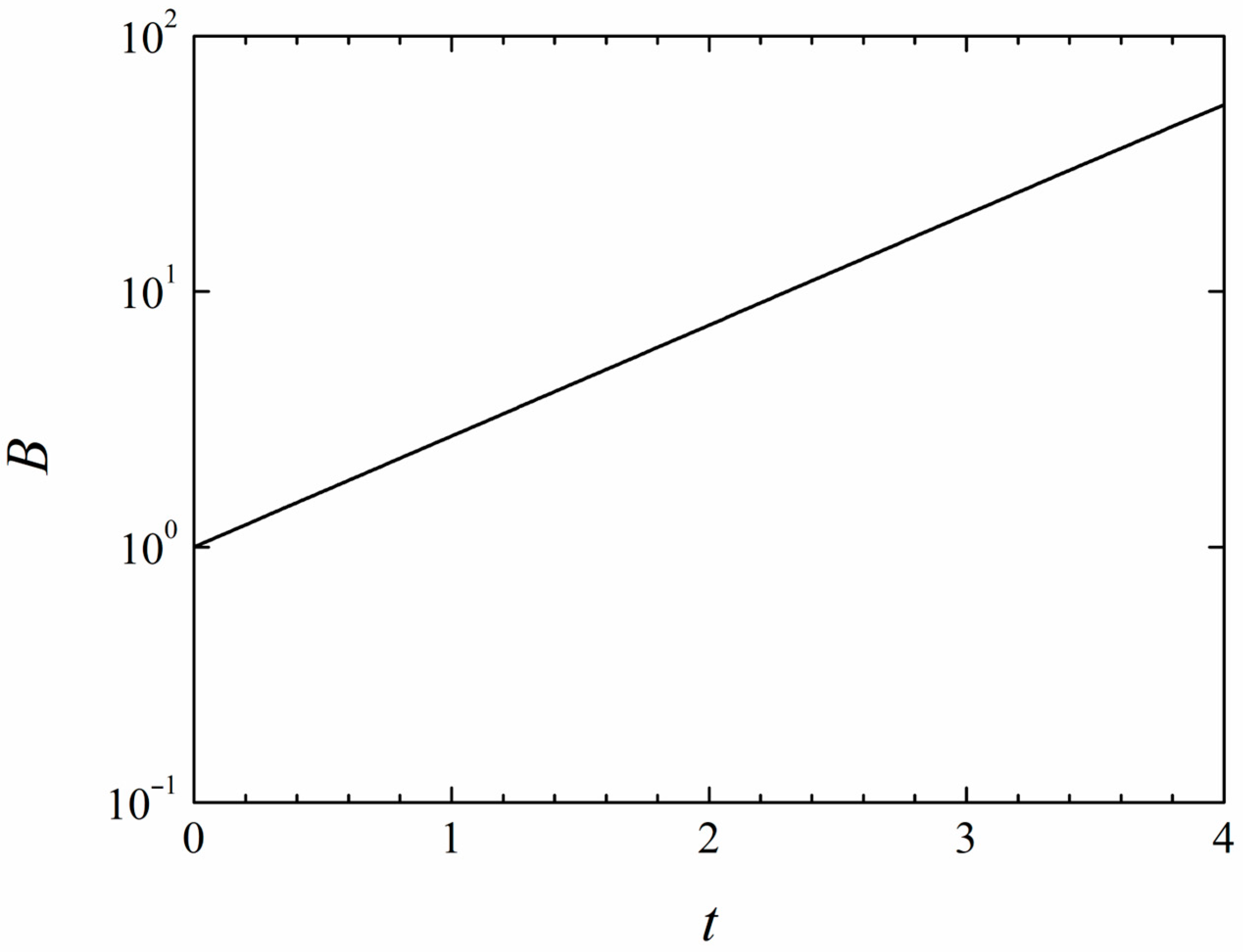
Now, we present the results of the numerical simulation of Equation (6) at ${\mathrm{Re}}_m=\infty .$ First of all, we have verified that the magnetic field grows exponentially with time in the hyperbolic region, which is defined in accordance with the Okubo–Weiss criterion [27,28]:

$${\psi }_{xx}{\psi }_{yy}-{\psi }_{xy}^2<0.$$

(15)

We have also observed that the magnetic field amplification in this region happens due to the frozenness property of the magnetic field into plasma. In this case, the maximum the growth rate is achieved in the corner $y=0,$ $x=0$, which corresponds to the stationary hyperbolic point coinciding with the centers of the downward flow (see, Figure 4). The magnetic field in this point is parallel to the downward convective flows. The vector potential A is shown in Figure 5 at t = 4.

We also checked that the maximal growth rate does not depend on the aspect ratio, in complete correspondence with the general consideration presented above (see previous section, when ${\mathrm{Re}}_m=\infty )$.

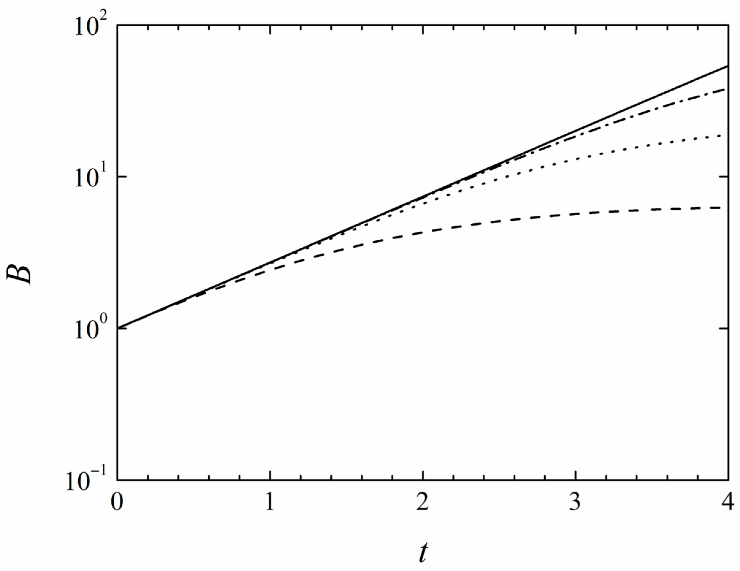
At a finite magnetic Reynolds number, conductivity leads to destruction of the field frozenness, which results in saturation of the exponential growth (see Figure 6).

At ${\mathrm{Re}}_m>>1$, it is possible to estimate the value of this field saturation in the magnetic filament. As was shown above, the $B_x$ component near the maximal point is a much smaller $B_y$ component that gives very different scales in the horizontal and vertical directions. This means that in Equation (3) for $B_y$, one can neglect the second derivative relative to $y$ in the Laplace operator and consider the velocity ${\upsilon }_x$ to be linearly dependent on $x-x_2$:

$$\frac{\partial B_y}{\partial t}-\frac{\partial }{\partial x}(x{B}_y)={\mathrm{Re}}_m^{-1}\frac{{\partial }^2{B}_y}{\partial x^2}$$

(16)

where we designate $x-x_2$ as $x$ and $V=1$. Saturation is reached at the stationary solution of this equation, which after integration gives the following:

$$B_y=B_{\max }\exp \left(-x^2{\mathrm{Re}}_m/2\right).$$

(17)

The value of $B_{\max }$ can be obtained using the magnetic field flux constancy. Approximately, $B_{\max }$ is equal to [29] the following:

$$B_{\max }=2.51B_0{\mathrm{Re}}_m^{1/2}.$$

(18)

According to [29], the width $\delta$ of this stationary filament was estimated as $L{\mathrm{Re}}_m^{-1/2}$.

5. Three-Dimensional Effects in Magnetic Filamentation

As we saw in the previous section for roll-type convection, the appearance of magnetic filaments takes place in a small vicinity at the stationary hyperbolic point $y=0,$ $x=x_2=0.$ In this region, the velocity in dimensionless variables can be written as follows: ${\upsilon }_x=-x$ and ${\upsilon }_y=y.$ When magnetic viscosity is small enough and its influence is not too essential, the $B_x$ component tends to zero exponentially in time but the $B_y$ component grows exponentially. The filaments in this case represent a special kind of attractor. Account of the finite magnetic viscosity leads to saturation of this growth and the formation of stationary filaments parallel to the downward flow. At ${\mathrm{Re}}_m>>1$, thus in the three-dimensional geometry, these filaments form the whole plane of the small width. Consider their stability relative to $z$ coordinate fluctuations, taking into account the $B_z$ component. At ${\mathrm{Re}}_m=\infty$, the equation for $B_z$ has the following form:

$$\frac{\partial B_z}{\partial t}+\left(\overrightarrow{\upsilon }\cdot \overrightarrow{\nabla }\right)B_z=0;$$

(19)

where the velocity has two components with ${\upsilon }_z=0.$ Thus, the $B_z$ component represents a passive scalar and can not change on the filaments. Moreover, the viscous term evidently provides its dissipation. Therefore, filaments in the three-dimensional case with planar downward flow have a tendency to be parallel to this surface.

However, the real situation, for instance, for solar cells, has some peculiarities different from those of the roll-type convection. This is already seen from the experimental data presented in Figure 1 and Figure 2.

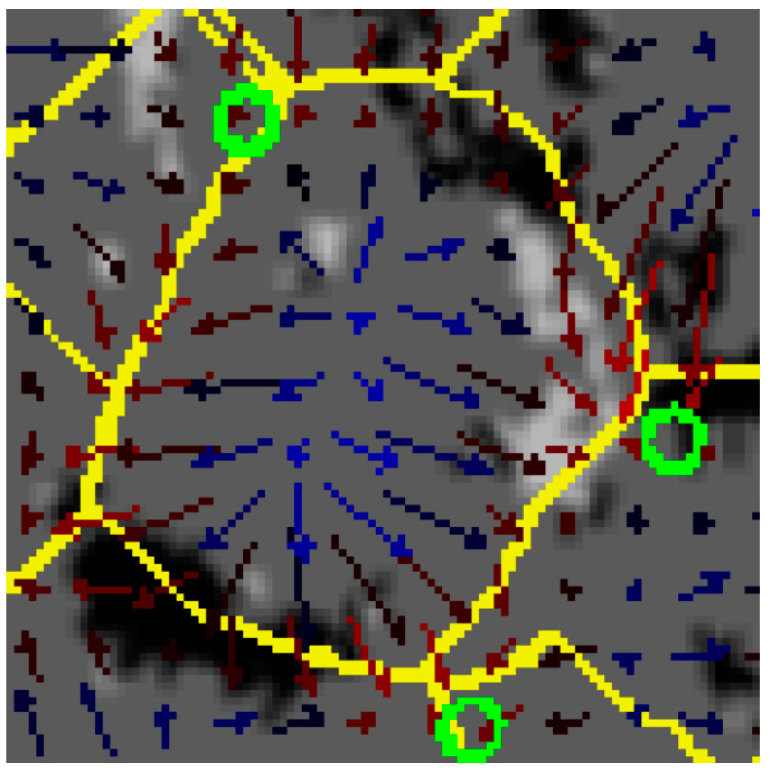
Firstly, solar filaments in the convective zone are concentrated in their majority near interfaces between convective cells and are oriented correspondingly to downward flows [26]. Secondly, filaments are rare at the centers of convective cells. The insets of Figure 1 and Figure 2 for a single cell shows such features in more detail.

We will give an explanation of these facts. First of all, a reminder that for the convective zone, ${\mathrm{Re}}_m$ is of the order ${10}^6$, which allows one to use the frozenness equation:

$$\frac{\partial \overrightarrow{B}}{\partial t}=\overrightarrow{\nabla }\times \left(\overrightarrow{\upsilon }\times \overrightarrow{B}\right).$$

(20)

It is not difficult to obtain that the projection of this equation on the top convective surface ($z=0$) gives the following equation of motion for the normal ($‖\widehat{z}$) component of $\overrightarrow{B}$:

$$\frac{\partial B_z}{\partial t}+\left({\overrightarrow{\upsilon }}_{\perp }\cdot \overrightarrow{\nabla }\right)B_z=-B_z\mathrm{div}{\overrightarrow{\upsilon }}_{\perp }.$$

(21)

This equation is derived by means of the incompressibility condition

$$\mathrm{div}{\overrightarrow{\upsilon }}_{\perp }+\frac{\partial {\upsilon }_z}{\partial z}=0$$

(22)

and using the boundary condition ${\upsilon }_z=0$ at $z=0.$ The latter means that surface $z=0$ is supposedly not deformed, as was considered in the 2D case. Therefore, Equation (21) represents an analogue of Equation (4). Then, by the same reason as before, at the flow source center $\overrightarrow{r}={\overrightarrow{r}}_0$, the perpendicular velocity component ${\overrightarrow{\upsilon }}_{\perp }$ is equal to zero but its divergence there will be a definite positive: $\mathrm{div}{\overrightarrow{\upsilon }}_{\perp }>0$. This provides the exponential decrease in time of the normal component $B_z$ at the cell source center. However, at the interface with a neighboring cell (this is the starting position of a downward flow), we have the opposite situation: the transverse velocity vanishes but its divergence there takes negative values. This means that component $B_z$ will grow exponentially in time at the interface. The growth rate $\gamma$ equal to $|\mathrm{div}{\overrightarrow{\upsilon }}_{\perp }|$ along the interface will be a function of its position. This means that some places at the interface will undergo bigger amplifications of $B_z$ than in another region of the interface. This inhomogeneity in the growth rate will cause filaments to form in regions of maximum enhancement while maintaining their orientation along the interface. As a result, the filaments will be quasi-flat as, for instance, is seen in Figure 2. Note also that amplification does not depend on the sign of the normal component $B_z:$ two kinds of filaments separated from each other are possible with different polarities in magnetic field (such a situation can only happen in the 3D case).

As in the 2D case, the second term in Equation (19) describes the advection of the $B_z$ component towards the interface.

Thus, in the kinematic approximation, we have two factors leading to the formation of filaments: advection and the exponential growth of filaments at the interface. This explains the experimental observations that solar filaments in the convective zone in their majority are concentrated near interfaces between convective cells and are oriented correspondingly to downward flows. As is seen from Figure 1 and Figure 2, magnetic filaments are rare at cell centers because of the advection of magnetic fields towards the periphery due to the frozenness property.

As for magnetic field values of filaments in the 3D case, they will have the same order of magnitude as in (18).

6. Feedback

Let us consider the Navier–Stokes equation in the presence of a magnetic field in the Boussinesq approximation

$$\frac{\partial \overrightarrow{\upsilon }}{\partial t}+\left(\overrightarrow{\upsilon }\cdot \overrightarrow{\nabla }\right)\overrightarrow{\upsilon }=-\overrightarrow{\nabla }p+\nu R_{a}T\overrightarrow{n}+\left[\left[\stackrel{\rightharpoonup }{\nabla }\times \stackrel{\rightharpoonup }{B}\right]\times \overrightarrow{B}\right]+\nu \Delta \overrightarrow{\upsilon },$$

(23)

where the magnetic field is written in Alfvenic units: $\overrightarrow{B}/\sqrt{4\pi \rho }\to \overrightarrow{B},$ i.e., has the dimension of speed, $R_a$ is the Rayleigh number, $T$ is the deviation of the temperature from its linear in $z$ dependence, $\overrightarrow{n}$—unit vector along the vertical $z,$ $\nu$—kinematic velocity, and $p$—pressure.

In this case, we will assume temperature fluctuation vanishes at the boundary $z=0:$ ${\left.T\right|}_{z=0}=0.$ Another boundary condition is written in the form of a continuity condition for the projection of the momentum flux density onto the normal:

$$\left\{{\sigma }_{ik}{n}_k\right\}=0,$$

(24)

where curly brackets mean a jump at $z=0,$ and

$${\sigma }_{ik}=-{\upsilon }_i{\upsilon }_k-\left(p+B^2/2\right){\delta }_{ik}+B_i{B}_k+\nu \left(\frac{\partial {\upsilon }_i}{\partial x_k}+\frac{\partial {\upsilon }_k}{\partial x_i}\right).$$

(25)

Since the surface $z=0$ is fixed, the first term in (25) after substitution into (24) drops out due to ${\left.{\upsilon }_z\right|}_{z=0}=0.$ It also follows that derivative ${\overrightarrow{\nabla }}_{\perp }{\upsilon }_z=0$ (where ${\overrightarrow{\nabla }}_{\perp }$ is the gradient along the surface $z=0$).

In the two-dimensional case, (24) implies two relations:

$$\left\{-B_x^2/2\right\}-p+2\nu \frac{\partial {\upsilon }_y}{\partial y}=0,$$

(26)

$$\left\{B_x\right\}{B}_y+\nu \frac{\partial {\upsilon }_x}{\partial y}=0.$$

(27)

In these expressions, we took into account the jump in the normal component of the magnetic field

$$\left\{B_y\right\}=0.$$

(28)

As we saw earlier, in the region of magnetic field filament formation in the case of high conductivity (${\mathrm{Re}}_m>>1$ [34]), component $\left|B_y\right|>>\left|B_x\right|$ at the boundary at $y=0.$ In this case, the relations of (26) and (27) at approximately $\nu \ne 0$ can be written as

$$-p+2\nu \frac{\partial {\upsilon }_y}{\partial y}=0,$$

(29)

$$\frac{\partial {\upsilon }_x}{\partial y}=0.$$

(30)

In this case, Equation (23) for ${\upsilon }_x$ at $y=0$ takes the form

$$\frac{\partial {\upsilon }_x}{\partial t}+{\upsilon }_x\frac{\partial }{\partial x}{\upsilon }_x=-B_y\frac{\partial }{\partial x}{B}_y+3\nu \frac{{\partial }^2}{\partial x^2}{\upsilon }_x+\nu \frac{{\partial }^2}{\partial y^2}{\upsilon }_x.$$

(31)

Far from filaments where $B_y\approx 0$, the convection flow should be independent of time, i.e., the last term in (31) can as such only provide a stationary flow. In this case, the ratio between inertial term and viscous one is of the order of the Reynolds number $\mathrm{Re}$. According to [32,34], it is of the order of 10². When we approach magnetic filaments, this ratio is assumed to be valid. The compensation of the inertial term (second term in (31)) is due to the gradient of magnetic pressure in filaments. Thus, the Hartmann number $\mathrm{Ha}$ defined as the ratio of electromagnetic force to the viscous force is of the order of the Reynolds number $\mathrm{Re}$.

In the special case of zero viscosity, the relations of (26) and (27) are also significantly simplified:

$$\begin{gathered} \left\{B_x\right\}=0, \\ p=0 \mathrm{at} y=0. \end{gathered}$$

(32)

From (26) and (27), it is also clear that for $\nu \to 0$, the longitudinal component of the magnetic field also turns out to be small.

Thus, on the surface $y=0$, with zero values of kinematic and magnetic viscosity, and neglecting the transverse component of the magnetic field $B_x$, the equation for the field velocity component ${\upsilon }_x$ and the components of the magnetic field $B_y$ turn out to be closed:

$$\frac{\partial {\upsilon }_x}{\partial t}+{\upsilon }_x\frac{\partial {\upsilon }_x}{\partial x}=-B_y\frac{\partial B_y}{\partial x},$$

(33)

$$\frac{\partial B_y}{\partial t}+{\upsilon }_x\frac{\partial B_y}{\partial x}=-B_y\frac{\partial {\upsilon }_x}{\partial x}.$$

(34)

It is easy to see that the sum and difference $w_x={\upsilon }_x\pm B_y$ obey two independent Hopf equations:

$$\frac{\partial w_{\pm }}{\partial t}+w_{\pm }\frac{\partial w_{\pm }}{\partial x}=0.$$

(35)

In the case of a convective zone, we must assume that at the initial moment the average kinetic energy density at $t=0$ significantly exceeds the magnetic energy density:

$$\frac{〈{\upsilon }_x^2〉}{2}>>\frac{B_0^2}{2}.$$

(36)

According to Equation (33), one can see that the growth in magnetic field $B$ due to the magnetic pressure gradient (the r.h.s. of (33)) prevents penetration of the flow in the hyperbolic region with its center at $y=0,$ $x=0.$ For this reason, the hyperbolic point will be moved towards the counter flow that provides an inverse influence on the growing magnetic field of the convective flow. Because the filament region is small in comparison to the convective cell, such a shift should not significantly influence the convection itself. It is evident that this mechanism shows that the magnetic pressure $B^2/2$ is comparable to the mean kinetic energy density $〈{\upsilon }^2〉/2$.

7. Conclusions

In this paper, we have analyzed the filamentation of the magnetic field in convective cells in the Sun within the kinematic approximation. This process is associated with the frozenness of the magnetic field into a medium with high conductivity, which leads to the compression of magnetic field lines and the formation magnetic filaments. Based on the general consideration of the convection top flows only, and without knowledge of the cell structure, we demonstrate that the magnetic field intensifies in the regions of downward flows in both two-dimensional and three-dimensional convective cells. These hyperbolic-type regions play the role of a specific attractor of the magnetic field. This theoretical analysis was confirmed by numerical simulations for 2D convective cells of the roll type. Without dissipation, the magnetic field grows exponentially in time and attains its maximal value at the hyperbolic point where the growth rate does not depend on the aspect ratio between the horizontal and vertical scales of the cell. This increase due to the compression of the magnetic filaments is saturated due to the natural limitation associated with finite plasma conductivity when the maximum magnitude of the magnetic field is of the order of the root square of the magnetic Reynolds number. Another effect of saturation of the magnetic field values is connected with feedback of the growing field on the convective flows. Both of these effects on the Sun convective zone give the maximal magnetic field values in filaments the same order of magnitude of about 1 kG. Based on the stability analysis, we have explained why downward flows influence magnetic filaments by making them flatter with orientation along the interfaces between convective cells.

References

- Kolmogorov, A. The Local Structure of Turbulence in Incompressible Viscous Fluid for Very Large Reynolds’ Numbers. Dokl. Akad. Nauk SSSR 1941, 30, 301–305. [Google Scholar]
- Obukhov, A.M. On the distribution of energy in the spectrum of turbulent flow. Dokl. Akad. Nauk SSSR 1941, 32, 136–139. [Google Scholar]
- Hou, T.Y.; Li, R. Computing nearly singular solutions using pseudo-spectral methods. J. Comput. Phys. 2007, 226, 379–397. [Google Scholar] [CrossRef]
- Gibbon, J.D. On the distribution of energy in the spectrum of turbulent flow. Phys. D Nonlinear Phenom. 2008, 237, 1894–1904. [Google Scholar] [CrossRef]
- Wolibner, W. Un theorème sur l’existence du mouvement plan d’un fluide parfait, homogène, incompressible, pendant un temps infiniment long. Math Z 1933, 37, 698–726. [Google Scholar] [CrossRef]
- Yudovich, V.I. Non-stationary flow of an ideal incompressible liquid. USSR Comput. Math. Math. Phys. 1963, 3, 1407–1456. [Google Scholar] [CrossRef]
- Kato, T. On classical solutions of the two-dimensional non-stationary Euler equation. Arch. Ration. Mech. Anal. 1967, 25, 188–200. [Google Scholar] [CrossRef]
- Kuznetsov, E.A.; Naulin, V.; Nielsen, A.H.; Rasmussen, J.J. Effects of sharp vorticity gradients in two-dimensional hydrodynamic turbulence. Phys. Fluids 2007, 19, 105110. [Google Scholar] [CrossRef]
- Agafontsev, D.S.; Kuznetsov, E.A.; Mailybaev, A.A.; Sereshchenko, E.V. Compressible vortical structures and their role in the hydrodynamical turbulence onset. Phys. Uspekhi 2022, 65, 189–208. [Google Scholar] [CrossRef]
- Kuznetsov, E.A.; Ruban, V.P. Hamiltonian dynamics of vortex lines in hydrodynamic-type systems. J. Exp. Theor. Phys. Lett. 1998, 67, 1076–1081. [Google Scholar] [CrossRef]
- Landau, L.D.; Lifshitz, E.M. Electrodynamics of Continuous Media; Pergamon Press: Oxford, UK, 1984. [Google Scholar]
- Kuznetsov, E.A.; Passot, T.; Sulem, P.L. Compressible dynamics of magnetic field lines for incompressible magnetohydrodynamic flows. Phys. Plasmas 2004, 11, 1410–1415. [Google Scholar] [CrossRef]
- Parker, E.N. Kinematical Hydromagnetic Theory and its Application to the Low Solar Photosphere. Astrophys. J. 1963, 138, 552–575. [Google Scholar] [CrossRef]
- Gelting, A.V. Convective Mechanism for the Formation of Photospheric Magnetic Fields. Astron. Rep. 2001, 45, 569–576. [Google Scholar]
- Stix, M. The Sun: An Introduction; Springer: Berlin, Germany, 2002. [Google Scholar]
- Galloway, D.J.; Weiss, N.O. Convection and magnetic field in stars. Astrophys. J. 1981, 243, 945–953. [Google Scholar] [CrossRef]
- Anzer, U.; Galloway, D.J. A model for the magnetic field above supergranules. Mon. Not. R. Astron. Soc. 1983, 203, 637–650. [Google Scholar] [CrossRef]
- Arter, W. Magnetic-flux transport by a convecting layer including dynamical effects. Geophys. Astrophys. Fluid Dyn. 1983, 31, 311–344. [Google Scholar] [CrossRef]
- Solanki, S.K. Sunspots: An overview. Astron. Astrophys. Rev. 2003, 11, 153–286. [Google Scholar] [CrossRef]
- Silvers, L.J. Evolution of zero-mean magnetic fields in cellular flows. Phys. Fluids 2005, 17, 103604. [Google Scholar] [CrossRef]
- Ferriz-Mas, A.; Steiner, O. How to Reach Superequipartition Field Strengths in Solar Magnetic Flux Tubes. Sol. Phys. 2007, 246, 31–39. [Google Scholar] [CrossRef]
- Nagata, S.; Tsuneta, S.; Suematsu, Y.; Ichimoto, K.; Katsukawa, Y.; Shimizu, T.; Yokoyama, T.; Tarbell, T.D.; Lites, B.W.; Shine, R.A.; et al. Formation of Solar Magnetic Flux Tubes with Kilogauss Field Strength Induced by Convective Instability. Astrophys. J. Lett. 2008, 677, L145. [Google Scholar] [CrossRef]
- Kitiashvili, I.N.; Kosovichev, A.G.; Wray, A.A.; Mansour, N.N. Mechanism of Spontaneous Formation of Stable Magnetic Structures on the Sun. Astrophys. J. 2010, 719, 307–312. [Google Scholar] [CrossRef]
- Tiwarui, S.K.; van Noort, M.; Lagg, A.; Solanki, S.K. Structure of sunspot penumbral filaments: A remarkable uniformity of properties. Astron. Astrophys. 2013, 557, A25. [Google Scholar] [CrossRef]
- Ryutova, M. Physics of Magnetic Flux Tubes; Springer: Berlin, Germany, 2018. [Google Scholar]
- Available online: https://sohowww.nascom.nasa.gov/ (accessed on 27 November 2023).
- Okubo, A. Horizontal dispersion of floatable particles in the vicinity of velocity singularities such as convergences. Deep Sea Res. Oceanogr. Abstr. 1970, 17, 445–454. [Google Scholar] [CrossRef]
- Weiss, J. The dynamics of enstrophy transfer in two-dimensional hydrodynamics. Phys. D Nonlinear Phenom. 1991, 48, 274–294. [Google Scholar] [CrossRef]
- Kuznetsov, E.A.; Mikhailov, E.A. Notes on Collapse in Magnetic Hydrodynamics. J. Exp. Theor. Phys. 2020, 131, 496–505. [Google Scholar] [CrossRef]
- Molchanov, S.A.; Ruzmajkin, A.A.; Sokolov, D.D. The kinematic dynamo in a random flux. Sov. Phys. Uspekhi 1985, 28, 307–327. [Google Scholar] [CrossRef]
- Chertkov, M.; Falkovich, G.; Kolokolov, I.; Vergassola, M. Small-Scale Turbulent Dynamo. Phys. Rev. Lett. 1999, 83, 4065–4068. [Google Scholar] [CrossRef]
- Sokoloff, D.D. Problems of magnetic dynamo. Phys. Uspekhi 2015, 58, 601–605. [Google Scholar] [CrossRef]
- Kalitkin, N.N. Numerical Methods; Nauka: Moscow, Russia, 1978. [Google Scholar]
- Veselovsky, I. Turbulence and Waves in the Solar Wind Formation Region and the Heliosphere. Astrophys. Space Sci. 2001, 277, 219–224. [Google Scholar] [CrossRef]
Figure 1.
SOHO magnetogram overlaid with lines of convergence of the horizontal flow and with green dots showing the convergence points. The measured flow is shown as colored arrows: red for inferred downflow and blue for inferred upflow. The field is shown in light grey for positive fields and dark for negative fields. Only the field above the background noise is shown. Red rectangle shows the fragment which is demonstrated in Figure 2. Courtesy of SOHO/MDI consortium. SOHO is a project of international cooperation between the ESA and NASA [26].
Figure 2.
Single cell on the Sun (enlarged fragment of the magnetogram from Figure 1). Courtesy of SOHO/MDI consortium. SOHO is a project of international cooperation between the ESA and NASA [26].
Figure 3.
Scheme of the generation of the magnetic field. Upper plot shows the profile of the velocity component parallel to the surface and lower one is its spatial derivative. Arrows indicate the centers of upward and downward flows, respectively.
Figure 4.
Evolution of the magnetic field for at the maximal point x = 0, y = 0 (logarithmic scale).
Figure 5.
Vector potential of the magnetic field ().
Figure 6.
Evolution of the maximal magnetic field. Solid line shows dashed line— dotted line— and dot-dashed line—.
Disclaimer/Publisher’s Note: The statements, opinions and data contained in all publications are solely those of the individual author(s) and contributor(s) and not of MDPI and/or the editor(s). MDPI and/or the editor(s) disclaim responsibility for any injury to people or property resulting from any ideas, methods, instructions or products referred to in the content. |
© 2024 by the authors. Licensee MDPI, Basel, Switzerland. This article is an open access article distributed under the terms and conditions of the Creative Commons Attribution (CC BY) license (https://creativecommons.org/licenses/by/4.0/).
Share and Cite
MDPI and ACS Style
Kuznetsov, E.A.; Mikhailov, E.A. Magnetic Filaments: Formation, Stability, and Feedback. Mathematics 2024, 12, 677. https://doi.org/10.3390/math12050677
AMA Style
Kuznetsov EA, Mikhailov EA. Magnetic Filaments: Formation, Stability, and Feedback. Mathematics. 2024; 12(5):677. https://doi.org/10.3390/math12050677
Chicago/Turabian StyleKuznetsov, Evgeny A., and Evgeny A. Mikhailov. 2024. "Magnetic Filaments: Formation, Stability, and Feedback" Mathematics 12, no. 5: 677. https://doi.org/10.3390/math12050677
Note that from the first issue of 2016, this journal uses article numbers instead of page numbers. See further details here.