
Nonlinear Medical Ultrasound Tomography: 3D Modeling of Sound Wave Propagation in Human Tissues

1
Institute of Computational Mathematics and Mathematical Geophysics, 630090 Novosibirsk, Russia
2
Sobolev Institute of Mathematics, 630090 Novosibirsk, Russia
3
Russian Federal Nuclear Center, All-Russian Research Institute of Experimental Physics, 607188 Sarov, Russia
4
Nizhny Novgorod State Technical University n.a. R.E. Alekseev, 603155 Nizhny Novgorod, Russia
5
Sarov Institute of Physics and Technology—Branch of the National Research Nuclear University “MEPHI”, 607186 Sarov, Russia
*
Author to whom correspondence should be addressed.
†
These authors contributed equally to this work.
Mathematics 2024, 12(2), 212; https://doi.org/10.3390/math12020212
Submission received: 21 November 2023
/
Revised: 13 December 2023
/
Accepted: 28 December 2023
/
Published: 9 January 2024
(This article belongs to the Topic Nonlinear Phenomena, Chaos, Control and Applications to Engineering and Science and Experimental Aspects of Complex Systems)
Abstract
:The article aimed to show the fundamental possibility of constructing a computational digital twin of the acoustic tomograph within the framework of a unified physics–mathematical model based on the Navier–Stokes equations. The authors suggested that the size of the modeling area is quite small, sound waves are waves of “small” disturbance, and given that a person consists of more than 60% water, human organs can be modeled using a liquid model, taking into account their density. During numerical experiments, we obtained the pressure registered in the receivers that are located on the side walls of the tomograph. The differences in pressure values are shown depending on the configuration of inclusions in the mannequin imitating internal organs. The results show that the developed technology can be used to probe the human body in medical acoustic tomographs and determine the acoustic parameters of the human body to detect neoplasms.
MSC:
76Q05; 65M081. Introducion
Currently, medical tomography is actively used to diagnose a pathologically altered area of the human organ at an early stage of the development of tumors and diseases. In order to increase its efficiency, new mathematical models, numerical solution methods and computer technologies in ultrasound tomography are being developed, which are based on the propagation of acoustic waves in a (liquid) medium. Therefore, the study of the generation, propagation and registration of acoustic waves in a liquid medium [1,2] is an important problem.
The development of methods and algorithms for ultrasound tomography for the diagnostics of breast cancer in the early stages has been actively studied recently [3,4,5,6,7,8,9,10,11,12,13,14,15,16,17,18,19,20]. Such problems are usually formulated in terms of coefficient inverse problems, when it is necessary to recover the parameters of the model (which in our case describes the propagation of ultrasound waves through the object) using measurement data [21,22,23,24,25,26,27,28,29,30].
At the moment, models based on systems of equations directly related to conservation laws, as well as models based on a second-order hyperbolic equation, are usually used to simulate ultrasound tomography processes. Models based on the second-order wave equation are usually easier to study, and therefore there are more ways to solve the forward problem efficiently, but there is no guarantee that the numerical solution is close to the physical one. The problem formulation based on conservation laws, which we consider in this article, requires more computational resources. The advantage is the close connection with the physics of wave propagation since the equations can be derived directly from conservation laws. Inverse problems for hyperbolic system were studied in [31].
Recently, there have been a lot of works on nonlinear acoustic tomography [32,33,34,35,36,37,38,39]. The development of an adequate mathematical model of medical acoustic tomography describing the propagation of waves in the human body, taking into account most physical effects, is an urgent problem.
In this paper, we use three-dimensional numerical modeling based on the solution of the Navier–Stokes equations to simulate the problem of acoustic wave propagation in human soft tissues [40]. The proposed approach allows to describe the process of forming, propagation and registration of the acoustic waves, taking into account non-stationary processes of turbulent mixing [41].
We were inspired by the work in which several aspects of ultrasound in medicine, like acoustic nonlinearity, finite amplitude distortion, shock wave formation, harmonic components, and non-linearly induced absorption were considered [42], as well as the saturation and the effect of these effects on ultrasound.
Let us consider some recent results, related to nonlinear acoustic tomography.
The method of measuring the acoustic properties of biological tissue elements at the microscopic level was developed on the basis of acoustic microscopy methods with mechanical scanning in the frequency range from 100 to 200 MHz in [43].
In [44], the authors investigated nonlinear effects, such as progressive distortion of the waveform, the generation of frequency harmonics and acoustic shocks, excessive energy release and acoustic saturation, during the propagation of ultrasound in liquids with relatively low acoustic attenuation. Similar effects are observed in soft tissues, although they are limited by absorption and scattering.
Sufficient conditions were given to recover both the sound speed of the medium being probed and the source [11] in thermoacoustic tomography and photoacoustic tomography, two coupled physics imaging modalitiesthat attempt to combine the high resolution of ultrasound and the high contrast capabilities of electromagnetic waves.
B. Kaltenbacher [45] investigated the issues of well-posedness and the effect of attenuation both for classical models of nonlinear acoustics and for some higher-order equations.
In [46], the authors proposed nonlinear acoustic tomography to obtain both the temperature and velocity fields from the time-of-flight measurements of sonic rays.
In [47], a complex magnetohydrodynamic model was investigated, which follows from the widely accepted dynamic theory of geomagnetism.
The theoretic basis of nonlinear acoustics was presented in [48].
The problem of the propagation of disturbances in a liquid medium from a harmonic oscillation source was considered [49]. Estimates of the required spatial and temporal resolutions were obtained to ensure acceptable accuracy of the solution.
In [50], the nonlinear acoustics was used to locate and visualize the defects of materials.
To test the developed numerical algorithms, it is very important to have phantom materials with acoustic parameters close to the parameters of the human body. In [51], the acoustic properties of seven phantom materials imitating tissues at different concentrations of their compounds and five phantom materials at room temperature were described and compared to determine the most suitable phantom material for contrast-enhanced ultrasound.
In [52], the 3D ultrasound computer tomography was used to increase the resolution in breast cancer imaging.
The inverse problem for a nonlinear wave equation with a damped and nonlinear term in medical acoustic sounding was investigated in [53].
It was established that 3D low-frequency ultrasound tomography is a safe, low-cost, high-resolution, whole-body medical imaging modality and gives high-resolution quantitatively accurate relevant images, which are potentially clinically useful [54,55].
The article discusses one of the most common numerical methods for modeling hydrodynamics: a finite-volume discretization method together with an iterative algorithm SIMPLE [40,56]. The final velocity of acoustic wave propagation is taken into account by using the equation of state for a liquid with a given compressibility coefficient. The numerical method is implemented on the LOGOS software ver. 5.3.22.837 [56]. The results of the numerical simulation of the propagation of sound waves in a digital acoustic tomograph, in the center of which is a digital mannequin of a person with internal inclusions (liver, adipose tissue), are presented in order to identify liver pathologies according to acoustic tomography. The mannequin is submerged in water. It is shown how the speed of sound affects the passage of acoustic waves inside the tomograph.
2. Governing Equations and the Numerical Method
Unsteady three-dimensional viscous fluid flows are described by a system of Navier–Stokes equations, which contain the continuity equation, the momentum conservation equation, and the energy conservation equation [40,57]. In a conservative form, in Cartesian coordinates, the system has the form:
Here, denotes the time, is the velocity, is the density, and is the viscous stress tensor.
The final velocity of the acoustic wave propagation is taken into account by using the equation of state for a liquid with a given compressibility coefficient. The compression and expansion of the gas passes through an adiabatic process, where k is the polytrope index and is defined as:
The system (1) and (2) is valid for both laminar and turbulent flows [40]. Their direct use for modeling flows is reduced to calculating the viscous stress tensor.
In addition, for the numerical solution, the system (1) and (2) must be supplemented by boundary conditions that depend, generally speaking, on the considered problem. In the case of incompressible flows, if the boundary of the calculation area is formed by solid walls, it is necessary to put all velocity components at the boundary equal to the corresponding components of the velocity of the solid surface, i.e., it is impossible for the liquid to slip along the “liquid–solid wall” boundary, or to move along the normal to it. On solid walls, the pressure gradient is zero:
The speed value is zero:
At the “liquid—liquid” boundary, the velocity and shear stresses must be continuous.
In the presence of an air boundary, zero static pressure is fixed on it, and the gradients of velocity and volume fractions are zero:
The non-reflective boundary conditions necessary for the free departure of waves from the computational domain are described in detail in [58].
Discretization of the system of Equations (1) and (2) is carried out by the finite volume method on an arbitrary unstructured grid, and for its numerical solution, a completely implicit method [59,60] based on the SIMPLE algorithm [40].
The modeling of flows with a free surface implies certain modifications of the SIMPLE algorithm. The description of the basic formulas of the modified SIMPLE algorithm, boundary conditions and implementation in the LOGOS software is described in detail [59,61].
We briefly present the discretization of the equations in the volume that is needed for further presentation. Let us consider the finite-volume scheme of the discretization of the equations used. The basic equation for solving the system (1) and (2) is the scalar quantity transfer equation:
The first term in (3) is a nonstationary term, the second is a convective term, and then a diffusion term. The equation may also contain sources and sinks represented by the last member of Q. The tensor contains spatial derivatives of the desired value . We assume for simplicity that . This significantly reduces calculations, but in no way reduces the generality of the methods described below.
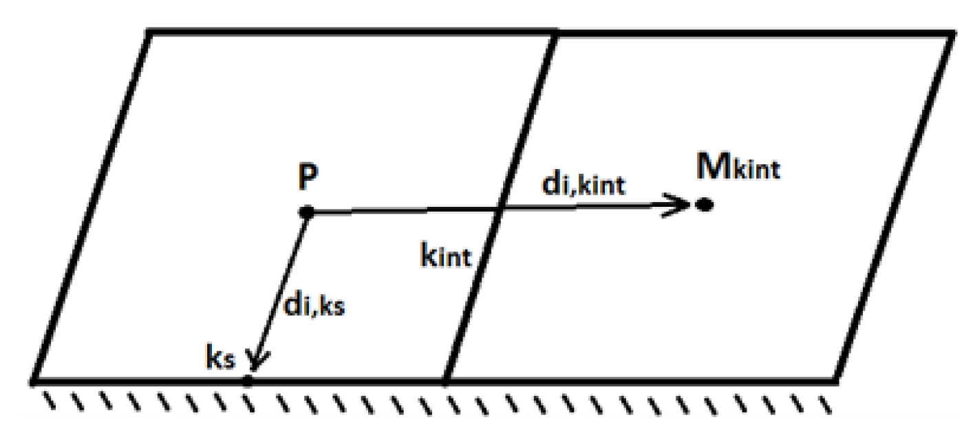
We consider an arbitrary unstructured grid, the view of which is shown in Figure 1:
Time discretization of Equation (3) according to the Adams–Beschfort scheme (the second-order scheme) is:
To discretize Equation (3) in space, we integrate it in terms of the volume of the cell “P” and proceed to area integration for the convective and diffusion terms:
The discrete analog of the diffusion term is written in the following form:
Here, is the normal of the face k. In the right part, under the sign of the sum in the product, there is a derivative in the direction , which, in the case of an orthogonal calculation, can be defined as follows:
For approximation on a finite-volume grid, the convective term is written as:
Here, is the volumetric flow through the face k. The value on the face of is determined by the applied sampling scheme of the convective term. There are a large number of sampling schemes that are applicable on arbitrary unstructured grids [62,63,64,65]. Among them, several schemes can be distinguished that have the “highest rating” of applicability in solving applied problems: counterflow scheme (Upwind Differences, UDs), counterflow scheme with linear interpolation (Linear Upwind Differences, LUDs), QUICK scheme, central difference scheme (Central Differences, CDs), schemes of the NVD family (Normalized Variable Diagram) and hybrid circuits (the above circuits mixed with a counterflow circuit to increase monotony).
Using this discretization, Equation (3) is replaced by a system of linear algebraic equations written for each calculation cell:
The resulting system of linear algebraic equations is solved using the AMG multigrid solver [56].
In an acoustic tomograph for the emission of acoustic waves, there are sources and a receiver that record the pressure. Sources and receivers are cylinders made of a material with acoustic parameters equal to water. The receiver records the entire pressure field inside the cylinder, and then the data of the inverse problem are averaged by volume.
To simulate an acoustic tomograph, the LOGOS software implements a technique that allows you to set the sources of acoustic waves, as well as process data in the receiver. The user can specify an arbitrary number of sources/receivers, specifying their location, size, the normal along which they are directed, and their status (that is, whether this “sensor” is a source or receiver). The source of acoustic waves is given as follows (Riker pulse):
where is the frequency. The acoustic wave source is included in the source , which is added to the momentum Equation (2), and looks like this:
Here, is the cell density, V is the cell volume, A is the amplitude, and is the normal in the direction of the signal. The pressure in each receiver is calculated by determining the cells that fall under the specified dimensions and location, and calculating the average pressure in the area of each receiver (volume integration).
3. Numerical Experiments
In this section, we consider a numerical simulation of the propagation of acoustic waves in the human body in order to study the possibility of determining liver pathologies with acoustic tomography.
Numerical calculations were performed for two cases: in the first case, two cubic inclusions are contained inside the mannequin symmetrically relative to the center—on the right, the inclusion parameters correspond to liver tissue, and on the left, adipose tissue; in the second case, two cubic inclusions are also located inside the mannequin, but the liver is surrounded by adipose tissue 0.5 cm thick. An acoustic tomograph is a cylinder filled with water. The parameters of the mannequin’s body correspond to the muscle tissue (see Table 1). Liver pathologies include many diseases, including neoplasms. We considered fatty liver disease, in which there is an excessive accumulation of fat in the liver. To simplify the situation, we assumed that the liver is covered with an additional layer of adipose tissue.
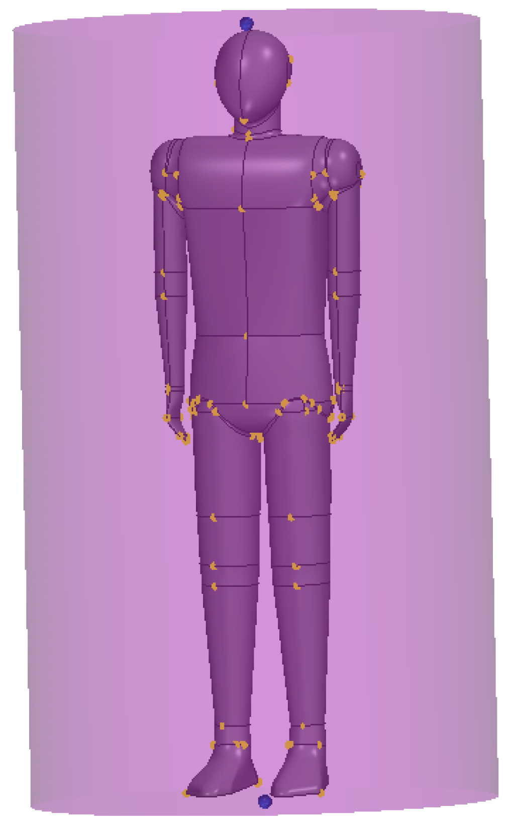
In Figure 2, we provide the scheme of the numerical experiment—the mannequin is located inside the tomograph (the cylinder):
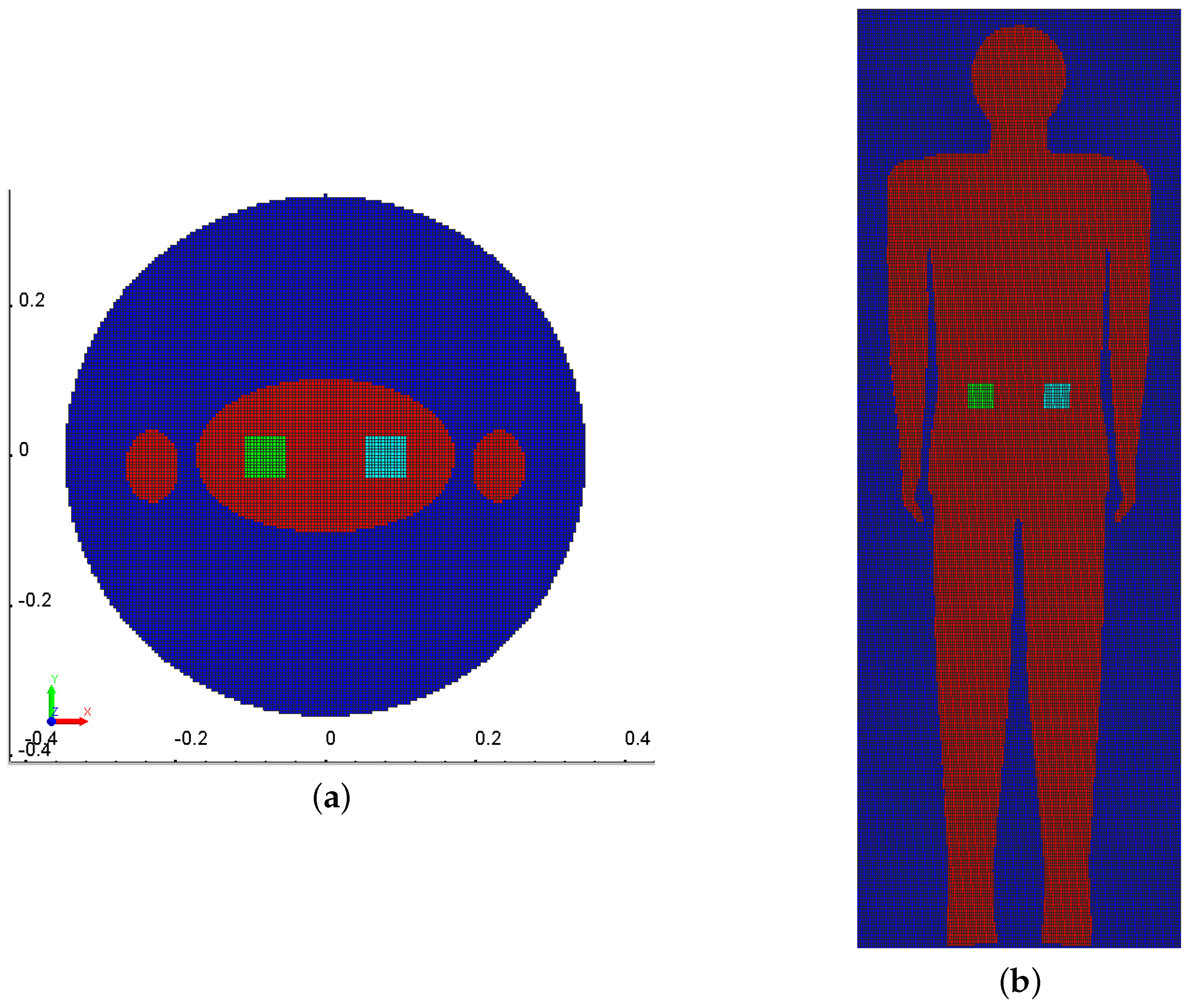
We use a block grid with a cell size of 0.004 m, consisting of 15 million cells, during the experiment. Figure 3 shows the resulting grid (in vertical and horizontal sections). At the initial moment of time, there are no disturbances, and the liquid in the tomograph is at rest.
The digital mannequin parameters are a height of 1.95 m, shoulder width of 0.56 m, and thickness of 0.34 m. Parameters of the tomograph (cylinder) are a height of 2 m and diameter of 0.7 m. Table 1 shows the acoustic parameters of the human body.
The mean parameters of the human body, presented in Table 1, were taken in accordance with [43,51,66,67].
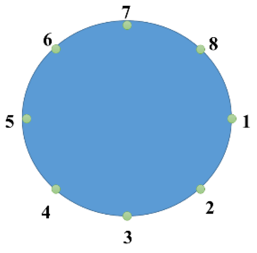
At the first stage, the calculation was carried out with two cubic inclusions, m, located symmetrically relative to the center inside the mannequin—liver (right) and adipose tissue (left). Eight transducers (sources and receivers) are located on the side of the tomograph at the level of the internal organs (Figure 4). The location of the source of the sounding wave in the calculations is marked with the number 3; all the others are receivers and record the pressure as a function of time. The source (receiver) is a cylinder with a diameter of 0.01 m and a height of 0.05 m made of a material with acoustic parameters equal to those of water. In the receiver, the pressure function captures the entire pressure field inside the cylinder and then averages by volume.
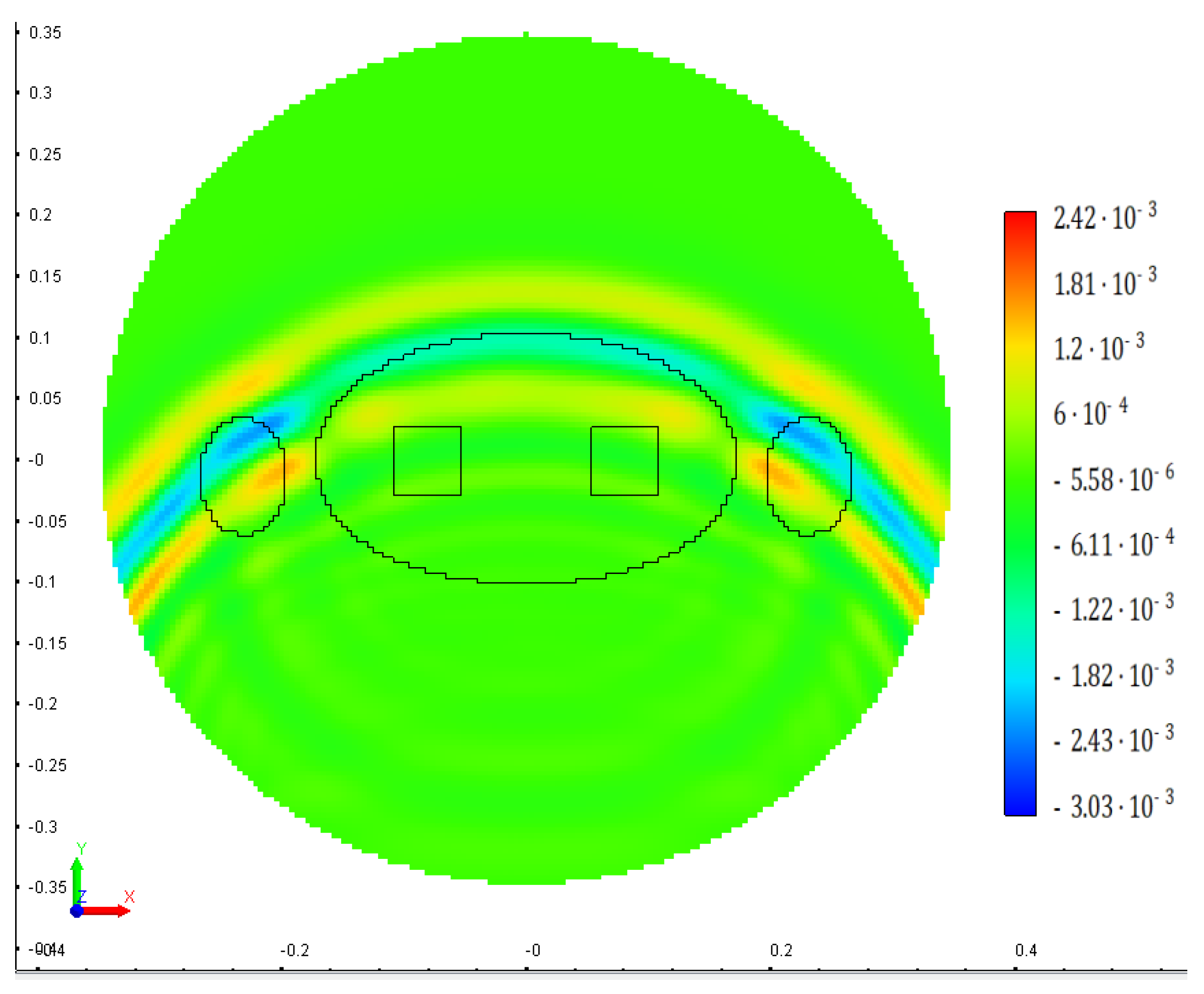
During the computations, we used the Ricker wavelet (4) with the frequency = 20,000 Hz. In Figure 5, we demonstrate the pressure field at s in a section located at a height in the center of the internal organs.
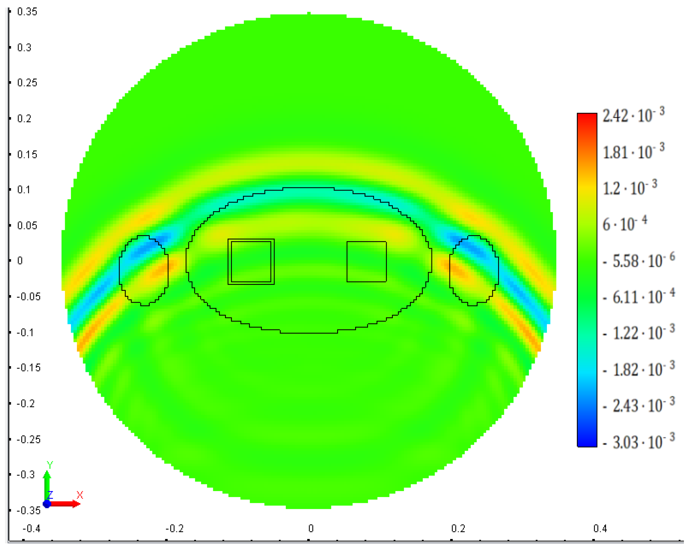
At the second stage, a calculation was carried out in which a cube with liver parameters is surrounded by a boundary layer with a thickness of cm. Thus, there are two cubic inclusions in the mannequin, located symmetrically relative to the center inside the mannequin: adipose tissue (left) with a size of m, and liver (right) with a size of m. Figure 6 shows the pressure field at time s in a cross section.
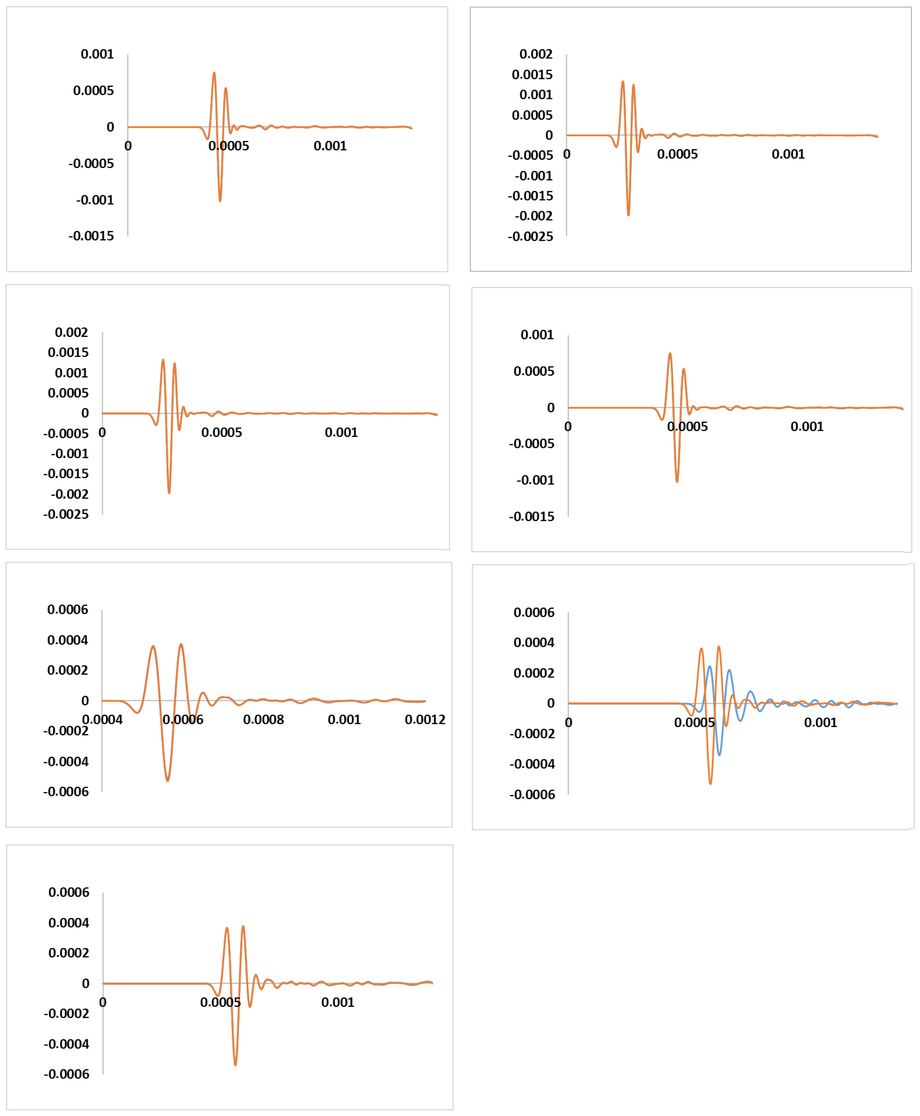
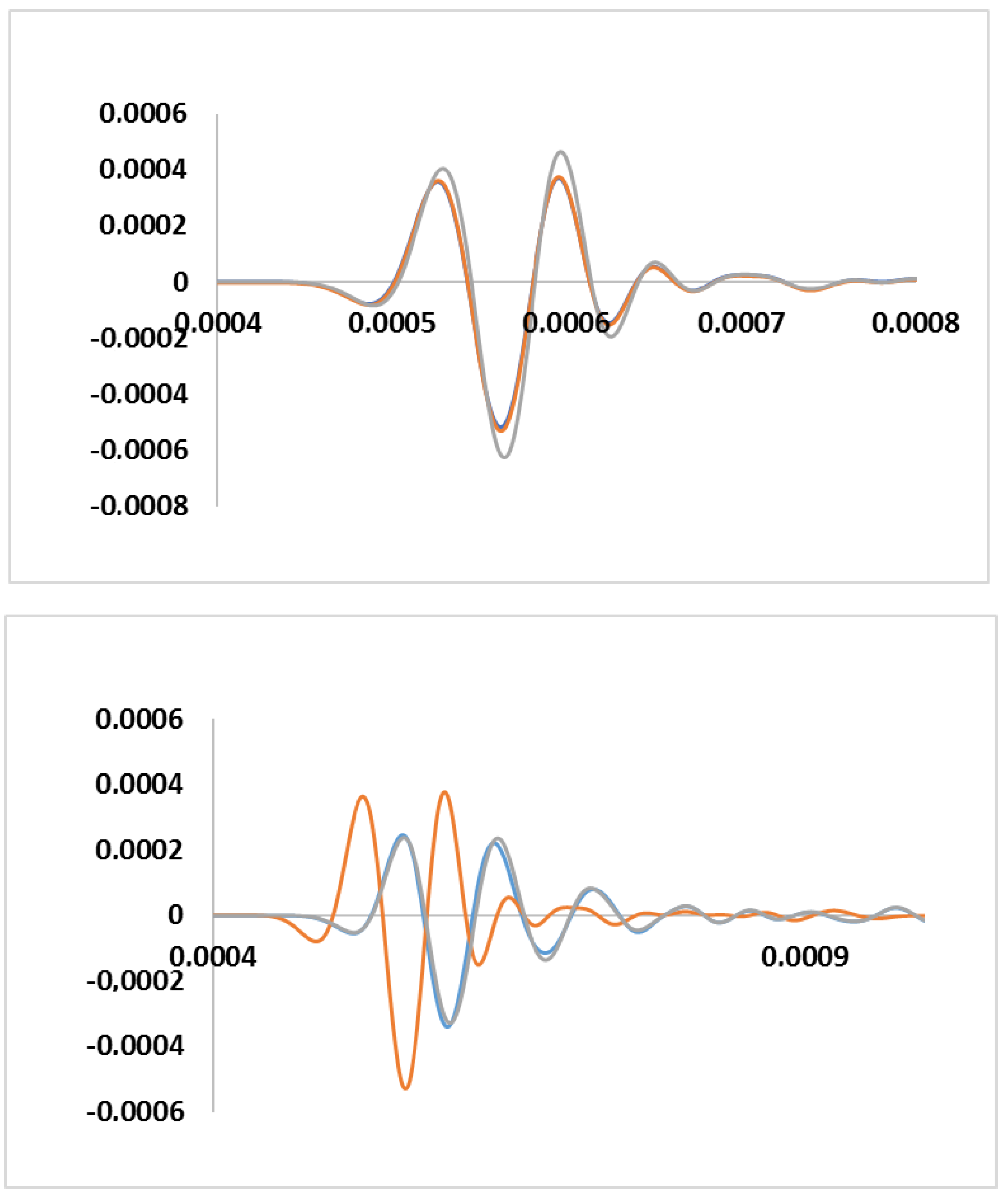
In Figure 7, one can see the pressure, registered in the receivers for both experiments.
Significant differences in pressure in the two calculations are observed in the 7th receiver. When the wave passes through the liver surrounded by adipose tissue, the pressure amplitude is increased compared to calculation 1, and the passage time of the acoustic waves is decreased due to the fact that the speed of sound in adipose tissue is higher than in water.
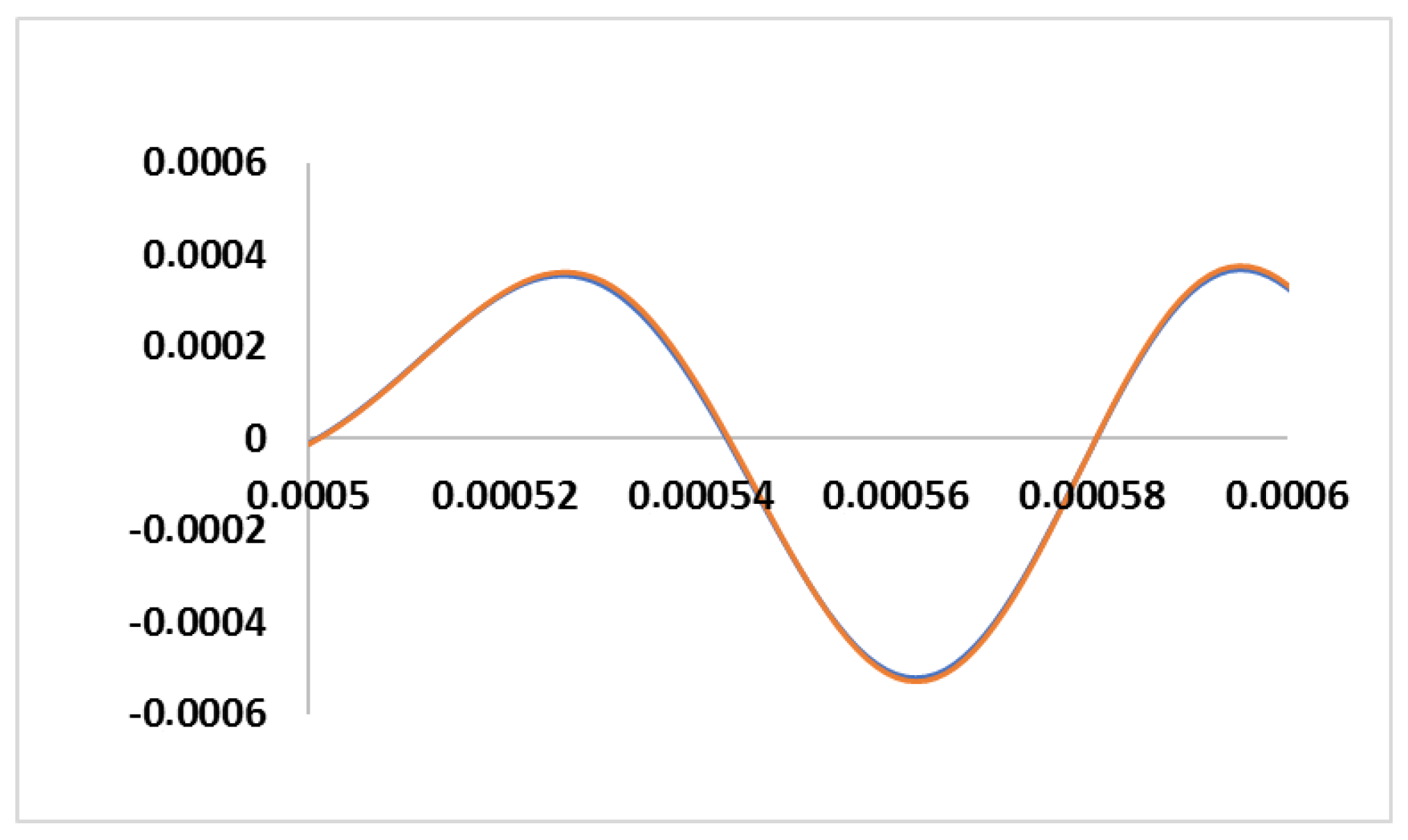
Minor differences are also observed in receiver 6 (Figure 8).
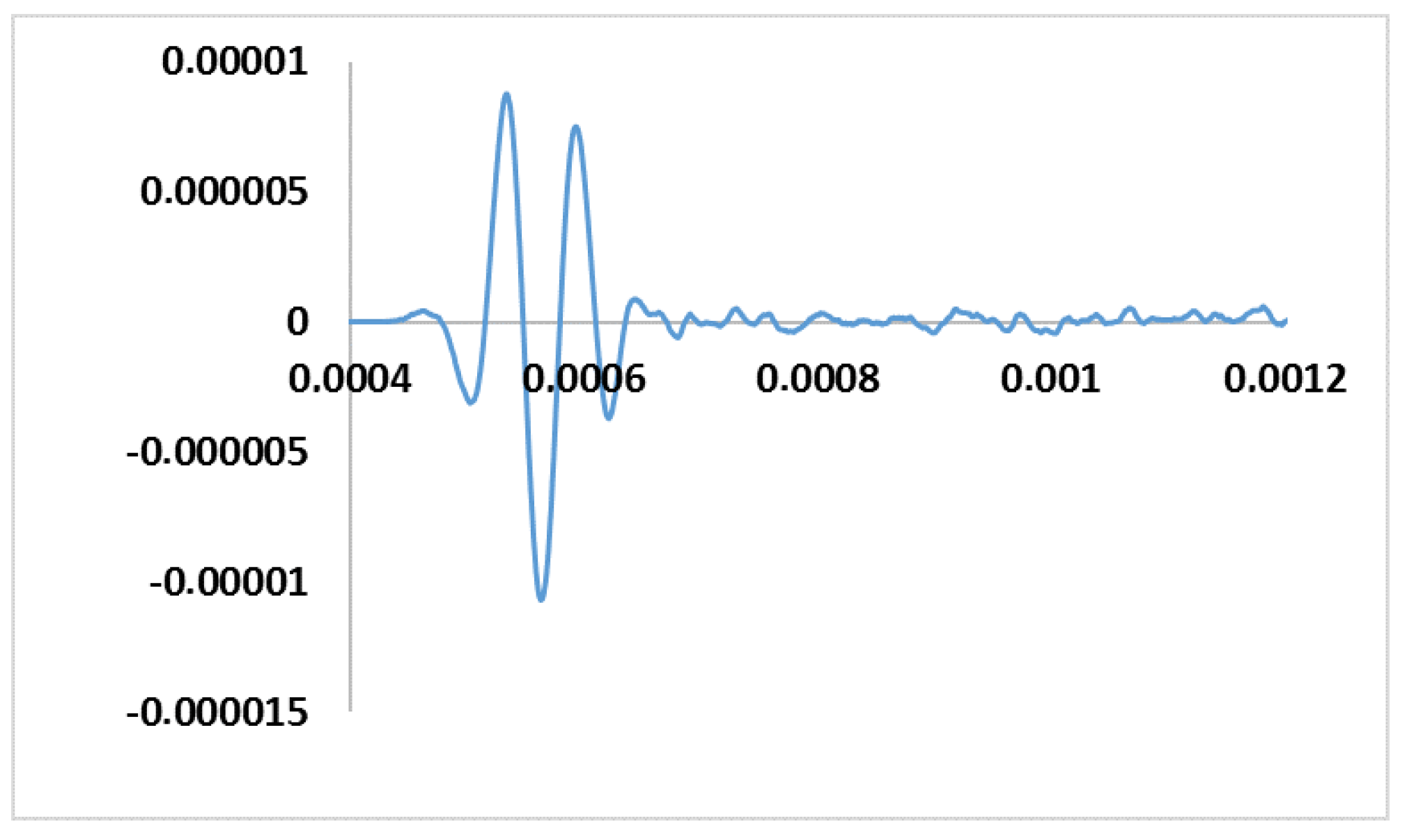
Figure 9 represents the quantitative difference of the registered pressure for the two experiments.
In order to test the efficiency of the technology, we carried out another numerical simulation, similar to calculation 2. The speed of sound in the adipose tissue surrounding the liver we set to 1000 m/s. Figure 10 shows graphs of pressure for three calculations in receivers 6 and 7, where the greatest difference is observed.
When a wave passes through the liver surrounded by adipose tissue at the speed of sound of 1000 m/s (experiment 3), the passage time of the acoustic waves to the receivers is increased compared to calculations 1 and 2. The pressure amplitude in receiver 6 is increased compared to experiments 1 and 2, and in receiver 7, it is lower compared to experiment 2.
4. Discussion
The article presents the results of the numerical simulation of acoustic wave propagation in the human body with nonlinear acoustic tomography based on the Navier–Stokes equations. This mathematical model takes into account most of the nonlinear effects of acoustic wave propagation, including shock waves. The computational technology presented in the article shows the fundamental possibility of using mathematical modeling methods based on the numerical solution of the complete hydrodynamic system of the Navier–Stokes equations to study the properties of acoustic waves during tomography of the human body. The introduction of such methods in the future will make it possible to understand almost all physical aspects of the functioning of such an ultrasound medical tomograph.
The article aimed to show the fundamental possibility of constructing a computational digital twin of the acoustic tomograph within the framework of a unified physics–mathematical model based on the Navier–Stokes equations. The authors proceeded from the fact that the size of the modeling area is quite small, sound waves are waves of “small” disturbance, and given that a human is more than 60% water, human organs can be modeled by a liquid model with their density. This is a kind of approximation in which, as in any model, there are assumptions, but it has the right to life and, in general, will allow us to determine the areas of change in the parameters of the sound wave to identify the required parameters. During numerical experiments, we obtained the pressure registered in the receivers that were located on the side walls of the tomograph. The differences in pressure values are shown depending on the configuration of inclusions in the mannequin imitating internal organs. The results show that the developed technology can be used to probe the human body in medical acoustic tomographs and determine the acoustic parameters of the human body to detect neoplasms. Numerical solution methods are currently being developed and implemented to solve inverse problems [68,69,70,71,72], as well as methods based on deep learning [73,74,75].
Author Contributions
Problem Formulation, M.S.; Methodology, A.K.; Software, A.K.; Validation, A.K.; Data curation, N.N.; Writing—original draft, A.K.; Writing—review & editing, M.S. and N.N.; Supervision, M.S.; Project administration, M.S.; Funding acquisition, M.S. All authors have read and agreed to the published version of the manuscript.
Funding
The work was supported by Russian Science Foundation, 19-11-00154 “Developing of new mathematical models of acoustic tomography in medicine. Numerical methods, HPC and software”.
Data Availability Statement
Data are contained within the article.
Conflicts of Interest
The authors declare no conflicts of interest.
References
- Strutt, J.W. The Theory of Sound; Cambridge University Press: Cambridge, UK, 2011; Volume 1. [Google Scholar]
- Strutt, J.W. The Theory of Sound; Cambridge University Press: Cambridge, UK, 2011; Volume 2. [Google Scholar]
- Li, S.; Jackowski, M.; Dione, D.P.; Varslot, T.; Staib, L.H.; Mueller, K. Refraction corrected transmission ultrasound computed tomography for application in breast imaging. Med. Phys. 2010, 37, 2233–2246. [Google Scholar] [CrossRef] [PubMed]
- Huthwaite, P.; Simonetti, F. High-resolution imaging without iteration: A fast and robust method for breast ultrasound tomography. J. Acoust. Soc. Am. 2011, 130, 1721–1734. [Google Scholar] [CrossRef] [PubMed]
- Duric, N.; Littrup, P.; Li, C.; Roy, O.; Schmidt, S.; Janer, R.; Cheng, X.; Goll, J.; Rama, O.; Bey-Knight, L.; et al. Breast ultrasound tomography: Bridging the gap to clinical practice. Proc. SPIE 2012, 8320, 832000. [Google Scholar]
- Jirik, R.; Peterlik, I.; Ruiter, N.; Fousek, J.; Dapp, R.; Zapf, M.; Jan, J. Sound-speed image reconstruction in sparse-aperture 3D ultrasound transmission tomography. IEEE Trans. Ultrason. Ferroelectr. Freq. Control 2012, 59, 254–264. [Google Scholar] [CrossRef] [PubMed]
- Marmot, M.G.; Altman, D.G.; Cameron, D.A.; Dewar, J.A.; Thompson, S.G.; Wilcox, M. The benefits and harms of breast cancer screening: An independent review. Br. J. Cancer 2013, 108, 2205–2240. [Google Scholar] [CrossRef] [PubMed]
- Birk, M.; Dapp, R.; Ruiter, N.V.; Becker, J. GPU-based iterative transmission reconstruction in 3D ultrasound computer tomography. J. Parallel Distrib. Comput. 2014, 74, 1730–1743. [Google Scholar] [CrossRef]
- Burov, V.A.; Zotov, D.I.; Rumyantseva, O.D. Reconstruction of the sound velocity and absorption spatial distributions in soft biological tissue phantoms from experimental ultrasound tomography data. Acoust. Phys. 2015, 61, 231–248. [Google Scholar] [CrossRef]
- Sandhu, G.Y.; Li, C.; Roy, O.; Schmidt, S.; Duric, N. Frequency domain ultrasound waveform tomography: Breast imaging using a ring transducer. Phys. Med. Biol. 2015, 60, 5381–5398. [Google Scholar] [CrossRef]
- Liu, H.; Uhlmann, G. Determining both sound speed and internal source in thermo- and photo-acoustic tomography. Inverse Probl. 2015, 31, 105005. [Google Scholar] [CrossRef]
- Huang, L.; Shin, J.; Chen, T.; Lin, Y.; Gao, K.; Intrator, M.; Hanson, K. Breast ultrasound tomography with two parallel transducer arrays. In Medical Imaging 2016: Physics of Medical Imaging (International Society for Optics and Photonics); SPIE: Bellingham, WA, USA, 2016; Volume 9783, p. 97830C. [Google Scholar]
- Matthews, T.P.; Wang, K.; Li, C.; Duric, N.; Anastasio, M.A. Regularized dual averaging image reconstruction for full-wave ultrasound computed tomography. IEEE Trans. Ultrason. Ferroelectr. Freq. Control 2017, 64, 811–825. [Google Scholar] [CrossRef]
- Opieliński, K.J.; Pruchnicki, P.; Szymanowski, P.; Szepieniec, W.K.; Szweda, H.; Świś, E.; Jóźwik, M.; Tenderenda, M.; Bułkowski, M. Multimodal ultrasound computer-assisted tomography: An approach to the recognition of breast lesions. Comput. Med. Imaging Graph. 2018, 65, 102–114. [Google Scholar] [CrossRef]
- Malik, B.; Terry, R.; Wiskin, J.; Lenox, M. Quantitative transmission ultrasound tomography: Imaging and performance characteristics. Med. Phys. 2018, 45, 3063–3075. [Google Scholar] [CrossRef] [PubMed]
- Guo, R.; Lu, G.; Qin, B.; Fei, B. Ultrasound imaging technologies for breast cancer detection and management: A review. Ultrasound Med. Biol. 2018, 44, 37–70. [Google Scholar] [CrossRef] [PubMed]
- Wiskin, J.; Malik, B.; Natesan, R.; Lenox, M. Quantitative assessment of breast density using transmission ultrasound tomography. Med. Phys. 2019, 46, 2610–2620. [Google Scholar] [CrossRef] [PubMed]
- Sood, R.; Rositch, A.F.; Shakoor, D.; Ambinder, E.; Pool, K.L.; Pollack, E.; Mollura, D.J.; Mullen, L.A.; Harvey, S.C. Ultrasound for breast cancer detection globally: A systematic review and meta-analysis. J. Glob. Oncol. 2019, 5, 1–17. [Google Scholar] [CrossRef] [PubMed]
- Vourtsis, A. Three-dimensional automated breast ultrasound: Technical aspects and first results. Diagn. Intervent. Radiol. 2019, 100, 579–592. [Google Scholar] [CrossRef]
- Park, C.K.S.; Xing, S.; Papernick, S.; Orlando, N.; Knull, E.; Toit, C.D.; Bax, J.S.; Gardi, L.; Barker, K.; Tessier, D.; et al. Spatially tracked whole-breast three-dimensional ultrasound system toward point-of-care breast cancer screening in high-risk women with dense breasts. Med. Phys. 2022, 49, 3944–3962. [Google Scholar] [CrossRef]
- Wang, K.; Matthews, T.; Anis, F.; Li, C.; Duric, N.; Anastasio, M.A. Waveform inversion with source encoding for breast sound speed reconstruction in ultrasound computed tomography. IEEE Trans. Ultrason. Ferroelectr. Freq. Control 2015, 62, 475–493. [Google Scholar] [CrossRef]
- Bernard, S.; Monteiller, V.; Komatitsch, D.; Lasaygues, P. Ultrasonic computed tomography based on full-waveform inversion for bone quantitative imaging. Phys. Med. Biol. 2017, 62, 7011–7035. [Google Scholar] [CrossRef]
- Pérez-Liva, M.; Herraiz, J.L.; Udías, J.M.; Miller, E.; Cox, B.T.; Treeby, B.E. Time domain reconstruction of sound speed and attenuation in ultrasound computed tomography using full wave inversion. J. Acoust. Soc. Am. 2017, 141, 1595–1604. [Google Scholar] [CrossRef]
- Filatova, V.; Danilin, A.; Nosikova, V.; Pestov, L. Supercomputer Simulations of the Medical Ultrasound Tomography Problem. Commun. Comput. Inf. Sci. 2019, 1063, 297–308. [Google Scholar]
- Kabanikhin, S.I.; Klyuchinskiy, D.V.; Novikov, N.S.; Shishlenin, M.A. Numerics of acoustical 2D tomography based on the conservation laws. J. Inverse Ill-Posed Probl. 2020, 28, 287–297. [Google Scholar] [CrossRef]
- Klyuchinskiy, D.; Novikov, N.; Shishlenin, M. Recovering density and speed of sound coefficients in the 2d hyperbolic system of acoustic equations of the first order by a finite number of observations. Mathematics 2021, 9, 199. [Google Scholar] [CrossRef]
- Filatova, V.; Pestov, L.; Poddubskaya, A. Detection of velocity and attenuation inclusions in the medical ultrasound tomography. J. Inverse Ill-Posed Probl. 2021, 29, 459–466. [Google Scholar] [CrossRef]
- Rumyantseva, O.D.; Shurup, A.S.; Zotov, D.I. Possibilities for separation of scalar and vector characteristics of acoustic scatterer in tomographic polychromatic regime. J. Inverse Ill-Posed Probl. 2021, 29, 407–420. [Google Scholar] [CrossRef]
- Shurup, A.S. Numerical comparison of iterative and functional-analytical algorithms for inverse acoustic scattering. Eurasian J. Math. Comput. Appl. 2022, 10, 79–99. [Google Scholar] [CrossRef]
- Lucka, F.; Pérez-Liva, M.; Treeby, B.E.; Cox, B.T. High resolution 3D ultrasonic breast imaging by time-domain full waveform inversion. Inverse Probl. 2022, 38, 025008. [Google Scholar] [CrossRef]
- Romanov, V.G.; Kabanikhin, S.I. Inverse Problems for Maxwell’s Equations; VSP: Utrecht, The Netherlands, 1994. [Google Scholar]
- Jafarzadeh, E.; Amini, M.H.; Sinclair, A.N. Spectral Shift Originating from Non-linear Ultrasonic Wave Propagation and Its Effect on Imaging Resolution. Ultrasound Med. Biol. 2021, 47, 1893–1903. [Google Scholar] [CrossRef]
- Campo-Valera, M.; Villó-Pérez, I.; Fernández-Garrido, A.; Rodríguez-Rodríguez, I.; Asorey-Cacheda, R. Exploring the Parametric Effect in Nonlinear Acoustic Waves. IEEE Access 2023, 11, 97221–97238. [Google Scholar] [CrossRef]
- Ichida, N.; Sato, T.; Linzer, M. Imaging the nonlinear ultrasonic parameter of a medium. Ultrason. Imaging 1983, 5, 295–299. [Google Scholar] [CrossRef]
- Lewin, P.A.; Nowicki, A. 16—Nonlinear acoustics and its application to biomedical ultrasonics. In Woodhead Publishing Series in Electronic and Optical Materials, Ultrasonic Transducers; Nakamura, K., Ed.; Woodhead Publishing: Cambridge, UK, 2012; pp. 517–544. [Google Scholar] [CrossRef]
- Meliani, M.; Nikolić, V. Analysis of General Shape Optimization Problems in Nonlinear Acoustics. Appl. Math. Optim. 2022, 86, 39. [Google Scholar] [CrossRef]
- Panfilova, A.; van Sloun, R.J.; Wijkstra, H.; Sapozhnikov, O.A.; Mischi, M. A review on B/A measurement methods with a clinical perspective. J. Acoust. Soc. Am. 2021, 149, 2200. [Google Scholar] [CrossRef]
- Tabak, G.; Oelze, M.L.; Singer, A.C. Effects of acoustic nonlinearity on communication performance in soft tissues. J. Acoust. Soc. Am. 2022, 152, 3583. [Google Scholar] [CrossRef]
- Kokumo, K.; Sharma, A.; Myers, K.; Ambinder, E.; Oluyemi, E.; Bell, M.A.L. Theoretical basis and experimental validation of harmonic coherence-based ultrasound imaging for breast mass diagnosis. In Medical Imaging 2023: Physics of Medical Imaging; SPIE: Bellingham, WA, USA, 2023; Volume 12463, pp. 95–104. [Google Scholar]
- Ferziger, J.H.; Peric, M. Computational Method for Fluid Dynamics; Springer: New York, NY, USA, 2002. [Google Scholar]
- Mozer, D.; Kim, J.; Mansour, N.N. DNS of Turbulent Channel Flow. J. Phys. Fluids 1999, 11, 943–945. [Google Scholar]
- Muir, T.G.; Carstensen, E.L. Prediction of nonlinear acoustic effects at biomedical frequencies and intensities. Ultrasound Med. Biol. 1980, 6, 345–357. [Google Scholar] [CrossRef] [PubMed]
- Okawai, H.; Kobayashi, K.; Nitta, S. An approach to acoustic properties of biological tissues using acoustic micrographs of attenuation constant and sound speed. J. Ultrasound Med. 2001, 20, 891–907. [Google Scholar] [CrossRef] [PubMed]
- Duck, F.A. Nonlinear acoustics in diagnostic ultrasound. Ultrasound Med. Biol. 2002, 28, 1–18. [Google Scholar] [CrossRef]
- Kaltenbacher, B. Mathematics of nonlinear acoustics. Evol. Equ. Control. Theory 2015, 4, 447–491. [Google Scholar] [CrossRef]
- Yu, T.; Cai, W. Simultaneous reconstruction of temperature and velocity fields using nonlinear acoustic tomography. Appl. Phys. Lett. 2019, 115, 104104. [Google Scholar] [CrossRef]
- Deng, Y.; Li, J.; Liu, H. On Identifying Magnetized Anomalies Using Geomagnetic Monitoring Within a Magnetohydrodynamic model. Arch. Ration. Mech. Anal. 2020, 235, 691–721. [Google Scholar] [CrossRef]
- Gan, W.S. Nonlinear Acoustical Imaging; Springer: Singapore, 2021. [Google Scholar]
- Kozelkov, A.S.; Krutyakova, O.G.L.; Kurulin, V.V.; Strelets, D.Y.E.; Shishlenin, M.A. The accuracy of numerical simulation of the acoustic wave propagations in a liquid medium based on Navier-Stokes equations. Sib. Electron. Math. Rep. 2021, 18, 1238–1250. [Google Scholar] [CrossRef]
- Maev, R.G.; Seviaryn, F. Applications of non-linear acoustics for quality control and material characterization. J. Appl. Phys. 2022, 132, 161101. [Google Scholar] [CrossRef]
- Chen, P.; Pollet, A.M.; Panfilova, A.; Zhou, M.; Turco, S.; den Toonder, J.M.; Mischi, M. Acoustic characterization of tissue-mimicking materials for ultrasound perfusion imaging research. Ultrasound Med. Biol. 2022, 48, 124–142. [Google Scholar] [CrossRef]
- Gemmeke, H.; Hopp, T.; Zapf, M.; Kaiser, C.; Ruiter, N.V. 3D ultrasound computer tomography: Hardware setup, reconstruction methods and first clinical results. Nucl. Instrum. Methods Phys. Res. Sect. A Accel. Spectrometers Detect. Assoc. Equip. 2017, 873, 59–65. [Google Scholar] [CrossRef]
- Zhang, Y. Nonlinear acoustic imaging with damping. arXiv 2023, arXiv:2302.14174. [Google Scholar]
- Wiskin, J.; Malik, B.; Klock, J. Low frequency 3D transmission ultrasound tomography: Technical details and clinical implications. Z. Med. Phys. 2023, 33, 427–443. [Google Scholar] [CrossRef]
- Wiskin, J.; Malik, B.; Ruoff, C.; Pirshafiey, N.; Lenox, M.; Klock, J. Whole-Body Imaging Using Low Frequency Transmission Ultrasound. Acad. Radiol. 2023, 30, 2674–2685. [Google Scholar] [CrossRef]
- Lashkin, S.V.; Kozelkov, A.S.; Yalozo, A.V.; Gerasimov, V.Y.; Zelensky, D.K. Efficiency analysis of the parallel implementation of the simple algorithm on multiprocessor computers. J. Appl. Mech. Tech. Phys. 2017, 58, 1242–1259. [Google Scholar] [CrossRef]
- Kozelkov, A.; Tyatyushkina, E.; Kurkin, A.; Kurulin, V.; Kurkina, O.; Kochetkova, O. Fluid flow simulation in a T-connection of square pipes using modern approaches to turbulence modeling. Sib. Electron. Math. Rep. 2023, 20, 25–46. [Google Scholar]
- Kozelkov, A.; Kurkin, A.; Utkin, D.; Tyatyushkina, E.; Kurulin, V.; Strelets, D. Application of Non-Reflective Boundary Conditions in Three-Dimensional Numerical Simulations of Free-Surface Flow Problems. Geosciences 2022, 12, 427. [Google Scholar] [CrossRef]
- Kozelkov, A.S.; Lashkin, S.V.; Efremov, V.R.; Volkov, K.N.; Tsibereva, Y.A.; Tarasova, N.V. An implicit algorithm of solving Navier–Stokes equations to simulate flows in anisotropic porous media. Comput. Fluids 2018, 160, 164–174. [Google Scholar] [CrossRef]
- Chen, Z.J.; Przekwas, A.J. A coupled pressure-based computational method for incompressible/compressible flows. J. Comput. Phys. 2010, 229, 9150–9165. [Google Scholar] [CrossRef]
- Moukalled, F.; Darwish, M. Pressure-Based Algorithms for Multi-Fluid Flow at All Speeds—Part I: Mass Conservation Formulation, Numerical Heat Transfer. Part B Fundam. 2004, 45, 495–522. [Google Scholar] [CrossRef]
- Jasak, H. Error Analysis and Estimation for the Finite Volume Method with Applications to Fluid Flows. Ph.D. Thesis, Department of Mechanical Engineering, Imperial College of Science, London, UK, 1996. [Google Scholar]
- Jasak, H.; Weller, H.G.; Gosman, A.D. High resolution NVD differencing scheme for arbitrarily unstructured meshes. Int. J. Numer. Methods Fluids 1999, 31, 431–449. [Google Scholar] [CrossRef]
- Leonard, B.P. A stable and accurate convective modeling procedure based on quadratic upstream interpolation. Comput. Methods Appl. Mech./Eng. 1979, 19, 59–98. [Google Scholar] [CrossRef]
- Gaskell, P.H. Curvature-compensated convective-transport—SMART, A new boundedness-preserving transport algorithm. Int. J. Numer. Methods Fluids 1988, 8, 617–641. [Google Scholar] [CrossRef]
- Goss, S.A.; Johnston, R.L.; Dunn, F. Comprehensive compilation of empirical ultrasonic properties of mammalian tissues. J. Acoust. Soc. Am. 1978, 64, 423–457. [Google Scholar] [CrossRef]
- Mast, T.D. Empirical relationships between acoustic parameters in human soft tissues. Acoust. Res. Lett. 2000, 1, 37–42. [Google Scholar] [CrossRef]
- Klyuchinskiy, D.; Novikov, N.; Shishlenin, M. A Modification of gradient descent method for solving coefficient inverse problem for acoustics equations. Computation 2020, 8, 73. [Google Scholar] [CrossRef]
- Shishlenin, M.A.; Savchenko, N.A.; Novikov, N.S.; Klyuchinskiy, D.V. On the reconstruction of the absorption coefficient for the 2D acoustic system. Sib. Electron. Math. Rep. 2023, 20, 1474–1489. [Google Scholar]
- Klyuchinskiy, D.V.; Novikov, N.S.; Shishlenin, M.A. CPU-time and RAM memory optimization for solving dynamic inverse problems using gradient-based approach. J. Comput. Phys. 2021, 439, 110374. [Google Scholar] [CrossRef]
- Jenaliyev, M.T.; Bektemesov, M.A.; Yergaliyev, M.G. On an inverse problem for a linearized system of Navier–Stokes equations with a final overdetermination condition. J. Inverse Ill-Posed Probl. 2023, 31, 611–624. [Google Scholar] [CrossRef]
- Wang, Z.; Dulikravich, G. A numerical Method for Solving Cascade Inverse Problems Using Navier-Stokes Equations. 33rd Aerospace Sciences Meeting and Exhibit. 1995. Published Online: 22 August 2012. Available online: https://arc.aiaa.org/doi/abs/10.2514/6.1995-304 (accessed on 20 November 2023).
- Arridge, S.; Maass, P.; Öktem, O.; Schönlieb, C. Solving inverse problems using data-driven models. Acta Numer. 2019, 28, 1–174. [Google Scholar] [CrossRef]
- Basurto-Hurtado, J.A.; Cruz-Albarran, I.A.; Toledano-Ayala, M.; Ibarra-Manzano, M.A.; Morales-Hernandez, L.A.; Perez-Ramirez, C.A. Diagnostic Strategies for Breast Cancer Detection: From Image Generation to Classification Strategies Using Artificial Intelligence Algorithms. Cancers 2022, 14, 3442. [Google Scholar] [CrossRef]
- Fan, Y.; Wang, H.; Gemmeke, H.; Hopp, T.; Hesser, J. Model-data-driven image reconstruction with neural networks for ultrasound computed tomography breast imaging. Neurocomputing 2022, 467, 10–21. [Google Scholar] [CrossRef]
Figure 1.
The calculated grid k is the set of faces of the cell “P”, which is composed of a set of inner faces of and a set of outer faces of . The neighboring cell along the inner face of is denoted by . The vector is the area of the face k—, where is the number of the vector component. The vector from the center of cell “P” to the center of cell “M” along the face is denoted as , and the vector from the center of “P” to the center of the face is , where is the radius vector.

Figure 2.
The digital mannequin of the human body inside the acoustic tomograph.

Figure 3.
Constructed block grid: (a) calculated grid in the horizontal section, (b) calculated grid in the vertical section.
Figure 3.
Constructed block grid: (a) calculated grid in the horizontal section, (b) calculated grid in the vertical section.

Figure 4.
The location of sources and receivers.

Figure 5.
Experiment 1—the pressure field at s.

Figure 6.
Experiment 2—the pressure field at s.

Figure 7.
Comparison of two calculations (calculation 1—there is no layer of adipose tissue around the liver; calculation 2—the liver is surrounded by a layer of adipose tissue 0.01 m thick).
Figure 7.
Comparison of two calculations (calculation 1—there is no layer of adipose tissue around the liver; calculation 2—the liver is surrounded by a layer of adipose tissue 0.01 m thick).

Figure 8.
Comparison of pressure in receiver 6.

Figure 9.
The registered pressure for the two experiments.

Figure 10.
Comparison of two calculations (experiment 1—there is no layer of adipose tissue around the liver; experiment 2—the liver is surrounded by a layer of adipose tissue at a sound speed of 1460 m/s; experiment 3—the liver is surrounded by a layer of adipose tissue at a sound speed of 1000 m/s.


Table 1.
Acoustic parameters of the human body.
| Speed of Sound, m/s | Density, kg/m3 | |
|---|---|---|
| Muscular tissue | 1550 | 994 |
| Adipose tissue | 1460 | 904 |
| Liver | 1570 | 1083 |
Disclaimer/Publisher’s Note: The statements, opinions and data contained in all publications are solely those of the individual author(s) and contributor(s) and not of MDPI and/or the editor(s). MDPI and/or the editor(s) disclaim responsibility for any injury to people or property resulting from any ideas, methods, instructions or products referred to in the content. |
© 2024 by the authors. Licensee MDPI, Basel, Switzerland. This article is an open access article distributed under the terms and conditions of the Creative Commons Attribution (CC BY) license (https://creativecommons.org/licenses/by/4.0/).
Share and Cite
MDPI and ACS Style
Shishlenin, M.; Kozelkov, A.; Novikov, N. Nonlinear Medical Ultrasound Tomography: 3D Modeling of Sound Wave Propagation in Human Tissues. Mathematics 2024, 12, 212. https://doi.org/10.3390/math12020212
AMA Style
Shishlenin M, Kozelkov A, Novikov N. Nonlinear Medical Ultrasound Tomography: 3D Modeling of Sound Wave Propagation in Human Tissues. Mathematics. 2024; 12(2):212. https://doi.org/10.3390/math12020212
Chicago/Turabian StyleShishlenin, Maxim, Andrey Kozelkov, and Nikita Novikov. 2024. "Nonlinear Medical Ultrasound Tomography: 3D Modeling of Sound Wave Propagation in Human Tissues" Mathematics 12, no. 2: 212. https://doi.org/10.3390/math12020212
Note that from the first issue of 2016, this journal uses article numbers instead of page numbers. See further details here.