Computer Model for an Intelligent Adjustment of Weather Conditions Based on Spatial Features for Soil Moisture Estimation

Abstract

In this paper, an intelligent weather conditions fuzzy adjustment based on spatial features (IWeCASF) is developed. It is indispensable for our regional soil moisture estimation approach, complementing a point estimation model of soil moisture from the literature. The point estimation model requires the weather conditions at the point where an estimate is made. Therefore, IWeCASF’s aim is to determine these weather conditions. The procedure begins measuring them at only one checkpoint, called the primary checkpoint. The model determines the weather conditions anywhere within a region through image processing algorithms and fuzzy inference systems. The results are compared with the measurement records and with a spatial interpolation method. The performance is similar to or better than interpolation, especially in the rain, where the model developed is more accurate due to the certainty of replication. Additionally, IWeCASF does not require more than one measurement point. Therefore, it is a more appropriate approach to complement the point estimation model for enabling a regional soil moisture estimation.

1. Introduction

Automatic irrigation systems decrease water consumption [1,2]. In these systems, soil moisture is generally obtained using interconnected measuring instruments to determine the water supply. Some works have developed low-cost sensor networks to monitor agronomic and environmental variables; for example, in [3]. Nonetheless, the implementation complexity and maintenance of a measuring sensor network increase the cost of automatic irrigation systems, which can be an issue, especially in small farms [4,5]. An alternative for reducing the physical complexity of measuring networks is estimating soil moisture instead of measuring in situ [6,7]. In many applications, combining measurements and estimates is frequent [8,9,10]. In this sense, hybrid systems (measurements and estimations) can be an alternative for reducing the physical complexity of measurement networks to estimate soil moisture instead of measuring it in all relevant points.

Some soil moisture estimation developments are hydrological models [11,12,13,14,15]. Likewise, soil water balance calculations [16,17,18], remote sensing using microwaves [19], artificial neural networks (ANNs) [20,21,22,23,24,25,26], and supported vector machines (SVMs) [27,28,29,30] have several advantages. All these models present an accurate estimate of soil moisture but have limitations for implementation in small farms. The input data acquisition for hydrological models is complicated, as are the assumptions made to develop the model. Soil water balance calculations require regular recalibration. In remote sensing, microwave sensors’ implementation on satellites and the resolution scale (~25 to 50 km) are the problem. ANN and SVM training stages require many tests and a large sample data set to estimate soil moisture accurately.

Remote sensing techniques (RSs) have several advantages for evaluating soil properties and moisture, including large-scale coverage, a non-destructive nature, monitoring, multispectral capabilities, and rapid data acquisition. The specific context and objective of the soil measurements can determine the most suitable RS technique [31]. Other works address the potential of utilizing remotely sensed vegetation and soil moisture observations; likewise, they integrate remote sensing data sets to constrain the uncertainty of irrigation modeling [32]. Several RS options are available to the agricultural community. However, the farm sector has yet to fully implement RS technologies due to knowledge gaps in their sufficiency, appropriateness, and techno-economic feasibility [33]. However, RS assists the adaptive evolution of farm practices to face this significant challenge by providing periodic information on crops throughout the season at distinct scales [34].

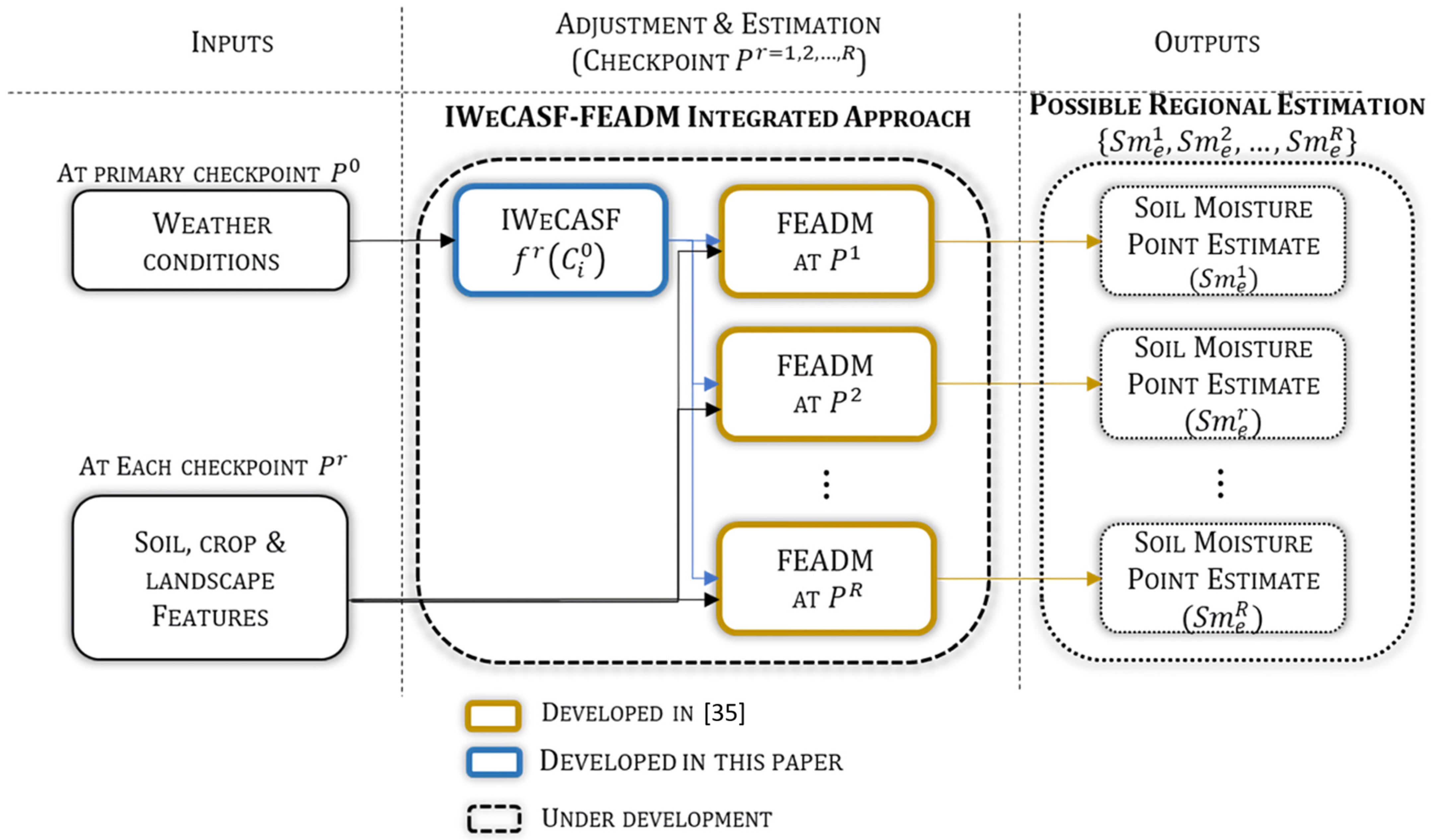
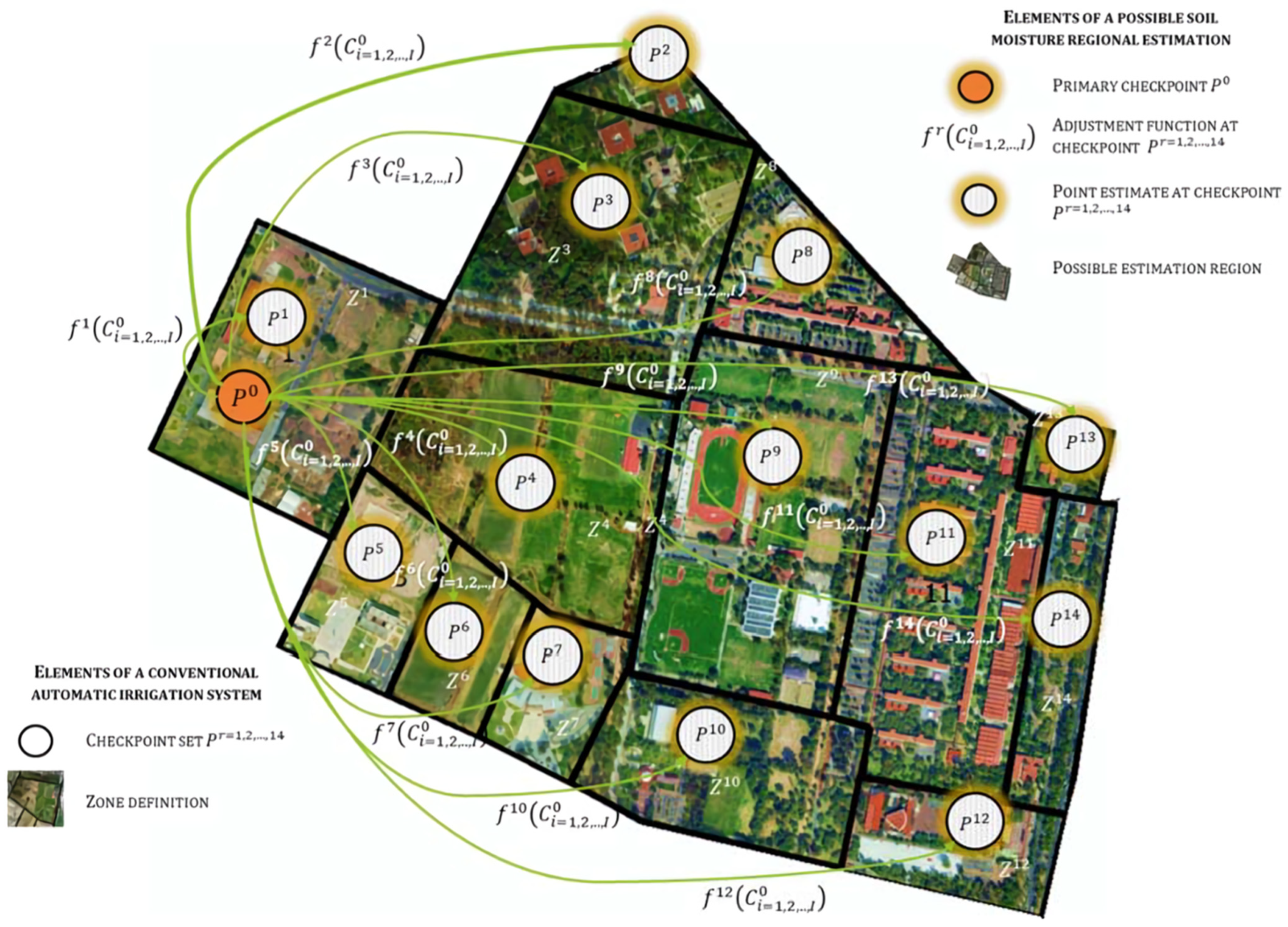
Another estimation approach to soil moisture is the fuzzy estimation approach based on decision making (FEADM) developed in [35] and called the point estimation model in this paper. The estimate is derived from modeling the interactions among soil moisture, weather conditions, crop, and soil. As shown in [35], the point estimation model uses a small number of measurement sensors and reduces the necessary calibration tests. However, the point estimation model estimates soil moisture only at one checkpoint (point estimate); if a regional estimation (set of point estimates) is pretended, this model needs to be executed at each checkpoint of the region. The point estimation model alone is not appropriate for a regional estimation because it requires the weather conditions where a point estimate is made. Measuring weather conditions at each checkpoint could be more complicated than deploying a network of soil moisture measuring sensors.

This paper aims to develop a computer model that helps the point estimation model avoid the issues related to the acquisition of weather conditions, as mentioned above. The model developed herein is the intelligent weather conditions adjustment based on spatial features (IWeCASF), called the adjustment model throughout this paper. The adjustment model is not a soil moisture estimation approach but can be part of a regional estimation model described in Section 2.

Some weather conditions can be considered similar within a region [22]. Fuzzy logic models for soil moisture content have been used for estimation, and they can contribute to diverse engineering applications such as plantation, crops production, and irrigation [36]. However, variations are caused by landscape features, the year’s season, and interactions among weather conditions. The adjustment model adapts the weather conditions measured at a primary checkpoint, considering the various factors that affect weather conditions at the other checkpoints. The purpose of the adjustment model (IWeCASF) is to determine the weather conditions at every region’s checkpoint.

The adjustment model performs an automatic and portable extraction of the landscape features from satellite imagery. Then, fuzzy adjustments of weather conditions are conducted based on the interactions of landscape features, checkpoint location, and weather conditions measured at the primary checkpoint. Also, a certainty index of weather condition replication is introduced to contemplate the year’s season’s effects. The result is an adjustment factor for each checkpoint derived from the steady elements (landscape features) and variable elements (season of the year and weather conditions interactions).

This paper is presented in six sections. Section 2 describes the importance of the adjustment model in a regional estimation based on the point estimation model [35], which was developed for our research team. In Section 3, the adjustment model is developed. Section 4 presents the results and discussion of the weather condition adjustment under several tests. Finally, Section 5 contains the conclusions.

2. The Adjustment Model as Part of a Regional Estimation Based on Point Estimates

A regional estimation based on the point estimation model can be achieved when a point estimate is made at every region’s checkpoint. In this way, the issues of a sensor network derived from measuring soil moisture at all points can be discarded. As mentioned in the previous section, the point estimation model alone is not appropriate for performing a regional estimation; it requires a complementary model.

Figure 1 depicts an illustrative irrigation region, a checkpoint set, and the regional estimation. A point estimate is intended at each checkpoint of the set. The regional estimation operation based on the point estimation model (FEADM) [35] is the following: first, weather conditions $C_i^0$ (inputs) are measured at the primary checkpoint ($P^0)$. Then, an adjustment model ($f^R\left(C_i^0\right)$) determines weather conditions at every checkpoint ($P^{r=\mathrm{1,2},\dots ,14}$). Finally, the point estimation model uses the weather conditions from the adjustment model ($f^R\left(C_i^0\right)$) and the land features of the checkpoint to perform a point estimate of soil moisture. The set of point estimates would be the regional estimate. This regional estimation is based on the interactions of soil moisture and environmental conditions (landscape features and weather conditions); consequently, it is intended to be used only in open-sky agriculture.

The adjustment model $f^R\left(C_i^0\right)$ can be developed using some methods from the literature, such as inverse distance weighting (IDW) [37,38], kriging, and co-kriging [39,40]. These spatial interpolation methods are widely used to estimate weather conditions in large areas. However, they show limitations when utilized in a regional estimation as proposed in this section because spatial interpolation models use a network of measurement points: rainfall is not remarkably homogenous in a region; thus, basing its interpolation value only on spatial measurements or statistical records can be misleading.

Unlike spatial interpolation methods, the adjustment model developed herein does not require deploying a sensor network and considers rainfall inconsistencies. Therefore, in a regional estimation, as proposed, this model is more suitable for utilization as the adjustment function $f^R\left(C_i^0\right)$ (adjustment model). The regional estimation scheme based on the point estimation and the adjustment model is presented in Figure 2. In this paper, no soil moisture estimate is made: a point estimate is already given and probed in [35]; the regional estimation, as well as factors such as problems derived from overirrigation, salinity water, or animal habitats, is not presented due to extension constraints. Only the adjustment model (weather conditions adjusted) is developed and tested in this paper.

3. Materials and Methods

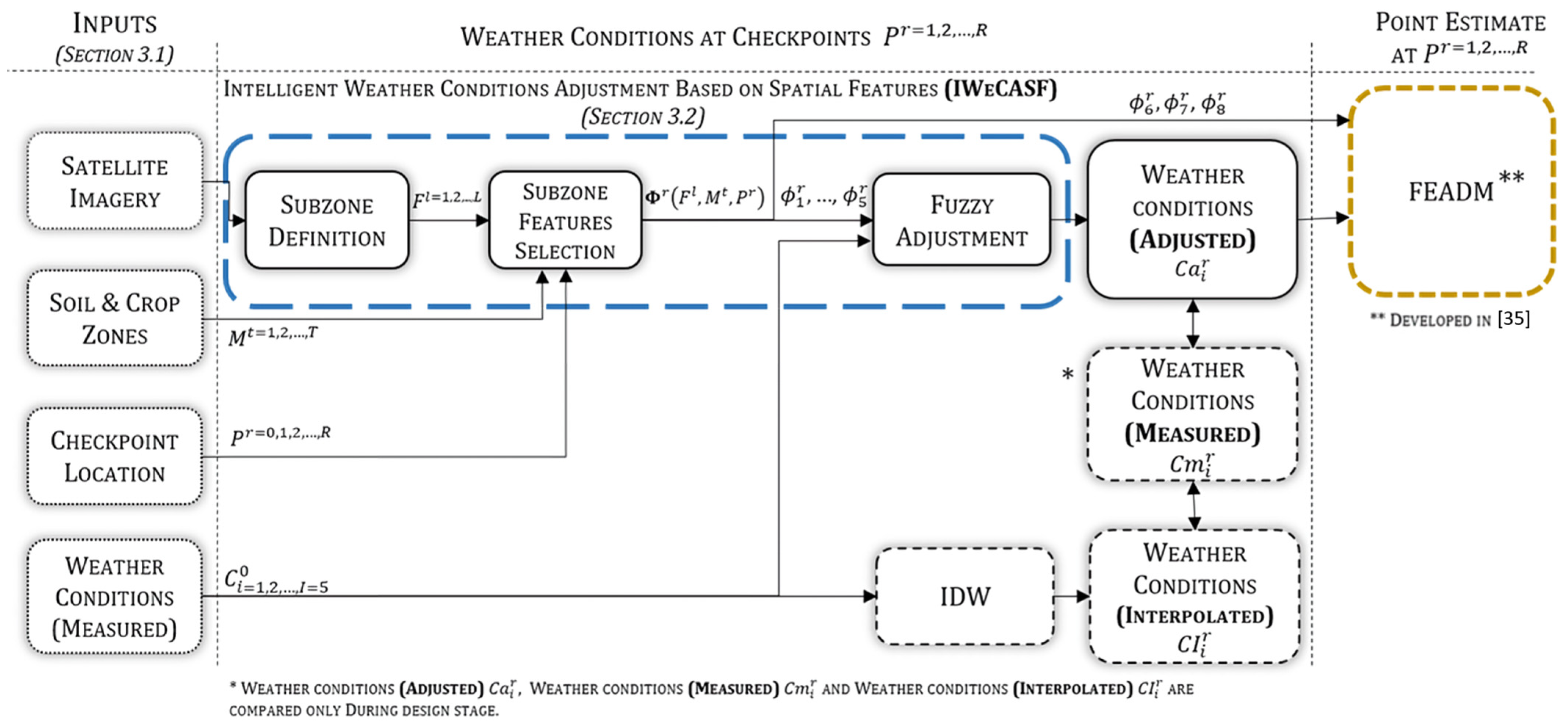
The adjustment model performs three main automatic tasks: landscape feature extraction, selection of particular landscape features, and adjustment of the weather conditions at every region’s checkpoint.

Figure 3 presents the adjustment model overview. The inputs processed are geographic data such as satellite imagery, soil and crop features ($M^{t=\mathrm{1,2},\dots ,T}$), checkpoint location ($P^{r=\mathrm{0,1},\dots ,R})$, and measurements of the weather conditions ($C_{i=\mathrm{1,2},\dots ,I}^0$). Then, landscape matrices ($F^{l=\mathrm{1,2},\dots ,L}$) are extracted from the satellite imagery in the subzone definition.

Afterwards, particular features (${\mathsf{\Phi }}^r(F^l,M^t,P^r)$), i.e., the checkpoint’s features (grasslands, tree-covered areas, buildings areas, elevation, spatial configuration, soil type, crop type, and crop stage), are selected in subzone features selection. Particular features are utilized in the fuzzy adjustment to achieve the weather conditions adjusted (${Ca}_i^r)$. A set of integrated sensor suite was installed at several checkpoints to compare the weather conditions adjusted (${Ca}_i^r)$ with weather conditions measured ${Cm}_i^r$ and weather conditions interpolated (${CI}_i^r)$ derived from IDW, a model from the literature. This comparison is performed only during the design stage to validate the results, and it is not necessary for the adjustment model operation.

3.1. Inputs

3.1.1. Satellite Imagery

The satellite imagery was acquired using the USGS National Map Viewer, downloaded from Landsat in March 2017. It is processed using the QGIS [41]. The scale is 1:10,000. The region used to develop the adjustment model corresponds to a basin that stretches for almost 2 km. There are buildings, roads, grassy areas, and tree-covered areas. The landscape characteristics of this region are more complex than those of purely agricultural lands. A more complex region such as the one utilized allows for testing the adjustment model with different landscape features under controlled conditions.

Each satellite image is divided into $S$ sectors, giving a result of pairwise sectors ($s\left(x,y\right)$), where $x=\mathrm{1,2},\dots ,X, \mathrm{y}=\mathrm{1,2},\dots ,Y$, $X$ is the image width divided into $S$ sectors, and $Y$ is the image height divided into $S$ sectors. A sector $s(x,y)$ is a small area of the region; its size is defined by the maximum extent to which, in all sectors, one landscape feature prevails. Preliminary tests were conducted to obtain an appropriate size and resolution of the image; these tests avoid uncertainties in the feature selection stage and error propagation. For instance, the satellite image of the region is shown in Figure 4. The size of each sector is $40\times 40 \mathrm{m}$; the image is divided into S = 2150 sectors. The image resolution is 145$0\times 1247$ pixels, i.e., one pixel represents approximately 1.8${\mathrm{m}}^2$.

3.1.2. Soil and Crop Features

The soil and crop features are geographic data (soil type, crop type, and crop stage). Soil and crop features are not entirely related to the weather conditions adjustment; however, the adjustment model processes them to the point estimation model in which soil and crop features are wholly utilized. Soil and crop features are defined and classified according to the point estimation model [35]. Other soil parameters involved in soil moisture estimation, such as the vertical distribution of water and the root depths, are not considered in soil and crop features because these parameters are determined internally in the point estimation model.

Two databases compound soil and crop features. The first contains geo-information of the region divided into zones according to field capacity and available water content. These properties define the soil type because they are highly interrelated, e.g., when soil moisture exceeds field capacity, it drains through lower soil levels due to reduced available water content [42].

Table 1. Soil texture, field capacity, and available water content.

Type	$\mathbf{Field} \mathbf{Capacity} (\mathbf{FC}) \left({\mathbf{m}}^3/{\mathbf{m}}^3\right)$	$\mathbf{Available} \mathbf{Water} \mathbf{Content} (\mathbf{AWC}) \left({\mathbf{m}}^3/{\mathbf{m}}^3\right)$
$\mathrm{I}$	$FC\le 0.21$	$AWC\le 0.08$
$\mathrm{I}\mathrm{I}$	$0.21<FC\le$ 0.44	$0.08<AWC\le 0.21$
$\mathrm{I}\mathrm{I}\mathrm{I}$	$0.44<FC$	$0.21<AWC$

shows the soil type classification.

The second database is geo-information of crop properties such as crop type or development stage. Depending on crop type and stage, the crop can withstand different soil moisture levels [43]. Specific crops, such as rice, require a high water supply; meanwhile, other crops such as beans can grow under a lower water supply. In addition, the crop can be more sensitive to water during flowering or grain-filling stages. The crop types and stages are defined according to the Food and Agriculture Organization (FAO) Indicative Crop Classification (ICC) of the agricultural consensus [44].

Both geographic databases are used to develop the feature matrices $M^{t=\mathrm{1,2},\dots ,T}$, where $T$ is the total of features (soil type, crop type, and crop stage). The feature matrices $M^{t=\mathrm{1,2},\dots ,T}$ are the following:

• $M^{t=1}$ contains soil type data.
• $M^{t=2}$ contains crop type data.
• $M^{t=3}$ contains crop stage data.

Feature matrices are the same size ($X\times Y$) as satellite image matrices. Each element $m_{x,y}^t$ of the feature matrices represents the feature $t$ at the sector $s\left(x,y\right)$, e.g., element $m_{\mathrm{10,10}}^{t=1}=100,I$ denotes that, at sector $s(x=10,y=10)$, there are 100 pixels of soil type $I$ as defined in Table 1.

For example, the feature matrix $M^1$ (soil type data) used in all tests performed is shown in Figure 4. According to the number of sectors in the region, the size of the feature matrices is $X=43$ and $Y=50$. In Figure 4, all the elements $(m_{x,y}^1$) of soil type matrix ($M^1$) are type $II (m_{x,y}^1=II)$. The databases used for determining feature matrices of this region are well defined due to previous academic work. The region shown in Figure 4 is not farmland; therefore, the crop type matrix ($M^2$) only refers to the type of vegetation that prevails in each sector of the region.

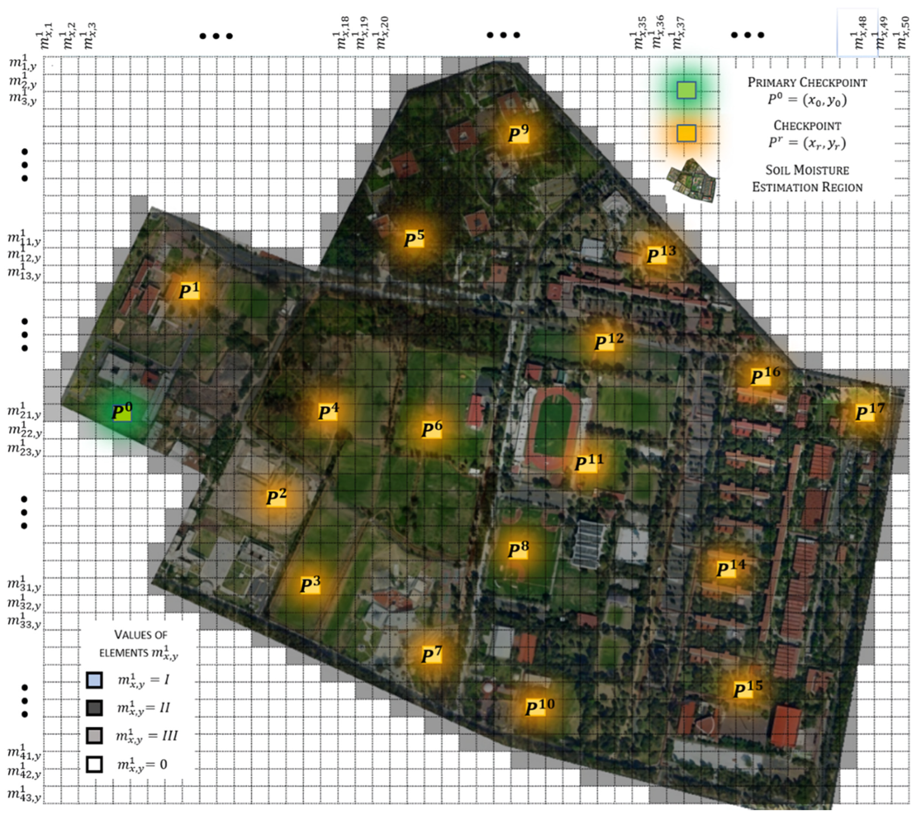
3.1.3. Checkpoint Location

The location $(x_r,y_r)$ of every checkpoint ($P^{r=\mathrm{1,2},\dots ,R}$) is used to identify the particular features of the sector where the checkpoint is located. The locations of the checkpoints shown in the region depicted in Figure 4 are included in Appendix A. During the model design stage, the next conditions define the checkpoint set: each landscape feature must predominate in at least one checkpoint, and checkpoints must allow for testing of the adjustment model at different lengths from the primary checkpoint $P^0$. During this model’s operation stage, every sector of the region is intended to be a checkpoint.

3.1.4. Weather Conditions Measured

The weather conditions measured ($C_{i=\mathrm{1,2},\dots ,I}^0)$ correspond to ($I=5)$ environmental variables measured at the primary checkpoint $(P^0).$ These weather conditions are necessary to estimate soil moisture with the point estimation model [35,45,46]. Temperature, rain, solar radiation, and wind speed are measured with an integrated sensor suite (ISS), and the integrated sensor suite calculates potential evapotranspiration. The values $v_{i=\mathrm{1,2},\dots ,I}$ presented in

Table 2. Measured weather conditions at the primary checkpoint ($\mathbf{I}=\mathbf{5}$).

${\mathit{C}}_{\mathit{i}=\mathrm{1,2},\dots ,\mathit{I}}^0$	Variable	Units	$\mathbf{Value} ({\mathit{v}}_{\mathit{i}}$)
$C_1^0$	Temperature $(T)$	$°\mathrm{C}$	18.1
$C_2^0$	Rain $(R)$	$\mathrm{m}\mathrm{m}$	0
$C_3^0$	Solar radiation $(Sr)$	$\mathrm{W}/{\mathrm{m}}^2$	890
$C_4^0$	Wind speed $(Ws)$	$\mathrm{K}\mathrm{m}/\mathrm{h}$	16
$C_5^0$	Evapotranspiration ($Et)$	$\mathrm{m}\mathrm{m}/\mathrm{d}$	5

correspond to measurements of a single day at primary checkpoint. Values corresponding to temperature ($C_1^0$), solar radiation ($C_3^0$), and wind speed ($C_4^0$) are the average records of the day, whereas values $v_{i=2}$ of rain ($C_2^0$) and potential evapotranspiration ($C_5^0$) are the cumulative measurements of the day.

3.2. Subzone Definition

In this stage, the landscape features (grassland, tree-covered areas, buildings areas, elevation, and spatial configuration) are identified through image processing of the satellite imagery. First, a space color conversion is executed from red, green, and blue (RGB) to the International Commission of Lighting (CIE L*a*b). Afterwards, a decorrelation is made as in [47]. 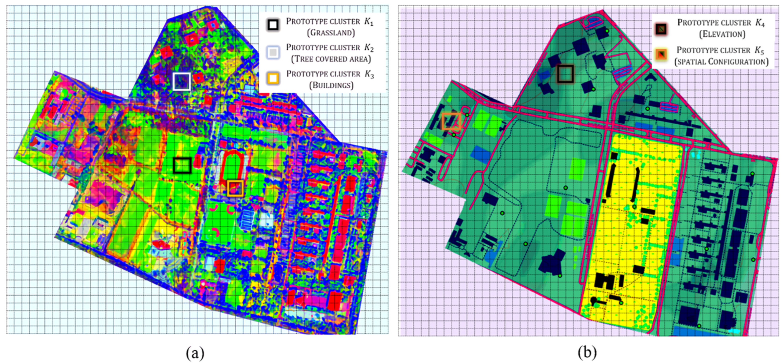For further information on image processing, refer to Appendix B. The image processing highlights the colors and shapes of the region so that a color segmentation of satellite images can be performed. In this paper, the two images from Figure 5a,b are processed images used to identify the landscape features. Grassland, tree-covered areas, and buildings are extracted from Figure 5a. Figure 5b is utilized to identify elevation and spatial configuration.

In color segmentation, a cluster ($K_{l=\mathrm{1,2},\dots ,L}$) is determined for each color band identified. Each cluster is associated with a landscape feature. In this work, the merging method is used for color segmentation. This method assumes that the features of all pixels are unlike at the beginning. Then, the algorithm K-means merges pixels according to the similarity criterion (Equation (1)) until no pixels remain merged [48]. Afterwards, the merged pixels are assigned to a cluster. Some pixels may not be assigned to a cluster, and a deficient color segmentation could mislead the weather conditions adjustment. When there is a high percentage of pixels not assigned ($\% PNA$), it is necessary to use an image with better resolution. In this paper, a $\%PNA<1.5$ is utilized based on the preliminary experimental analysis as described in Section 4.

$$G={\sum }_{l=1}^L{\sum }_{{\overrightarrow{a}}_dϵK_l}^{}{‖{\overrightarrow{a}}_d-{\overrightarrow{b}}_l‖}^2$$

(1)

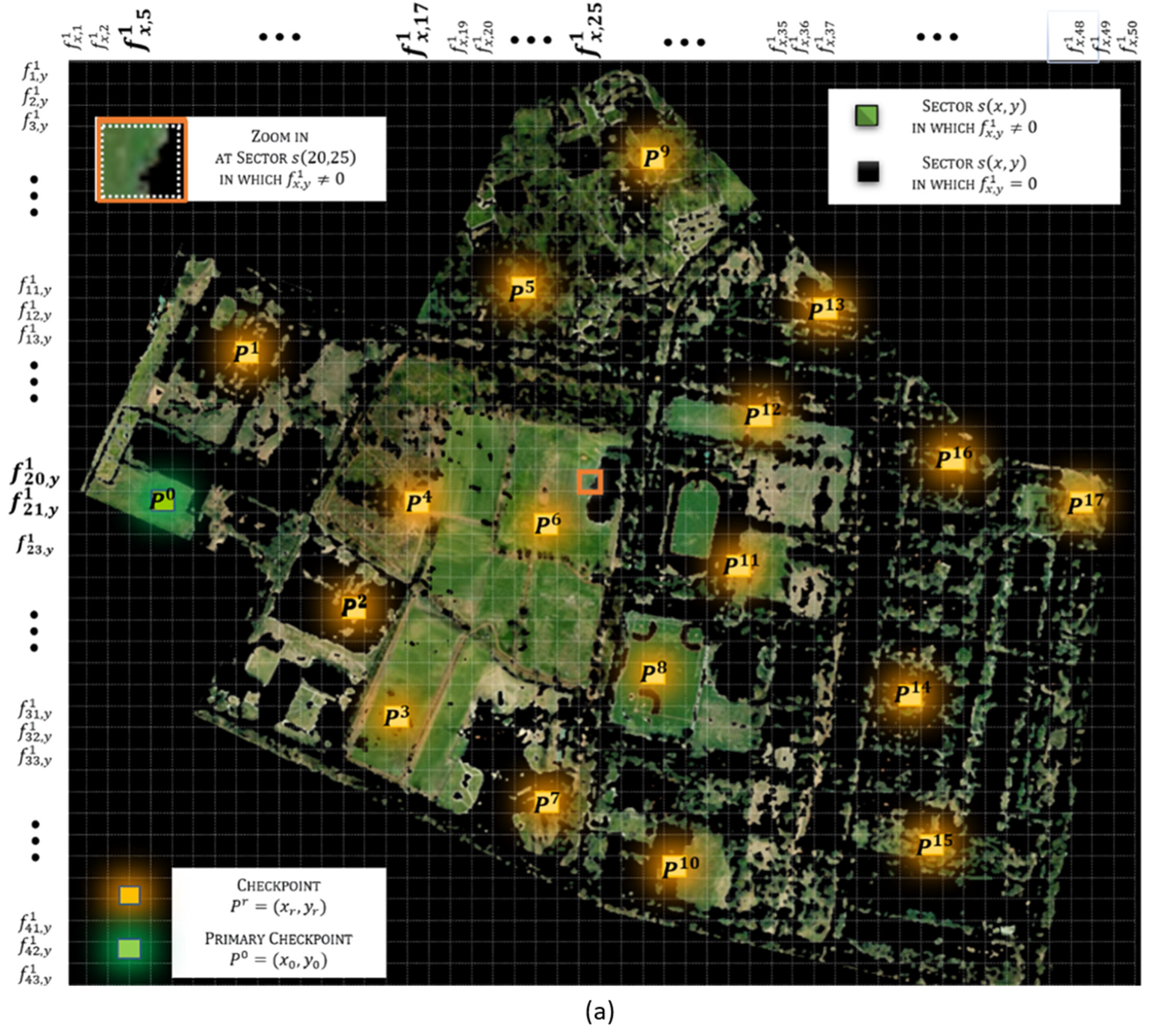
So far, the image is segmented pixel by pixel into clusters. Nonetheless, in the same way as the satellite image, the segmented images must be divided into sectors $(s\left(x,y\right)$) to obtain landscape matrices ($F^{l=\mathrm{1,2},\dots ,L}$). In feature matrices, the size of each landscape matrix is $X\times Y$. For matrices $F^{l=\mathrm{1,2},\mathrm{3,4}}$, each element ($f_{x,y}^l$) represents the number of pixels in a sector that belong to the cluster $K_l$ as shown in Figure 6a,b. The landscape matrices defined are the following:

• Matrix $F^{l=1}$ corresponds to grasslands.
• Matrix $F^{l=2}$ corresponds to tree-covered areas.
• Matrix $F^{l=3}$ corresponds to building areas.
• Matrix $F^{l=4}$ corresponds to elevation.
• Matrix $F^{l=5}$ corresponds to spatial configuration.

Figure 6. (a) Landscape matrix $F^1$ (grassland). (b) Landscape matrix $F^3$ (buildings).

Figure 6. (a) Landscape matrix $F^1$ (grassland). (b) Landscape matrix $F^3$ (buildings).

For instance, landscape matrices $F^1$ (grassland) and $F^3$(buildings) are depicted in Figure 6a,b, respectively. In this paper, each sector contains $858$ pixels. The value of the element $f_{\mathrm{20,25}}^1$ corresponding to sector $s\left(\mathrm{20,25}\right)$ is $f_{\mathrm{20,25}}^1=596$ because there are 596 pixels that belong to cluster $K_1$ (grassland).

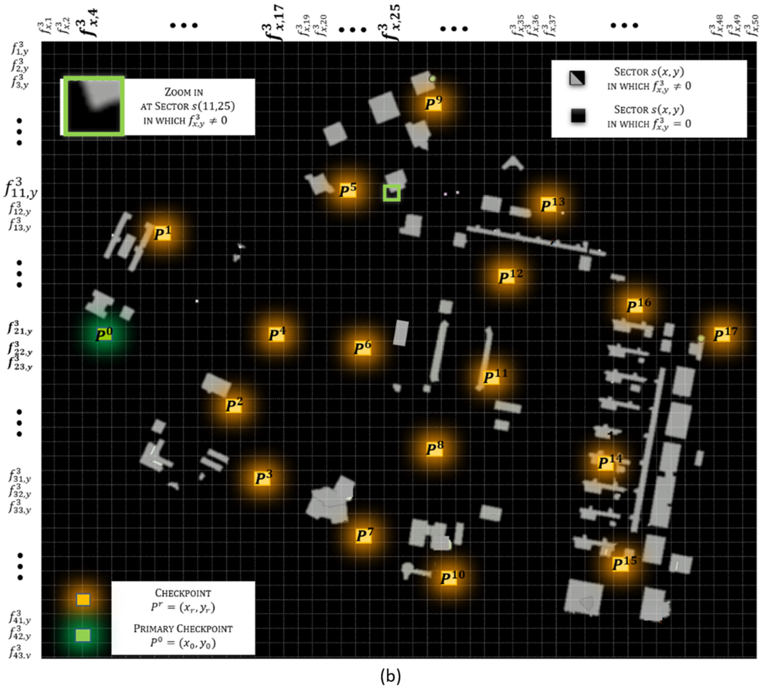
Furthermore, landscape matrix $F^{l=4}$ (elevation) is a particular case because its value not only refers to the number of pixels but also contains the elevation level of these pixels, e.g., element $f_{\mathrm{10,10}}^{l=4}=550,B$ defines that, at sector $s (x=10,y=10)$, there are 550 pixels that belong to elevation level $B$. Elevation levels are named as $A,B,C,\dots$, according to the region elevation model.

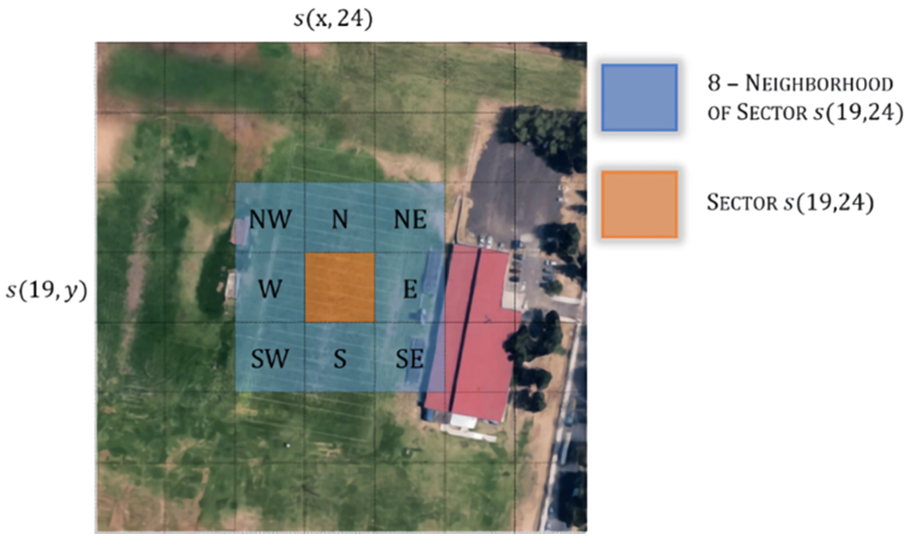
Moreover, for landscape matrix $F^{l=5}$ (spatial configuration), elements $f_{x,y}^{l=5}$ contain the number of pixels corresponding to the surrounding sectors’ buildings, roads, or natural barriers. A landscape feature analysis of the 8 neighborhoods of sector $s\left(x,y\right)$ is performed, e.g., sector $s(x=19,y=24)$ of the satellite image given in Figure 4 is shown in Figure 7, and the features of 8-neighborhood sectors ($N, NE, E, SE, S, SW, W, NW$) are analyzed. Neighbor sectors $N,S,SW$ present no buildings, roads, or natural barriers; meanwhile, neighbor sectors $NE,E,SE,W,NW$ denote the existence of buildings. The value of spatial configuration at sector $s\left(\mathrm{19,24}\right)$ is the addition of all pixels that belong to tree-covered areas ($F^2$) and buildings ($F^2$) in the neighbor sectors $N, NE, E, SE, S, SW, W, NW$. The spatial configuration is used by the adjustment model for modeling the interactions between the 8 neighborhoods and sector $s(x,y)$.

The weather conditions of a sector are not only influenced by its particular features but also by the particular features of the surrounding sectors ($N, NE, E, SE, S, SW, W, NW$).

3.3. Subzone Features Selection

The subzone features selection stage receives the landscape matrices ($F^{l=\mathrm{1,2},\dots ,L}$), the feature matrices ($M^{t=\mathrm{1,2},\dots ,T}$), and the checkpoint locations $(x_r,y_r)$. The data about landscape features ($f_{x,y}^l$) and soil and crop features ($m_{x,y}^t$) at the checkpoint location are selected from the matrices mentioned before.

These elements (grasslands, tree-covered areas, buildings areas, elevation, spatial configuration, soil type, crop type, and crop stage) compound the particular features (${\mathsf{\Phi }}^r(F^l,M^t,P^r))$of the checkpoint ($P^{r=\mathrm{0,1},\dots ,R })$as shown in Equation (2).

$${\mathsf{\Phi }}^r\left(F^l,M^t,P^r\right)=[f_{x_r,y_r}^1,f_{x_r,y_r}^2,\dots ,f_{x_r,y_r}^L,m_{x_r,y_r}^1,m_{x_r,y_r}^2,\dots ,m_{x_r,y_r}^T]$$

(2)

The following calculation example uses checkpoint $P^4$ with location $s(x_4=21,y_4=17)$ according to Figure 4 and

Table A1. Checkpoint location $s(x_r,y_r$).

Checkpoint ${\mathit{P}}^{\mathit{r}=\mathrm{0,1},\dots ,\mathit{R}}$	$\mathbf{Location} ({\mathit{x}}_{\mathit{r}},{\mathit{y}}_{\mathit{r}})$	Checkpoint ${\mathit{P}}^{\mathit{r}=\mathrm{0,1},\dots ,\mathit{R}}$	$\mathbf{Location} ({\mathit{x}}_{\mathit{r}},{\mathit{y}}_{\mathit{r}})$
$P^0$	(21,5)	$P^9$	(5,28)
$P^1$	(14,9)	$P^{10}$	(38,29)
$P^2$	(26,14)	$P^{11}$	(24,32)
$P^3$	(31,16)	$P^{12}$	(17,33)
$P^4$	(21,17)	$P^{13}$	(12,36)
$P^5$	(11,22)	$P^{14}$	(30,40)
$P^6$	(22,23)	$P^{15}$	(37,41)
$P^7$	(35,23)	$P^{16}$	(19,42)
$P^8$	(29,28)	$P^{17}$	(21,48)

. The particular features ${\mathsf{\Phi }}^4\left(F^4,M^4,P^4\right)$ of this test checkpoint, shown in Equation (3), are selected as defined in Equation (2), and their values are described in Equation (4). There are 818 pixels corresponding to $F^1$ (grassland) at checkpoint $P^4$, 17 pixels corresponding to $F^2$ (tree-covered areas), and so on.

$${\mathsf{\Phi }}^4\left(F^4,M^4,P^4\right)=[f_{\mathrm{21,17}}^1,f_{\mathrm{21,17}}^2,f_{\mathrm{21,17}}^3,f_{\mathrm{21,17}}^4,f_{\mathrm{21,17}}^5,m_{\mathrm{21,17}}^1,m_{\mathrm{21,17}}^2,m_{\mathrm{21,17}}^3]$$

(3)

$${\mathsf{\Phi }}^4\left(F^4,M^4,P^4\right)=[818,17,17,(858/A),121,(858/II),(858/1),(858/1)]$$

(4)

Notation ${\varphi }_{e=\mathrm{1,2},\dots ,E}^r$ shown in Equation (5) is used to denote particular features expressed as a percentage so that the level of each feature can be identified more easily.

$${\mathsf{\Phi }}^r\left(F^l,M^t,P^r\right)=\left[{\varphi }_{e=1}^r,{\varphi }_{e=2}^r,\dots ,{\varphi }_{e=L}^r,{\varphi }_{e=L+1}^r,{\varphi }_{e=L+2}^r,\dots ,{\varphi }_{e=E}^r\right];E=L+T$$

(5)

For instance, in Equation (6), the particular features from Equation (4) are expressed as a percentage, as defined in Equation (5). Equation (6) indicates that, at the test checkpoint, $95.338\%$ of the pixels correspond to grassland, $1.9813\%$ correspond to tree covered areas, and so on.

$${\mathsf{\Phi }}^4\left(F^4,M^4,P^4\right)=[95.338,1.9813,1.9813,(100/A),1.848,(100/II),(100/1),(100/1)]$$

(6)

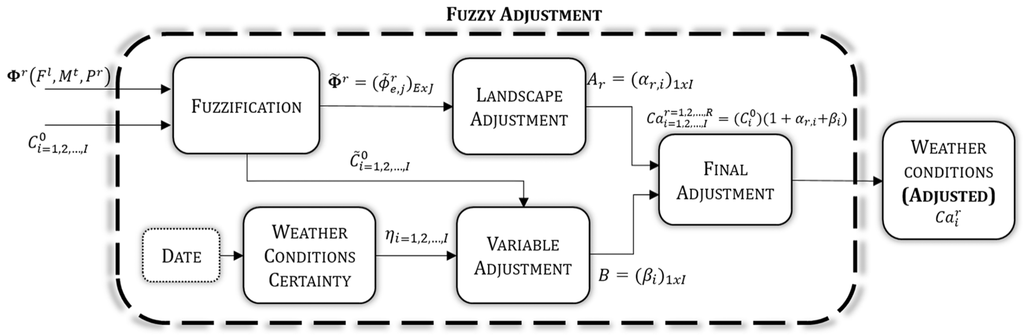
3.4. Fuzzy Adjustment

The fuzzy adjustment stage is depicted in Figure 8. This stage receives the particular features (from the previous stage) and the weather conditions measured (from inputs), and both are fuzzified.

Two fuzzy inference systems (landscape adjustment and variable adjustment) are performed to obtain the adjustment factors: steady$({A_{r=\mathrm{1,2},\dots ,R}}_{ })$ and variable $(B)$. Both adjustment factors determine the weather conditions adjusted (${Ca}_i^r$).

3.4.1. Fuzzification

The particular features and weather conditions measured are fuzzified using membership functions with the triangle form defined in Equation (7), L form defined in Equation (8), and gamma form defined in Equation (9) [49].

$${{\mu }_{\mathsf{\Delta }}}_{}\left(v\right)=\left\{\begin{array}{c}\frac{v-f}{g-f}, f\le v<g\\ \frac{h-v}{h-g}, g\le v\le h\\ 0, otherwise\end{array}\right.$$

(7)

$${\mu }_{\mathsf{\Gamma }}\left(v\right)=\left\{\begin{array}{cc}0;& v<f\\ \frac{v-f}{g-f};& f\le v<g\\ 1;& g\le v\end{array}\right.$$

(8)

$${\mu }_L\left(v\right)=\left\{\begin{array}{cc}1;& v<f\\ \frac{g-v}{g-f};& f\le v<g\\ 0;& g\le v\end{array}\right.$$

(9)

Each measured weather condition is fuzzified with five linguistic values (lower, low, medium, high, and higher) so that, by the time fuzzification is applied, each weather condition (temperature, rain, solar radiation, wind speed, and evapotranspiration) turns into a fuzzy weather condition vector $({\tilde{C}}_i^0\left(v_i\right))$, where $v_i\in V_i$. $v_i$ is the value of the weather condition $C_i^0$ and $V_i$ is the universe of discourse defined in

Table 3. Universe of the discourse of all measured weather conditions $C_{i=\mathrm{1,2},\dots ,I}^0$.

$\mathbf{Weather} \mathbf{Condition} ({\mathit{C}}_{\mathit{i}}^0)$	Variable	$\mathbf{Universe} \mathbf{of} \mathbf{Discourse} ({\mathit{V}}_{\mathit{i}}$)
$C_1^0$	Temperature $(°\mathrm{C})$	$V_1=\left[0, 40\right]$
$C_2^0$	Rain $(\mathrm{mm})$	$V_2=\left[0, 25\right]$
$C_3^0$	Solar Radiation $(\mathrm{W}/{\mathrm{m}}^2)$	$V_3=\left[0, 1250\right]$
$C_4^0$	Wind Speed $(\mathrm{km}/\mathrm{h})$	$V_4=\left[0, 50\right]$
$C_5^0$	Evapotranspiration ($\mathrm{mm}/\mathrm{d})$	$V_5=\left[0, 10\right]$

. Each fuzzy weather condition vector is composed of five elements (${\tilde{c}}_{i,j}^0| j=\mathrm{1,2},\dots ,J$) as defined in Equations (10)–(14).

$${\tilde{\mathit{C}}}_{\mathbf{1}}^{\mathbf{0}}(v_i)=\left\{{\tilde{c}}_{\mathrm{1,1}}^0,{\tilde{c}}_{\mathrm{1,2}}^0,\cdots ,{\tilde{c}}_{\mathrm{1,5}}^0\right\}$$

(10)

$${\tilde{\mathit{C}}}_{\mathbf{2}}^{\mathbf{0}}(v_i)=\left\{{\tilde{c}}_{\mathrm{2,1}}^0,{\tilde{c}}_{\mathrm{2,2}}^0,\cdots ,{\tilde{c}}_{\mathrm{2,5}}^0\right\}$$

(11)

$${\tilde{\mathit{C}}}_{\mathbf{3}}^{\mathbf{0}}\left(v_i\right)=\left\{{\tilde{c}}_{\mathrm{3,1}}^0,{\tilde{c}}_{\mathrm{3,2}}^0\cdots ,{\tilde{c}}_{\mathrm{3,5}}^0\right\}$$

(12)

$${\tilde{\mathit{C}}}_{\mathbf{4}}^{\mathbf{0}}(v_i)=\left\{{\tilde{c}}_{\mathrm{4,1}}^0,{\tilde{c}}_{\mathrm{4,2}}^0,\cdots ,{\tilde{c}}_{\mathrm{4,5}}^0\right\}$$

(13)

$${\tilde{\mathit{C}}}_{\mathbf{5}}^{\mathbf{0}}(v_i)=\left\{{\tilde{c}}_{\mathrm{5,1}}^0,{\tilde{c}}_{\mathrm{5,2}}^0,\cdots ,{\tilde{c}}_{\mathrm{5,5}}^0\right\}$$

(14)

Elements of the fuzzy weather condition vector are associated with a linguistic variable $j$. The linguistic labels used are the following:

• $j=1$ Lower level of weather condition $C_i^0$.
• $j=2$ Low level of weather condition $C_i^0$.
• $j=3$ Medium level of weather condition $C_i^0$.
• $j=4$ High level of weather condition $C_i^0$.
• $j=5$ Higher level of weather condition $C_i^0$.

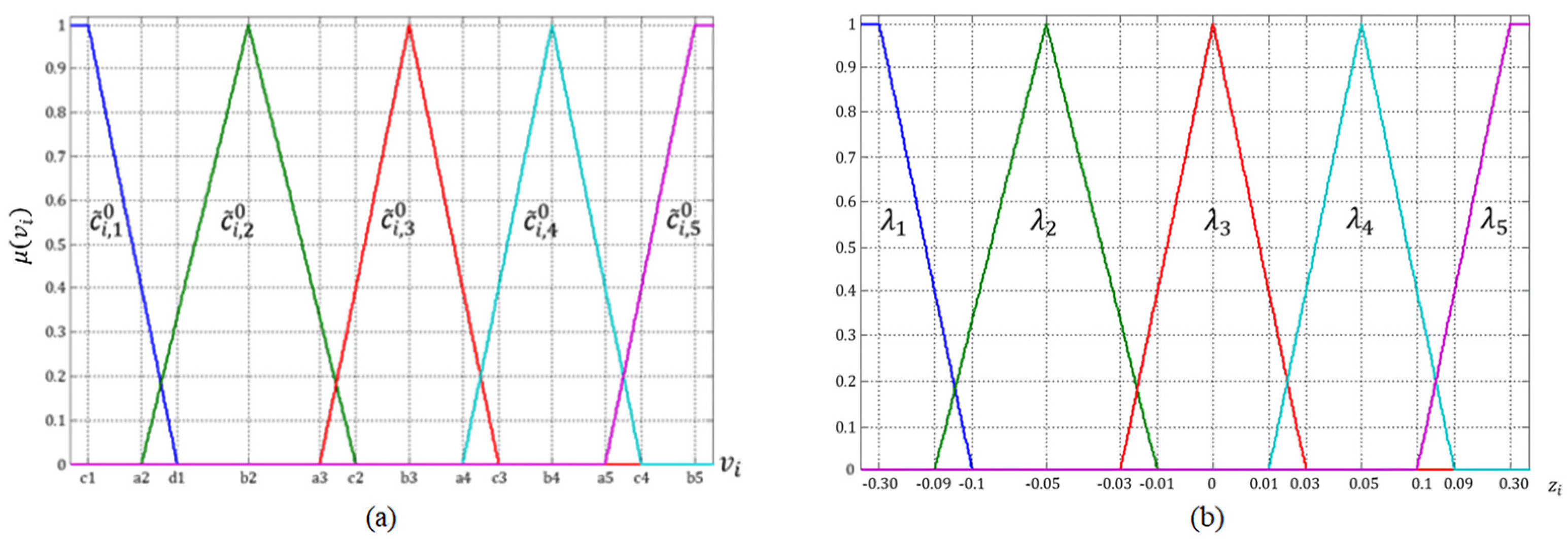
In the same way, each element is related to a membership function of the form defined in Equations (7)–(9). Element ${\tilde{c}}_{i,1}^0| i=\mathrm{1,2},\dots ,I$ comes from the gamma shape membership function, whereas element ${\tilde{c}}_{i,5}^0| i=\mathrm{1,2},\dots ,I$ is L shape membership function. Elements ${\tilde{c}}_{i,j}^0| i=\mathrm{1,2},\dots ,I;j=\mathrm{2,3},4$ are triangle membership functions. The linguistic values and the membership functions are set based on the experimental analysis’s best results during the adjustment model’s development stage. The parameters determined for the region shown in Figure 4 are described in

Table 4. Membership functions parameters of weather conditions $C_{i=\mathrm{1,2},\dots ,I}^0$.

Linguistic Value	Function	${\mathit{C}}_{\mathit{i}=1}^0$	${\mathit{C}}_{\mathit{i}=2}^0$	${\mathit{C}}_{\mathit{i}=3}^0$	${\mathit{C}}_{\mathit{i}=4}^0$	${\mathit{C}}_{\mathit{i}=5}^0$
Lower	L	(0, 6)	$\left(0, 1\right)$	$\left(0, 140\right)$	$\left(0, 6\right)$	$\left(0, 1\right)$
Low	Triangle	(5, 10, 15)	$\left(0.8, 1.5, 2.2\right)$	$\left(120, 180, 240\right)$	$\left(4 ,8, 12\right)$	$\left(0.6, 1.6, 2.6\right)$
Medium	Triangle	(14, 20, 24)	$\left(1.9, 3.8, 6\right)$	$\left(220, 400, 580\right)$	$\left(10, 15, 20\right)$	$\left(2.3, 3.3, 4.3\right)$
High	Triangle	(22, 27, 32)	$\left(5, 8, 12\right)$	$\left(560, 700, 840\right)$	$\left(18, 25, 32\right)$	$\left(4, 5, 6\right)$
Higher	Gamma	(30, 35)	$\left(10, 18\right)$	$\left(800, 1000\right)$	$\left(30, 35\right)$	$\left(5.7, 6.7\right)$

and depicted in Figure A1a. Suppose that the adjustment model is implemented in another region; in that case, the entire process followed in the experiments developed in this paper must be replicated to obtain the parameters of the new region. However, the membership functions and linguistic labels’ type and number remain the same. The membership functions’ parameters presented in this document can be utilized, but they must be modified according to the best results of the new experimental analysis.

For example, the weather conditions measured from Table 2 and their parameters (Table 4) are utilized to obtain the values of fuzzy weather condition vectors of Equations (15)–(19).

$${\tilde{\mathit{C}}}_{\mathbf{1}}^{\mathbf{0}}(18.1)=\left\{\mathrm{0,0},\mathrm{0.82,0},0\right\}$$

(15)

$${\tilde{\mathit{C}}}_{\mathbf{2}}^{\mathbf{0}}(0)=\left\{\mathrm{1,0},\mathrm{0,0},0\right\}$$

(16)

$${\tilde{\mathit{C}}}_{\mathbf{3}}^{\mathbf{0}}(890)=\left\{\mathrm{0,0},\mathrm{0,0},0.3889\right\}$$

(17)

$${\tilde{\mathit{C}}}_{\mathbf{4}}^{\mathbf{0}}(16)=\left\{\mathrm{0,0},\mathrm{0.8,0},0\right\}$$

(18)

$${\tilde{\mathit{C}}}_{\mathbf{5}}^{\mathbf{0}}(5)=\left\{\mathrm{0,0},\mathrm{0,1},0\right\}$$

(19)

Moreover, to fuzzify particular features defined in Equation (5), it is necessary to compare the differences between specific features at the primary checkpoint ${\mathsf{\Phi }}^0(F^l,M^t,P^0)$and particular features at each checkpoint $({\mathsf{\Phi }}^r(F^l,M^t,P^r))$. This comparison allows one to determine the variations in the weather conditions derived from landscape influence. For example, according to the checkpoint set from Figure 4 and Table A1, and comparing the tree-covered area (a particular feature ${\varphi }_{e=5}^0)$, the primary checkpoint is not a tree-covered area, while checkpoint $P^{5 }$ is. So, temperature ($C_1^0$) measured at the primary checkpoint can be higher than temperature ($C_1^5$) at $P^{5 }$ because trees reduce sun exposure (solar radiation $C_3^5$) and cool air temperature ($C_1^5$). However, despite this fact, if there are high winds (wind speed $C_4^0$) at primary checkpoint, air temperature ($C_1^0$) can be reduced because of the wind chill factor; meanwhile, at $P^{5 },$trees block high winds ($C_4^5$) and no wind chill is present at this location. As a consequence, the temperature measured ($C_1^0$) can be the same as temperature ($C_1^5$) at $P^{5 }$.

The comparison (${\mathsf{\Phi }}^{0,r})$ between particular features is a difference as shown in Equation (20).

$${{\mathsf{\Phi }}^{0,r}={\mathsf{\Phi }}^0\left(F^l,M^t,P^0\right)-\mathsf{\Phi }}^r\left(F^l,M^t,P^r\right)=[{\varphi }_{e=1}^0-{\varphi }_{e=1}^r,{\varphi }_{e=2}^0-{\varphi }_{e=2}^r,\cdots ,{\varphi }_{e=E}^0-{\varphi }_{e=E}^r]$$

(20)

For instance, the particular features at the primary checkpoint are shown in Equation (21) and particular features at the test checkpoint in Equation (6). The comparison (${\mathsf{\Phi }}^{\mathrm{0,4}})$ is executed using Equation (20); the result is shown in Equations (22) and (23).

$${\mathsf{\Phi }}^0\left(F^l,M^t,P^0\right)=[100,0,0,(100/A),22.76,(100/II),(100/1),(100/1)]$$

(21)

$$\begin{gathered} {\mathsf{\Phi }}^{\mathrm{0,4}}=[100-95.338,0-\mathrm{1.9813,0}-1.9813,(100-100)/A,22.76-1.848, \\ (100-100)/I,(100-100)/1,(100-100)/1] \end{gathered}$$

(22)

$${\mathsf{\Phi }}^{\mathrm{0,4}}=[4.662,-1.9813,-1.9813,(0/A),20.86,(0/I),(0/1),(0/1)]$$

(23)

The comparison of particular features is fuzzified with a similar process as that followed to fuzzify the weather conditions measured. The comparison denotes whether each particular feature (${\varphi }_e^0)$ at the primary checkpoint is lower, equal, or higher than the particular feature (${\varphi }_e^r)$ at any checkpoint ($P^r).$ Hence, the linguistic labels used to fuzzify the particular features comparison are the following:

• $j=1$ ${\varphi }_e^0$ is lower than ${\varphi }_e^r$.
• $j=2$ ${\varphi }_e^0$ is equal to ${\varphi }_e^r$.
• $j=3$ ${\varphi }_e^0$ is higher than ${\varphi }_e^r$.

When fuzzified, the comparison of features turns into the fuzzy particular feature matrix (${\tilde{\mathsf{\Phi }}}^r)$, defined in Equation (24). This matrix is the fuzzified comparison of features at the primary checkpoint and any other checkpoint. As the comparison of features is executed individually, a fuzzy particular feature matrix is obtained for each checkpoint. The matrix rows represent each element of the comparison vector, and the columns contain the fuzzy values (${\tilde{\varphi }}_{e,j}^r | j=\mathrm{1,2},\dots ,J)$ obtained with the membership ($j=\mathrm{1,2},\dots ,J$).

$${\tilde{\mathsf{\Phi }}}^r=\left[\begin{array}{ccc}{\tilde{\varphi }}_{\mathrm{1,1}}^r& {\tilde{\varphi }}_{\mathrm{1,2}}^r& {\tilde{\varphi }}_{\mathrm{1,3}}^r\\ {\tilde{\varphi }}_{\mathrm{2,1}}^r& {\tilde{\varphi }}_{\mathrm{2,2}}^r& {\tilde{\varphi }}_{e,3}^r\\ ⋮& ⋮& ⋮\\ {\tilde{\varphi }}_{\mathrm{5,1}}^r& {\tilde{\varphi }}_{\mathrm{5,2}}^r& {\tilde{\varphi }}_{\mathrm{5,3}}^r\end{array}\right]$$

(24)

The universe of discourse is the same for all elements of the comparison, and it is expressed in a percentage as $U=[-100, 100]$. Meanwhile, the membership functions are also those defined in Equations (7)–(9).

Elements ${\tilde{\varphi }}_{e,1}^r | e=\mathrm{1,2},\dots ,E$ come from gamma shape membership function, elements ${\tilde{\varphi }}_{e,3}^r | e=\mathrm{1,2},\dots ,E$ are L shape membership functions, and elements ${\tilde{\varphi }}_{e,2}^r| e=\mathrm{1,2},\dots ,E$ are triangle shape membership functions.

The linguistic values and membership functions are set based on the experimental analysis’s best result during the adjustment model’s development stage. The parameters of a particular feature ${\varphi }_{e=1}^r$ (grassland) obtained for this region are shown in

Table 5. Membership functions of a particular feature ${\varphi }_{e=1}^0{-\varphi }_{e=1}^r$ (grassland).

Linguistic Value	Function Type	$\mathbf{Parameters} \mathbf{in} \mathbf{Percentage} (\mathit{f},\mathit{g},\mathit{h})$
Lower	L	(−60, −20)
Equal	Triangle	(−25, 0, 25)
Higher	Gamma	(20, 60)

; they are the same for all particular features.

For example, according to Equation (24), the fuzzy particular feature matrix of the test checkpoint (Equation (25)) is derived from fuzzifying the comparison of Equation (23) using the membership functions described in Table 5. The fuzzy particular feature matrix of Equation (25) highlights that particular features of the primary checkpoint and the test checkpoint are alike, so weather conditions are expected to be similar at both locations.

$${\tilde{\mathsf{\Phi }}}^4=\left[\begin{array}{ccc}0& 0.8152& 0\\ 0& 0.9615& 0\\ 0& 0.9615& 0\\ 0& 1& 0\\ 0& 0.5827& 0.0215\end{array}\right]$$

(25)

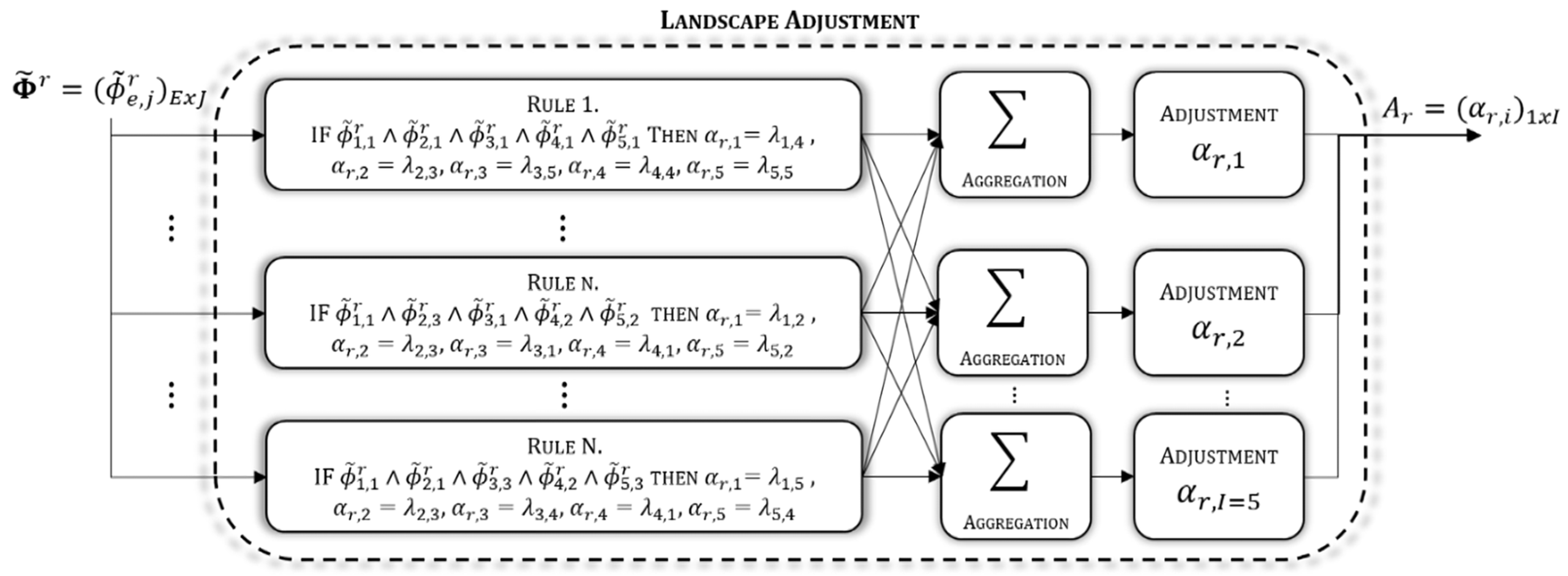
3.4.2. Landscape Adjustment

In the adjustment model, there is a stage that models the influence of particular features over the weather conditions. It is called the landscape adjustment and is depicted in Figure 9. As the particular features of each checkpoint can be different, a landscape adjustment is performed at each checkpoint. A fuzzy inference system is implemented in all the landscape adjustments. The results of every landscape adjustment are the steady factors; these are considered steady because they do not change while the particular features of the checkpoint remain the same. So, this adjustment does not need to be implemented each time a weather condition adjustment is made.

The input of the fuzzy inference system is the fuzzy particular features matrix of the checkpoint, and the outputs are the steady factors. Each steady factor (${\alpha }_{r,i}| i=\mathrm{1,2},\dots ,I$, where $I$ is the total of weather conditions) is divided into output sets (${\lambda }_{i,o} | o=\mathrm{1,2},\dots ,O,$ where $O=5$). The membership functions used for the output sets are of the form defined in Equations (7)–(9). The universe of discourse is $z_i\in Z$, $Z=[-\mathrm{1,1}]$. Each output membership represents a percentage of adjustment in each weather condition, as shown in

Table 6. Output’s (${\mathit{\alpha }}_{\mathit{r},\mathit{i}}$) membership functions.

$\mathbf{Output} \mathbf{Function} {\mathit{\lambda }}_{0=\mathrm{1,2},\dots ,\mathit{O}}$	Linguistic Label	Function Type	$\mathbf{Parameters} (\mathit{f},\mathit{g}) \mathit{o}\mathit{r} (\mathit{f},\mathit{g},\mathit{h})$
${\lambda }_{o,1}$	Low	L	(−0.3, −0.15)
${\lambda }_{o,2}$	Barely Low	Triangle	(−0.17, −0.1, −0.03)
${\lambda }_{\mathrm{0,3}}$	Null	Triangle	(−0.05, 0, 0.05)
${\lambda }_{o,4}$	Barely High	Triangle	(0.03, 0.1, 0.17)
${\lambda }_{o,5}$	High	Gamma	(0.15, 0.3)

. ${\lambda }_{i,1}$ is an L shape function, ${\lambda }_{o=\mathrm{2,3},4}$ are triangle functions, and ${\lambda }_{i,5}$ is a gamma shape function. The membership functions used for all steady factors $({\alpha }_{r,i}$) are defined in Table 6 and depicted in Figure A1b.

All rules are generated manually based on observation and expert knowledge. Adjusting membership functions and rule generation using automatic methods are outside this work’s scope. Rules $n=\mathrm{1,2},\dots ,N$, where $N=245$, are established and processed for modeling steady factors, as shown in Figure 9. The rules are established based on the effects of particular features on the weather conditions. Each rule inter-relates the fuzzy particular features (${\tilde{\varphi }}_{e,j}^r$) using the premise IF THEN. Furthermore, the rules remain the same for all the checkpoints. The rules are of the form: IF ${\tilde{\mathit{\varphi }}}_{\mathbf{1,3}}^{\mathit{r}}\wedge {\tilde{\mathit{\varphi }}}_{\mathbf{2,2}}^{\mathit{r}}\wedge {\tilde{\mathit{\varphi }}}_{\mathbf{3,2}}^{\mathit{r}}\wedge {\tilde{\mathit{\varphi }}}_{\mathbf{4,2}}^{\mathit{r}}\wedge {\tilde{\mathit{\varphi }}}_{\mathbf{5,2}}^{\mathit{r}}$ THEN ${\mathit{\alpha }}_{\mathbf{4,1}}={\mathit{\lambda }}_{\mathbf{1,4}}$, ${\mathit{\alpha }}_{\mathbf{4,2}}={\mathit{\lambda }}_{\mathbf{2,3}}$, ${\mathit{\alpha }}_{\mathbf{4,3}}={\mathit{\lambda }}_{\mathbf{3,4}}$, ${\mathit{\alpha }}_{\mathbf{4,4}}={\mathit{\lambda }}_{\mathbf{4,3}}$, ${\mathit{\alpha }}_{\mathbf{4,5}}={\mathit{\lambda }}_{\mathbf{5,4}}$, e.g., the previous rule corresponds to rule $n=41$ applied at the test checkpoint, and it can be interpreted as follows:

IF grassland is Higher (${\tilde{\varphi }}_{\mathrm{1,3}}^4$) and tree-covered area is Equal (${\tilde{\varphi }}_{\mathrm{2,2}}^4$) and building area is Equal $({\tilde{\varphi }}_{\mathrm{3,2}}^4)$ and elevation is Equal ${(\tilde{\varphi }}_{\mathrm{4,2}}^4)$ and spatial configuration is Equal (${\tilde{\varphi }}_{\mathrm{5,2}}^r$) THEN adjustment factor for temperature $({\alpha }_{\mathrm{4,1}}$) is Barely High (${\lambda }_{\mathrm{1,4}}$), adjustment factor for rain $({\mathit{\alpha }}_{\mathbf{4,2}}$) is Null (${\lambda }_{\mathrm{2,3}}$), adjustment factor for solar radiation $({\mathit{\alpha }}_{\mathbf{4,3}}$) is High (${\lambda }_{3.4}$), adjustment factor for wind speed $({\mathit{\alpha }}_{\mathbf{4,4}}$) is Null (${\lambda }_{\mathrm{4,3}}$); meanwhile, adjustment factor for evapotranspiration $({\mathit{\alpha }}_{\mathbf{4,5}}$) is Barely High (${\lambda }_{\mathrm{5,4}}$).

The rule definition matrices $(H^L={\left(h_{n,e}^L\right)}_{NxE}$, where elements $h_{n,e}^L | e=\mathrm{1,2},\dots ,E$) determine the fuzzy particular features utilized for assessing each rule $n$of checkpoint $P^r$ as described in Equation (26). The rows refer to the number of rules and the columns to the fuzzy particular feature.

$$h_{n,e}^L=\left\{\begin{array}{cc}1& if {\tilde{\varphi }}_{e,j}^r is not used in rule n\\ {\tilde{\varphi }}_{e,j}^r& otherwise\end{array}\right.$$

(26)

Moreover, $S^L={\left(s_{n,i}^L\right)}_{NxI}$ is the output definition matrix for landscape adjustment of checkpoint $P^r$. Elements $s_{n,i}^L$ denote which output membership function (low, barely low, null, barely high, high) represents the output ${\alpha }_{r,i}$ according to rule $n$. The rows refer to the number of rules and the columns to the output membership functions of the steady factor. The implication of the rule $n$ is denoted by the word “and”, defined as the function min. The result of the assessment $({\tau }_{n,o}^i)$ is obtained as defined in Equation (27).

$${\tau }_{n,o}^i=\left\{\begin{array}{cc}\hfill min\left(h_{n,1}^L,h_{n,2}^L,\dots ,h_{n,E}^L\right),& {\lambda }_{i,o}=s_{n,i}^L \hfill \\ \hfill 0,& {\lambda }_{i,o}\ne s_{n,i}^L\hfill \end{array}\right.$$

(27)

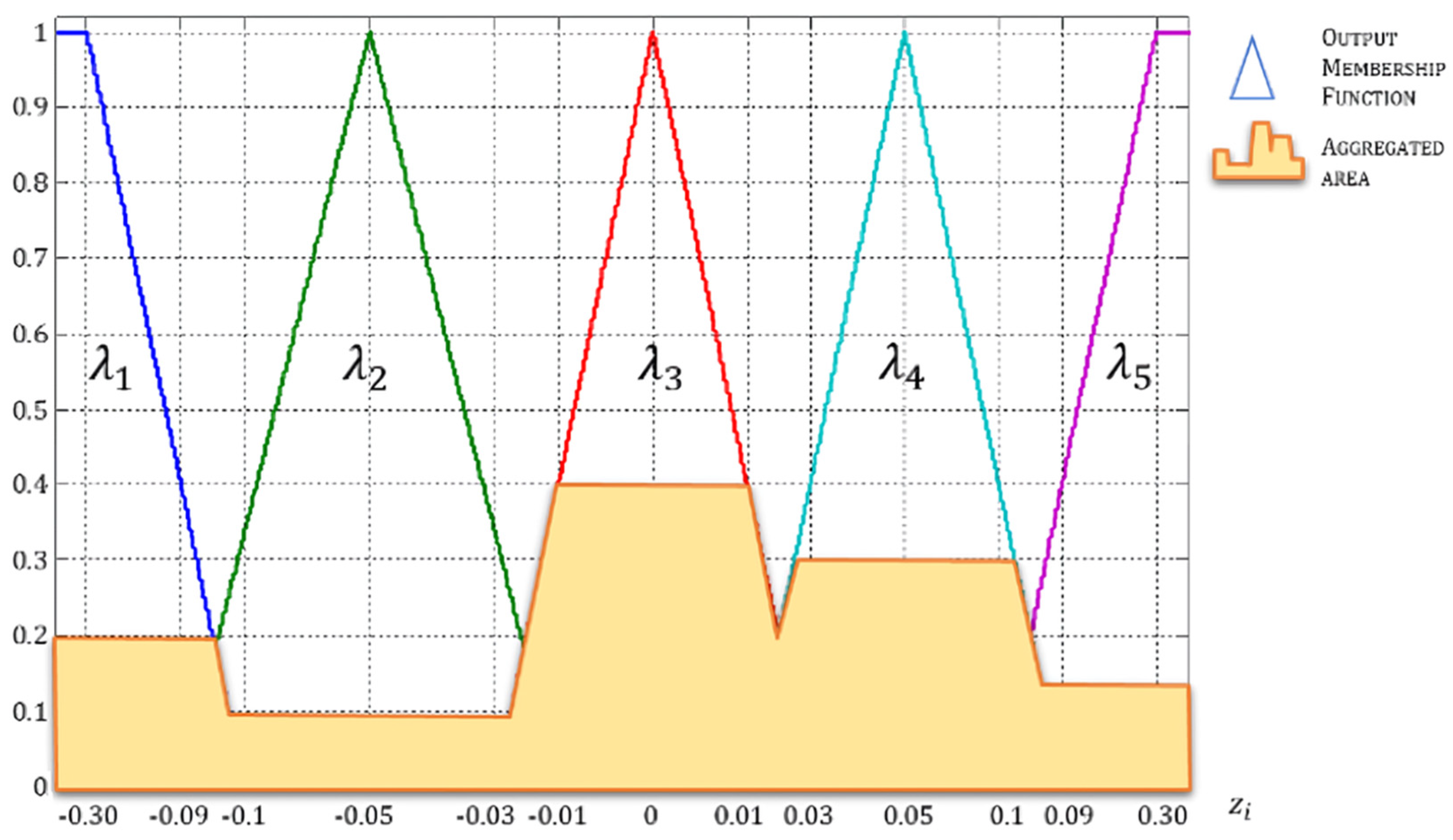
Afterwards, the results of the assessments are sent to the aggregation process. The aggregation delimits the output functions (${\lambda }_{i,o})$ and aggregates them in a single area, as shown in Figure A2. The method used for aggregation is the maximum defined in Equation (28), where $T_{ }^i$ is the aggregated function for output ${\alpha }_{r,i}$.

$$T^i=max({\tau }_{1,o}^i,{\tau }_{2,o}^i,\dots ,{\tau }_{N,o}^i)|o=\mathrm{1,2},\dots ,O; i=\mathrm{1,2},\dots ,I$$

(28)

For instance, using Equation (27), the rule definition matrix ($H^L$), and the output definition matrix ($S^L$), the rule $n=41$ for the steady factor of temperature (${\alpha }_{\mathrm{4,1}}$) is assessed as in Equation (29). The result of rule (${\tau }_{\mathrm{41,4}}^1$) is assigned to the output membership function barely high (${\lambda }_{\mathrm{1,4}}$). The same process is applicable for the $N$ rules as well as for the $I$ outputs.

$${\tau }_{\mathrm{41,4}}^1=min\left({\tilde{\varphi }}_{\mathrm{1,3}}^4,{\tilde{\varphi }}_{\mathrm{2,2}}^4,{\tilde{\varphi }}_{\mathrm{3,2}}^4,{\tilde{\varphi }}_{\mathrm{4,2}}^4,{\tilde{\varphi }}_{\mathrm{5,2}}^4\right)=\mathit{min}\left(\mathrm{0.2670,0.9615,0.9615,1},0.5827\right)=0.267$$

(29)

Afterwards, the aggregated function ($T^i)$ is defuzzfied to obtain the steady factor $({\alpha }_{r,i}$) of each weather condition $(C_i^0)$. The defuzzification method used in this paper is the centroid method defined in Equation (30).

$${\alpha }_{r,i}=\frac{\sum _{l=0}^L{T}_l^i{z}_l}{\sum _{l=0}^L{T}_l^i}$$

(30)

All the steady factors (${\alpha }_{r,i}$) defuzzfied conform the steady factors vector presented in Equation (31). The steady factors vector ($A_r)$ adjusts each weather condition measured according to the particular features of checkpoint $P^r$.

$$A_r=\left[{\alpha }_{r,1,}{\alpha }_{r,2},\dots ,{\alpha }_{r,I}\right]$$

(31)

For example, the steady factors vector ($A_4)$ for the test checkpoint is obtained according to Equation (31) and is shown in Equation (32). In this case, the steady factor for temperature (${\alpha }_{\mathrm{4,1}})$ indicates that, according to the features at the test checkpoint, the temperature must be modified to $0.0544$, i.e., the adjustment is about $+5.4\%$ of its value.

$$A_4=[\mathrm{0.0544,0.0544,0.0544},-\mathrm{0.004,0.5249}]$$

(32)

3.4.3. Weather Conditions Certainty

Sometimes, weather conditions can vary in two near locations within a region, i.e., sometimes, it can be raining at the initial location where the observer is, but when the observer moves from the initial location to another a few meters ahead, it cannot be raining. This situation is caused by different events [50]. However, one of the most relevant is the season of the year, which increases the certainty that a weather condition is similar in most locations within a region of interest, e.g., it is more conceivable that, in the rainy season, it is raining in the whole region. Therefore, a certainty distribution function, which depends on the date, can describe the certainty of the weather condition replication in a region. Moreover, not all the weather conditions considered in this work present the uncertainties described above, e.g., temperature, which remains homogeneous in a specific region if the variations due to landscape features are not considered.

Consequently, in the variable adjustment, the date and a certainty distribution function are utilized to determine the weather conditions certainty ${\eta }_{i=\mathrm{1,2},\dots ,I}$. Rain $(C_{i=2}^0)$, solar radiation $(C_{i=3}^0)$, wind speed $(C_{i=4}^0)$, and evapotranspiration $(C_{i=5}^0)$ are expected to be affected by the date (season of the year), and their distribution function is defined in Equation (33). Weather conditions certainty of temperature $(C_{i=1}^0)$ is not considered to be influenced by the date (season of the year).

$${\eta }_i=e^{\frac{-{(d-g)}^2}{2f^2}}$$

(33)

In Equation (33), $d$ is the month, and $(f,g)$ are the function parameters: $f$ indicates rainy season deviation expressed in months, and $g$ defines the month of peak rainy season. This certainty distribution function ${\eta }_{i=\mathrm{2,3},5}$ corresponds to a Gaussian bell, which increases the certainty ${\eta }_{i=\mathrm{2,3},5}$ during the rainy season. The certainty distribution function parameters $(f,g)$ for certainties ${\eta }_{i=\mathrm{2,3},5}$ (rain, solar radiation, and evapotranspiration) are $(\mathrm{3,7})$; meanwhile, for certainty ${\eta }_{i=4}$ (wind speed), the parameters are $(\mathrm{1,10})$. The weather conditions were measured at different checkpoints during the development stage of the adjustment model. The measurement records allow for the definition of parameters $\left(f,g\right)$ that best describe the certainty distribution function. If the adjustment model is applied in another region, the parameters $\left(f,g\right)$ presented in this paper can be utilized, although they can be modified to adapt appropriately to the features of the new region.

For example, certainty ${\eta }_1$ (temperature) is always considered as ${\eta }_1=1$. Certainties ${\eta }_{i=\mathrm{2,3},\mathrm{4,5}}$ are calculated with Equation (33) using the parameters $(f,g)$ above defined for each weather condition. The certainties ${\eta }_{i=\mathrm{2,3},\mathrm{4,5}}$ during August $(d=8)$, a rainy season month, are shown in Equations (34) and (35).

$${\eta }_2={\eta }_3={\eta }_5=e^{\frac{-{(8-7)}^2}{2{(3)}^2}}=0.9460$$

(34)

$${\eta }_4=e^{\frac{-{(8-10)}^2}{2{(1)}^2}}=0.1353$$

(35)

3.4.4. Variable Adjustment

The variable adjustment models the interactions among weather conditions. The variable adjustment also implements a fuzzy inference system. The result is the variable factor ($B$). In this adjustment, first, the weather condition certainty (${\eta }_{i=\mathrm{1,2},\dots ,I})$ is used to weigh the fuzzy weather conditions (${\tilde{\mathit{C}}}_{\mathit{i}}^{\mathbf{0}}$) obtained in Section 3.4.3. If the certainty ${\eta }_i$ is high, then it is more likely that the weather condition is similar in the whole region. Therefore, it is more important to model its interactions $({\tilde{\mathit{C}}}_{\mathit{i}}^{\mathbf{0}})$. For example, if the rain certainty is ${\eta }_2=0.98$, it is more feasible that the rain value measured at the primary checkpoint is similar at the other checkpoints, with a high certainty value; if it is raining at the primary checkpoint, it is more likely that it is raining throughout the region. Consequently, rainfall value should be considered more relevant for modeling the variations in weather conditions caused by the rain effects over the other weather conditions, such as the decrease in temperature or solar radiation. Weather conditions are weighed by a product of fuzzy weather conditions and their certainty of replication.

The variable factor vector ($B$) is formed of individual variable factors (${\beta }_i | i=\mathrm{1,2},\dots ,I$). The output membership functions $({\mathsf{\omega }}_{i,o=\mathrm{1,2},\dots ,O}$, where $O=5$) of the variable factors are also associated with linguistic labels, which refer to the required adjustment in a percentage of the weather conditions measured. Also, output functions ${\mathsf{\omega }}_{i,1}$ are $L$ shape functions as defined in Equation (7), ${\mathsf{\omega }}_{i,2}$ are triangle shape functions as defined in Equation (8), and ${\mathsf{\omega }}_{i,3}$ are gamma shapes as in Equation (9). The output membership functions are defined for $z_i\in Z$, where $Z=\left[\mathrm{0,2}\right]$ is the universe of discourse. The output membership functions for all variable factors are described in

Table 7. Output’s (${\mathit{\beta }}_{\mathit{i}}$) membership functions.

$\mathbf{Output} \mathbf{Function} {\mathit{\omega }}_{0=\mathrm{1,2},\dots ,\mathit{O}}$	Linguistic Label	Function	$(\mathit{f},\mathit{g}) \mathit{o}\mathit{r} (\mathit{f},\mathit{g},\mathit{h})$
${\mathsf{\omega }}_{\mathrm{i},1}$	Low	L	(0.8, 0.85)
${\mathsf{\omega }}_{\mathrm{i},2}$	Barely Low	Triangle	(0.84, 0.9, 0.94)
${\mathsf{\omega }}_{\mathrm{i},3}$	Null	Triangle	(0.93, 1, 1.05)
${\mathsf{\omega }}_{\mathrm{i},4}$	Barely High	Triangle	(1.04, 1.1, 1.16)
${\mathsf{\omega }}_{\mathrm{i},5}$	High	Gamma	(1.15, 1.2)

; meanwhile, Figure A1b can be used to depict the shape of the output membership functions due to the similarity of both output membership function sets.

A similar procedure to that developed in Section 3.4.2 is followed in this adjustment. However, the variable adjustment does not depend on the particular features of a checkpoint, so this adjustment is the same for any checkpoint; the same variable factor vector is utilized. Nonetheless, this adjustment is executed each time a weather conditions adjustment is made. There are $q=\mathrm{1,2},\dots ,Q$ rules ($Q=445$) set by experts to model the interactions among weather conditions.

The $Q=445$ rules model the interactions among weather conditions. These rules are of the form IF THEN, as in the fuzzy inference system described in Section 3.4.2.

For instance, two rules $q\in Q$ are shown next:

• $\mathit{q}=\mathbf{230}$: IF ${({\eta }_2)(\tilde{c}}_{\mathrm{2,4}}^0)\wedge {({\eta }_3)(\tilde{c}}_{\mathrm{3,2}}^0)\wedge {({\eta }_4)(\tilde{c}}_{\mathrm{4,4}}^0)$ THEN ${\beta }_1={\omega }_{\mathrm{1,1}}$, ${\beta }_2={\omega }_{\mathrm{2,3}}$, ${\beta }_3={\omega }_{\mathrm{3,3}}$, ${\beta }_4={\omega }_{\mathrm{4,3}}$, ${\beta }_5={\omega }_{\mathrm{5,3}}$.
• $\mathit{q}=\mathbf{236}$: IF ${({\eta }_1)(\tilde{c}}_{\mathrm{4,3}}^0)\wedge {({\eta }_2)(\tilde{c}}_{\mathrm{2,1}}^0)\wedge {({\eta }_3)(\tilde{c}}_{\mathrm{3,5}}^0)$ THEN ${\beta }_1={\omega }_{\mathrm{1,5}}$, ${\beta }_2={\omega }_{\mathrm{2,3}}$, ${\beta }_3={\omega }_{\mathrm{3,3}}$, ${\beta }_4={\omega }_{\mathrm{4,3}}$, ${\beta }_5={\omega }_{\mathrm{5,4}}$.

It can be interpreted as:

• $\mathit{q}=\mathbf{230}$: IF Rain is High ${(\tilde{c}}_{\mathrm{2,4}}^0)$ and Solar Radiation is Low $\left({\tilde{c}}_{\mathrm{3,2}}^0\right)$ and Wind Speed is High $\left({\tilde{c}}_{\mathrm{4,4}}^0\right)$, THEN Temperature decreases, and the rest of the weather conditions remain the same; that is to say, the variable adjustment ${\beta }_1$ is Low ${(\omega }_{\mathrm{1,1}})$ and ${\beta }_2,{\beta }_3,{\beta }_4,{\beta }_5$ are Equal (${\omega }_{i,3}$).
• $\mathit{q}=\mathbf{236}$: IF Temperature is Medium $\left({\tilde{c}}_{\mathrm{1,3}}^0\right)$ and Rain is Lower ${(\tilde{c}}_{\mathrm{2,1}}^0)$ and Solar Radiation is Higher $\left({\tilde{c}}_{\mathrm{3,5}}^0\right)$, THEN output ${\beta }_1$, ${\beta }_5$ are Barely High $({\omega }_{\mathrm{1,4}},{\omega }_{\mathrm{5,4}})$, ${\beta }_2$ ${\beta }_3$, ${\beta }_4$ are Equal (${\omega }_{\mathrm{2,3}},{\omega }_{\mathrm{3,3}},{\omega }_{\mathrm{4,3}}$).

The $Q$ rules are processed through the implication shown in Equation (37). There are certain rules $q$ in which a variable in the proposition does not modify the consequence of the rule, e.g., no fuzzy value ${(\tilde{c}}_{1,j}^0)$ of temperature $C_{i=1}^0$ was used in the proposition of the rule $q=210$ shown in (a).

In the same way as in landscape adjustment, a rules definition matrix $(H^V={\left(h_{q,i}^V\right)}_{QxI}$) defined in Equation (36) contains the rules set for variable adjustment.

$$h_{q,i}^V=\left\{\begin{array}{cc}1& if {\tilde{c}}_{i,j}^0 is not used in rule n\\ {({\eta }_i)(\tilde{c}}_{i,j}^0)& otherwise\end{array}\right.$$

(36)

Also, an output definition matrix ($S^V={\left(s_{q,i}^V\right)}_{QxI}$) is defined for variable adjustment. Elements $s_{q,i}^V$ determine the output membership function (${\omega }_{i,o}$) chosen for assessing each variable factor. Equation (37) shows a generalized implication in which all weather conditions are considered.

$${\tau }_{q,o}^i=\left\{\begin{array}{cc}\hfill min\left(h_{q,1}^V,h_{q,2}^V,\dots ,h_{q,E}^Q\right),& {\omega }_{i,o}=s_{q,i}^V \hfill \\ \hfill 0,& {\omega }_{i,o}\ne s_{q,i}^V\hfill \end{array}\right.$$

(37)

where ${\tau }_{q,o}^i$ is the result of rule $q$ for each output ${\beta }_i$.

For example, according to Equation (37) and using the rule of row $q=236$ of the rule definition matrix ($H^V$) and the output definition matrix ($S^V$), the result of the assessment (${\tau }_{236}^1$) for the variable factor of temperature (${\beta }_1$) is described in Equations (38) and (39).

$${\tau }_{\mathrm{236,4}}^1:\mathit{min}\left({({\eta }_1)(\tilde{c}}_{\mathrm{1,3}}^0),{({\eta }_2)(\tilde{c}}_{\mathrm{2,1}}^0),{({\eta }_3)(\tilde{c}}_{\mathrm{3,5}}^0)\right)$$

(38)

$${\tau }_{\mathrm{236,4}}^1:min\left(\left(1\times 0.82\right),\left(0.946\times 1\right),\left(0.946\times 0.3889\right)\right)=\mathit{min}\left(0.82,0.946,0.3679\right)=0.3679$$

(39)

Afterwards, the aggregation is performed through the operator max as in Equation (40).

$$T^i=max({\tau }_{1,o}^i,{\tau }_{2,o}^i,\dots ,{\tau }_{N,o}^i)|o=\mathrm{1,2},\dots ,O;i=\mathrm{1,2},\dots ,I$$

(40)

$T^i$ is the resulting function of the aggregation. In Equation (41), the variable factor ${\beta }_i$ is obtained after performing the centroid method.

$${\beta }_i=\frac{\sum _{l=0}^L{T}_l^i{z}_l}{\sum _{l=0}^L{T}_l^i}$$

(41)

The variable factors vector is defined in Equation (42) as the set of variable factors (${\beta }_i | i=\mathrm{1,2},\dots ,I$). The variable factors vector is the same for all checkpoints.

$$B=\left[{\beta }_{1,}{\beta }_2,\dots ,{\beta }_I\right]$$

(42)

For example, the variable factors are obtained using Equations (40) and (41) and, according to Equation (42), the variable factors vector $B$ derived from the previous examples is shown in Equation (43). In this case, for temperature, the variable factor is $0.0499$; that is to say, there is an adjustment of $+4.99\%$ derived from the interactions of the current values of the weather conditions.

$$B=[0.0499,0.009,0.0499,0,0.5249]$$

(43)

3.4.5. Final Adjustment

The final adjustment stage is implemented to achieve the weather conditions adjusted ${(Ca}_{i=\mathrm{1,2},\dots ,I}^r$), which are calculated with Equation (44). The weather conditions adjusted are given by the product of the crisp value of weather conditions measured $(C_i^0)$ contained in Table 2, and the addition of the steady and variable adjustment factors (${\alpha }_{r,i},{\beta }_i$) of vectors $(A_r,B)$ defined in Equations (31) and (42), respectively. The final adjustment collects the weather condition variations derived from the particular feature’s effects and the weather conditions’ interactions.

$${Ca}_i^r=(C_i^0){(1+\alpha }_{r,i}+{\beta }_i)|r=\mathrm{1,2},\dots ,R;i=\mathrm{1,2},\dots ,I$$

(44)

For instance, with the previous examples, the weather conditions adjusted$({Ca}_{i=\mathrm{1,2},\dots ,I}^4)$ at the test checkpoint, it can be calculated with Equations (45)–(49). According to Table 2, the measured value of temperature is $C_1^0=18.1$, and its adjustment factors are ${\alpha }_{\mathrm{4,1}}=0.0544$ and ${\beta }_1=0.0499$ contained in $A_4$ from Equation (32) and $B$ from Equation (43). In this case, $C_1^0=18.1$ is modified in a combined adjustment of $(0.0544+0.0499)$, which can be interpreted as an increase of $5.44\%+4.99\%=10.43\%$ of the measured value. Therefore, the adjusted value of temperature is ${Ca}_1^4=19.98,$ as shown in Equation (45). This can be applied similarly to the rain (Equation (46)), solar radiation (Equation (47)), wind speed (Equation (48)), and evapotranspiration (Equation (49)). Checkpoint 4 $({Ca}_{i=\mathrm{1,2},\dots ,5}^4)$ is used as an example because it is a place that is very similar to a crop field. Additional meteorological stations were installed at checkpoints 4 and 6.

$${Ca}_1^4=(C_1^0){(1+\alpha }_{\mathrm{4,1}}+{\beta }_1)=(18.1)(1+0.0544+0.0499)=19.98$$

(45)

$${Ca}_2^4=(C_2^0){(1+\alpha }_{\mathrm{4,2}}+{\beta }_2)=(0)(1+0.0544+0.009)=0$$

(46)

$${Ca}_3^4=(C_3^0){(1+\alpha }_{\mathrm{4,3}}+{\beta }_3)=(890)(1+0.0544+0.0499)=982.76$$

(47)

$${Ca}_4^4=(C_4^0){(1+\alpha }_{\mathrm{4,5}}+{\beta }_5)=(16)(1+(-0.004)+0)=15.993$$

(48)

$${Ca}_5^4=(C_5^0){(1+\alpha }_{\mathrm{4,5}}+{\beta }_5)=(0.5)(1+0+0.5249)=0.5249$$

(49)

At this point, the adjustment model concludes with a comparison of the weather conditions adjusted at the test checkpoint derived from the examples developed as depicted in the work overview from Figure 3, and the weather conditions measured at the same checkpoint are given in

Table 8. Weather conditions comparison at checkpoint $P^4$.

Weather Condition		$\mathbf{Primary} \mathbf{Checkpoint} {\mathit{P}}^0$	$\mathbf{Checkpoint} {\mathit{P}}^4$
		$\mathbf{Measured} {\mathit{C}}_{\mathit{i}}^0$	$\mathbf{Adjusted} {\mathit{C}\mathit{a}}_{\mathit{i}}^4$	$\mathbf{Measured} {\mathit{C}\mathit{m}}_{\mathit{i}}^4$
$i=1$	Temperature $(°\mathrm{C})$	18.1	19.9878	19
$i=2$	Rain (mm)	0	0	0
$i=3$	Solar radiation (W/m2)	890	982.8276	916
$i=4$	Wind speed (km/h)	16	15.9935	18.2
$i=5$	Evapotranspiration (mm/d)	5	5.249	5.2

. This comparison is only performed during the development stage of the adjustment model to validate the results, and it is not required during the adjustment model operation. A further analysis of the results of weather conditions adjustment in other checkpoints of the region is presented in the next section.

4. Results and Discussion

A weather conditions data set was utilized to test the adjustment. A total of 40% of the data set was used to validate the results, consolidating the recognition of the environmental interactions (weather conditions–particular features; weather conditions–weather conditions)—the remaining 60% was used for optimizing the model.

Daily measurements of weather conditions in the region formed the data set; the measurements were carried out over a year. The data are equally distributed so that validation and optimization sets contain records from each year’s season, so that the adjustment model can be tested under a wide range of environmental conditions. The results in this section correspond to the tests performed with the data set mentioned before.

The region shown in Figure 4 is used in this work to adjust the weather conditions and is described in Section 3.1.1. It is expected that particular features of farmland remain alike throughout the region. The region used to validate the adjustment model is not farmland; its particular features considerably change. Changing particular features is needed to validate the model on a wide variety of features. Regions with landscape features such as water bodies, e.g., rivers or lakes, are not considered in the adjustment model but can be included in further enhancement.

A preliminary experimental analysis is performed to determine the initial parameters of the adjustment model. This analysis assesses the adjustment model performance under every combination derived from keeping fixed an initial parameter and varying the rest of the proposals. The initial parameters of the adjustment model are the size of sector $s\left(x,y\right)$, the image resolution, percentage of not assigned pixels, and distribution function of the weather conditions certainty. The proposals of initial parameters and the best performance for each initial parameter are shown in

Table 9. IWeCASF performance comparison through the error $\left(E_{RMS}\right)$: for the weather condition adjusted ${Ca}_i^4$ (temperature) at $P^4$ during the preliminary tests to define the initial parameters.

$\mathbf{Size} \mathbf{of} \mathbf{Sector} \mathbf{s}\left(\mathit{x},\mathit{y}\right)$		Image Resolution		% of Not Assigned Pixels (%NAP)
Test Parameters	$\mathbf{Error} {\mathit{E}}_{\mathit{R}\mathit{M}\mathit{S}}$	Test Parameters	$\mathbf{Error} {\mathit{E}}_{\mathit{R}\mathit{M}\mathit{S}}$	Test Parameters	$\mathbf{Error} {\mathit{E}}_{\mathit{R}\mathit{M}\mathit{S}}$
$15\times 15 \mathrm{m}$	0.0408	$500\times 430$	0.0591	$5\le \%NAP$	0.0639
$20\times 20 \mathrm{m}$	0.0410	$800\times 688$	0.0443	$3\le \%\mathrm{N}\mathrm{A}\mathrm{P}<5$	0.0537
$40\times 40 \mathrm{m}$	0.0412	$1450\times 1247$	0.0412	$1.5\le \%\mathrm{N}\mathrm{A}\mathrm{P}<3$	0.0489
$60\times 60 \mathrm{m}$	0.0502	$2000\times 1720$	0.0408	$\%\mathrm{N}\mathrm{A}\mathrm{P}<1.5$	0.0408

. The normalized root mean square error ($E_{RMS}$) is used to assess the performance of the adjustment model.

According to Table 9, the sector size with the better performance is $40\times 40 \mathrm{m}$ ($E_{RMS}=0.0412$); therefore, this size is utilized in this paper. Sizes of sector $s\left(x,y\right)$less than $40\times 40 \mathrm{m}$, such as $20\times 20 \mathrm{m}$ or $15\times 15 \mathrm{m}$, do not significantly decrease the error ($E_{RMS}=0.041, E_{RMS}=0.0408$), but they do increase the adjustment model computational cost. The number of sectors increased from 2150 using $40\times 40 \mathrm{m}$ to 15,295 using $15\times 15 \mathrm{m}$. With sizes of sector $s\left(x,y\right)$greater than $40\times 40 \mathrm{m}$, such as $60\times 60 \mathrm{m}$, there is not a predominant landscape feature in each sector and, as a consequence, a significant increase in the error ($E_{RMS}=0.0502$) occurs. This increase can be due to the complexity of modeling weather conditions’ interactions being magnified when it is unclear which landscape features affect weather conditions the most.

Additionally, the image resolution can strongly affect the landscape features extraction; the resolution utilized in this paper, $1450\times 1247$, i.e., $1 pixel \cong 1.9 {\mathrm{m}}^2$, which entails an error $E_{RMS}=0.0412$. The adjustment model can support bigger resolutions such as $2000\times 1720$, i.e., $1 pixel \cong 1 {\mathrm{m}}^2$, with an error $E_{RMS}=0.0408,$ but acquiring the region’s image may require more complex methods than those used in this paper. More significant resolutions are recommended when a more detailed analysis of the regional landscape features is needed. The adjustment model works with a minimum resolution of 8$00\times 688$ pixels, i.e., $1 pixel \cong 6 {\mathrm{m}}^2$, with an error $E_{RMS}=0.0443$. Lower image resolutions can trigger a significant error $E_{RMS}=0.0591$.

The percentage of pixels not assigned to a color band is directly related to an inaccurate landscape features extraction and, consequently, a misleading weather conditions adjustment. As shown in Table 9, when the percentage of not assigned pixels is $\%NAP<1.5,$the adjustment model performs better ($E_{RMS}=0.0408$) than with greater percentages, such as those shown in Table 9. The error increases ($E_{RMS}=0.0489$, $E_{RMS}=0.0537$, $E_{RMS}=0.0639$) as the percentage increases. It is possible to achieve a $\%NAP=0$ but, in certain cases, this $\%NAP$ required processing an image with a resolution bigger than $1450\times 1247$, which leads to the aforementioned issues. Any error derived from the landscape extraction (size of sector $s\left(x,y\right)$, satellite image resolution, or color segmentation) must be diminished during the preliminary experimental analysis. Additionally, the fuzzy parameters of the model developed herein are set according to the best performance in a similar way to the process used to obtain the initial parameters during the preliminary tests.

A set of integrated sensors suite (ISS) was deployed within the region so that weather conditions can be measured at different checkpoints, such as $P^1,P^2, \dots ,$ $P^{15}$. The ISS set is only deployed during the design stage to perform a calibration of the adjustment model. The measurements obtained with the ISS are also utilized to execute a spatial interpolation, the results of which are compared with those of the adjustment model. As shown in Figure 3, inverse distance weighting (IDW) and a spatial interpolation method from the literature [37,38], as well as the weather condition measurements from ISS, were employed to validate adjustment model results, the weather conditions adjusted ${Ca}_i^r$. When the adjustment model is in operation, it only needs measurement devices at one checkpoint, such as the ISS installed at the primary checkpoint of the region utilized in this paper. The normalized root mean square error ($E_{RMS}$) is also used for assessing the performance the interpolation.

Table 10. Comparison of weather conditions (temperature) adjusted ${Ca}_1^4$, measured ${Cm}_1^4$, and interpolated ${CI}_1^4$.

Test	${\mathit{C}\mathit{a}}_1^4$$(°\mathbf{C}$)	${\mathit{C}\mathit{m}}_1^4$$(°\mathbf{C}$)	${\mathit{C}\mathit{I}}_1^4$$(°\mathbf{C}$)
A	10.61	11	10.89
B	14.43	12.9	13.8
C	15.81	14.7	14.5
D	19.07	21	21.1
E	18.97	18.5	19.97
F	17.32	17	15.4
G	27.4	27.8	27.77
H	17.76	18	18.25
I	18.99	20	20.96
J	16.92	17.6	16.2
K	12.9	12.7	13.03
L	14.36	14.2	14.47
M	13.5	12.8	11.83
N	19.05	20.1	19.95
O	20.77	21	20.88
P	30	29.5	29.4

,

Table 11. Comparison of weather conditions (rain) adjusted ${Ca}_2^4$, measured ${Cm}_2^4$, and interpolated ${CI}_2^4$.

Test	${\mathit{C}\mathit{a}}_2^4$$(\mathbf{m}\mathbf{m}$)	${\mathit{C}\mathit{m}}_2^4$$(\mathbf{m}\mathbf{m}$)	${\mathit{C}\mathit{I}}_2^4$$(\mathbf{m}\mathbf{m}$)
A	3.02	3	3.2
B	3	3.4	3.62
C	13.17	13.6	13.5
D	0.9	0.8	0.97
E	0.35	0.4	0.58
F	7.45	6.8	7.5
G	9	9.4	10.47
H	8.54	8.1	7.31
I	0	0.2	0
J	0.65	0.8	0.6
K	1.05	0.8	1.01
L	18.74	18.4	18.98
M	2.5	2.8	3.04
N	5	5.8	6.24
O	5.12	4.6	4.97
P	1.09	0.8	0.62

,

Table 12. Comparison of weather conditions (solar radiation) adjusted ${Ca}_3^4$, measured ${Cm}_3^4$, and interpolated ${CI}_3^4$.

Test	${\mathit{C}\mathit{a}}_3^4$$(\raisebox{1ex}{$\mathbf{W}$}\!\left/ \!\raisebox{-1ex}{${\mathbf{m}}^2$}\right.$)	${\mathit{C}\mathit{m}}_3^4$$(\raisebox{1ex}{$\mathbf{W}$}\!\left/ \!\raisebox{-1ex}{${\mathbf{m}}^2$}\right.$)	${\mathit{C}\mathit{I}}_3^4$$(\raisebox{1ex}{$\mathbf{W}$}\!\left/ \!\raisebox{-1ex}{${\mathbf{m}}^2$}\right.$)
A	242.26	250	239.81
B	396.37	400	409.12
C	473.91	497	472.79
D	515.10	515	527.87
E	451.02	438	464.74
F	245.29	227	229.51
G	343.29	346	346.78
H	230.70	230	238.71
I	308.16	306	317.83
J	286.55	275	296.42
K	85.57	97	98.59
L	282.23	263	266.69
M	177.45	157	159.3
N	255.23	265	263.25
O	824.59	815	818.12
P	988.17	984	975.48

,

Table 13. Comparison of weather conditions (wind speed) adjusted ${Ca}_4^4$, measured ${Cm}_4^4$, and interpolated ${CI}_4^4$.

Test	${\mathit{C}\mathit{a}}_4^4$$(\raisebox{1ex}{$\mathbf{K}\mathbf{m}$}\!\left/ \!\raisebox{-1ex}{$\mathbf{h}$}\right.$)	${\mathit{C}\mathit{m}}_4^4$$(\raisebox{1ex}{$\mathbf{K}\mathbf{m}$}\!\left/ \!\raisebox{-1ex}{$\mathbf{h}$}\right.$)	${\mathit{C}\mathit{I}}_4^4$$(\raisebox{1ex}{$\mathbf{K}\mathbf{m}$}\!\left/ \!\raisebox{-1ex}{$\mathbf{h}$}\right.)$
A	6.32	6	5.85
B	5.92	7	8.59
C	8.20	10	10.28
D	5.75	5	5.58
E	5.46	5	5.24
F	4.17	4	4.23
G	13.58	13	14.03
H	5.278	7	9.59
I	0.5	1	2.14
J	15.69	14	15.37
K	2.38	2	2.19
L	7.51	7	8.12
M	18.16	18	18.23
N	14.06	13	14.19
O	4.76	4	3.69
P	6.7	6	6.48

and

Table 14. Comparison of weather conditions (evapotranspiration) adjusted ${Ca}_5^4$, measured ${Cm}_5^4$, and interpolated ${CI}_5^4$.

Test	${\mathit{C}\mathit{a}}_5^4$$(\mathbf{m}\mathbf{m}$)	${\mathit{C}\mathit{m}}_5^4$$(\mathbf{m}\mathbf{m}$)	${\mathit{C}\mathit{I}}_5^4$$(\mathbf{m}\mathbf{m}$)
A	2.95	3	2.98
B	3.84	3.5	3.41
C	5.23	5.2	5.29
D	6.24	6.5	5.95
E	4.69	4.5	4.22
F	2.76	2.7	2.76
G	3.45	3.5	3.55
H	2.78	2.8	2.69
I	3.62	3.9	4.05
J	2.8	3	2.89
K	3.14	3.4	3.29
L	5.07	5	5.2
M	4.9	4.9	4.92
N	3.28	3.2	3.09
O	4.85	4.7	4.69
P	3.79	3.7	3.79

depict a comparison of results at checkpoint $P^4$. Weather conditions adjusted (${Ca}_i^4$), weather conditions measurements (${Cm}_i^4$), and weather conditions interpolated $({CI}_i^4)$ are compared. Checkpoint $P^4$ is one of the test checkpoints utilized; it is located at a distance relatively close to the primary checkpoint, and its landscape features are similar to those of farmland. In the case of temperature, shown in Table 10, ${Ca}_1^4$ presents an $E_{RMS}=0.0435,$ which is almost equal to $E_{RMS}=0.0418$ corresponding to the interpolation $({CI}_i^4)$. More accurate results are presented when temperatures over 18$°\mathrm{C}$ are adjusted with an $E_{RMS}=0.0411$, which is even smaller than the interpolation error. The error $E_{RMS}$ of both ${Ca}_1^4$ and ${CI}_1^4$ is not a problem for estimating point soil moisture with the point estimation model.

Referring to rain, according to Table 11, the weather conditions adjusted${Ca}_2^4$ with an $E_{RMS}=0.0209$ are more accurate than the weather conditions interpolated $({CI}_2^4)$ with an $E_{RMS}=0.0239$.

The best adjustments were performed with rains lower than 1 mm. Nevertheless, the resolution of the rain gauge adds uncertainties to determine if the adjustment model or IDW performs better in tests A, D, E, I, and J, where the error of both approaches is less than the rain meter resolution (0.2 mm).

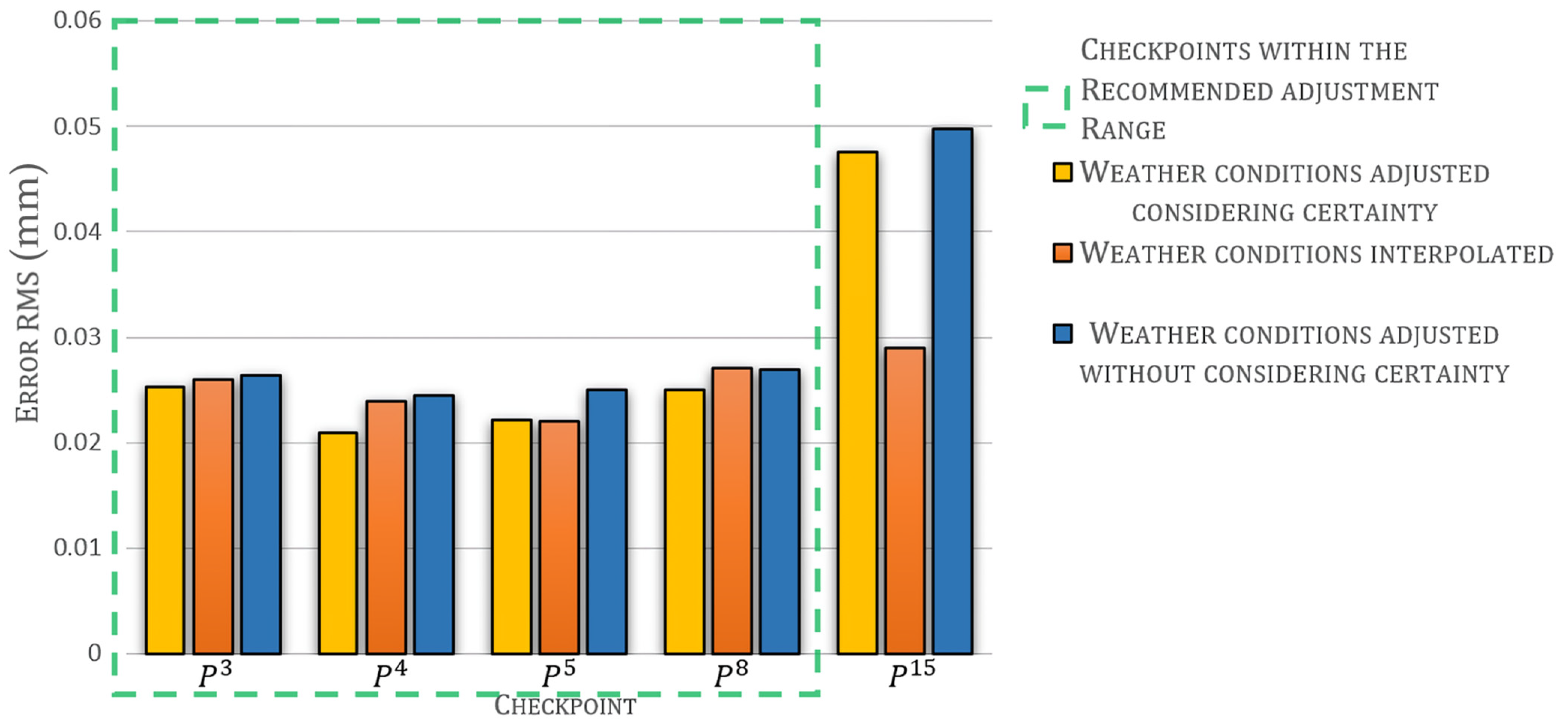
Moreover, Figure 10 depicts the performance of adjustments for $C{a}_{i=2}^r$ at checkpoints $P^3,P^4,P^5,P^8,$ and $P^{15}$ considering the weather conditions certainty ${\eta }_2$as well as the performance without considering ${\eta }_2$.

The performance of the interpolation method is also included, e.g., at checkpoint $P^8$, the error without certainty ${\eta }_2$ is $E_{RMS}=0.0269$, which is similar to the error obtained from the interpolation method ($E_{RMS}=0.0271$), whereas the error considering the certainty ${\eta }_2$ $(E_{RMS}=0.025$) is less than both.

Although the certainty of weather conditions replication can be improved further by enhancing the adjustment model, its performance is better than IDW when the certainty distribution function is used. The benefits of including the weather conditions certainty are more evident in the case of rain.

In Table 12, the solar radiation adjusted ${Ca}_3^4$ presents an $E_{RMS}=0.0135$; meanwhile, the solar radiation interpolated ${CI}_1^4$ has an $E_{RMS}=0.0130$. Both errors are remarkably alike because solar radiation denotes less dependency on weather conditions variability in a narrow region as expected for a future soil moisture regional estimation.

Table 13 contains the comparison of wind speed results. The error from ${Ca}_4^4$ is $E_{RMS}=0.0536,$ and the error from ${CI}_1^4$ is $E_{RMS}=0.0600$. In this case, the adjustment model performs better than IDW because of the spatial analysis of the region. Wind speed adjustment is highly complex due to its changing conditions and the presence of natural or non-natural barriers that block the wind. This is usually not considered with some interpolation models, which can affect the soil moisture point estimate.

The adjustment model performs a more detailed modeling of potential evapotranspiration ${Ca}_5^r$, as well as of rain ${Ca}_2^r$. These two weather conditions are the most significant for the point estimation model because ${Ca}_5^r$ denotes the amount of water that outflows from the soil, whereas ${Ca}_2^r$ determine the water that is provided to the soil. According to Table 14, the adjustment model results ${Ca}_5^4$ present an error $E_{RMS}=0.0301$; meanwhile, the interpolation results ${CI}_5^4$ present an error $E_{RMS}=0.0322$.

All these errors are acceptable for the second objective of the adjustment model, i.e., the weather conditions applied to the point estimation model. The existing differences between weather condition measurements (${Cm}_i^4$) and weather conditions adjusted (${Ca}_i^4$) do not compromise the accuracy of the soil moisture estimation. In fact, there are some uncertainties or instrumental errors in some tests, such as $A,E,F,G,H,K,L,O,P$ from Table 10. An $E_{RMS}=0$ can be considered because the deviation between the adjustment model result $C{a}_1^4$ and the weather condition measured $C{m}_1^4$ is lower than the accuracy of the integrated sensor suite shown, e.g., in test $A$ from Table 10, the deviation between $C{a}_1^4$ and $C{m}_1^4$ is: $C{m}_1^4-C{a}_1^4=11-10.61=0.39;$ meanwhile, the accuracy of the ISS for temperature is $\pm 0.5$.

Furthermore, despite similar results from the adjustment model and inverse distance weighing (IDW), or even better IDW results, such as for temperature $C{a}_1^4$ and solar radiation $C{a}_3^4$, the adjustment model presents two advantages over the spatial interpolation IDW for developing the application proposed in Section 2 of this paper. The first advantage is a better performance when adjusting an inconsistent variable such as rain. The weather conditions certainty ${\eta }_2$ is responsible for this result. The second is that the adjustment model does not require deploying more than one measuring station when it is operating, unlike interpolation methods, which need more than one measuring point to perform the interpolation.

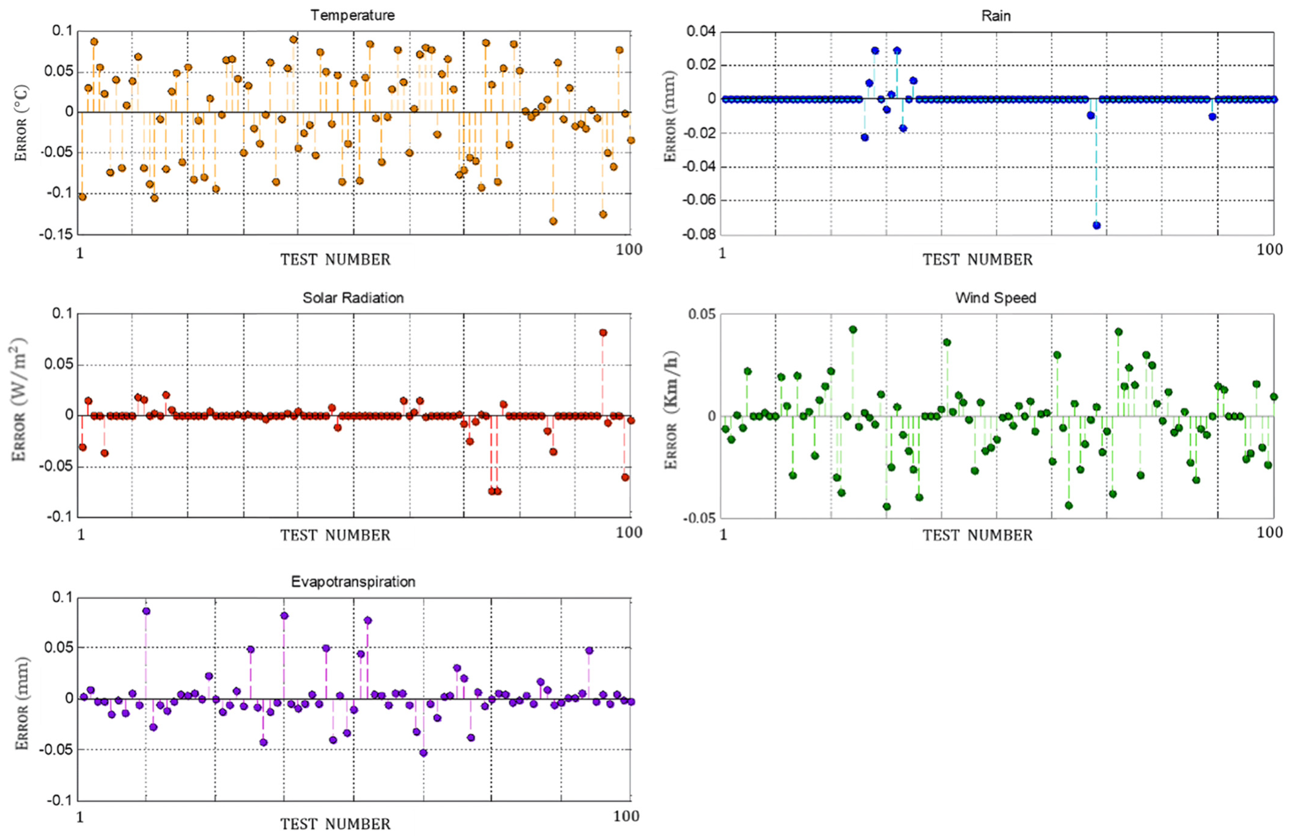
The adjustment model was also tested at other checkpoints, such as checkpoint $P^5$. Figure 11 depicts the error of weather conditions adjusted ${Ca}_i^{15}$ at checkpoint $P^{15}$. Checkpoint $P^{15}$ is located out of the recommended adjustment range. The distance from checkpoint $P^0$ and the different landscape features reverberate in the accuracy of the results. The normalized errors $E_{RMS}$ at checkpoint $P^{15}$ are the following:

• $E_{RMS}=0.0467$ for temperature.
• $E_{RMS}=0.0475$ for rain.
• $E_{RMS}=0.0187$ for solar radiation.
• $E_{RMS}=0.1182$ for wind speed.
• $E_{RMS}=0.0386$ for evapotranspiration.

Figure 11. Errors of weather conditions adjusted ${Ca}_i^{15}$ at checkpoint $P^{15}$.

Figure 11. Errors of weather conditions adjusted ${Ca}_i^{15}$ at checkpoint $P^{15}$.

In the case of ${Ca}_{i=\mathrm{1,3},5}^{15}$ (temperature, solar radiation, and evapotranspiration), the errors remain remarkably similar to those obtained at checkpoint $P^4$ due to the maximum increase in the errors is 0.0085. For ${Ca}_{i=2}^{15}$ (rain), the error increase is 0.0266. Both error increases show that the distance between the primary checkpoint influences weather condition adjustments $P^0$ and the checkpoint where the adjustment is performed $P^r$. The case of ${Ca}_4^{11}$ (wind speed) shows a remarkable increase of 0.0646 in the error. This error increase is caused not only by the distance issue but also by the changing wind behavior conditions in a region with a substantial amount of natural or non-natural barriers. Nevertheless, in farmland, it is not usual to find barriers scattered along the region of interest.

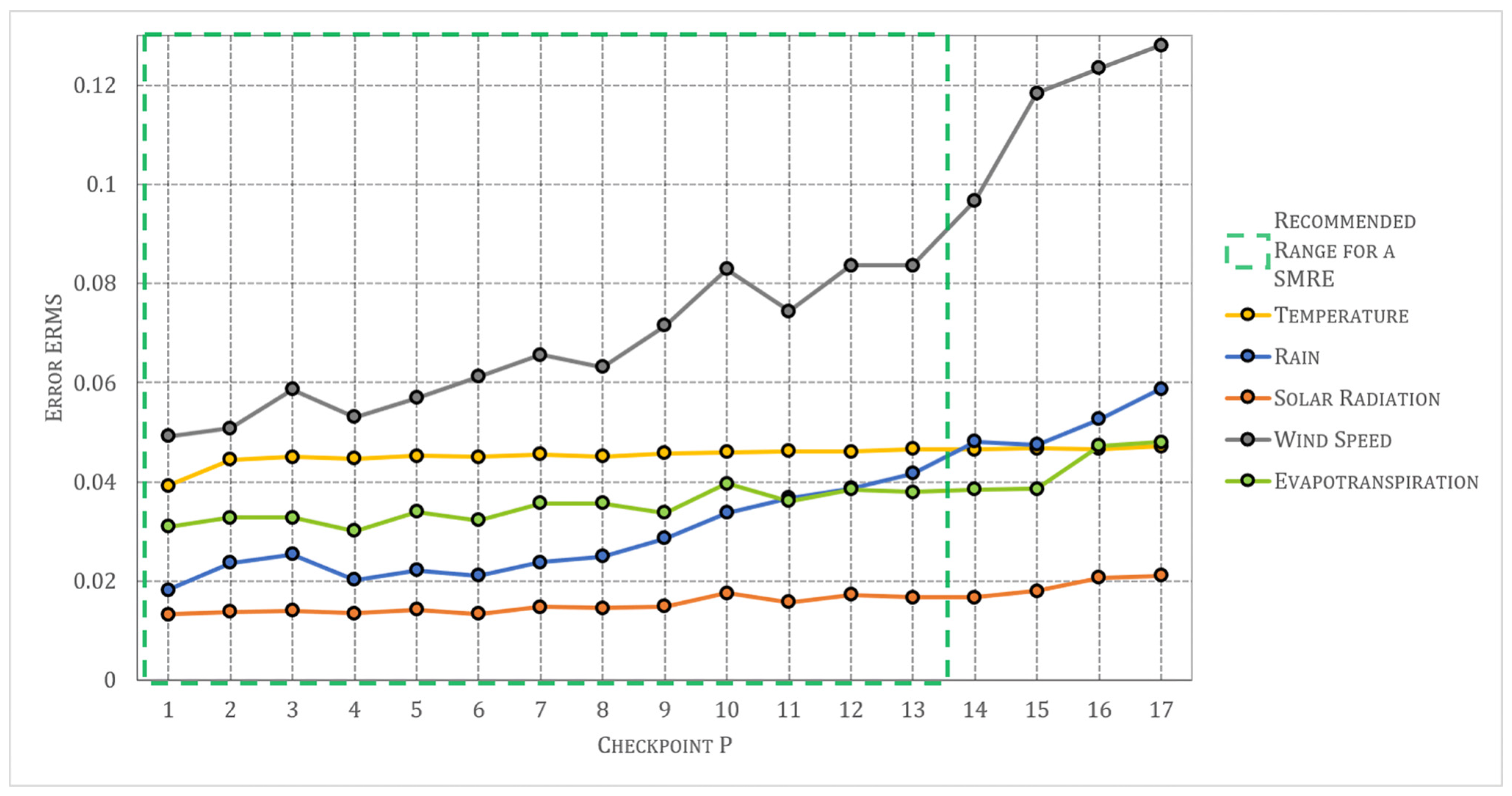
Figure 12 depicts the error $E_{RMS}$of the adjusted weather conditions compared with those measured at every checkpoint. In this paper, the recommended adjusting range of the adjustment model is 1.4 km, measured from $P^0$. Considering the location of checkpoints from Table A.1., the recommended adjusting range includes checkpoints $P^1$ to $P^{13}$. This range is defined based on the error of weather conditions adjusted. Not all weather conditions adjustments beyond this distance present a significant error. For example, the error of $C{a}_1^{15}$ (temperature) is $E_{RMS}=0.0447$ at checkpoint $P^{15}$ ($\cong 1.5$km from $P^0$); however, if a weather condition with an important error ($E_{RMS}\ge 0.1$) is supplied to the point estimation model, e.g., the error of $C{a}_4^{15}$ (wind speed) is $E_{RMS}=0.1182$ at checkpoint $P^{15}$, an erroneous point estimate could be obtained. The recommended adjusting range depends on the features of the region where the adjustment is performed. A more homogeneous region can increase the range. An adjustment region like the one presented in this paper can be considered a small-scale region. This kind of region presents limited variations in weather conditions but can strongly affect soil moisture. However, the adjustment model is intended to be part of a soil moisture regional estimation where an accurate modeling of the small variations in weather conditions is required.

The integrated suite sensor utilized by the adjustment model to measure at the primary checkpoint $P^0$ transmits the data to a console, which must be indoors; thus, the location of $P^0$ must be at least 300 m from this console, which is the transmitting range of the integrated sensor suite. Signal repeaters can be used if a more extensive transmitting range is needed. The transmission is made via radio frequency; the adjustment model needs no other connection (telephony or Internet). In addition, the primary checkpoint $P^0$ is recommended to be located at a centric sector $S\left(x,y\right)$, which accomplishes the condition abovementioned. A proper location of checkpoint $P^0$ directly affects the recommended adjusting range. In this paper, a set of $P^{r=1,\dots ,17}$ checkpoints is defined to validate the adjustment model; however, the aim is that any sector $s\left(x,y\right)$ can be a checkpoint when the adjustment model is implemented.

At 1.4 km from checkpoint $P^0$, the model is most effective for an intelligent adjustment of weather conditions based on spatial features; however, changes that will be highlighted in the following paragraphs can be made. Using only one integrated sensor suite in a range of 1.4 km, the almost null maintenance needed by the measurement devices and the non-use of measurement devices in situ throughout the region can help small farmlands reduce the complexity (physical and financial) of measuring soil moisture. Additionally, as the adjustment range is 1.4 km, a group of small farmlands can join to implement this method.

The appropriate size of the estimation region is related to the complexity of the ground conditions. The more heterogeneous the region is, the less precise the estimation is, which can be improved with the installation of another meteorological station that would create a new estimation region adjacent to the existing one, and it can even be carried out in the future by including remote sensing to increase the precision of the estimate and the extent of the region if required. However, this can be seen as the collaboration of two estimation regions. When the ground conditions change abruptly concerning those of checkpoint $P^0$, it is advisable to carry out the above. That is why it is essential to choose as a checkpoint a place representative of the terrain conditions that predominate in the study region.

The model can be complemented with remote measurements of meteorological variables. This would increase the estimate’s precision in the study region; however, it would also increase the operational complexity, i.e., the model would be more exposed to a failure or erroneous estimation if the remote measurement units break down or are vandalized. Remote sensing is recommended if the study region is complex enough (heterogeneity in terrain conditions), and it is necessary to improve the estimate’s precision and accept the increase in operational complexity.

During one year, our team verified that the integrated sensor suite ensures the reliable measurement of data of meteorological variables; likewise, other portable measurement devices were used for verification. However, unreliable data from the primary checkpoint $P^0$ could be due to heterogeneity in terrain conditions; in this case, it is advisable to evaluate if checkpoint $P^0$ is a place adequately representative of the terrain conditions that predominate in the study region. In addition, remote sensing or the collaboration of two adjacent estimation regions can be recommended.

5. Conclusions

The adjustment model developed herein aims to determine the weather conditions within a region to assist the point estimation for a regional estimation of soil moisture. In the adjustment model, the weather conditions are measured at a primary checkpoint; then, each one is adjusted according to the spatial features of each checkpoint. The adjustment of weather conditions avoids the implementation and maintenance of a measuring network.

The adjustment model can be easily implemented at any irrigation region that fulfils the stipulations; it is only required to introduce the new irrigation region’s satellite imagery, the checkpoint set’s location, and the soil and crop features. The initial parameters of the model can be refined as the approach collects more data while operating, which can be an advantage for small farmlands where there may be no previous data. Initial parameters must be reset if the irrigation region suffers a landscape alteration.

The results prove that the adjustment model presents a different performance for each weather condition adjusted. Solar radiation ($C{a}_3^r$) presents the best performance, whereas wind speed ($C{a}_4^r$) displays the worst performance. The performance depends on the modeling complexity of each weather condition. Unlike interpolation models, the model developed introduces the certainty of weather condition replication to improve the adjustment variables such as rain, whose behavior can be inconsistent within a region, e.g., the rain ($C{a}_2^4$) error derived from the adjustment is $E_{RMS}=0.0209,$ which is smaller than the error $E_{RMS}=0.0239$corresponding to rain ($C{I}_2^4$) derived from an interpolation method. Moreover, in some tests, uncertainties such as ISS accuracy do not allow for determining which approach performs better. The performance of the adjustment model is generally similar to or better than the performance of the interpolation method. However, the fuzzy approach utilized in this model does not require more than one measuring checkpoint, unlike interpolation methods, which do require that; this is an excellent advantage according to the aim of this paper. Overall, the results demonstrate that despite the existence of a negligible error, the weather condition adjustments avoid measuring them at every checkpoint within an adjusting range; in this case, 1.4 km from checkpoint $P^0$. As a result, the adjustment model of this paper and the previously published point estimation model would integrate an automatic regional estimation of soil moisture, which only requires the irrigation region data and a reduced number of measurements.