
Numerical Modeling of Water Jet Plunging in Molten Heavy Metal Pool

1
Ishlinsky Institute for Problems in Mechanics of the Russian Academy of Sciences, Moscow 119526, Russia
2
National Research University “Moscow Power Engineering Institute”, Moscow 111250, Russia
3
JSC “Electrogorsk Research and Development Center for NPP Safety”, Electrogorsk 142530, Russia
*
Author to whom correspondence should be addressed.
Mathematics 2024, 12(1), 12; https://doi.org/10.3390/math12010012
Submission received: 8 November 2023
/
Revised: 7 December 2023
/
Accepted: 18 December 2023
/
Published: 20 December 2023
(This article belongs to the Special Issue Numerical Simulations and Mathematical Modelling in Engineering Physics)
Abstract
:The hydrodynamic and thermal interaction of water with the high-temperature melt of a heavy metal was studied via the Volume-of-Fluid (VOF) method formulated for three immiscible phases (liquid melt, water, and water vapor), with account for phase changes. The VOF method relies on a first-principle description of phase interactions, including drag, heat transfer, and water evaporation, in contrast to multifluid models relying on empirical correlations. The verification of the VOF model implemented in OpenFOAM software was performed by solving one- and two-dimensional reference problems. Water jet penetration into a melt pool was first calculated in two-dimensional problem formulation, and the results were compared with analytical models and empirical correlations available, with emphasis on the effects of jet velocity and diameter. Three-dimensional simulations were performed in geometry, corresponding to known experiments performed in a narrow planar vessel with a semi-circular bottom. The VOF results obtained for water jet impact on molten heavy metal (lead–bismuth eutectic alloy at the temperature 820 K) are here presented for a water temperature of 298 K, jet diameter 6 mm, and jet velocity 6.2 m/s. Development of a cavity filled with a three-phase melt–water–vapor mixture is revealed, including its propagation down to the vessel bottom, with lateral displacement of melt, and subsequent detachment from the bottom due to gravitational settling of melt. The best agreement of predicted cavity depth, velocity, and aspect ratio with experiments (within 10%) was achieved at the stage of downward cavity propagation; at the later stages, the differences increased to about 30%. Adequacy of the numerical mesh containing about 5.6 million cells was demonstrated by comparing the penetration dynamics obtained on a sequence of meshes with the cell size ranging from 180 to 350 µm.
Keywords:
numerical simulation; VOF method; multiphase hydrodynamics; heat exchange; phase transition; nuclear safety; lead-cooled fast reactor; severe accident; water–melt interactionMSC:
76T06; 76T301. Introduction
Melt–water interactions can be featured by significant dynamic effects due to the rapid boil-up of volatile coolant upon contact with high-temperature molten material. Such events are encountered in nature (underwater volcano eruptions); however, they draw close attention in connection with hazards of industrial accidents in nuclear or smelting industries. Major research efforts were focused on the problem of steam explosions upon severe accidents with core meltdown in water-cooled nuclear power reactors. With the advent of heavy metal cooled-fast reactors, a relevant problem arises due to possible steam generator tube rupture (SGTR) accidents, when a high-pressure vapor–water mixture can flow into the space filled with lead melt at a much lower pressure [1]. Such an event can be dangerous due to jet impact on the adjacent tubes and structures, as well as heavy coolant oscillations in the steam generator. In order to understand the complex features of melt–water interactions and evaluate their consequences, experimental research and empirical studies must be accompanied by the development of theoretical approaches. Below, a brief overview of the existing knowledge in the field is presented, and the main knowledge gaps are identified.
Experimental studies on water interaction with molten pools of heavy metals have, for the most part, been related to the problem of steam generator tube rupture (SGTR). This event triggers several physical processes that, taken together, determine the impact on the internal structures of the steam generator, as well as on the reactor as a whole [2]. After the tube is damaged, the critical discharge of water is established almost instantly in the rupture, followed by the critical discharge of vapor–water mixture [3]. Therefore, the water flowrate through the rupture is determined solely by the high pressure in the heat exchange tube, being independent of the much lower pressure in the molten lead. Due to water discharge, a depressurization wave propagates upstream from the failure location towards the tube inlet connected to the collector providing feedwater to the heat exchange tubes of the steam generator. As a result, a much higher than nominal pressure drop will be established between the tube inlet and rupture point, with the water pressure near the rupture being determined by the critical discharge conditions. In the conditions of significant pressure decrease, water becomes superheated and boils up near the rupture, so that two-phase mixture is going to flow out of the rupture opening.
The first portion of water ejected from the ruptured tube into the low-pressure molten lead becomes superheated and boils up, with a sharp increase in the volume. This process generates the propagation of a shock wave in the molten lead. Since the expansion of the two-phase mixture in the molten lead is relatively slow due to the high density of the melt, the shock wave is of quite low amplitude, having no significant impact on the steam generator internal structures [4].
After the termination of fast wave processes, the discharge from the steam–water mixture reaches a quasi-steady state, and a multiphase mixture of molten lead, water, and steam is formed near the rupture’s opening. Steam is ejected out of the tube; additionally, it is generated by the evaporation of the released water due to (i) the rapid pressure drop to the level in the surrounding molten lead, making water superheated and causing its bulk boil-up; and (ii) contact with high-temperature surrounding lead.
Since the molten lead temperature exceeds, by far, the boiling temperature of water, direct contact between the water and melt is thermodynamically prohibited, and a vapor film separates the two fluids. In these conditions, heat transfer from melt to water proceeds in the film-boiling regime, with the convective flow of vapor in the film determining the heat exchange intensity. In the experimental work [5], a value of 145 W/m2 K was obtained for the heat exchange coefficient for the film boiling of water droplets with a diameter under 1 cm, surrounded by vapor film and rising in molten lead with the temperature of 500–600 °C. This value is about two orders of magnitude lower than in the case of direct water–melt contact. The relatively low heat transfer rate, limited by the film boiling, allows the quite long existence (about dozens of seconds) of the “melt–vapor–water” multiphase system.
The experimental studies on water jet interaction with molten lead–bismuth eutectic performed in a LIFUS5 facility are reported in [6,7]. In these experiments, 80 L of melt with the temperature of 400 °C was placed in the test vessel, and the gas space above the melt surface was filled with argon at a pressure of 0.1 MPa. Water was injected into the vessel under the melt level through a pipe with an internal diameter of 18 mm; the injection time was 3 s, water pressure was 18.5 MPa, and water temperature was 300 °C (subcooling of 59 °C). In the course of the experiment, pressure and temperature were measured at various vessel points.
The first (very sharp) pressure spike of the order of 3.4 MPa was registered at the instant of initial water discharge; it was related to fast expansion of water in the low-pressure melt. Then, the vessel pressure dropped to 0.3 MPa, after which, over the time of 0.5 s, it rose to 2.5 MPa or became 25 times higher than the initial vessel pressure. This pressure rise indicates that this period was featured by intensive water jet interaction with the melt. Afterwards, the vessel pressure decreased to about 1 MPa and stayed at that level until the termination of the water supply to the test vessel; finally, the pressure dropped to about 0.5 MPa.
A different experimental setup was used in [8,9,10], where the evolution of a water volume submerged in a melt pool was studied. The interaction proceeded in a cylindrical vessel with the internal diameter of 140 mm, filled with molten alloy of Bi 60%-Sn 20%-In 20%; the melt density was 8500 kg/m3, and the melting temperature was 79 °C. Water was delivered under the melt level in a fragile cone-shaped glass flask with a flat bottom. The contents of the flask were transported into the melt at the speed of 250 mm/s; it was ruptured by a crushing cone pre-positioned on the bottom of the interaction vessel. As a result, direct contact between the water and the surrounding melt occurred, initiating their interaction. In the course of the experiment, the pressure and temperature were measured by respective transducers installed at several points in the vessel. In the experiments, the water volume was in the range of 5–100 cm3, and its initial temperature was 58–99 °C. The initial melt temperature was in the range of 296–545 °C, and the initial pressure in the gas space above the melt was 0.1 MPa. After the flask rupture, the melt–water interaction was signified by the rise in the in-vessel pressure by approximately an order of magnitude. However, the peak pressure registered in these experiments was lower than in LIFUS 5 tests. A probable reason for this difference is that, when water is supplied into the melt vessel as a jet, the fragmentation of water and melt occurs, creating an intensive interaction between the materials. In the experiments [8,9,10], however, the water–metal contact occurs on the surface of the initial water volume, where fragmentation is quite moderate.
In 2018, experimental results on water–melt interaction were published [11], obtained on a facility closely resembling that used in References [8,9,10], with the following differences: (i) the internal diameter of the test vessel in [11] was 250 mm; (ii) the glass flask was spherical; (iii) its breaking was performed via contact with vessel bottom, without a crushing cone; and (iv) the flask was transported into the melt at a speed of 100 mm/s. The results obtained in [11] confirmed the conclusions of experiments [8,9,10]: in the conditions where the mixing of the materials was of low intensity (as opposed to water injection into melt as a jet), the interaction is featured by relatively low levels of pressure rise in the vessel.
Water jet interaction with lead–bismuth eutectic alloy (density, 10,600 kg/m3; melting temperature, 125 °C) in a flat vessel (slice geometry) was studied in the experiments [12,13,14]. The vessel was 150 mm high, its width was 170 mm, and its thickness was 10 mm. The bottom surface of the vessel was rounded. Subcooled water impacted the melt surface for 0.5 s; it was supplied through a vertical tube with and internal diameter of 6 mm. The outlet of the tube was located 50 mm above the initial melt surface, and the gas space was connected to the atmosphere. In the experiments, the initial water temperatures were 25, 60, 80, and 90 °C; and the melt temperatures were 273, 280, 290, 480, 500, and 530 °C. The water jet velocity varied in the range from 5.8 m/s to 7.8 m/s. Visualization of the melt and water phases was performed by high frame-rate neutron radiography. At the initial stage of the water–melt interaction, the formation and then expansion of a cavity filled with water and vapor were observed, signified by the boiling of water on the cavity’s surface. Later on, this interaction proceeded differently, depending on the water jet velocity and initial temperatures of the water and melt. In some cases, energetic interactions were observed, as indicated by a significant pressure increase in the melt, which even caused plastic deformations of the vessel walls manufactured from 1 mm thick stainless steel.
The above overview of experimental results clearly demonstrates the difficulties encountered by experimentalists: the interactions between the water jet and melt pool are of short duration, and the presence of opaque melt prevents the use of optical registration methods requiring application of a lot more sophisticated X-ray and neutron radiography techniques. Also, large-scale tests are expensive, while laboratory-scale results are difficult to scale to the dimensions required for the evaluation of reactor safety. For this reason, the development of analytical and numerical approaches to the simulation of fluid dynamics and thermal processes in water–heavy-metal interactions is of significant fundamental and applied value. In particular, detailed numerical simulations provide a possibility to fill the knowledge gaps on the processes that are not amenable to direct experimental measurement.
There exist two principal approaches to the mathematical modeling of the systems, and they are considered here. The first one (multifluid models) is based on the concept of multiphase fluid mechanics [3,15], where each phase (fluid) is described as a locally volume-averaged continuous field having its own volume fraction, velocity, and temperature. Several universal multiphase flow types (bubbly flow, dispersed droplet flow, etc.) correspond to some particular combinations of phase volume fractions and some other parameters (so-called flow regime maps). The phases interact via heat and mass exchanges, as well as drag; these interactions are described, as a rule, by empirical or semi-empirical correlations derived from a large volume of experimental data. A distinctive feature of this approach is that the interfaces between the phases are not resolved directly; rather, the volume-averaged specific interface area is taken into account in the correlations for interphase interactions.
One of the computational codes based on the multifluid approach is SIMMER-III [16], a code developed for the analysis of accidents in nuclear power reactors with liquid metal coolant. This code was applied in [7,17] to the analysis of the abovementioned LIFUS 5 experiments; also, it was applied in [16] to the analysis of experiments on the interaction of water volume submerged in a vessel with high-temperature melt [8,9]. Numerical simulations of these experiments by SIMMER-III demonstrated reasonable agreement with the test data in some cases, while significant differences were obtained in a number of cases. The principal problem in the modeling of a water jet injection in a melt pool is that there is a great variety of arising multiphase flow structures absent from the deterministic set of flow regimes implemented in the code. In such intermediate or transient cases, a description of the interphase exchanges is performed via interpolation between the flow regimes available in the code. Evidently, this can lead to the significant deviation of numerical results from the test data.
Another approach to the numerical modeling of multiphase flows is the direct numerical simulation where interfaces between the phases are tracked, and fluid dynamics equations are solved in each phase [18,19]. In contrast to the volume-averaged multifluid models, the phases are considered immiscible, transported by a common velocity; however, some velocity jumps can exist if phase change occurs on the interface. Quite a few interface tracking methods have been developed so far. These include the “sharp interface” immersed boundary (or level-set) method, where the interface is described as a geometrical surface corresponding to zero of the signed distance function; and the “smeared interface” method, where the interface is represented by a thin transitional zone. A popular interface tracking method of the latter type is the VOF (Volume-of-Fluid) method [20]. The volume fraction of each phase is a step-like function, changing abruptly from 0 to 1 at the phase interface. Numerically, however, this step-like behavior is approximated by a continuous function, allowing for some (controlled) phase mixing in the finite-thickness transitional layers representing the interfaces. As a result, simulations are performed for a single effective fluid with properties defined as volume fraction-weighted respective phase properties. Also worth noting are such interface tracking techniques as the phase-field model that was successfully applied to solidification problems, or the Lattice Boltzmann Method (LBM), which is based on the solution of kinetic equations (see review in [18]).
The VOF method gained its popularity in simulations of complex multiphase flows due to its relative simplicity and ability to naturally describe such complex processes as fluid fragmentation, the breakup and coalescence of jets, drops, etc. In reaction to the problem of melt–water interactions, VOF simulations of melt jet breakup in water were performed in the two-phase framework (no vapor phase present) in [21,22,23,24]. In particular, the VOF method was applied to numerical simulations of the interaction of a water jet issuing in a vessel filled with liquid lead [24]. In this work, mostly the fluid-dynamical aspects of the interaction were considered with no vapor taken into account. It was shown that, due to high density of the molten lead, the water jet rapidly loses its momentum and undergoes significant fragmentation. Size distribution function was obtained for the dispersed water fragments by processing the simulation results; it was shown that, for the assumed jet parameters (inlet velocity, 20 m/s; diameter, 12 mm), the highest fraction (by mass) has the average size of 4.5 mm.
In the current work, Reference [24] is extended in several important avenues. A complete three-phase system (melt, water, and vapor) is considered, with phase change on the water–vapor interface taken into account. Three-dimensional simulations are performed, allowing for a more adequate description of phase surface instabilities, fragmentation, etc., and then the two-dimensional simulations [24]. The VOF model’s capability of capturing the important features of melt–water interactions was validated in recent works [25,26], where single-droplet steam explosions, as well as melt splashes due to the impact of short-duration water jet on a shallow melt layer, were simulated.
Here, the model [25,26] was applied to a water jet’s interaction with a molten pool of heavy metal. Three-dimensional simulations were performed for the conditions of previous experiments [12,13,14], where a water jet was injected in a planar vessel filled with lead–bismuth eutectic alloy; the results obtained are compared with the experimental data.
Note that only a few attempts of two- and three-dimensional modeling of water–heavy-melt interactions, with account for the presence of three phases and phase changes, have been performed so far. For example, simulations of experiments [12] were performed on the basis of multifluid (volume-averaged) models in [27] (by MC3D code) and [28] (by two-dimensional ACENA code). The only VOF simulations known to the authors so far were performed in [29]; however, these simulations were performed for high-velocity water jets and in a different geometry. Therefore, the novelty of the presented research is related to the detailed three-phase modeling of water–melt interactions on the basis of the VOF model, formulated for compressible phase with evaporation on the interface, as well as in the validation of the predictions by this model against the experiments [12].
2. Statement of the Problem
The evolution of melt, water, and vapor separated by the respective interfaces is described in the framework of the Volume-of-Fluid (VOF) approach [18,19,20]. According to the VOF model for the total of phases, each -th phase is assigned a respective volume fraction, (such that ), and sharp interfaces are smoothed into thin zones where the volume fractions are continuous but change rapidly from 0 to 1. This interface smoothing allows one to solve the transport equations for the volume fractions on the Eulerian mesh without the need to track the interfaces as geometric surfaces, thus avoiding the problems of surface topology changes due to liquid fragmentation and coalescence, etc. The smoothed surface, however, requires the application of specific models to take into account the processes that proceed on the phase interfaces, including the effects of surface tension (related to the surface curvature) and phase changes. Typically, the surface processes are recast as equivalent volumetric source terms acting in the thin zone of high gradients of volume fractions, providing the same integrated quantities as their surface-related counterparts.
In this work, we applied the formulation of the VOF method that takes into account the phase compressibility (i.e., variation in the phase density, , with temperature and pressure), as well as possible phase changes on the interfaces. In the presence of phases, the phase continuity, momentum, and energy equations take the form of
where is the time, is the i-th phase density; is the volumetric source term describing the i-th phase appearance in phase transitions; , , and are the velocity, pressure, and temperature fields common to all the phases; and is the gravity acceleration. The viscous stress tensor in the momentum equation is written as
The momentum and energy Equations (2) and (3), as well as relationship (4), involve the volume fraction-averaged density, ; specific enthalpy, ; dynamic viscosity, ; and thermal conductivity, , defined by
In (5), the respective phase properties are determined from the respective equations of state and relationships for the transport coefficients:
where is the specific internal energy of the i-th phase. The surface tension force acting on the interfaces is , where the respective forces acting on each liquid phase interface are described by the continuous surface force (CSF) model [19]:
where is the surface tension of i-th fluid at the interface with vapor, and is the surface curvature of -th phase interface.
The last term on the right-hand side of energy Equation (3) takes into account heat release or consumption in the phase transition occurring between all physically possible phases. In the current work, however, we consider three phases (, including melt, water, and vapor, which are denoted hereafter by the subscripts , , and , respectively). In this system, phase transition can occur only on the water–vapor interface the water evaporation rate per unit volume is denoted by (with ), and is the specific heat of evaporation. Similar to the surface tension force (see (7)), the evaporation rate, , must be expressed as a volumetric source term distributed over the thin zone to which the interface is smeared in the VOF model (bulk boiling of water is not possible in this approach). Here, we use the evaporation model proposed in [30] (with slight modifications [25]), containing no user-defined constants:
where is the cell size, is the saturation temperature corresponding to the local pressure, and is the thermal conductivity of water. In the multidimensional problems where the mesh cells can have different sizes in different directions, the mesh cell size, , entering Equation (8) must be defined. The model (8) was derived in [30] from the comparison of water superheat energy (expressed by the temperature difference factor) and the conductive heat flux proportional to water conductivity divided by the distance between the current and adjacent cell centers. In the current implementation (see also [25]), all neighbors of the cell where phase transition occurs were checked, and the one having the highest water volume fraction was chosen for the determination of .
All of the gas phase is considered water vapor, with condensation suppressed; this allows us to simplify the model by avoiding the consideration of the multicomponent gas mixture, which does not play any significant role in the current problems where small amounts of water interact with high-temperature melt. In these conditions, water vapor rapidly becomes superheated upon contact with the melt, and its condensation is not possible, at least in the interaction zone.
Note finally that, unlike the classical VOF formulations, the current VOF model takes into account the effects of phase compressibility and phase changes. This can be demonstrated by recasting the phase continuity Equation (1) in the following form:
where is the material derivative. By summing up Equation (9) over all phases, it can be determined that the velocity field is subject to the constraint
with the first term on the right-hand side related to the compressibility of all phases; the second one describes dilatation due to vapor release and expansion.
3. Numerical Implementation and Verification
Numerical simulations were carried with the open-source CFD toolbox OpenFOAM-v2112 [31]. OpenFOAM (standing for Open-Source Field Operation and Manipulation) is an open-source toolbox containing a set of libraries that implement a wide range of operations (e.g., vector and tensor algebra operations, mesh function interpolation, integration, approximation of differential operators, linear algebra solvers, etc.). The libraries can be used to create executables implementing numerical solvers for a plethora of specific problems in continuum mechanics; the current distribution of OpenFOAM comes with a set of ready-to-use solvers, while new solvers and utilities can be created by users by writing respective main program and functions and relying on the methods implemented in the libraries to solve the resulting equations.
A new solver, fciFOAM, that allows one to model the flows of immiscible compressible phases separated by interfaces tracked by the VOF method with phase changes was developed; no standard solvers in OpenFOAM take into account both effects described by Equation (10). Pressure–velocity coupling in transient simulations is performed by using the familiar PISO method. The solver was verified on a set of test cases, including the one-dimensional Stefan problem and two-dimensional film boiling on a flat horizontal plate.
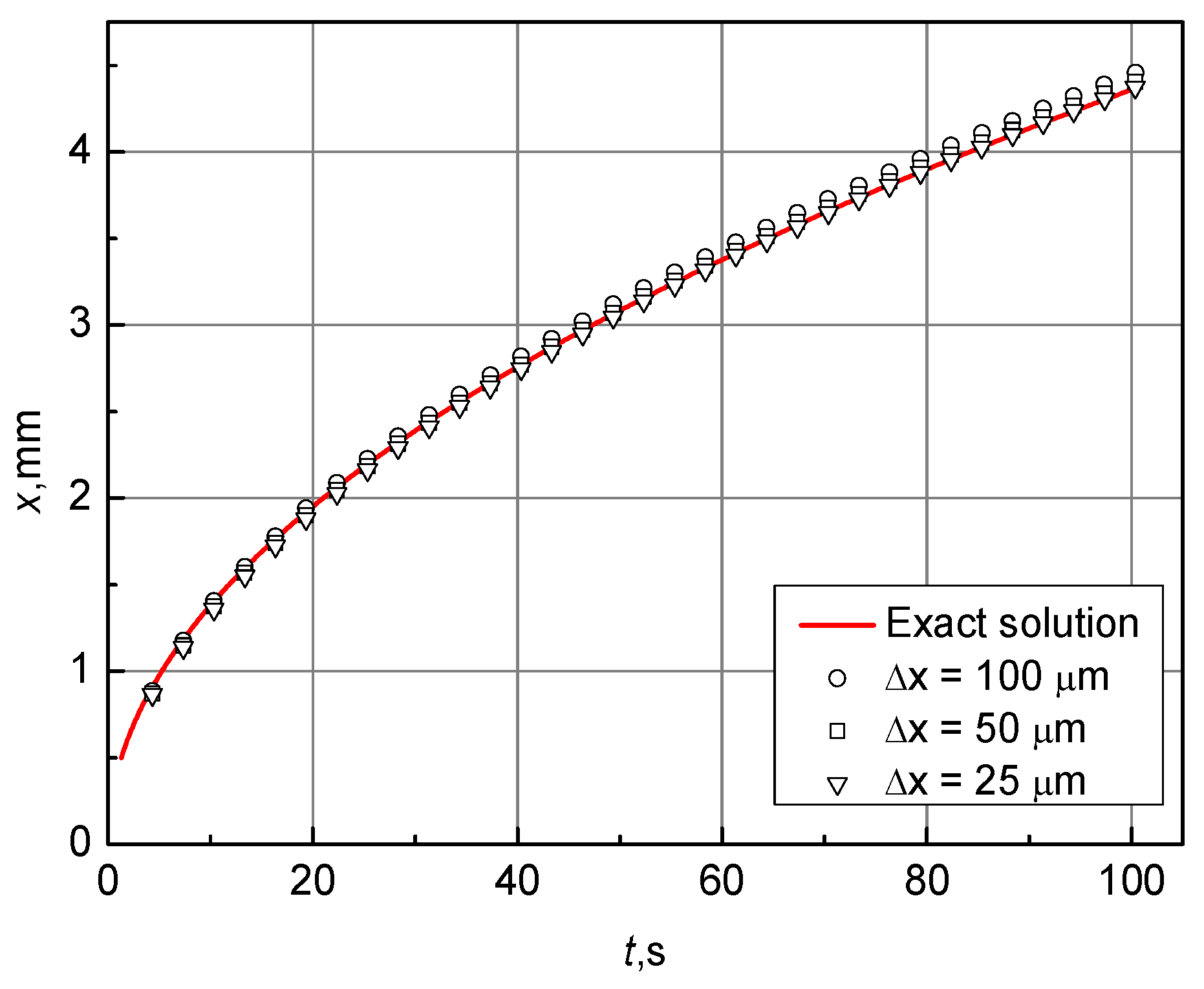
The 1D Stefan problem is a standard test in OpenFOAM for the verification of solvers with phase transitions. It considers the propagation of an evaporation front in a saturated liquid contacting a hot wall superheated with respect to the saturation temperature of the liquid. An analytical solution is available for the Stefan problem [32,33], making it a convenient problem for the verification of numerical solvers.
Simulations were performed for the following problem parameters: saturated water at the temperature of K is heated by a wall that is hotter by K, the water and vapor densities are kg/m3 and kg/m3, the corresponding specific heat capacities are J/(kg·K) and J/(kg·K), the thermal conductivities are W/(m·K) and W/(m·K), and the latent heat of evaporation is MJ/kg.
In Figure 1, the boiling front coordinate is plotted against time. The solid line represents the analytical solution; the dots correspond to the numerical simulations performed by fciFOAM on three different meshes, with the cell size, , indicated in the graph legend. It can be seen that the numerical results obtained on the mesh sequence converge to the exact analytical solution [32,33].
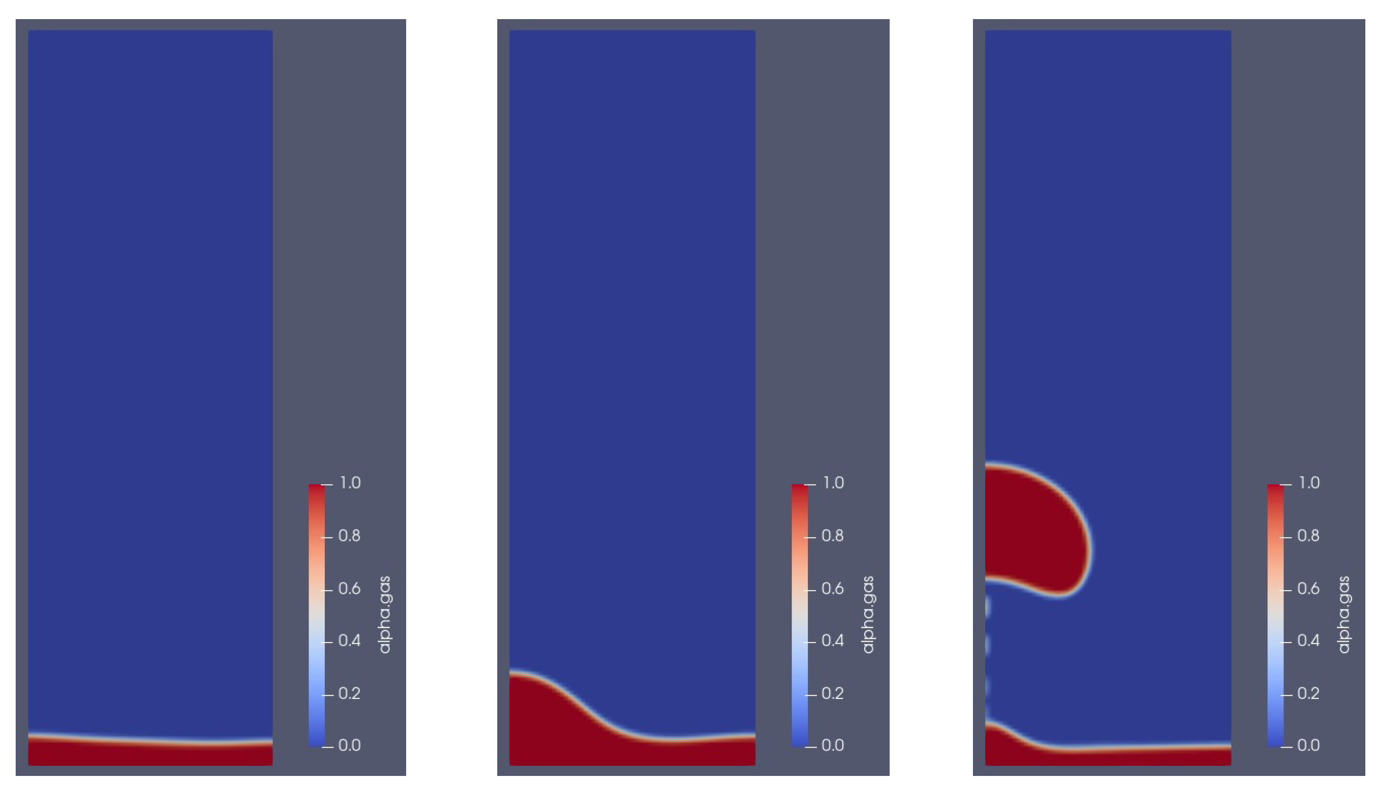
The second verification problem is the two-dimensional film boiling on a hot horizontal plate (see Figure 2). This problem was used for the verification of evaporation models in many works, particularly in [30,33]. Here, simulations were performed for the same model parameters as in [33]: the space above a horizontal wall is filled with saturated liquid at K, the temperature difference between the wall and liquid is K, and the corresponding liquid and vapor properties are as follows: densities, kg/m3 and kg/m3; dynamic viscosities, Pa·s and Pa·s; specific heat capacities, J/(kg·K) and J/(kg·K); thermal conductivities, W/(m·K) and W/(m·K); latent heat of evaporation, kJ/kg; and surface tension, N/m.
Initially, the hot bottom wall is separated from the liquid above it by a vapor film, with the thickness, , described as a function of the horizontal coordinate, :
where is the width of the film, equal to the “most dangerous” Taylor wavelength [34]:
where is the gravity acceleration.
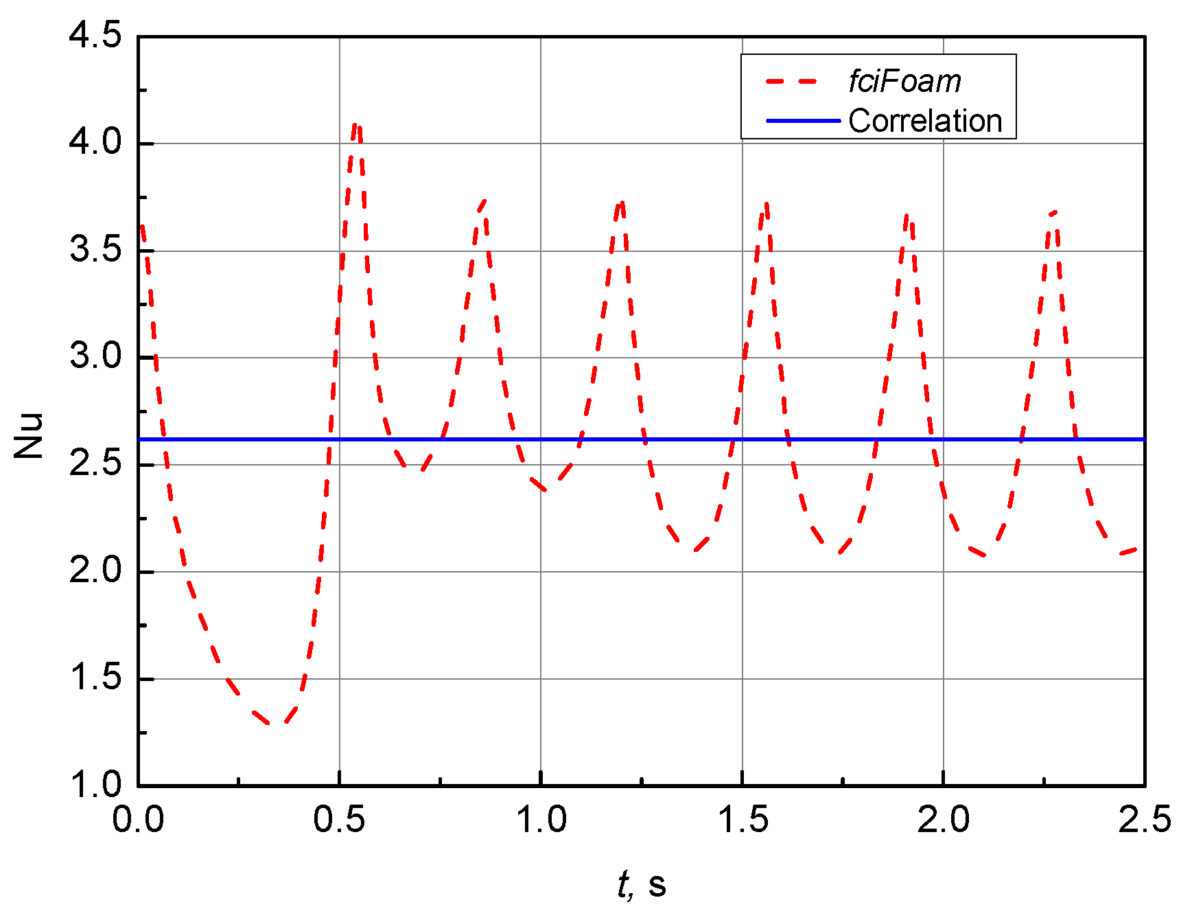
Periodic growth of mushroom-shaped vapor bubbles develops with time, leading to oscillations in the heat flux on the bottom plate. The space-averaged Nusselt number on the bottom wall (directed along the axis) is calculated by integrating the local Nusselt number defined by
where is a characteristic length
Then, the average Nusselt number is
In the simulations, the width of the bottom plate was taken to be .
In Figure 3, the time history of the average Nusselt number is presented, demonstrating that, following the initial few cycles, the process becomes periodic (after approximately 1.2 s), when the bubble detachment is followed by the formation of the subsequent bubble, repeating with the period of about 0.4 s.
The time-averaged Nusselt number can be obtained by averaging the Nusselt number (15) over a few periods at the stage where oscillations become periodic (see the last three oscillations in Figure 3). In the current simulations, the time-averaged Nusselt number obtained was equal to 2.56, which agrees quite well with the analytical solution [34] shown in Figure 3 by the solid line (the deviation is within 2.5%). This agreement is quite good, considering that, in other similar numerical works, the discrepancy in the Nusselt numbers reached some 30%.
The results obtained confirm that the developed solver fciFOAM is suitable for the solution of problems involving the interaction of the high-temperature melt with water, the key feature of which is the formation of large volumes of steam when the water boils. More validation results for fciFOAM obtained in different types of melt–water interactions can be found in [25,26].
4. Geometry and Parameters
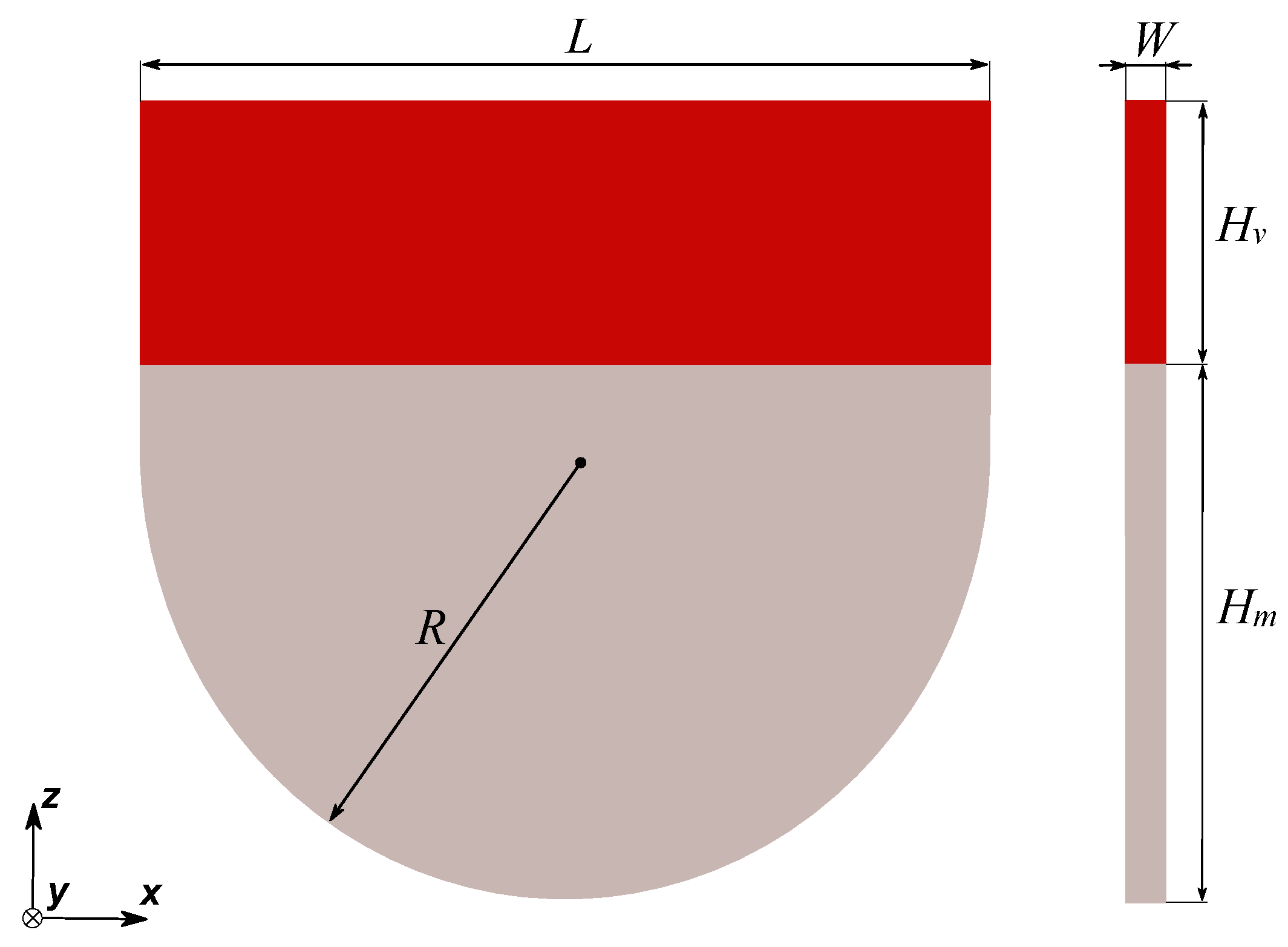
Simulations were performed in a computational domain reproducing the test section in experiments by Sibamoto et al. [12]. The upper part of the computational domain (see Figure 4) of the height mm represents the space filled with saturated vapor, while the lower part is a pool of hot melt with the depth of mm. The total width of the calculation domain is mm, and the radius of the bottom is mm. The upper boundary of the domain is open, with a round area of the diameter = 6 mm representing the subcooled water inlet. The remaining boundaries are adiabatic solid walls.
Numerical modeling was performed for the experimental case Run 4 [12] with the following parameters: jet velocity, m/s; melt temperature, K; and water jet temperature, 298 K. On the open upper boundary of the computational domain, a constant atmospheric pressure of MPa was maintained.
The melt pool material is lead–bismuth eutectic alloy with the physical properties taken from [35]; its properties are presented in Table 1, along with the properties of other phases (water and vapor). In the current problem, density changes in the water and melt are negligible in comparison with the compressibility of vapor; therefore, an incompressible liquid model was used for the liquid phases, while the ideal gas law was applied to vapor. Surface tension was set for each pair of phases: the surface tension on the water–vapor interface was N/m; on melt–vapor and melt–water interfaces, it was N/m.
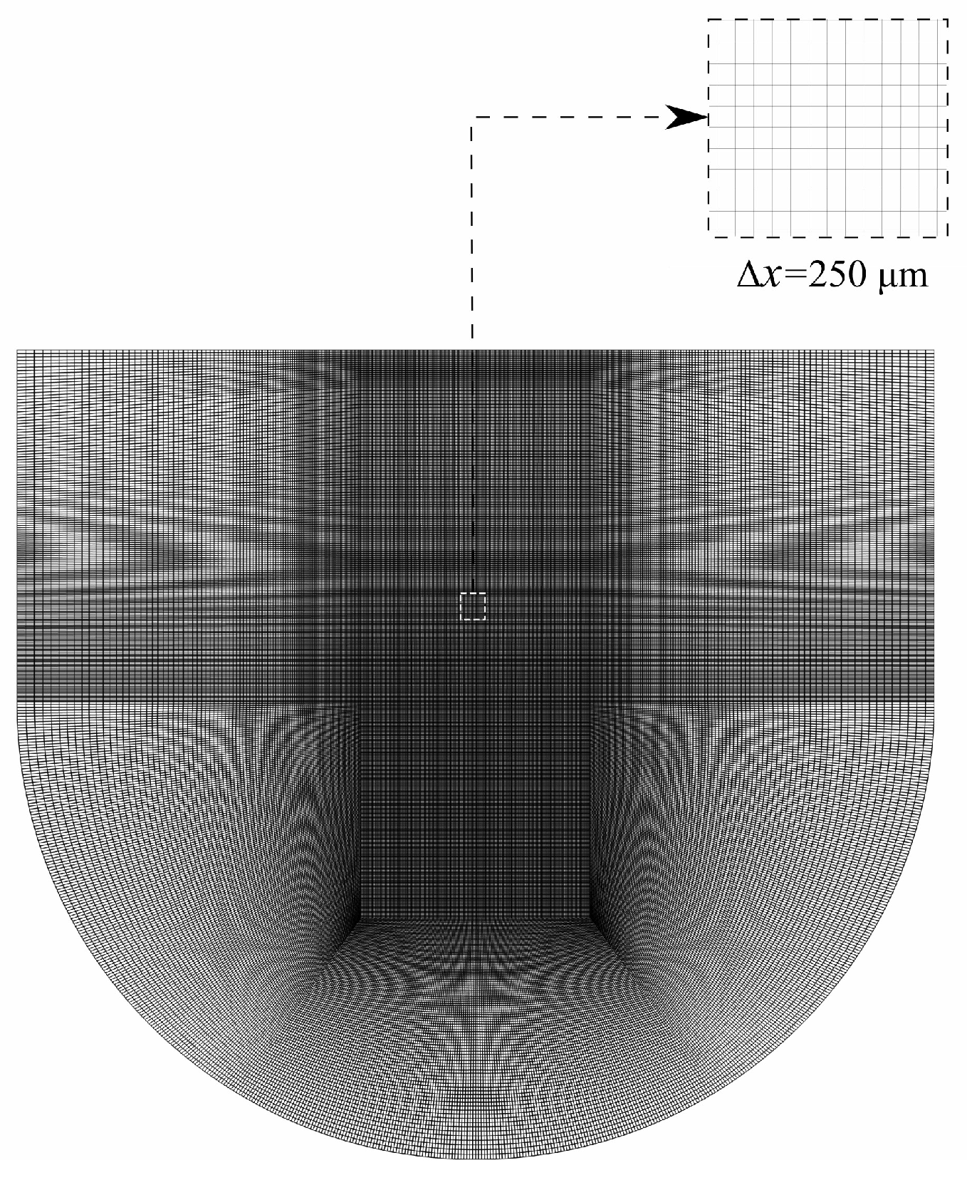
Simulations were performed on a multiblock structured mesh with 5,623,200 cells shown in Figure 5. The mesh was refined in the domain where the most important interactions (water jet fragmentation and cavity development) occurred; this domain was filled with cubic cells with a side length of µm. The required mesh size was determined in a set of preliminary simulations. We started our studies from coarse meshes (below 1 million cells), and it was found that, on such meshes, water jet fragmentation occurs very weakly, so that a nearly cylindrical water jet reached the vessel bottom, while the jet perturbations clearly seen in the experiments by Sibamoto et al. [12] were not reproduced at all. Gradual mesh refinement allowed us to obtain more realistic water jet fragmentation, and the qualitative picture obtained with the mesh containing 5,623,200 cells was found to be adequate. A simulation on an even finer mesh, with doubled cell count, was made afterwards in order to confirm that our “baseline” mesh was adequate, as a reasonable trade-off between the prediction accuracy and computational overheads. More details on the mesh sensitivity study can be found below, in Section 8 of the present paper.
5. Two-Dimensional Simulations of Nonboiling Water Jet Penetration into Melt
To better understand the three-dimensional effects and influence of water boiling on the interaction between water jet and a melt pool, a two-dimensional analysis of this process in the absence of water boiling was first performed. A set of two-dimensional calculations was carried out for water jet penetration into a molten-lead–bismuth alloy (the melt–water density ratio is ). The calculated results were compared with the results of simplified theoretical estimates [12] for the depth of the penetration of the water jet into the melt, , carried out for the case of the absence of water boiling.
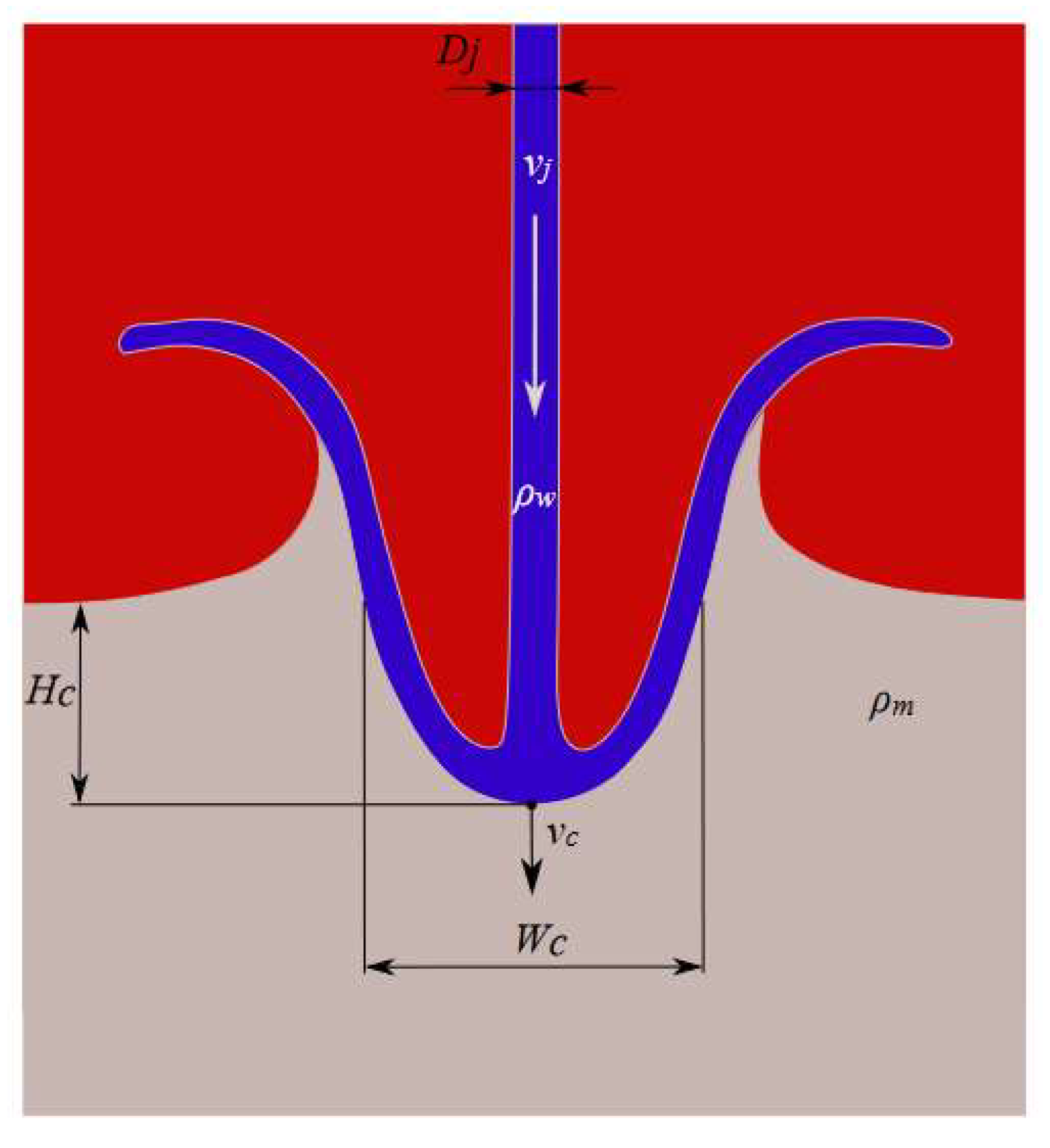
In Figure 6, the spatial distributions of phase volume fractions are presented for the case where a water jet velocity is m/s, and its diameter (width) is mm. Figure 6 is adapted from the actual simulation results at the instant ms, with the key geometric parameters added: is the depth of the jet penetration, is the width of the cavity formed in the heavy melt, and is the velocity of cavity propagation in the melt.
An estimate for the maximum possible steady-state penetration of a nonboiling jet was obtained in [12] from the balance between the jet stagnation pressure and the pool static pressure at the interface elevation:
where is the density ratio (for the molten-lead–bismuth alloy, to ), and is the densimetric Froude number. In fact, Equation (16) follows from the Bernoulli equation for the water jet; it predicts the quadratic dependence of the penetration depth on the jet velocity.
The water jet penetration in boiling liquids of different densities, ranging from 0.81 to 13.6, was studied experimentally in [36,37]. It was found that the jet penetration length (or the maximum cavity depth, ) is described by the linear function of the Froude number, , and, therefore, it depends linearly on the jet velocity, . In particular, the following correlation was obtained in [36]:
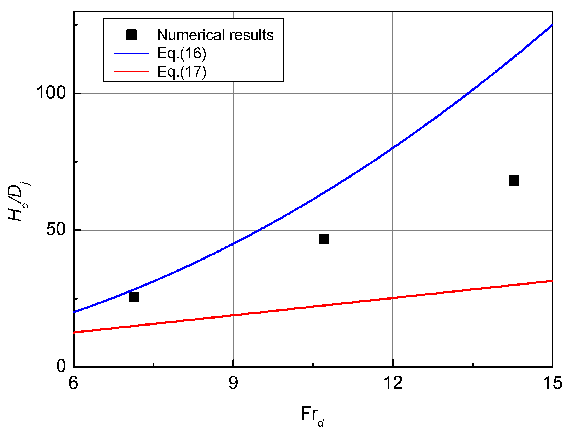
The influence of the jet velocity on the maximum depth of the jet penetration was studied in the set of two-dimensional simulations performed under the assumption of a nonboiling jet. The results obtained from the simulations (see Table 2) are compared with those predicted by Equations (16) and (17) in Figure 7. It can be seen that the predicted dependence of cavity depth on the densimetric Froude number is not quadratic, it is closer to the linear one. Evidently, this may result from neglecting the melt flow and drag forces in the estimate (16), while these factors are present in the experiments [36,37] and are taken into account in the current simulations.
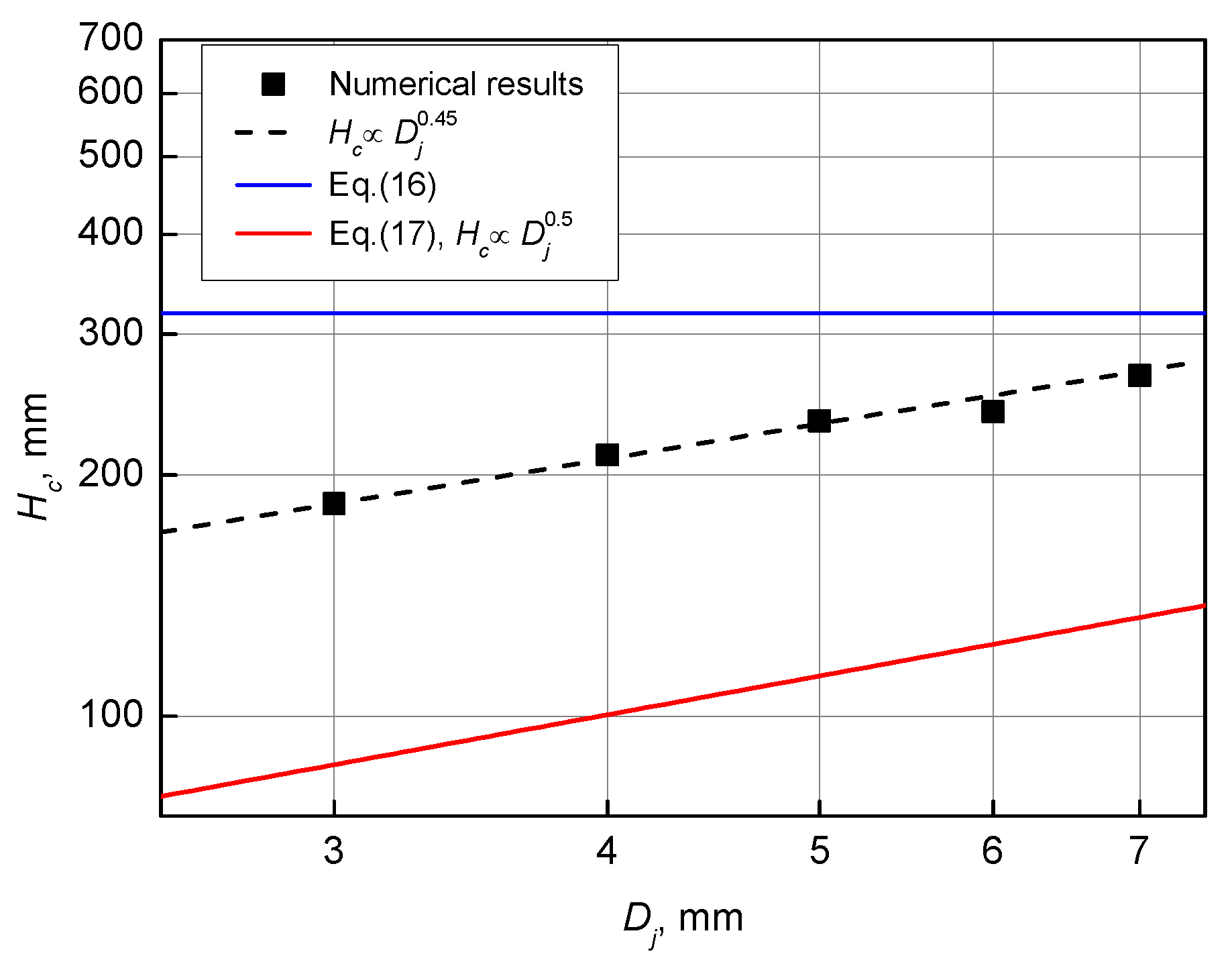
It is interesting to note that Equation (16) predicts that the maximum cavity depth, , is independent of the water jet diameter, , while Equation (17), which is based on the experiments of [36,37], predicts that . In order to check which conclusion is better reproduced numerically, a set of simulations was carried out where water jets of variable diameters were considered at a fixed jet velocity, m/s; the corresponding results are presented in Figure 8. It can be seen that our results confirm that the maximum cavity depth depends on the jet diameter; the calculated data are approximated quite well by the dependence , with the power index quite close to that in Equation (17).
6. Three-Dimensional Simulation of Subcooled Water Jet Penetration into Melt (Boiling Case)
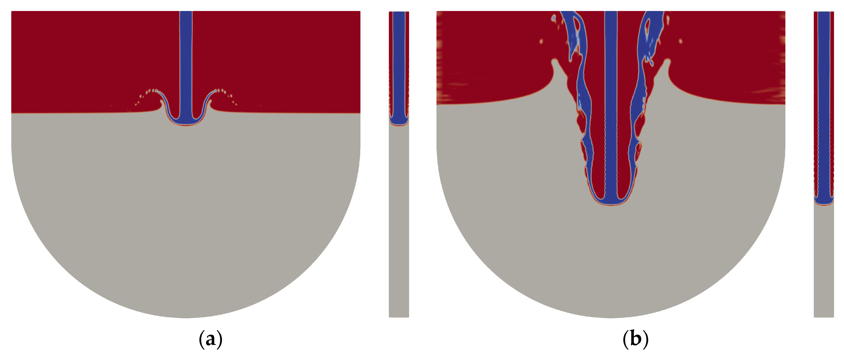
Consider now the 3D simulation performed in the complete statement of the problem, i.e., taking into account the phases changes. The simulation was carried out with the geometry and conditions corresponding to the experiment of [12], Run 4. Figure 9a–f present the evolution of the water jet in the melt pool: the volume fractions are shown for the melt (gray color), water (blue color), and vapor (red color) in the longitudinal and transverse planes of symmetry. The time instants are shown in the non-dimensional form, according to [12]:
The initial water jet penetration into the melt (see Figure 9a; ) was very similar to that observed in the 2D nonboiling case (see Figure 6). Water jet impingement on the melt pool surface leads to the formation and downward propagation of a cavity in the melt, filled with water and vapor. Simultaneously, a thin water layer spreads along the cavity’s surface. While in the 2D nonboiling case, the water layer thickness is almost constant over the cavity surface, in the boiling case, the water layer is thinner near the cavity bottom due to the evaporation and interaction with the generated vapor. At the instants , , and (Figure 9a–c), a thin vapor film separating the water from the melt is clearly seen. The vapor flow in this film provides heat transfer from the melt to the water (the film-boiling regime).
Figure 9c,d show that, as the water jets penetrates into the melt, pinching off begins in the middle of the cavity, with a two-phase vapor–water counterflow in the “neck”. Afterwards, breakup of the cavity into two parts occurs.
The subsequent stages of the process are illustrated in Figure 9e,f. Cavity formation due to water jet impact causes respective displacement of the melt in the shape of a “crown” around the cavity. After the maximum cavity depth is reached, the gravitational settling of the heavy melt begins, with a collapse of the lower cavity part and raising of the cavity with respect to the bottom of the vessel. This stage is characterized by unstable water boiling (see Figure 9e, ), significant deformation of melt surface, and breakup of water jet. With time, the surface area where heat transfer occurs increases, leading to the intensification of water boiling and vapor generation. The rising vapor captures some fraction of water, displacing it into the upper-cavity part. Due to these processes, the cavity assumes its quasi-steady shape (see Figure 9f, ).
In the subsequent experimental work [14], four stages of interaction were singled out by the analysis of radiographic images. All of these stages agree quite well with the current numerical simulation results: (1) water entry with gas entrainment (corresponds to in Figure 9a), (2) radial collapse of cavity (, Figure 9c), (3) breakup of water in cavity (, Figure 9d), and (4) boiling with unstable deformation of melt surface (, Figure 9f).
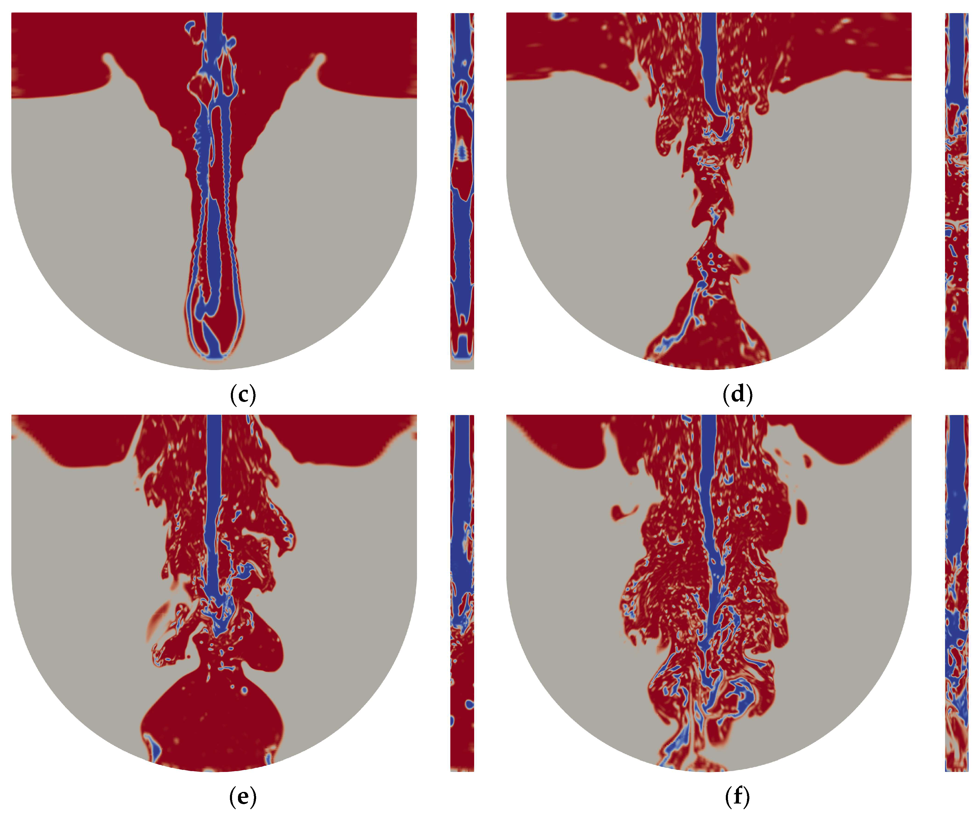
An insight into the melt–water–vapor mixing process can be achieved by inspecting the instantaneous shapes of water and melt surfaces. In Figure 10a–d, instantaneous shapes of water and melt surfaces (plotted as the level sets of the respective volume fractions, and ) are presented, further illustrating the process of melt–water interaction analyzed above. Such three-dimensional images are handy for better understanding the complex shape of the phase surfaces developing during the interaction, supplementing the phase volume fraction distributions in the cross-sections presented in Figure 9. It can be seen that, following the beginning of unstable boiling and collapse of the lower part of the cavity, not only the melt surface becomes very tortuous and random, but also some fine melt droplets are formed, also contributing to the phase mixing. The water jet becomes unstable and highly fragmented, with small droplets and irregular fragments being abundant in the whole cavity.
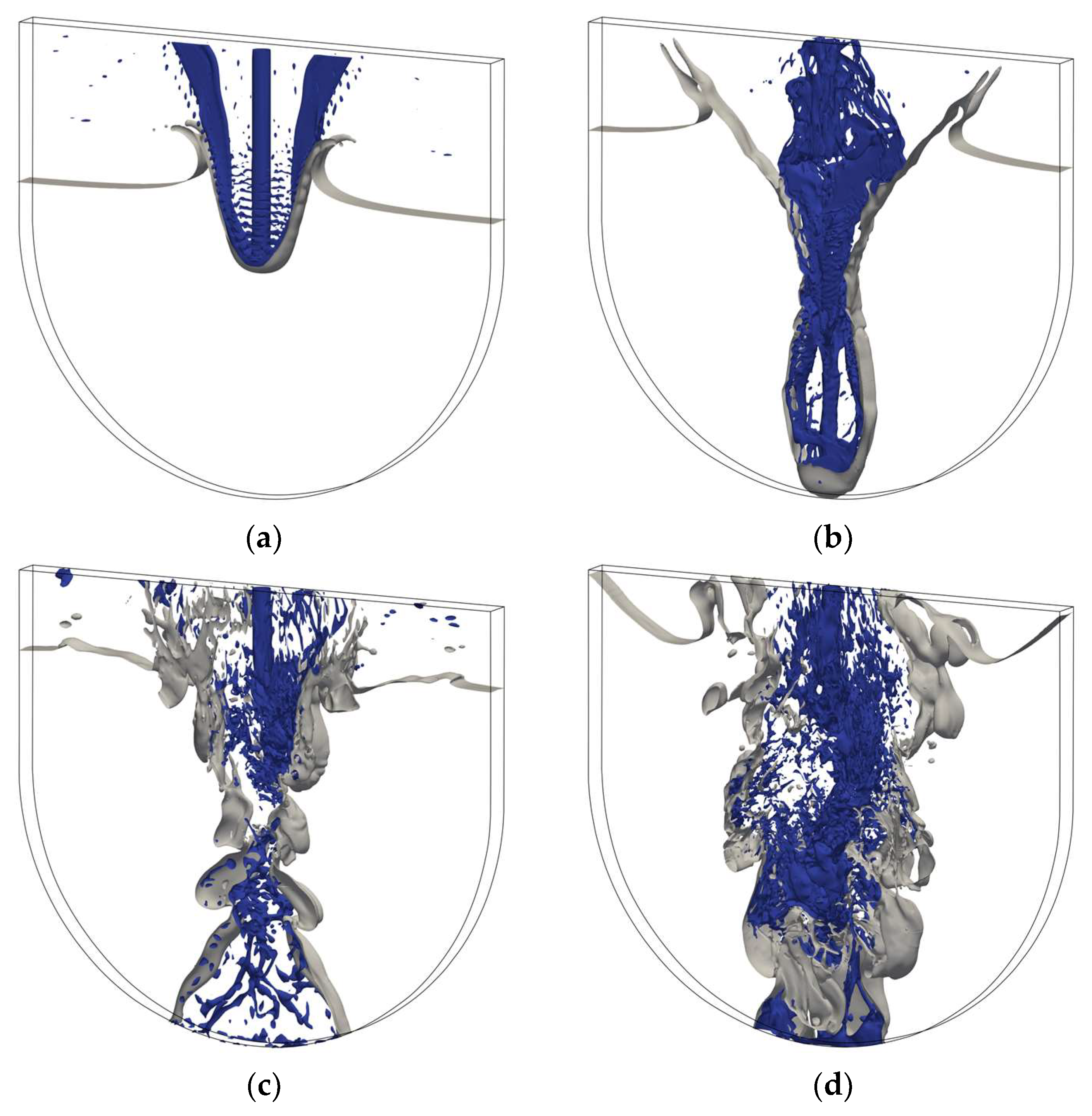
The dynamics of water jet penetration into the melt pool can be better understood by the analysis of the arising pressure field. For the simulation case, the pressure distributions at the same instants as in Figure 9 are shown in Figure 11.
It can be clearly seen that a zone of increased pressure is formed in the zone where the water jet is decelerated due to its contact with heavy high-inertia melt. This increased pressure turns water sideways and upwards, leading to the formation of bowl-shaped water flow (Figure 11a,b). The maximum pressure in this area, , depends on the water injection velocity; it is described by the Bernoulli equation, . For the parameters of the current simulation case, MPa, which agrees well with the maximum pressure levels in Figure 11a,b.
At the time (Figure 11c), the zone of increased pressure embraces the whole cavity. The melt contacting the cavity begins to flow, and the pressure drop in it decreases. The instant when the lower part of the cavity detaches (, Figure 11d) is characterized by increased pressure in the lower part of the cavity.
7. Comparison with Experiments [12]
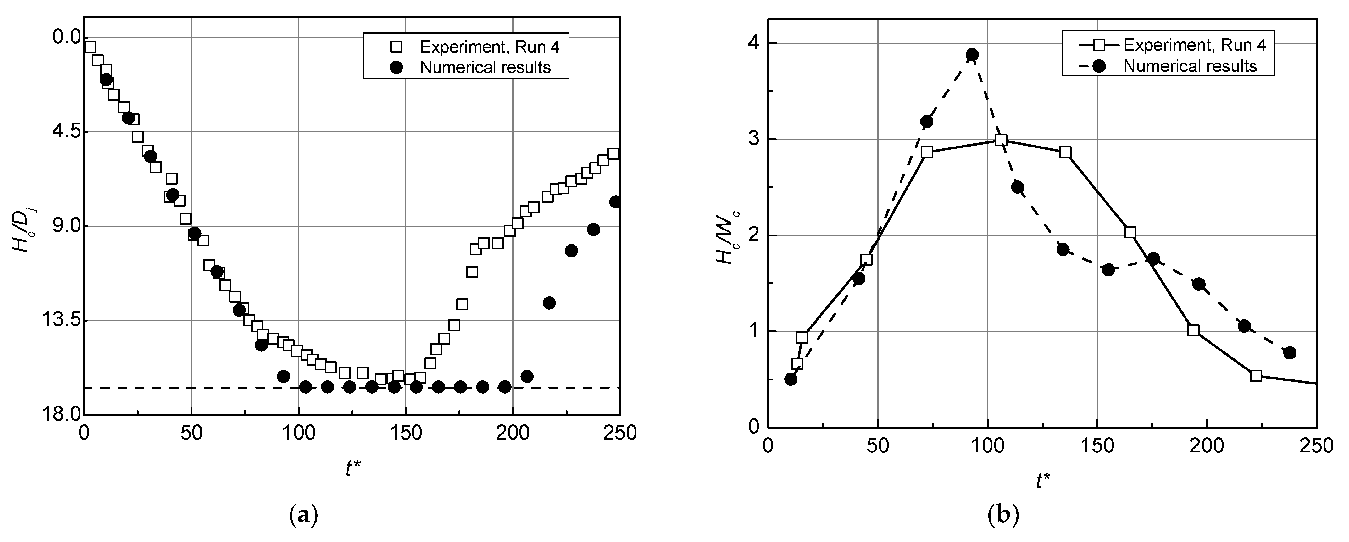
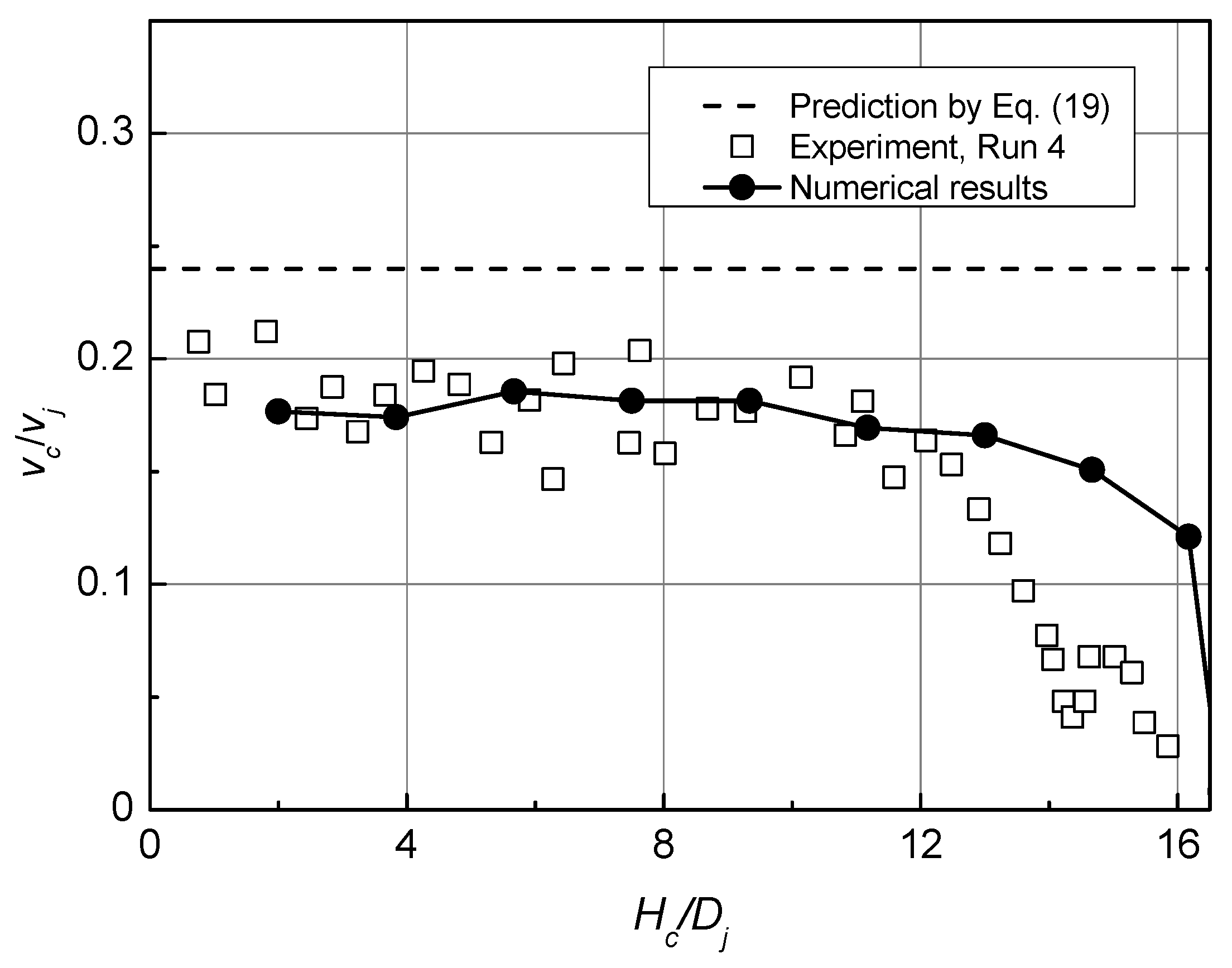
In the experimental work [12], by processing the images obtained by the neutron radiography method, the following quantitative characteristics of the process were established: the relative cavity depth, ; the cavity aspect ratio, ; and the relative cavity penetration velocity, . On the basis of these quantities, comparisons of the numerical predictions with the test data were carried out in the current work.
By postprocessing the distributions of volume fractions in the plane of symmetry (see Figure 9 and Figure 11) generated by the simulations at several sequential instants, the cavity penetration depth () and width () were determined in the following way. The cavity depth, , was determined as the difference between the initial melt level () and the height of the lowest point where the vapor volume fraction is . The cavity width, , was determined as the difference of the respective rightmost and leftmost points in the distribution of , taken below the initial melt level. The cavity penetration velocity, , was obtained by numerically differentiating the cavity depth, , as a function of time.
Figure 12 shows a comparison between numerical predictions and experimental data [12] on the relative cavity depth (a) and aspect ratio (b). It is necessary to emphasize that, in the simulation, the water jet diameter was mm, and the maximum possible cavity depth, corresponding to reaching the vessel bottom, was ; this value is indicated in Figure 12a by the horizontal dashed line.
In the course of the water jet’s interaction with the melt pool, the cavity created by the impact reached the vessel bottom, attaching to it for some time. The agreement of the predicted and measured cavity depth is quite good, especially up to the time . Later on, some discrepancies between the simulation and experiment data appear. In the simulation, the cavity reaches the vessel bottom by the time , its lower part spreads over the pool bottom, and the detachment of the cavity occurs at . In the experiment (Run 4 [12]), however, vertical cavity propagation slows down at time ; the cavity stays attached to the bottom for a short period only, detaching from the vessel bottom at .
Consider now the comparison of the calculated and experimental cavity aspect ratios. The larger vertical size of the cavity obtained numerically is also reflected in the cavity aspect ratio (Figure 12b): the calculated dependence has more pronounced maxima and is narrower than that measured experimentally. The experimental aspect ratio remains almost constant over some period when the cavity slows down and the maximum depth of jet penetration is reached. There is no such plateau in the simulation, meaning that the cavity is growing in the radial direction, displacing the melt along the vessel’s bottom. A possible reason for this discrepancy is that the wall friction acting on the melt due to its interaction with vessel walls is underestimated in the current numerical model, where turbulence effects are not taken into account explicitly.
In Figure 13, the experimental and predicted cavity penetration velocity, , normalized by the water jet velocity, , is plotted against the dimensionless cavity depth, . A theoretical estimate for the velocity, , obtained in [12] in nonboiling conditions for a shallow but infinitely wide cavity is as follows:
It is plotted in Figure 13 by the horizontal dashed line.
It can be seen that unstable melt–water interface propagation is observed in the experiments [12], with the fluctuation amplitude increasing with the cavity development. In the simulation, the cavity propagation velocity is almost constant up to the beginning of cavity deceleration, although some low-amplitude velocity oscillations are still observed.
The authors of Reference [12] estimated the error of the measurements performed to be 17%. Taking this into account, it can be stated that the results of the numerical simulation obtained in our work agree quite reasonably with the experimental data.
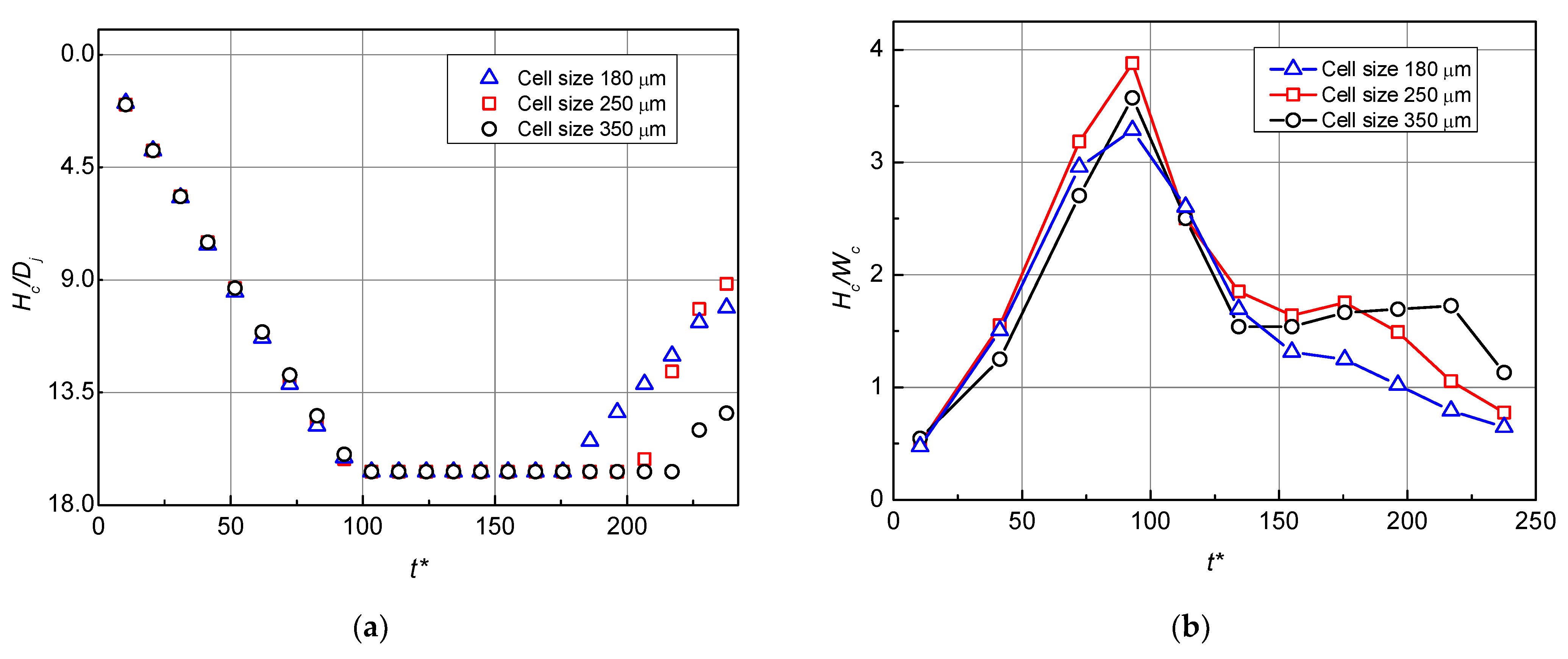
8. Study on Mesh Convergence
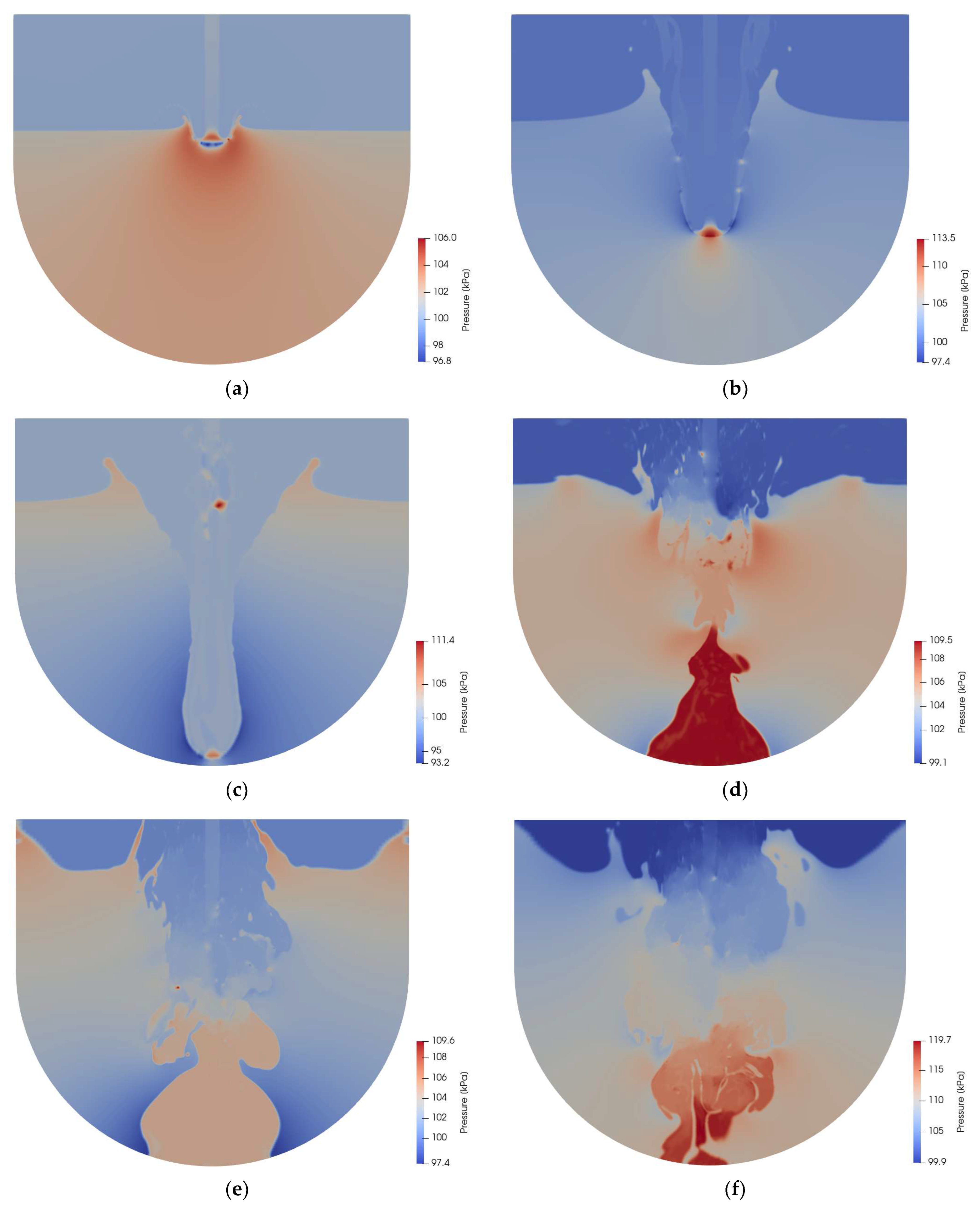
A feature of numerical simulations using the VOF method is that the evolution of all phases and the development of instabilities on the interfaces are modeled directly, without any averaging procedure. Refinement of the computational mesh not only increases the accuracy of finite-volume approximations but also allows one to resolve interface perturbations at smaller scales, affecting such processes as the fragmentation of fluids. For example, simulations of melt jet fragmentation in water performed on several meshes in [24] demonstrated that the jet breakup length becomes shorter, and more and more fine fragments appear with the decrease in the mesh cell size. In other words, no classical convergence to some mesh-independent solution can be expected in VOF simulations. However, a meaningful check is whether some integral features of the solutions become independent of the mesh size.
In order to evaluate the influence of the computational mesh, two additional simulations were performed for the same input parameters: one on a coarse mesh (the total number of cells was 878,800; the central area was covered with cubic cells with a side of µm), and another one on a refined mesh (the total number of cells was 10,198,656; the central area was covered with cubic cells with a side µm).
In Figure 14a,b, the time dependencies of the relative cavity depth, , and aspect ratio obtained on the three meshes with different cell sizes are presented. It can be seen that the initial penetration of the water jet into melt (up to ) proceeds at the same speed for all cell sizes; the same applies to the cavity aspect ratio (Figure 14b). This is expectable because, at this stage, the water jet remains stable, and the cavity boundary has a simple shape. Large differences occur as soon as the water jet becomes unstable, as well as when significant fragmentation of the melt begins. These differences are most visible in Figure 14b, starting from . By this time, the inertial stage of the cavity grows ends, and the influence of the vapor formation becomes significant. The higher values of the aspect ratio obtained on the coarse mesh after indicate that the cavity is relatively narrow: the vapor release intensity is smaller than that predicted on the two finer meshes.
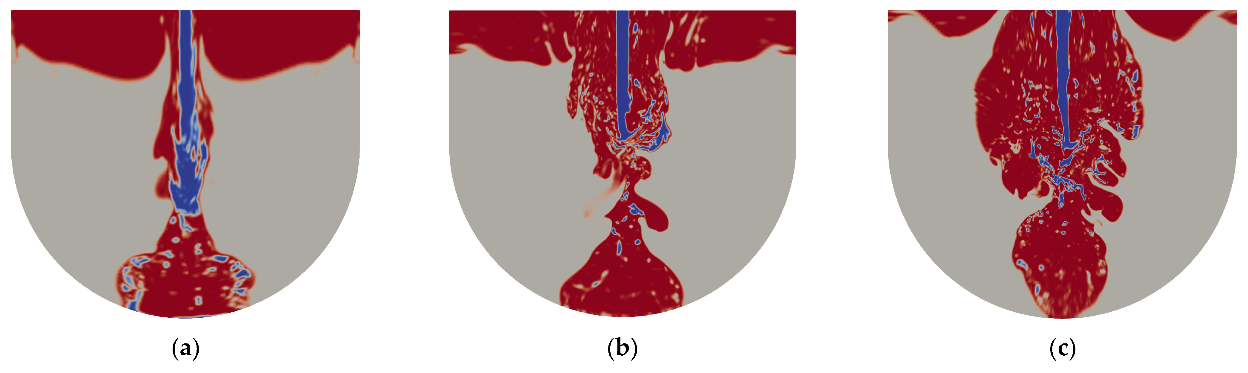
To further illustrate the influence of the mesh cell size, in Figure 15a–c, three solutions are presented, corresponding to the cross-section of the vessel at the same instant, . It can be seen that the cavity obtained on the coarse mesh (a) is significantly narrower than those obtained on the nominal (b) and refined (c) meshes. Evidently, the processes of water jet and melt fragmentation proceed more intensively in the latter two cases, resulting in better entrainment and more energetic boil-up of water; therefore, the vapor production rate that causes the widening of the cavity is higher.
It is important to note that, in the simulation on the finest mesh, water is practically not spreading along the vessel bottom after (Figure 15c), in contrast to the other two simulations performed on coarser meshes. This behavior most closely matches the experimental data.
9. Discussion
When a water jet penetrates a melt pool, a wide range of hydrodynamic and thermal phenomena arise that determine, in a coupled way, the melt–water interaction features and, in particular, the possible danger of this interaction to surrounding structures. Certainly, the VOF method is capable of describing the main processes involved, being a useful tool for the safety evaluation of various technological processes. In addition, it allows one to evaluate the results obtained by other methods. This is confirmed by the result obtained in the current work: it was shown numerically that the jet penetration depth is a linear function of its initial velocity, which agrees well with the experimental data, but shows the drawback of the theoretical estimate [12], which neglects the melt flow in the pool and drag between vapor and water.
The VOF method approximates the interfaces between phases by narrow transitional zones filled with some effective mixture, with the properties averaged between those of the phases. Special care is taken to control the transitional zone spreading only to few (typically, 2–3) mesh cells. This allows one to model the development of hydrodynamic instability of the interfaces from the wave formation and growth up to the separation of various-size droplets. Thus, in this method, no special (as a rule, empirical) models for such hydrodynamic processes as fragmentation or coagulation are introduced, which is an advantage with respect to Eulerian multi-fluid models depending heavily on the closures for interphase exchanges. Also, Eulerian models encounter significant difficulties in describing the polydisperse fragments, phase fragmentation, and coagulation, requiring the introduction of multiple phases according to (unknown beforehand) size distribution of fragments. The current study demonstrates the efficiency of the VOF approach in application to the problem of water jet interaction with melt pool, where fragmentation plays a key role.
Another attractive feature of the VOF method is the direct description of phase changes occurring in narrow transitional zones between the phases, without invoking any models for the interphase surface area. In VOF, the heat fluxes towards the interface (modeled by the thin transitional zone) are calculated directly from the heat transfer equation, while accounting for the current thermal gradients in the adjacent phases and thermal conductivities. The phase change rate in the near-interface cells is proportional to the superheating of the evaporating fluid; thus, the energy flux towards the interface is effectively converted to the appropriate mass flux of vapor. For the conditions considered in the current work, such an approach allowed the heat flux from the hot melt to be split into two parts: (i) heat going to subcooled water and (ii) heat going to the phase change.
The validity of the approach was confirmed by comparison with experiments [12,13,14] performed in a planar vessel (slice geometry). Since the vessel’s thickness is much smaller that its width and height, one would expect the damping of transverse flows and uniformity of all parameters in the transverse direction. However, the simulation results presented in Figure 9 and Figure 10 clearly demonstrate the asymmetry of phasic volume fractions at the late stage of the process. Evidently, the multiphase flow is three-dimensional, and the transverse flows intensify the mixing process.
The case of water jet interaction with melt studied in this work is featured by the vertical jet impact on the free surface of a melt pool. As a consequence, jet penetration into the melt results in the formation of a cavity filled with water jet core surrounded by vapor. Due to the momentum transferred by the impacting jet, the cavity propagates downwards, towards the vessel bottom, also extending in the horizontal direction and displacing the melt to the periphery. Our simulations demonstrated rather weak fragmentation and mixing of melt with water, which reduces the probability of their highly energetic (explosive) interaction. However, in the case of the SGTR accident, a high-pressure water jet is expected to be discharged from the ruptured tube well under the free level of molten metal, which makes the formation of a large gas cavity with high volume fraction of vapor practically improbable. In the steam generator, low-pressure melt flows between the heat exchange tubes, so that the discharged water becomes superheated (its temperature exceeds the phase change (boiling) temperature at the much lower system pressure). Therefore, water boil-up is going to occur on the outer boundary of the jet, so that the released vapor embraces the water jet core, separating it from the surrounding melt, while the water temperature drops to the boiling point. This process is significantly different from the practically isobaric interaction considered in the current work; it will be the focus of our future VOF studies.
10. Conclusions
The current study clearly demonstrated the high potential of the VOF method in application to complex multiphase flows with heat transfer and phase changes, without the involvement of empirical models for fragmentation rates, heat exchange coefficients, or evaporation rates.
This study revealed intrinsic limitations to the formation of the explosive three-phase mixture due to naturally arising phase separation that blocks the penetration of water droplets into heavy (and, therefore, highly inertial) melt. On the other hand, this blocking limits the fragmentation rate of the melt itself. This factor, thus, reduces the probability of steam explosions upon the interaction of water with hot metal melts.
The numerical tests performed when solving the problems of water jet interaction with heavy metal melt pool have shown that a prerequisite for adequate reproduction of the sophisticated multiphase flows is the use of fine-enough numerical meshes, allowing the flow details at small scales to be captured. On a coarse mesh, not only some fine details cannot be reproduced, but also the development of the interface instabilities responsible for water jet oscillations and fragmentation is delayed or suppressed completely. This affects such important features of the interaction as the cavity shape, depth, propagation speed, etc. It is important to note that, with the increase in the mesh resolution, more fine-scale flow details are reproduced in the simulations, making the classical “mesh-independent limit” unachievable. Therefore, VOF simulations of such complex flows as water–melt interactions must be validated against experimental data; such validations can help one to evaluate the adequate yet computationally feasible mesh size for the particular problem.
Thus, the novel results of direct numerical simulations presented in the paper are quite encouraging; they demonstrate the high potential of the VOF model for capturing the principal features and fine details of melt–water interactions. Future work will be devoted to the studies of water–melt interactions relevant to SGTR accidents in the fast neutron nuclear reactors with heavy coolant. In particular, of interest is the discharge of high-pressure water into heavy melt coolant. In such events, water boil-up occurs not only due to contact with hot melt, but also due to a rapid pressure drop, causing the volumetric boil-up of superheated liquid. Simulations of such transient processes would require the implementation of a nucleate boiling model, requiring an extension of the current approach where phase transitions occur only on the water–vapor interface tracked by the VOF method.
Author Contributions
Conceptualization, O.I.M.; methodology, S.E.Y. and V.I.M.; software, S.E.Y. and N.S.S.; validation, N.S.S.; writing—original draft preparation, N.S.S.; writing—review and editing, O.I.M., S.E.Y. and V.I.M. All authors have read and agreed to the published version of the manuscript.
Funding
This research was funded by the Russian Science Foundation (RSF), Grant No. 21-19-00709.
Data Availability Statement
Data are contained within the article.
Acknowledgments
Numerical simulations were performed on the high-performance computational platform provided by Joint Supercomputer Center (https://www.jscc.ru (accessed on 17 December 2023)).
Conflicts of Interest
The authors declare no conflict of interest. The funders had no role in the design of the study; in the collection, analyses, or interpretation of data; in the writing of the manuscript; or in the decision to publish the results.
Nomenclature
| void fraction, (–) | |
| volumetric phase change rate, kg/(m3·s) | |
| specific heat of evaporation, J/kg | |
| cell size, m | |
| surface curvature, m−1 | |
| thermal conductivity, W/(m·K) | |
| characteristic length, m | |
| film thickness, m | |
| dynamic viscosity, Pa·s | |
| density, kg/m3 | |
| interfacial tension, N/m | |
| viscous stress tensor, Pa | |
| specific heat capacity, J/(kg·K) | |
| nozzle diameter, m | |
| specific internal energy, J/kg | |
| surface tension force, N/m3 | |
| densimetric Froude number, (–) | |
| gravity acceleration, m/s2 | |
| cavity depth, m | |
| depth of melt pool, m | |
| vapor space height, m | |
| specific enthalpy, J/kg | |
| identity matrix | |
| total width of the vessel, m | |
| total number of phases | |
| space-averaged Nusselt number, (–) | |
| local Nusselt number, (–) | |
| pressure, Pa | |
| radius of the vessel bottom, m | |
| melt-water density ratio, (–) | |
| temperature, K | |
| time, s | |
| non-dimensional time, (–) | |
| velocity, m/s | |
| cavity penetration velocity, m/s | |
| jet velocity, m/s | |
| thickness of the vessel, m | |
| cavity width, m | |
| vapor film thickness, m | |
| Subscripts | |
| phase | |
| liquid | |
| melt | |
| saturation | |
| vapor | |
| water | |
| Cartesian coordinates | |
References
- Wang, G.A. Review of Research Progress in Heat Exchanger Tube Rupture Accident of Heavy Liquid Metal Cooled Reactors. Ann. Nucl. Energy 2017, 109, 1–8. [Google Scholar] [CrossRef]
- Dinh, T.N. Multiphase Flow Phenomena of Steam Generator Tube Rupture in a Lead-Cooled Reactor System: A Scoping Analysis. In Proceedings of the Societe Francaise d’Energie Nucleaire—International Congress on Advances in Nuclear Power Plants—ICAPP 2007, “The Nuclear Renaissance at Work”, Nice, France, 13–18 May 2007; Volume 5, pp. 2765–2775. [Google Scholar]
- Nigmatulin, R.I. Dynamics of Multiphase Media; Hemisphere: New York, NY, USA, 1991; Volume 1, ISBN 9780891163282. [Google Scholar]
- Iskhakov, A.S.; Melikhov, V.I.; Melikhov, O.I.; Yakush, S.E. Steam Generator Tube Rupture in Lead-Cooled Fast Reactors: Estimation of Impact on Neighboring Tubes. Nucl. Eng. Des. 2019, 341, 198–208. [Google Scholar] [CrossRef]
- Beznosov, A.V.; Pinaev, S.S.; Davydov, D.V.; Molodtsov, A.A.; Bokova, T.A.; Martynov, P.N.; Rachkov, V.I. Experimental Studies of the Characteristics of Contact Heat Exchange between Lead Coolant and the Working Body. At. Energy 2005, 98, 170–176. [Google Scholar] [CrossRef]
- Ciampichetti, A.; Bernardi, D.; Forgione, N. Analysis of the LBE-Water Interaction in the LIFUS 5 Facility to Support the Investigation of an SGTR Event in LFRs; ENEA Report RdS/2010/102; ENEA: Stockholm, Sweden, 2010. [Google Scholar]
- Pesetti, A.; Forgione, N.; Del Nevo, A. Water/Pb-Bi Interaction Experiments in LIFUS5/Mod2 Facility Modelled by SIMMER Code. In Proceedings of the 22nd International Conference on Nuclear Engineering (ICONE-2014), Prague, Czech Republic, 7–11 July 2014; Volume 3: Next Generation Reactors and Advanced Reactors; Nuclear Safety and Security. American Society of Mechanical Engineers: New York, NY, USA, 2014. [Google Scholar]
- Cheng, S.; Matsuba, K.; Isozaki, M.; Kamiyama, K.; Suzuki, T.; Tobita, Y. An Experimental Study on Local Fuel–Coolant Interactions by Delivering Water into a Simulated Molten Fuel Pool. Nucl. Eng. Des. 2014, 275, 133–141. [Google Scholar] [CrossRef]
- Cheng, S.; Matsuba, K.; Isozaki, M.; Kamiyama, K.; Suzuki, T.; Tobita, Y. The Effect of Coolant Quantity on Local Fuel–Coolant Interactions in a Molten Pool. Ann. Nucl. Energy 2015, 75, 20–25. [Google Scholar] [CrossRef]
- Cheng, S.; Matsuba, K.; Isozaki, M.; Kamiyama, K.; Suzuki, T.; Tobita, Y. SIMMER-III Analyses of Local Fuel-Coolant Interactions in a Simulated Molten Fuel Pool: Effect of Coolant Quantity. Sci. Technol. Nucl. Install. 2015, 2015, 964327. [Google Scholar] [CrossRef]
- Zhang, T.; Cheng, S.; Zhu, T.; Meng, C.; Li, X. A New Experimental Investigation on Local Fuel-Coolant Interaction in a Molten Pool. Ann. Nucl. Energy 2018, 120, 593–603. [Google Scholar] [CrossRef]
- Sibamoto, Y.; Kukita, Y.; Nakamura, H. Visualization and Measurement of Subcooled Water Jet Injection into High-Temperature Melt by Using High-Frame-Rate Neutron Radiography. Nucl. Technol. 2002, 139, 205–220. [Google Scholar] [CrossRef]
- Sibamoto, Y.; Kukita, Y.; Nakamura, H. Small-Scale Experiment on Subcooled Water Jet Injection into Molten Alloy by Using Fluid Temperature-Phase Coupled Measurement and Visualization. J. Nucl. Sci. Technol. 2007, 44, 1059–1069. [Google Scholar] [CrossRef]
- Sibamoto, Y.; Kukita, Y.; Nakamura, H. Simultaneous Measurement of Fluid Temperature and Phase during Water Jet Injection into High Temperature Melt. In Proceedings of the 11th International Topical Meeting on Nuclear Thermal-Hydraulics (NURETH-11), Avignon, France, 2–6 October 2005; Paper 181. pp. 1–15. [Google Scholar]
- Kolev, N.I. Volume 1. Fundamental. In Multiphase Flow Dynamics; Springer: New York, NY, USA, 2015; ISBN 9783319342559. [Google Scholar]
- Tobita, Y.; Kondo, S.; Yamano, H.; Morita, K.; Maschek, W.; Coste, P.; Cadiou, T. The Development of SIMMER-III, An Advanced Computer Program for LMFR Safety Analysis, and Its Application to Sodium Experiments. Nucl. Technol. 2006, 153, 245–255. [Google Scholar] [CrossRef]
- Ciampichetti, A.; Pellini, D.; Agostini, P.; Benamati, G.; Forgione, N.; Oriolo, F. Experimental and Computational Investigation of LBE–Water Interaction in LIFUS 5 Facility. Nucl. Eng. Des. 2009, 239, 2468–2478. [Google Scholar] [CrossRef]
- Prosperetti, A.; Tryggvason, G. Computational Methods for Multiphase Flow; Cambridge University Press: Cambridge, UK, 2007; ISBN 9780521847643. [Google Scholar]
- Tryggvason, G.; Scardovelli, R.; Zaleski, S. Direct Numerical Simulations of Gas-Liquid Multiphase Flow; Cambridge University Press: Cambridge, UK, 2011; ISBN 9780521782401. [Google Scholar]
- Hirt, C.; Nichols, B. Volume of Fluid (VOF) Method for the Dynamics of Free Boundaries. J. Comput. Phys. 1981, 39, 201–225. [Google Scholar] [CrossRef]
- Thakre, S.; Ma, W. 3D Simulations of the Hydrodynamic Deformation of Melt Droplets in a Water Pool. Ann. Nucl. Energy 2015, 75, 123–131. [Google Scholar] [CrossRef]
- Thakre, S.; Manickam, L.; Ma, W. A Numerical Simulation of Jet Breakup in Melt Coolant Interactions. Ann. Nucl. Energy 2015, 80, 467–475. [Google Scholar] [CrossRef]
- Kim, M.-S.; Bang, K.-H. Numerical Simulation of Kelvin–Helmholtz Instability and Boundary Layer Stripping for an Interpretation of Melt Jet Breakup Mechanisms. Energies 2022, 15, 7517. [Google Scholar] [CrossRef]
- Melikhov, V.I.; Melikhov, O.I.; Volkov, G.Y.; Yakush, S.E.; Salekh, B. Modelling of the Liquid Jet Discharge into a Liquid-Filled Space by the VOF Method. Therm. Eng. 2023, 70, 63–72. [Google Scholar] [CrossRef]
- Yakush, S.E.; Sivakov, N.S. Numerical Modeling of High-Temperature Melt Droplet Interaction with Water. Ann. Nucl. Energy 2023, 185, 109718. [Google Scholar] [CrossRef]
- Yakush, S.E.; Sivakov, N.S. Numerical Simulation of Water Jet Impact on Molten Material Layer. AIP Conf. Proc. 2023, 2872, 120052. [Google Scholar] [CrossRef]
- Huang, X.; Chen, P.; Yin, Y.; Pang, B.; Li, Y.; Gong, X.; Deng, Y. Numerical Investigation on LBE-Water Interaction for Heavy Liquid Metal Cooled Fast Reactors. Nucl. Eng. Des. 2020, 361, 110567. [Google Scholar] [CrossRef]
- Lin, Y.; Zhang, D.; Chen, Y.; Zhang, X.; Tian, W.; Qiu, S.; Su, G. Thermal-hydraulic Characteristics of Molten-Lead Bismuth Eutectic and Water Interaction. At. Energy Sci. Techn. 2023, 57, 56–65. [Google Scholar] [CrossRef]
- Yuan, J.; Liu, L.; Bao, R.; Luo, H.; Liu, M.; Gu, H. Three-Dimensional Numerical Simulation of the Interaction between High-Pressure Sub-Cooled Water Jet Impacting High-Temperature Liquid Lead-Bismuth Metal. Appl. Therm. Eng. 2023, 230, 120705. [Google Scholar] [CrossRef]
- Chen, G.; Nie, T.; Yan, X. An Explicit Expression of the Empirical Factor in a Widely Used Phase Change Model. Int. J. Heat Mass Transf. 2020, 150, 119279. [Google Scholar] [CrossRef]
- Open Source Field Operation and Manipulation (OpenFOAM). Available online: https://www.openfoam.com (accessed on 5 October 2023).
- Alexiades, V.; Solomon, A.D. Mathematical Modeling of Melting and Freezing Processes; Routledge: Oxfordshire, UK, 2018; ISBN 9780203749449. [Google Scholar]
- Welch, S.W.J.; Wilson, J. A Volume of Fluid Based Method for Fluid Flows with Phase Change. J. Comput. Phys. 2000, 160, 662–682. [Google Scholar] [CrossRef]
- Berenson, P.J. Film-Boiling Heat Transfer from a Horizontal Surface. J. Heat Transfer 1961, 83, 351–356. [Google Scholar] [CrossRef]
- Organisation for Economic Co-Operation and Development (OECD). Handbook on Lead-Bismuth Eutectic Alloy and Lead Properties, Materials Compatibility, Thermalhydraulics and Technologies; Nuclear Science; OECD: Paris, France, 2015; ISBN 9789264661066. [Google Scholar]
- Saito, M.; Sato, K.; Imahori, S. Experimental Study on Penetration Behavior of Water Jet into Freon-11 and Liquid Nitrogen. In Proceedings of the 25th National and 3rd International ISHMT-ASTFE Heat and Mass Transfer Conference (IHMTC-2019), Roorkee, India, 28–31 December 2019; American Nuclear Society: Houston, TX, USA, 1988; p. 173. [Google Scholar]
- Park, H.S.; Yamano, N.; Maruyama, Y.; Moriyama, K.; Yang, Y.; Sugimoto, J. Study on Energetic Fuel-Coolant Interaction in the Coolant Injection Mode of Contact. In Proceedings of the 6th International Conference on Nuclear Engineering (ICONE-6), San Diego, CA, USA, 10–14 May 1998. Paper ICONE-6091. [Google Scholar]
Figure 1.
One-dimensional Stefan problem: verification of numerical solutions on different meshes (dots) with analytical solution (solid line).
Figure 1.
One-dimensional Stefan problem: verification of numerical solutions on different meshes (dots) with analytical solution (solid line).

Figure 2.
Two-dimensional verification case: vapor volume fraction at times 0.1, 0.4, and 0.6 ms (left to right).
Figure 2.
Two-dimensional verification case: vapor volume fraction at times 0.1, 0.4, and 0.6 ms (left to right).

Figure 3.
Two-dimensional verification case: comparison with correlation [34].
Figure 3.
Two-dimensional verification case: comparison with correlation [34].

Figure 4.
Sketch of the computational domain: front and side view, along with geometric sizes.

Figure 5.
Side view of the computational domain covered with mesh.

Figure 6.
Two-dimensional water jet penetration into melt (water is shown by blue color, gray color denotes melt, red color denotes gas).
Figure 6.
Two-dimensional water jet penetration into melt (water is shown by blue color, gray color denotes melt, red color denotes gas).

Figure 7.
Comparison of the maximum jet penetration depth on the Froude number: dots correspond to numerical simulations performed with variable jet velocity, ; curves correspond to correlations from [12,36].

Figure 8.
Maximum jet penetration depth, , depends on the jet diameter, : dots correspond to numerical simulations at m/s; curves correspond to correlations from [12,36].

Figure 9.
Three-phase interaction in the and planes of symmetry: 10 (a), 45 (b), 95 (c), 130 (d), 170 (e), and 230 (f).
Figure 9.
Three-phase interaction in the and planes of symmetry: 10 (a), 45 (b), 95 (c), 130 (d), 170 (e), and 230 (f).


Figure 10.
Melt and water surfaces, case C1: (a), 75 (b), 105 (c), and 185 (d).

Figure 11.
Pressure field history in the plane of symmetry: (a), 45 (b), 95 (c), 130 (d), 170 (e), and 230 (f).
Figure 11.
Pressure field history in the plane of symmetry: (a), 45 (b), 95 (c), 130 (d), 170 (e), and 230 (f).

Figure 12.
Comparison of experimental [12] and calculated cavity development: (a) relative cavity depth, , with vessel bottom shown by the dashed line; and (b) cavity aspect ratio, .
Figure 12.
Comparison of experimental [12] and calculated cavity development: (a) relative cavity depth, , with vessel bottom shown by the dashed line; and (b) cavity aspect ratio, .

Figure 13.
Penetration velocity of the cavity bottom: comparison of the experimental [12] and numerical results.
Figure 13.
Penetration velocity of the cavity bottom: comparison of the experimental [12] and numerical results.

Figure 14.
Comparison of cavity geometry for different cell size: (a) relative cavity depth, ; and (b) cavity aspect ratio, .
Figure 14.
Comparison of cavity geometry for different cell size: (a) relative cavity depth, ; and (b) cavity aspect ratio, .

Figure 15.
Volume fraction distributions at calculated on meshes with different cell sizes: (a) µm, (b) µm, and (c) µm.
Figure 15.
Volume fraction distributions at calculated on meshes with different cell sizes: (a) µm, (b) µm, and (c) µm.


Table 1.
Phase properties.
| Phase | Density, kg/m3 | Specific Heat Capacity, J/(kg·K) | Dynamic Viscosity, Pa·s | Conductivity, W/(m·K) |
|---|---|---|---|---|
| Melt | 10,000 | 140 | 1.3 × 10⁻³ | 15 |
| Water | 1027 | 4181 | 0.3 × 10⁻³ | 0.65 |
| Vapor | variable | 1800 | 3.5 × 10⁻⁵ | 0.02 |
Table 2.
Two-dimensional simulation cases with different jet velocities.
| 2D Case | Jet Velocity (m/s) | Max Cavity Depth, | Predicted by Equation (16) | Rel. Diff (%) |
|---|---|---|---|---|
| 1 | 5 | 25.40 | 28.32 | 10.31 |
| 2 | 7.5 | 46.75 | 63.71 | 26.62 |
| 3 | 10 | 68.03 | 113.26 | 39.82 |
Disclaimer/Publisher’s Note: The statements, opinions and data contained in all publications are solely those of the individual author(s) and contributor(s) and not of MDPI and/or the editor(s). MDPI and/or the editor(s) disclaim responsibility for any injury to people or property resulting from any ideas, methods, instructions or products referred to in the content. |
© 2023 by the authors. Licensee MDPI, Basel, Switzerland. This article is an open access article distributed under the terms and conditions of the Creative Commons Attribution (CC BY) license (https://creativecommons.org/licenses/by/4.0/).
Share and Cite
MDPI and ACS Style
Yakush, S.E.; Sivakov, N.S.; Melikhov, O.I.; Melikhov, V.I. Numerical Modeling of Water Jet Plunging in Molten Heavy Metal Pool. Mathematics 2024, 12, 12. https://doi.org/10.3390/math12010012
AMA Style
Yakush SE, Sivakov NS, Melikhov OI, Melikhov VI. Numerical Modeling of Water Jet Plunging in Molten Heavy Metal Pool. Mathematics. 2024; 12(1):12. https://doi.org/10.3390/math12010012
Chicago/Turabian StyleYakush, Sergey E., Nikita S. Sivakov, Oleg I. Melikhov, and Vladimir I. Melikhov. 2024. "Numerical Modeling of Water Jet Plunging in Molten Heavy Metal Pool" Mathematics 12, no. 1: 12. https://doi.org/10.3390/math12010012
Note that from the first issue of 2016, this journal uses article numbers instead of page numbers. See further details here.