Bankruptcy Prediction for Sustainability of Businesses: The Application of Graph Theoretical Modeling

Abstract

Various methods are used when building bankruptcy prediction models. New sophisticated methods that are already used in other scientific fields can also be applied in this area. Graph theory provides a powerful framework for analyzing and visualizing complex systems, making it a valuable tool for assessing the sustainability and financial health of businesses. The motivation for the research was the interest in the application of this method rarely applied in predicting the bankruptcy of companies. The paper aims to propose an improved dynamic bankruptcy prediction model based on graph theoretical modelling. The dynamic model considering the causality relation between financial features was built for the period 2015–2021. Financial features entering the model were selected with the use of Domain knowledge approach. When building the model, the weights of partial permanents were proposed to determine their impact on the final permanent and the algorithm for the optimalisation of these weights was established to obtain the best performing model. The outcome of the paper is the improved dynamic graph theoretical model with a good classification accuracy. The developed model is applicable in the field of bankruptcy prediction and is an equivalent sophisticated alternative to already established models.

1. Introduction

Corporate bankruptcy is one of the significant issues which the companies in the economy are dealing with. It also affects the sustainable growth of business organizations. Corporate sustainability is considered to be a business and investment strategy that seeks to use the best business practices to meet and balance the needs of current and future stakeholders [1]. “The concept of financial sustainability refers to liquidity, long-term returns, growth potential, and the ability to withstand financial distress. Ignoring the signs of financial distress can lead to a situation in which bankruptcy is the only option” [2] (p. 3).

Therefore, it is very important to monitor the symptoms of financial distress in the early stages of their manifestations. As part of prevention and monitoring, it is possible to apply many models that are aimed at predicting the financial failure of companies.

These models were elaborated on a theoretical and practical level. Several of them have a basis in mathematical and statistical methods (mostly they are regression models or discriminant analysis models).

According to Ghodrati and Moghaddam [3], prediction models can be divided into statistical models, artificial intelligence models and theoretical models. Statistical models are based on discriminant analysis and can be univariate or multivariate. Multivariate statistical models include multivariate discriminant analysis models, linear probability models, Logit models and Probit models [4]. Sun et al. [5] point to three development tendencies in the application of bankruptcy prediction models: a transition from one-dimensional analysis of variables to multidimensional prediction, a shift from traditional statistical methods to machine learning methods that are based on artificial intelligence and more intensive involvement of hybrid and ensemble classifiers [6].

Aziz and Dar [7] divided prediction models into statistical models, artificially intelligent expert system models and theoretical models. According to the authors, statistical models focus on detecting bankruptcy symptoms, are based on accounting data, can be single-criteria or multi-criteria, and use standard procedures. Artificially intelligent expert system models have approximately the same characteristics as statistical models, however, they are highly dependent on software solutions. Theoretical models differ in their characteristics compared to the models that use artificial intelligence. Theoretical models reveal the qualitative causes of bankruptcy, are based on data that guarantee the confirmation of the cause of business failure according to the starting points in the theory, and use software products that are suitable for confirming the theoretical argument of business failure. According to the authors, the statistical models include: univariate analysis (financial analysis), multivariate discriminant analysis, linear probability model, Probit model and Logit model. Artificially intelligent expert system models include decision trees, neural networks, rough-set models and genetic algorithms. The last group of models is represented by entropy theory, gambler’s ruin theory, cash management theory and credit risk theories.

Another classification of techniques for developing bankruptcy prediction models is offered by Zhou and Lai [8], who classify them into statistical techniques, intelligent techniques and hybrid and ensemble models.

During the last decades, globalization in financial markets, increasing competition among firms, financial institutions, and organizations, as well as rapid economic, social, and technological changes have led to increased uncertainty and instability in the financial and business environment. As a result, the need for the application of effective methods of predicting the financial health of businesses, as well as the need for a comprehensive approach to solving the given problem, has increased. In this “new” reality, scientists as well as practitioners in the field of finance recognize that it is necessary to solve the problems of predicting the financial health of businesses through integrated and realistic approaches that are based on sophisticated techniques of quantitative analysis. The connection between financial theory and mathematical programming becomes highly significant. Optimization techniques, stochastic processes, simulation, forecasting, decision support systems, multivariate discriminant analysis, fuzzy logic, as well as others, are nowadays considered valuable prediction tools [9]. In their study, Balcaen and Ooghe [10] collected information on methods that can be applied in detecting possible financial failure of businesses. They investigated whether sophisticated and alternative methods can bring better results in the field of predicting the financial health of businesses compared to traditional statistical methods and in the end pointed out the significant benefits of these methods.

Sophisticated and alternative methods certainly include machine learning or artificial intelligence methods, which over time have become the standard in bankruptcy prediction, since statistical methods such as logistic regression and discriminant analysis have certain disadvantages, as they have strict prerequisites for their possible application. On the other hand, thanks to machine learning, it was possible to include new variables in the models that could not be included when applying statistical methods (for example, indicators of corporate governance, textual data from the annual report, data and findings about the company from newspaper articles, etc.). Machine learning models are also suitable for financial data because they do not rely on assumptions about the normal distribution of the data and allow to express non-linear relationships that probably exist between the probability of bankruptcy and various financial indicators [11]. According to Shi and Li [12], six of the ten most cited articles on bankruptcy prediction use some kind of machine learning technique. Neural network-based approaches seem to be particularly popular in this group of bankruptcy prediction methods.

An important group of methods that can be applied in predicting the bankruptcy of companies are mathematical programming methods. In the framework of mathematical programming, linear programming problem is especially important. The goal of linear programming is to find the optimal value so that the optimal solution is found for all ratios. The most widespread algorithm for solving linear programming problems is the simplex method. Multi-criteria linear programming method was used in bankruptcy prediction by Kwak et al. [13].

One of the mathematical programming methods is Data Envelopment Analysis (DEA) [14]. Compared to statistical methods, DEA is a relatively new, non-parametric method that represents one of many approaches to assessing the financial health of companies and their risk of bankruptcy. This method was first applied in 1978 by Charnes, Cooper and Rhodes. Depending on whether each unit of input brings the same amount of output or a variable amount of output, it is possible to divide DEA models into Constant Returns to Scale (DEA CRS) [15] and Variable Returns to Scale (DEA VRS) [16]. The DEA method has been used to predict the financial health of companies by Tone [17]; Wang et al. [18]; Paradi et al. [19]; Zhu [20]; Färe et al. [21]; Ahmad et al. [22] and many other authors.

Among the alternative methods that can be applied within the given issue, Cash Management Theory (CMT) can be mentioned. This method is focused on the short-term management of corporate cash balances [23,24]. Other methods include the Entropy theory, also called the balance sheet decomposition method. This procedure was described by Theil [25]. Pyramidal decompositions of the balance sheet, which help companies to maintain financial balance, were also proposed by Booth [26].

Multidimensional Scaling (MDS) was applied by Mar Molinero and Ezzamel [27] and subsequently by Neophytou and Mar Molinero [28]. They concluded that this method has a well-developed theoretical basis and also allows graphic display and visualization, which creates a prerequisite for a quick and concise analysis of the results.

An important alternative method is the Multi-Logit model. This method was first applied by Peel and Peel in 1988. This method makes it possible to use data from several years before failure and at the same time to differentiate between failing and non-failing enterprises several years before bankruptcy [29].

It is also possible to mention the CUSUM method, which is one of the most effective methods for determining the shift of a company from a state of financial health to a state of financial failure. For bankruptcy forecasting, the time series behavior of the variables for each failed and successful company is estimated using a Vector Autoregressions (VAR) model. If the time series of the company’s performance is positive and greater than a specific sensitivity parameter, the model indicates that there has been no change in the financial situation of the company. A negative score signals a change in the state of the firm [7].

A significant part of the current bankruptcy prediction research is represented by hybrid and ensemble models. Hybrid models combine two or more methods in order to use their capabilities to obtain a more powerful model [8]. Tsai [30] developed two-stage hybrid learning approach. In the first stage he focused on the instance selection task using clustering algorithm. The clustering results were than used as input for the second stage to construct a prediction model based on classification algorithm. Chen et al. [31] investigated the use of advanced hybrid Z-Score bankruptcy prediction model in selecting financial features of selected sample of listed companies. Among the ensemble models, AdaBoost can be mentioned. It is “a widely used ensemble algorithm that can be employed in conjunction with many other types of learning methods for base learners to improve their performance” [8] (p. 73). Heo and Yang [32] proved the usefulness of the bankruptcy prediction model using AdaBoost, especially in the construction industry. They used decision tree as a weak classifier for AdaBoost. Authors revealed that AdaBoost showed the best predictive accuracy compared to neural network, support vector machine, decision tree and Altman Z-Score. Zhou and Lai [8] revealed that AdaBoost algorithm combined with imputation methods has high predictive accuracy and they confirmed that it is a useful alternative for bankruptcy prediction with missing data.

One of the innovative methods which can be applied in bankruptcy prediction is graph theory. This method was applied in various fields such as mathematics, computer science, chemistry, physics, biology and sociology [33]. Its application has recently been extended to the field of business financial management—it has been applied in contractor selection [34], supply chain management [35,36], optimization problems—mutual debt compensation among firms [37] or big data default prediction [38].

According to Sun-Li [39] models based on static financial indicators are not able to efficiently predict bankruptcy over time. Therefore, recent and active area of research in bankruptcy prediction is dynamization of bankruptcy prediction models [40]. These models takes into account the dynamics of financial ratios [41] and the improving trends, so they may produce better forecast [40].

Currently, there are few studies dealing with the dynamic prediction of bankruptcy. Du Jardin [42] studied how to improve performance of traditional bankruptcy prediction models beyond one year. Based on the analysis of most frequent terminal failure processes of different groups of firms he constructed dynamic models with better prediction accuracy at a 3-year horizon than common models. Nyitrai [40] suggested dynamization approach to bankruptcy prediction models in which he used the minimum and maximum of financial indicators from the previous period as a benchmarks in order to provide a more comprehensive picture of the current financial performance of companies. The author concluded that “the proposed measure can increase the predictive performance of bankruptcy prediction models compared to models based solely on static financial ratios” [40] (p. 317). Korol [43] developed four dynamic bankruptcy prediction models for European enterprises with the use of fuzzy sets, recurrent and multilayer artificial neural networks, and decision trees. As inputs to these models, he calculated financial ratios 10 years prior to bankruptcy. The study revealed that “the dynamic models generate a smaller number of errors, and the decrease of effectiveness of such models is smaller with extending the forecast period than in the case of static models” [43] (p. 12). Shen et al. [44] proposed a new dynamic approach to financial distress prediction which combined multiple forecast results with a high latitude unbalanced data stream using the Adaptive Neighbor SMOTE-Recursive Ensemble Approach. Zhu et al. [45] used the Analytical hierarchy process and Entropy weight theory to determine an index system for the dynamic assessment of financial distress. They also constructed Probabilistic neural network-based dynamic financial distress prediction model. Choe and Garas [33] created a dynamic model to bankruptcy prediction based on the graph theoretical approach. They considered five selected financial ratios. The interactions of these financial ratios they converted into an adjacency matrix and its permanent was calculated as an index of a firm’s financial solvency. Their proposed model and Altman’s Z-Score model was applied to two sample groups and the accuracy of these two models in predicting financial solvency of companies was compared. They stated that the comparison of two models does not prove the superiority of one model over the other.

Graph theory is very rarely applied in the creation of dynamic bankruptcy prediction models. However, it provides a powerful framework for revealing relationships and connections between individual indicators. By visualizing these relationships and contexts, business managers can get a very good overview of how individual features are affected. This study aims to fill this research gap by proposing dynamic model based on graph theoretical approach especially within construction industry. We suppose that permanent functions of financial solvency matrices (as financial solvency indices) for different time periods do not have the same impact on the prediction of bankruptcy. Therefore, we suggest using the coefficients ${\alpha }_1,{\alpha }_2,\dots ,{\alpha }_s$ as weights of partial permanents to determine their impact on the final permanent. Then we establish an algorithm of optimization of these coefficients in order to obtain the best possible performing model, where the confusion matrix for calculating various metrics to evaluate the model is used.

Based on the above-mentioned the research question was as follows: Is graph theoretical approach appropriate alternative to established bankruptcy prediction methods?

The remainder of the paper is structured as follows: Section Material and methods describes research sample and financial features selected for the analysis. The main part of this section presents the process and methods applied when building graph theoretical model for bankruptcy prediction. Section Results offers results of graph theoretical model. Section Discussion compares results of the developed model with the benchmark in the given field as well as other sophisticated models and discusses them from the point of view of their performance as well as features selection methods. It also presents contribution, limitations and future direction of the research.

2. Material and Methods

Research sample consisted of 186 Slovak construction companies doing a business within SK NACE 42. Financial data of these companies for the years 2015–2021 were obtained from the Slovak Analytical Agency CRIF-Slovak Credit Bureau [46].

Construction industry was selected due to its high importance for the Slovak economy. In this regard Hafiz et al. [47] (p. 350) states that “the construction industry is one of the most vital to any country’s economy despite its high record of business failure”. The importance of the construction industry for the Slovak economy was emphasized by Strba [48]. According to this author while before the crisis the automotive industry was considered the main pillar of the Slovak economy, nowadays experts agree that the construction industry can help the revival of the economy in the recession the most. The construction industry is the main constructor of buildings and constructions, which are an important part of the creation of gross fixed capital in the Slovak economy. It also reacts immediately to changes in the economic cycle and has a multiplier effect on the development of other sectors. The construction industry consumes many different types of energy and mineral resources. It also produces a lot of construction waste and emissions. Therefore, compliance with the principles of sustainable development is very important for construction companies [49]. It is also important to note that the analyzed enterprises carry out the construction of large structures such as highways, roads, streets, bridges, tunnels, etc.

In this paper model based on graph theoretical approach was constructed and its results were compared with Altman model used in several studies as a benchmark. This model was first published in 1968 and predicted the probability of a company going bankrupt using a simple formula [32]. Altman initially included 22 financial indicators in his model, then limited them to the 5 most important ones [50]. In 1983, Altman compiled revised Z’-Score model for privately held firms. He replaced the market value of equity in the indicator $x_4$ with the book value of equity, changed the importance of the indicators as well as zones of discrimination [51]. Grey zone is typical for both Altman models. When the company falls in this category, it is not easy to predict the risk [32]. Altman model has been used as a benchmark in various studies. Kacer et al. [52] examined whether the Logit model which uses the same variables as the revised Altman Z’-Score model performs better. They found out that although Logit model achieves better classification performance, it is not statistically different from the revised Z’-Score model. Heo and Yang [32] revealed that machine learning-based algorithms achieve far greater prediction ability compared to Altman Z-Score. Ghosh and Kapil [53] compared results of bankruptcy prediction using Altman model, Data Envelopment analysis (DEA) model and neural network (NN) model. They found out that the cost of misclassification of the Z-Score model was high compared to the NN model and the DEA model. Therefore, they proposed the NN model and the DEA model to replace the Altman model for benchmarking purposes.

With respect to the analyzed sample of companies, the revised Z’-Score model for privately held firms [51] was used:

$$\begin{array}{c}\hfill Z^{\prime }=0.717x_1+0.847x_2+3.107x_3+0.420x_4+0.998x_5,\end{array}$$

(1)

where

• $x_1$ = working capital/total assets
• $x_2$ = retained earnings/total assets
• $x_3$ = earnings before interest and taxes/total assets
• $x_4$ = book value of equity/book value of total liabilities
• $x_5$ = sales/total assets
• $Z^{\prime }$ = overall revised index

Zones of discrimination:

$$\begin{array}{cccc}\hfill & \mathrm{for}{Z}^{\prime }<1.23\mathrm{the}\mathrm{company}\mathrm{belongs}\mathrm{to}\mathrm{the}\mathrm{distress}\mathrm{zone},\hfill & \hfill & \hfill \\ \hfill & \mathrm{for}1.23\le Z^{\prime }\le 2.9\mathrm{the}\mathrm{company}\mathrm{belongs}\mathrm{to}\mathrm{the}\mathrm{grey}\mathrm{zone},\hfill \\ \hfill & \mathrm{for}{Z}^{\prime }>2.9\mathrm{the}\mathrm{company}\mathrm{belongs}\mathrm{to}\mathrm{the}\mathrm{safe}\mathrm{zone}.\hfill & \hfill & \hfill \end{array}$$

(2)

In line with the approach of Heo and Yang [32] if the value of Altman Z’-Score fell in the grey zone, company was excluded from predictions.

Graph theoretical model was built in Python using the module named Scikit-learn. The assumption about whether the company is prosperous or not was made based on the criteria reflecting currently valid legislation and practice of Slovak businesses in determining their financial health. The company was classified as non-prosperous if the following three conditions were met [54]:

$$\begin{array}{cccc}\hfill \left(i\right)& \mathrm{EAT}<0,\hfill & \hfill & \hfill \\ \hfill \left(ii\right)& \mathrm{Current}\mathrm{ratio}<1,\hfill \\ \hfill \left(iii\right)& \mathrm{Financial}\mathrm{independence}\mathrm{ratio}<0.08.\hfill & \hfill & \hfill \end{array}$$

(3)

With respect to conditions (3) construction companies were divided into two groups. The first group consisted of 18 companies meeting the conditions (3), i.e., the group of non-prosperous companies. The second group consisted of 168 companies that do not meet the conditions (3), i.e., the group of prosperous companies.

Financial features for graph theoretical model were chosen based on the Domain knowledge approach as follows:

• Current Ratio = Current assets/Short-term liabilities (CR)
• Return on assets = EBIT/Total assets (ROA)
• Total assets turnover ratio = Total sales/Total assets (TATR)
• Total debt to total assets = Total debt/Total assets (TDTA)
• Credit period ratio = Short-term liabilities/Sales (CPR)

Selected features were the most frequently used ones in the previous studies (see Table 1), while features from all basic groups of financial health assessment (liquidity, profitability, capital structure, asset management) were included.

According to Dimitras et al. [55], Daubie and Meskens [56] and Akers et al. [57] one of the most commonly used financial ratios in bankruptcy prediction is Current ratio. Bredart [58] assumed that higher levels of liquidity will have a positive influence on the survival of businesses. Therefore, low liquidity generates higher risk of failure of companies. According to Hussain et al. [59] this ratio is negatively related to financial distress.

In addition to Current ratio, Chen et al. [31] added Total debt to total assets, and Total assets turnover ratio to the most used financial ratios in bankruptcy prediction. Von Thadden et al. [60] states that high debt structure will increase the company’s capital so it can give an indication of the ability to repay the total debt previously and can return the capital and generate new profit that can lower the probability of bankruptcy. Choe and Garas [33] argue that a low Asset turnover ratio indicates overproduction or average inventory management or poor practices, which is the main cause of business failure.

An important group of indicators represented in bankruptcy prediction models is profitability. According to Cultrera and Bredart [61] (p. 104) Return on assets “continually outperforms other profitability measures in assessing the risk of corporate failure”.

An important indicator of businesses’ financial health is Credit period ratio [62]. An alternative to the Credit period ratio applied by other authors is the Current liabilities to Sales ratio. This indicator was used by Karas and Srbova [63] as one of four indicators predicting bankruptcy of construction companies in the Czech Republic. The importance of monitoring this indicator in construction companies is also confirmed by Spicka [64]. According to this author, failure of construction companies is caused by high level of current liabilities.

Table 1. Previous studies of selected financial features.

Feature	Authors
CR	Li and Sun [65]; Chen and Du [66]; Kainulainen et al. [67]; Callejón et al. [68]; Lin et al. [69]; Režňáková and Karas [70]; Cultera and Bredart [61]; Liang et al. [71]; Zelenkov et al. [72]; Chou et al. [73]; Volkov et al. [74]; Son et al. [75]; Korol [43]; Farooq and Qamar [76]; Shen et al. [44]; Vuković et al. [77]; Tumpach et al. [78]; Yan et al. [79]; Chen et al. [31]; Rahman et al. [80]; Park et al. [81]; Pavlicko et al. [82]; Papíková and Papík [83]; Pavlicko and Mazanec [84]; Mousavi et al. [85]; Qian et al. [86]; Smith and Alvarez [87]
ROA	Altman [50]; Li and Sun [65]; Hu [88]; Chen and Du [66]; Premachandra et al. [89]; Kainulainen et al. [67]; Zhou et al. [90]; Cultera and Bredart [61]; Zelenkov et al. [72]; Volkov et al. [74]; Korol [43]; Farooq and Qamar [76]; Shen et al. [44]; Tumpach et al. [78]; Qian et al. [86]; Pavlicko and Mazanec [84]
TATR	Altman [50]; Platt and Platt [91]; Li and Sun [65]; Chen and Du [66]; Kainulainen et al. [67]; Tomczak et al. [92]; Režňáková and Karas [70]; Lin et al. [69]; Zelenkov et al. [72]; Du Jardin [93]; Chou et al. [73]; Vuković et al. [77]; Park et al. [81]; Chen et al. [31]; Rahman et al. [80]; Papíková and Papík [83]; Pavlicko and Mazanec [84]
TDTA	Šnircová [62]; Platt and Platt [91]; Premachandra et al. [89]; Chen and Du [66]; Hu [88]; Yeh et al. [94]; Kainulainen et al. [67]; Režňáková and Karas [70]; Lin et al. [69]; Zhou et al. [90]; Chou et al. [73]; Volkov et al. [74]; Zelenkov et al. [72]; Arroyave [95]; Le et al. [96]; Farooq and Qamar [76]; Vuković et al. [77]; Shen et al. [44]; Yan et al. [79]; Chen et al. [31]; Pavlicko et al. [82]; Park et al. [81]; Qian et al. [86]; Papíková and Papík [83]; Pavlicko and Mazanec [84]
CPR	Šnircová [62]; Mendes et al. [97]; Lin et al. [69]; Du Jardin [93]; Jabeur [98]; Wyrobek [99]; Karas and Srbova [63]; Shen et al. [44]; Park et al. [81]; Qian et al. [86]; Smith and Alvarez [87]

Source: authors.

Table 1. Previous studies of selected financial features.

Feature	Authors
CR	Li and Sun [65]; Chen and Du [66]; Kainulainen et al. [67]; Callejón et al. [68]; Lin et al. [69]; Režňáková and Karas [70]; Cultera and Bredart [61]; Liang et al. [71]; Zelenkov et al. [72]; Chou et al. [73]; Volkov et al. [74]; Son et al. [75]; Korol [43]; Farooq and Qamar [76]; Shen et al. [44]; Vuković et al. [77]; Tumpach et al. [78]; Yan et al. [79]; Chen et al. [31]; Rahman et al. [80]; Park et al. [81]; Pavlicko et al. [82]; Papíková and Papík [83]; Pavlicko and Mazanec [84]; Mousavi et al. [85]; Qian et al. [86]; Smith and Alvarez [87]
ROA	Altman [50]; Li and Sun [65]; Hu [88]; Chen and Du [66]; Premachandra et al. [89]; Kainulainen et al. [67]; Zhou et al. [90]; Cultera and Bredart [61]; Zelenkov et al. [72]; Volkov et al. [74]; Korol [43]; Farooq and Qamar [76]; Shen et al. [44]; Tumpach et al. [78]; Qian et al. [86]; Pavlicko and Mazanec [84]
TATR	Altman [50]; Platt and Platt [91]; Li and Sun [65]; Chen and Du [66]; Kainulainen et al. [67]; Tomczak et al. [92]; Režňáková and Karas [70]; Lin et al. [69]; Zelenkov et al. [72]; Du Jardin [93]; Chou et al. [73]; Vuković et al. [77]; Park et al. [81]; Chen et al. [31]; Rahman et al. [80]; Papíková and Papík [83]; Pavlicko and Mazanec [84]
TDTA	Šnircová [62]; Platt and Platt [91]; Premachandra et al. [89]; Chen and Du [66]; Hu [88]; Yeh et al. [94]; Kainulainen et al. [67]; Režňáková and Karas [70]; Lin et al. [69]; Zhou et al. [90]; Chou et al. [73]; Volkov et al. [74]; Zelenkov et al. [72]; Arroyave [95]; Le et al. [96]; Farooq and Qamar [76]; Vuković et al. [77]; Shen et al. [44]; Yan et al. [79]; Chen et al. [31]; Pavlicko et al. [82]; Park et al. [81]; Qian et al. [86]; Papíková and Papík [83]; Pavlicko and Mazanec [84]
CPR	Šnircová [62]; Mendes et al. [97]; Lin et al. [69]; Du Jardin [93]; Jabeur [98]; Wyrobek [99]; Karas and Srbova [63]; Shen et al. [44]; Park et al. [81]; Qian et al. [86]; Smith and Alvarez [87]

Source: authors.

2.1. Graph Theory Application

A graph is a mathematical structure of two ordered sets $G=(V,E)$, where V is a set of entities, typically called vertices which represent all kinds of objects such as computers, cities, companies, people and many more. The second set E represents a binary relation between the vertices such as connections between computers, roads between cities, cooperation between companies, human relationships and so on. Graphs have a natural pictorial representation, where elements of the vertex set V are drawn as points on a plane and the edge set E is drawn as a set of lines between the corresponding points. This pictorial representation of graphs can be helpful in modeling various real-life situations and is very useful in applications, when topological properties of graphs are investigated.

Graph theory provides useful mathematical models for variety of applications, such as communication networks, bioinformatics, chemistry, physics, sociology and so on. Only recently graph theoretical approach was used in the fields of quality management [100] and supply chain management [101].

In this paper a graph theoretical approach is used to evaluate financial solvency of companies. With selected financial ratios a financial solvency graph is constructed. The vertices of the graph represent selected financial ratios and edges represent the binary relation (the causality relation) between corresponding financial ratios. Pearson correlation coefficient (4) is the most commonly used formula to determine the strength of the causality relations (the linear correlation) between two sets of data.

$$\begin{array}{c}\hfill {\rho }_{x,y}=\frac{n\left(\sum xy\right)-\left(\sum x\right)\left(\sum y\right)}{\sqrt{[n\sum x^2-{(\sum x)}^2][n\sum y^2-{(\sum y)}^2]}}.\end{array}$$

(4)

For every edge in the financial solvency graph the Pearson’s correlation coefficient is used to determine a strength of the linear correlation between two financial ratios as the end vertices of the edge and this value of Pearson’s correlation coefficient represents the weight of that edge.

If G is a financial solvency graph with vertex set $V=\{v_1,v_2,\dots ,v_n\}$ and $w\left(v_i{v}_j\right)$ is a weight of the edge between the vertices $v_i$ and $v_j$ then the weighted adjacency matrix of G is the $n\times n$ matrix $A=\left(a_{ij}\right)$, where

$$\begin{array}{cc}\hfill a_{ij}& =\left\{\begin{array}{cc}w\left(v_i{v}_j\right),\hfill & \mathrm{if}{v}_i\mathrm{and}{v}_j\mathrm{are}\mathrm{adjacent},\hfill \\ 0,\hfill & \mathrm{otherwise}.\hfill \end{array}\right.\hfill \end{array}$$

(5)

Clearly, $w\left(v_i{v}_j\right)=w\left(v_j{v}_i\right)$, for $i,j=1,2,\dots ,n$ and $i\ne j$.

To develop a unique representation of the weighted adjacency matrix A of a financial solvency graph G the permanent function per(A) of matrix A is computed. The permanent function is a matrix function similar to the determinant. In contrast to the calculation of the determinant, when calculating the permanent of a matrix all negative signs (follow from permutations) are replaced by positive ones. This guarantees that multinomial function terms do not lose their significance due to a negative sign, but each term contributes to the overall system evaluation.

Valiant [102] defined the permanent of an $n\times n$ matrix $A=\left(a_{ij}\right)$ in the following way

$$\begin{array}{c}\hfill \mathrm{per}\left(A\right)={\displaystyle \sum _{\gamma \in S_n}}{\displaystyle \prod _{i=1}^n}{a}_{i,\gamma \left(i\right)},\end{array}$$

(6)

where the sum is taken over all elements $\gamma$ of the symmetric group $S_n$ (over all permutations of the numbers $1,2,\dots ,n$). All known methods for evaluating the permanent of an $n\times n$ matrix run in exponential time. Recently Glynn [103] introduced a new formula that has a computational efficiency $O\left(2^{n}n\right)$ and is given in the following form

$$\begin{array}{c}\hfill \mathrm{per}\left(A\right)=\left[{\displaystyle \sum _{\delta }}\left({\displaystyle \prod _{k=1}^n}{\delta }_k\right){\displaystyle \prod _{j=1}^n\sum _{i=1}^n}{\delta }_i{a}_{ij}\right]/2^{n-1},\end{array}$$

(7)

where the outer sum is over all $2^{n-1}$ vectors $\delta =({\delta }_1,\dots ,{\delta }_n)\in {\{\pm 1\}}^n$, with ${\delta }_1=1$.

Since only weighted adjacency matrices of the size $5\times 5$ are considered, it is possible to compute the permanent of a matrix $A=\left(a_{ij}\right)$ using the modification of the first row Laplace’s expansion by minors where

$$\begin{array}{c}\hfill \mathrm{per}\left(A\right)={\displaystyle \sum _{j=1}^5}{a}_{1j}\mathrm{per}\left(A_{1j}\right),\end{array}$$

(8)

where $A_{1j}$ is the submatrix (minor) of A obtained by removing the first row and j-th column. Then for computing the permanent of every submatrix $A_{1j}$, $j=1,2,\dots ,5$, the first row Laplace’s expansion is used again. The process is repeated until submatrices of the size $2\times 2$ are obtained. The permanent of a matrix of the size $2\times 2$ is the sum of products of the diagonal and off-diagonal elements.

2.2. Confusion Matrix

A confusion matrix is used to measure the performance of a classification model. It shows the number of correct and incorrect predictions for each class, which allows a better understanding of how well the model performs. The confusion matrix for binary classification contains the following information, see [104]:

• True Positive ($TP$) is the total counts of correctly classified positive examples.
• False Positive ($FP$) is the total counts of negative examples incorrectly classified as positive.
• False Negative ($FN$) is the total counts of positive examples incorrectly classified as negative.
• True Negative ($TN$): is the total counts of correctly classified negative examples.

The confusion matrix is very useful for calculating various metrics to evaluate the model, such as Accuracy, Precision, Recall and $\mathrm{F}1-\mathrm{score}$, see [104].

Accuracy expresses the number of correctly classified examples of all examples. This metric measures overall performance of the model.

$$\begin{array}{c}\hfill \mathrm{Accuracy}=\frac{TP+TN}{TP+FP+FN+TN}.\end{array}$$

(9)

Precision expresses the number of correctly classified positive examples of all positively classified examples. This metric measures model’s ability to separate positive and negative examples.

$$\begin{array}{c}\hfill \mathrm{Precision}=\frac{TP}{TP+FP}.\end{array}$$

(10)

Recall expresses the number of correctly classified positive examples of all positive examples in the test set. Recall measures model’s ability to identify positive examples.

$$\begin{array}{c}\hfill \mathrm{Recall}=\frac{TP}{TP+FN}.\end{array}$$

(11)

$\mathrm{F}1-\mathrm{score}$ provides a simple metric to compare models when the precision must be considered as well recall scores. It is expressed as the harmonic mean of the precision and recall scores and is given by the following formula:

$$\begin{array}{c}\hfill \mathrm{F}1-\mathrm{score}=\frac{2TP}{2TP+FP+FN}.\end{array}$$

(12)

2.3. Precision-Recall Curves

To illustrate the classification performance of prediction models, precision-recall curves (PRC) can be used. PRC plots all the pairs of precision and recall at each threshold. The main advantage of PRC over Receiver operating characteristic curve (ROC) is that the number of true-negative results is not used for constructing this curve. Therefore, when evaluating binary classifiers on imbalanced datasets, the usage of PRC is more informative compared to ROC curve [105]. In this research, similar to Miao and Zhu [105], after comparing all the F1-scores for the threshold set, the $\mathit{cut}-\mathit{off}$ with the largest F1-score was chosen as the optimum one.

2.4. Model Building

Let m be the number of companies. For every company $c\left(j\right)$, $j=1,2,\dots ,m$, the $n\times y$ matrix $M^{c\left(j\right)}$ of its financial data from the Slovak Analytical Agency CRIF is considered, where n is the number of selected financial ratios and y is the number of selected years, see

Table 2. Input matrix $M^{c\left(j\right)}$ for company $c\left(j\right)$.

	${\mathit{Year}}_1$	${\mathit{Year}}_2$	${\mathit{Year}}_3$	…	${\mathit{Year}}_{\mathit{y}-1}$	${\mathit{Year}}_{\mathit{y}}$
$Rati{o}_1$	$m_{11}$	$m_{12}$	$m_{13}$	…	$m_{1y-1}$	$m_{1y}$
$Rati{o}_2$	⋮	⋮	⋮	⋱	⋮	⋮
⋮
$Rati{o}_n$	$m_{n1}$	$m_{n2}$	$m_{n3}$	…	$m_{ny-1}$	$m_{ny}$

Source: authors.

.

The selected years are divided into s sliding periods each of b years such that, if the first period is $(yea{r}_1,yea{r}_2,\dots ,yea{r}_b)$, then the second period is $(yea{r}_2,yea{r}_3,\dots ,yea{r}_{b+1})$ and the last s period is $(yea{r}_{y-b+1},yea{r}_{y-b+2},\dots ,yea{r}_{y-1},yea{r}_y)$, $s=y-b+1$.

Then for every company $c\left(j\right)$, $j=1,2,\dots ,m$, and for every period of b consecutive selected years from the matrix $M^{c\left(j\right)}$ is constructed $n\times y$ matrix $B^{c\left(j\right)}$, see

Table 3. Matrix $B^{c\left(j\right)}$ with periods for company $c\left(j\right)$.

	2015	2016	2017	2018	2019	2020	2021
	Time Period 1
		Time Period 2
			Time Period 3
				Time Period 4
					Time Period 5
CR	$c{r}_{2015}$	…					$c{r}_{2021}$
ROA	$ro{a}_{2015}$	…					$ro{a}_{2021}$
TATR	$tat{r}_{2015}$	…					$tat{r}_{2021}$
TDTA	$tdt{a}_{2015}$	…					$tdt{a}_{2021}$
CPR	$cp{r}_{2015}$	…					$cp{r}_{2021}$

Selected years in sliding periods are marked with background colors. Source: authors.

. For every company and for every period, according to the Section 2.1, the $n\times n$ financial solvency matrix $A_i^{c\left(j\right)}$, $i=1,2,\dots ,s$, $j=1,2,\dots ,m$, is constructed as causal relationships between corresponding financial ratios.

Partial permanents of the financial solvency matrix $A_i^{c\left(j\right)}$ for every company and every period are calculated using the Algorithm 1.

Algorithm 1: Permanent of company $c\left(j\right)$

Data: Matrix $M^{c\left(j\right)}[1\dots n][1\dots y]$, Vector $\overrightarrow{\alpha }$, Scalar s $p_{c\left(j\right)}\leftarrow \overrightarrow{\alpha }·\overrightarrow{p{p}^{c\left(j\right)}}$;

If ${\alpha }_1,{\alpha }_2,\dots ,{\alpha }_s$ is a non-decreasing sequence of random real numbers from the interval $(0,1)$ that determine the impact of partial permanents on the final permanent, then for the final permanent of company $c\left(j\right)$, $j=1,2,\dots ,m$, we have

$$\begin{array}{c}\hfill p_{c\left(j\right)}={\displaystyle \sum _{i=1}^s}{\alpha }_{i}per\left(A_i^{c\left(j\right)}\right).\end{array}$$

(13)

By using the function precision_recall_curve from the library sklearn.metrics all the pairs of precision and recall at each threshold are calculated. According to the Section 2.3 the threshold with largest F1-score is selected as the $\mathit{cut}-\mathit{off}$.

If $p_{c\left(j\right)}\le \mathit{cut}-\mathit{off}$, then the model predicts that the company $c\left(j\right)$ is non-prosperous. Otherwise the company $c\left(j\right)$ is prosperous.

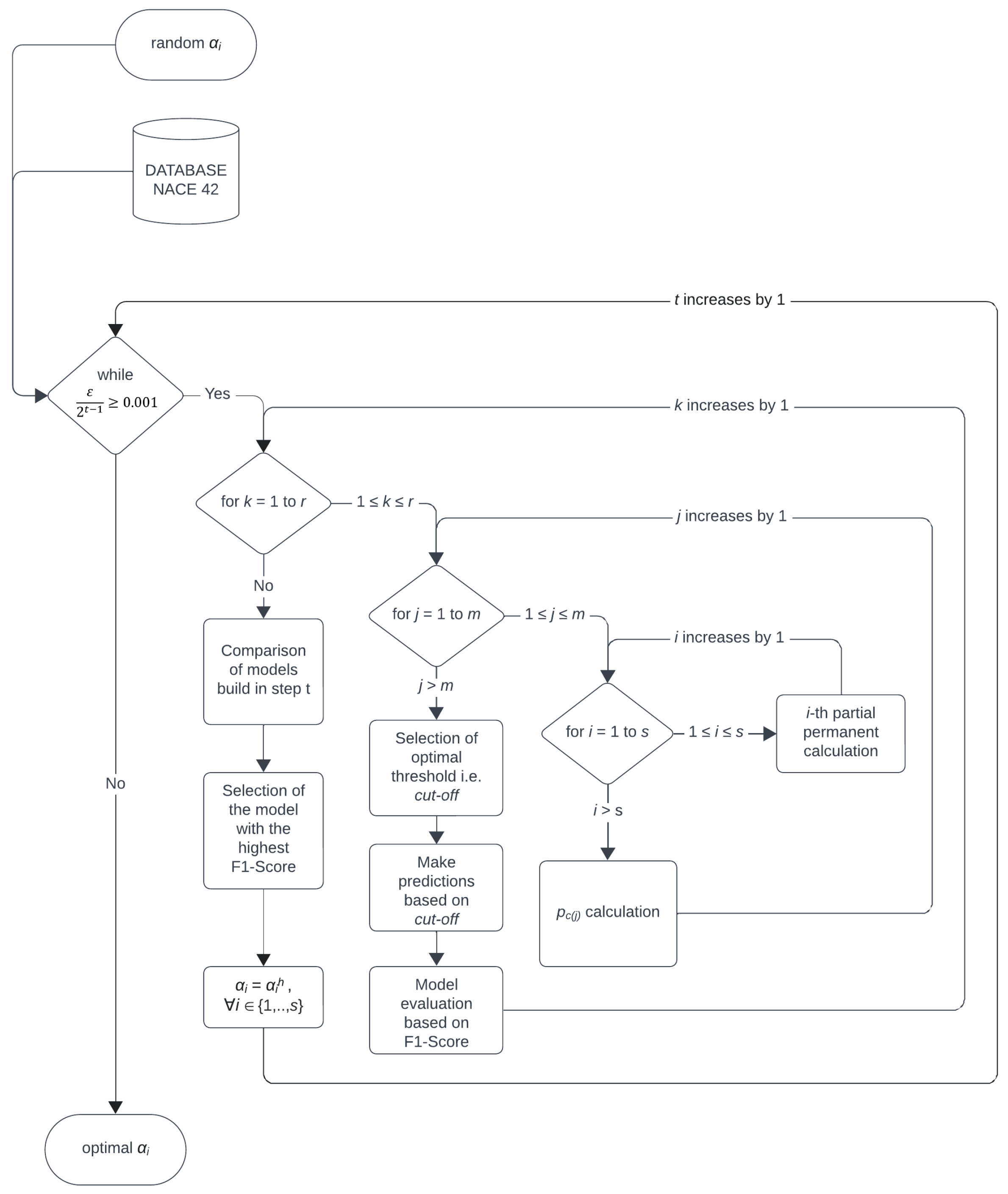
2.5. Optimization of Coefficients

This section deals with optimization of coefficients ${\alpha }_i$, $i=1,2,\dots ,s$, in order to obtain the best possible performing model. The optimization contains several steps and r iterations in each step, see Figure 1.

Step 1. Let $\epsilon$ be a random real number from the interval $(0,0.25)$.

1st iteration. For each ${\alpha }_i$, $i=1,2,\dots ,s$, a random real number ${\delta }_i^1\in (-\epsilon ,\epsilon )$ is chosen and ${\alpha }_i^1$ was defined as ${\alpha }_i^1=max\{min\{{\alpha }_i+{\delta }_i^1,1\},0\}$. Then the final permanent in the 1st iteration is as follows

$$p_{c\left(j\right)}^1=\sum _{i=1}^s{\alpha }_i^{1}per\left(A_i^{c\left(j\right)}\right).$$

For every company $c\left(j\right)$, $j=1,2,\dots ,m$ a prediction of bankruptcy is obtained and the optimal threshold with largest ${\mathrm{F}1}^1$-score was selected as the ${\mathit{cut}-\mathit{off}}^{\mathit{1}}$.

If $p_{c\left(j\right)}^1\le {\mathit{cut}-\mathit{off}}^{\mathit{1}}$, then the model predicts that the company $c\left(j\right)$ is non-prosperous. Otherwise it is not so.

kth iteration, $2\le k\le r$. For each ${\alpha }_i$, $i=1,2,\dots ,s$ a random real number ${\delta }_i^k\in (-\epsilon ,\epsilon )$ is chosen and ${\alpha }_i^k$ is calculated as ${\alpha }_i^k=max\{min\{{\alpha }_i+{\delta }_i^k,1\},0\}$. Then the final permanent in the kth iteration is given by

$$p_{c\left(j\right)}^k=\sum _{i=1}^s{\alpha }_i^{k}per\left(A_i^{c\left(j\right)}\right).$$

The optimal threshold with the largest ${\mathrm{F}1}^{\mathrm{k}}$-score was selected as the ${\mathit{cut}-\mathit{off}}^{\mathit{k}}$.

If $p_{c\left(j\right)}^k\le {\mathit{cut}-\mathit{off}}^{\mathit{k}}$, then the company $c\left(j\right)$ is non-prosperous. Otherwise the company $c\left(j\right)$ is prosperous.

After r iterations in the Step 1, the iteration with the largest F1-score is selected. If this iteration is denoted as hth iteration, then

$${\alpha }_i:={\alpha }_i^h,i=1,2,\dots ,s.$$

Step 2. t, $t\ge 2$. If $\frac{\epsilon }{2^{t-1}}<0.001$ then optimization is stopped and the Step $t-1$ is the last step for evaluation.

Otherwise, similarly to the Step $t-1$, r iterations are implemented in such a way that in the $k^{*}$th iteration for every ${\alpha }_i$, $i=1,2,\dots ,s$, a random real number ${\delta }_i^{k^{*}}\in \left(-\frac{\epsilon }{2^{t-1}},\frac{\epsilon }{2^{t-1}}\right)$ is chosen and ${\alpha }_i^{k^{*}}$ is defined as ${\alpha }_i^{k^{*}}=max\{min\{{\alpha }_i+{\delta }_i^{k^{*}},1\},0\}$. Then the final permanent in the $k^{*}$th iteration of the Step t is as follows

$$p_{c\left(j\right)}^{k^{*}}=\sum _{i=1}^s{\alpha }_i^{k^{*}}per\left(A_i^{c\left(j\right)}\right).$$

Similar to previous iterations, the optimal threshold with the largest ${\mathrm{F}1}^{{\mathrm{k}}^{*}}$-score was selected as the ${\mathit{cut}-\mathit{off}}^{{\mathit{k}}^{*}}$.

That way after r iterations in the Step t, the iteration with the highest F1-score is selected as $h^{*}$th iteration. Then

$${\alpha }_i:={\alpha }_i^{h^{*}},i=1,2,\dots ,s.$$

In the last step of this optimalization process the values of the coefficients ${\alpha }_i$, $i=1,2,\dots ,s$ are obtained and will be used as final values of the coefficients for the final model listed in the Section 2.4.

3. Results

When building graph theoretical model, analyzed years 2015–2021 were used to create s = 5 sliding periods each of $b=3$ years and for each company $c\left(j\right)$ the input matrix $M^{c\left(j\right)}$ gives the matrix $B^{c\left(j\right)}$, see Table 3. This approach was used to ensure dynamization of bankruptcy prediction model.

Results of descriptive statistics for individual features selected by Domain knowledge approach are stated in

Table 4. Descriptive statistics for selected financial features.

		2015	2016	2017	2018	2019	2020	2021
CR	Median	1.17	1.24	1.21	1.28	1.34	1.33	1.34
	Mean	1.92	1.84	1.90	1.73	1.92	2.11	2.34
ROA	Median	0.07	0.06	0.06	0.07	0.05	0.04	0.03
	Mean	0.11	0.08	0.08	0.11	0.05	0.05	0.02
TATR	Median	1.73	1.41	1.50	1.58	1.50	1.30	1.22
	Mean	1.89	1.67	1.68	1.69	1.66	1.43	1.40
TDTA	Median	0.69	0.65	0.61	0.61	0.58	0.58	0.60
	Mean	0.66	0.63	0.61	0.60	0.60	0.60	0.63
CPR	Median	0.33	0.33	0.32	0.29	0.29	0.31	0.33
	Mean	0.46	0.53	0.55	0.38	0.40	0.54	1.41

Source: authors.

.

The median of CR reaches slightly increasing values over the years. In 2021, it reached a value of 1.34, which can be evaluated positively. Even more significant increase in values can be seen in CR average, which reached a value of 2.34 in the last analyzed year. As CR reached an average value higher than 1.2, the given sample of companies can be considered less risky in terms of liquidity. It is also evidenced by the results of the assumption about non-prosperous companies. Regarding the results of ROA, it can be concluded that the analyzed companies are profitable, but the decrease in profitability from 7% to 2% and on average to 3% can be evaluated negatively. A negative development was also recorded in the TATR, which decreased over the years to a value of 1.22. It was caused by a decrease in sales, especially during the Covid-19 pandemic. At the beginning of the monitored period, the capital structure of the analyzed companies was 69%:31%, in favor of debt. However, at the end of the monitored period, there was an improvement in the share of equity by 9%. We can negatively evaluate the long CPR of 119 days, but the analyzed companies maintain this value of CPR during the entire monitored period, without significant fluctuations.

The created model (with input parameters) described in Section 2.4 was optimized according to Section 2.5, where $r=200$. The final values of the coefficients ${\alpha }_i$ obtained in Section 2.5 are as follows:

• ${\alpha }_1=0.0402$
• ${\alpha }_2=0.4142$
• ${\alpha }_3=0.1761$
• ${\alpha }_4=0.6334$
• ${\alpha }_5=0.8558$

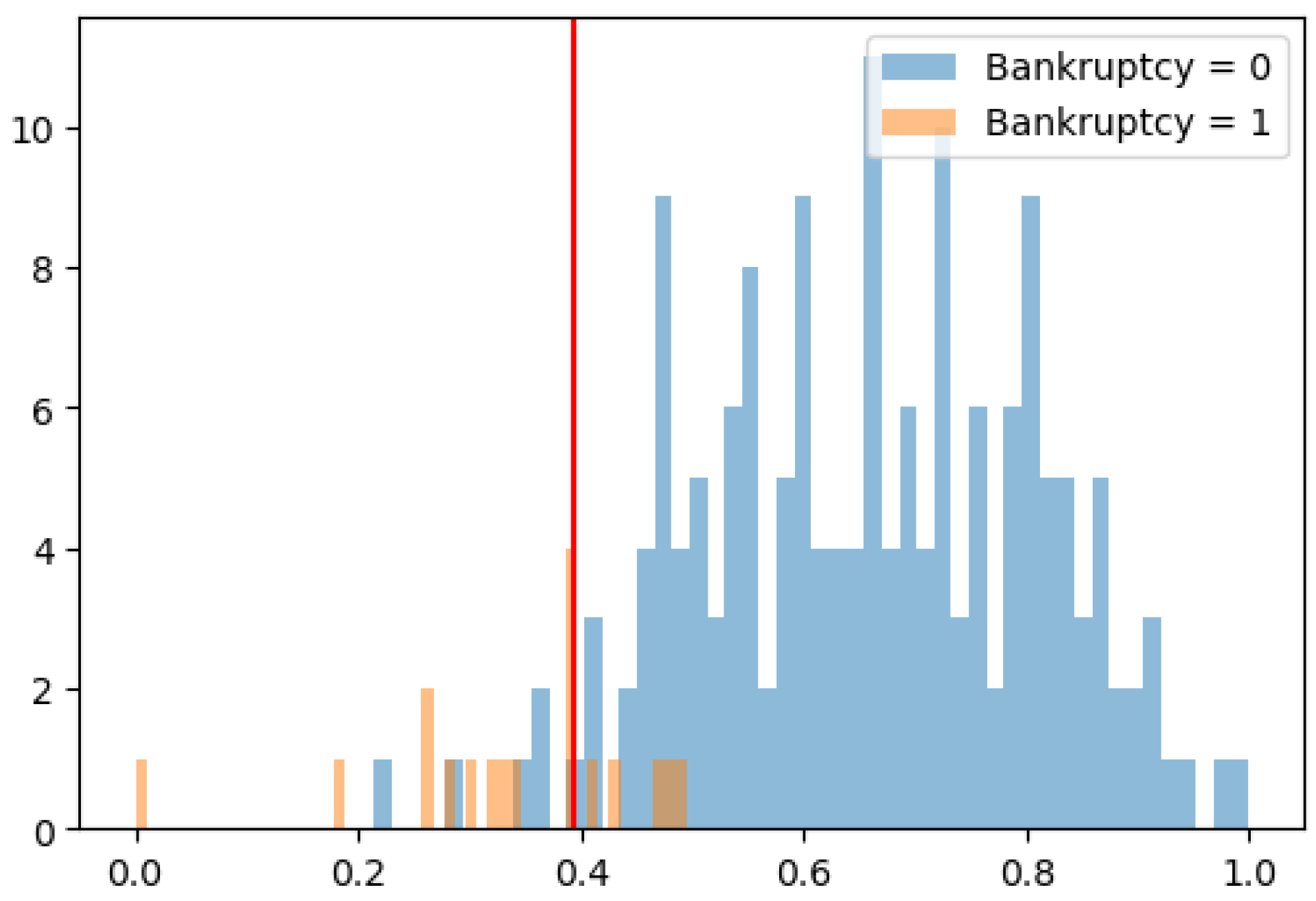
Bankruptcy predictions for companies $c\left(j\right)$ were determined according to the final model listed in the Section 2.4. The frequency of normalized permanents is illustrated on Figure 2. This figure also shows $\mathit{cut}-\mathit{off}$ (see Table 5) chosen based on procedure stated in Section 2.3. The model was evaluated using the metrics from the Section 2.2.

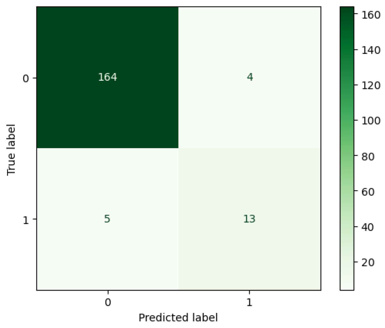
The confusion matrix of the Graph theoretical model (Figure 3) was created from the predicted and actual results.

The graph theoretical model correctly classified 177 companies. 13 of these companies were correctly classified as bankrupt and 164 companies as non-bankrupt. The model incorrectly classified 9 companies. 4 of these companies were incorrectly classified as bankrupt and 5 companies as non-bankrupt.

The obtained metrics of the Graph theoretical model are as follows:

Table 5. Metrics of the Graph theoretical approach.

Metric	Value
Accuracy	0.9516
Precision	0.7647
Recall	0.7222
F1-score	0.7429
$\mathit{cut}-\mathit{off}$	0.3928

Source: authors.

Table 5. Metrics of the Graph theoretical approach.

Metric	Value
Accuracy	0.9516
Precision	0.7647
Recall	0.7222
F1-score	0.7429
$\mathit{cut}-\mathit{off}$	0.3928

Source: authors.

4. Discussion

Construction industry is one of the vital ones within the economy of every country. An important part of this industry are companies that build large structures such as highways, roads, etc. When predicting bankruptcy, the position of these companies is crucial, because a threat to their financial health would negatively affect the development of the business environment and transport infrastructure in the given region. When building bankruptcy prediction model for construction industry, the innovative approach based on graph theoretical modeling was used. Graph theoretical model achieved classification accuracy 0.9516, while the F1-score of the model was 0.7429, see

Table 6. Performance of models.

	Graph Theoretical Model	Altman Z’-Score
Accuracy	0.9516	0.4409
F1-score	0.7429	0.2239

Source: authors.

. This model can be applied as early warning model not only for Slovak construction companies but also for construction companies operating under similar conditions such as transition economies.

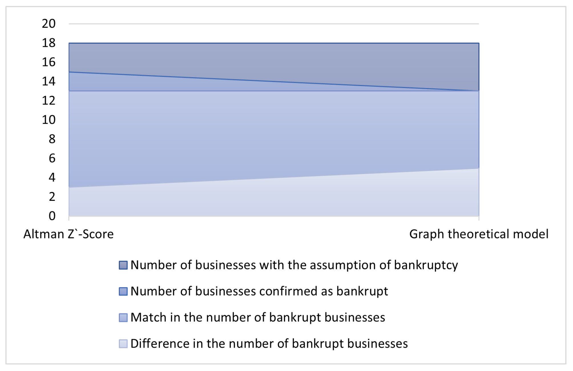
The performance of the model was compared with the Altman model, which is considered a benchmark in the given field. Altman Z’-Score achieved lower classification accuracy in both metrics. Similar results were achieved by several other authors [32,53,106] when comparing results of sophisticated models with Altman model. However, if we compare number of businesses confirmed as bankrupt, we can see that from 18 businesses with the assumption of bankruptcy, graph theoretical model confirmed 13 bankrupt businesses, while Altman model confirmed 15 bankrupt businesses, see Figure 4. These results can be justified by the fact that the Altman model was primarily designed to predict bankruptcy.

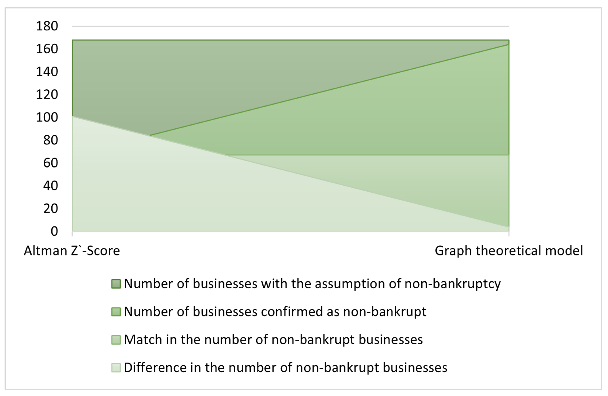
On the other hand, if we compare results of confirmed non-bankrupt businesses, they are different. From 168 businesses with the assumption of non-bankruptcy, graph theoretical approach confirmed 164 businesses, while Altman model confirmed 67 businesses, see Figure 5.

Graph theoretical model was developed for the time period of 7 years, while other models were constructed for a different period of time. Nevertheless, classification accuracy of graph theoretical model is comparable to other sophisticated models. For example Korol et al. [43] constructed four dynamic models applying different methods. The dynamic multilayer neural network model achieved the highest classification accuracy 93.4%, the best result of recurrent neural network model was 95.2%, model based on fuzzy sets achieved the best classification accuracy of 96.2% and the highest classification accuracy of decision tree model was 93%. Zhu et al. [45] determined an index system for the dynamic evaluation of financial distress with the use of analytical hierarchy process and entropy weight theory. Then they used probabilistic neural network to construct a dynamic prediction model. The average accuracy of the model after considering timelines achieved 95.03%.

In this paper we came to the finding that when combining Domain knowledge features selection with bankruptcy prediction using graph theoretical approach, the model with good classification accuracy can be developed. A similar result was achieved by Zhou et al. [90], who found out that Domain knowledge combined with genetic algorithms brings good results in the classification accuracy of corporate bankruptcy. Sinha and Zhao [107] revealed that incorporation of Domain knowledge significantly improves classifier performance with respect to both misclassification cost and AUC. Based on these findings it seems that Domain knowledge combined with some sophisticated method can ensure good classification accuracy of developed model.

Managerial implications of the research lie in the fact that indicators selected by the Domain knowledge approach are suitable for predicting bankruptcy in the financial management of Slovak construction companies. Regarding contribution to literature, the possibility of using the graph theoretical approach in bankruptcy prediction was confirmed. In this context, it would be necessary to reevaluate the previous classifications of bankruptcy prediction methods and create a new classification framework. Limitation of the research was the amount of data, which was limited by the need to find a sample of companies that operated on the market during the entire analyzed period. Due to the higher fluctuation in the given sector, the resulting number of enterprises was lower than expected, and thus the number of bankrupt enterprises was also lower. Therefore, in the future research we will try to obtain a larger amount of data in order to create a balanced sample. We will also examine the performance of the graph theoretical model when selecting features using data mining techniques and compare it with the Domain knowledge approach. It is necessary to further apply the graph theoretical approach and confirm the justification of this method in the classification tree of bankruptcy prediction methods.

References

- Artiach, T.; Lee, D.; Nelson, D.; Walker, J. The determinants of corporate sustainability performance. Account. Financ. 2010, 50, 31–51. [Google Scholar] [CrossRef]
- Srebro, B.; Mavrenski, B.; Bogojevic Arsic, V.; Knezevic, S.; Milasinovic, M.; Travica, J. Bankruptcy Risk Prediction in Ensuring the Sustainable Operation of Agriculture Companies. Sustainability 2021, 13, 7712. [Google Scholar] [CrossRef]
- Ghodrati, H.; Moghaddam, A.H.M. A study of the accuracy of bankruptcy prediction models: Altman, Shirata, Ohlson, Zmijewsky, CA score, Fulmer, Springate, Farajzadeh genetic, and Mckee genetic models for the companies of the stock exchange of tehran. Am. J. Sci. Res. 2012, 59, 55–67. [Google Scholar]
- Araghi, K.; Makvandi, S. Evaluating Predictive power of Data Envelopment Analysis Technique Compared with Logit and Probit Models in Predicting Corporate Bankruptcy. Aust. J. Bus. Manag. Res. 2012, 2, 38–46. [Google Scholar]
- Sun, J.; Li, H.; Huang, Q.H.; He, K.Y. Predicting Financial Distress and Corporate Failure: A Review from the State-of-the-art Definitions, Modeling, Sampling, and Featuring Approaches. Knowl.-Based Syst. 2014, 57, 41–56. [Google Scholar] [CrossRef]
- Mihalovic, M. Applicability of Scoring Models in Firms’ Default Prediction. The Case of Slovakia. Politická Ekon. 2018, 66, 689–708. [Google Scholar] [CrossRef]
- Aziz, A.; Dar, H. Predicting Corporate Bankruptcy: Where We Stand? Corp. Gov. 2006, 6, 18–33. [Google Scholar] [CrossRef]
- Zhou, L.; Lai, K.K. AdaBoost Models for Corporate Bankruptcy Prediction with Missing Data. Comput. Econ. 2017, 50, 69–94. [Google Scholar] [CrossRef]
- Zopounidis, C.; Doumpos, M. Multi-criteria Decision Aid in Financial Decision Making: Methodologies and Literature Review. J. -Multi-Criteria Decis. Anal. 2012, 11, 167–186. [Google Scholar] [CrossRef]
- Balcaen, S.; Ooghe, H. 35 Years of Studies on Business Failure: An Overview of the Classical Statistical Methodologies and Their Related Problems; Working Papers of Faculty of Economics and Business Administration; Ghent University: Ghent, Belgium, 2004. [Google Scholar]
- Giordani, P.; Jacobson, T.; Schedvin, E.; Villani, M. Taking the Twists into Account: Predicting Firm Bankruptcy Risk with Splines of Financial Ratios. J. Financ. Quant. Anal. 2014, 49, 1071–1099. [Google Scholar] [CrossRef]
- Shi, Y.; Li, X. An overview of bankruptcy prediction models for corporate firms: A systematic literature review. Intang. Cap. 2019, 15, 114–127. [Google Scholar] [CrossRef]
- Kwak, W.; Shi, Y.; Kou, G. Bankruptcy prediction for Korean firms after the 1997 financial crisis: Using a multiple criteria linear programming data mining approach. Rev. Quant. Financ. Account. 2012, 38, 441–453. [Google Scholar] [CrossRef]
- Horváthová, J.; Mokrišová, M. Risk of Bankruptcy, Its Determinants and Models. Risks 2018, 6, 117. [Google Scholar] [CrossRef]
- Charnes, A.; Cooper, W.W.; Rhodes, E. Measuring the efficiency of decision making units. Eur. J. Oper. Res. 1978, 2, 429–444. [Google Scholar] [CrossRef]
- Banker, R.D.; Charnes, A.; Cooper, W.W. Some models for estimating technical scale inefficiences in Data Envelopment Analysis. Manag. Sci. 1984, 30, 1078–1092. [Google Scholar] [CrossRef]
- Tone, K. A Slacks-Based Measure of Efficiency in Data Envelopment Analysis. Eur. J. Oper. Res. 2001, 130, 498–509. [Google Scholar] [CrossRef]
- Wang, Y.M.; Chin, K.S.; Yang, J.B. Measuring the performances of decision-making units using geometric average efficiency. J. Oper. Res. Soc. 2007, 58, 929–937. [Google Scholar] [CrossRef]
- Paradi, J.C.; Rouatt, S.; Zhu, H. Two-stage evaluation of bank branch efficiency using data envelopment analysis. Omega 2011, 39, 99–109. [Google Scholar] [CrossRef]
- Zhu, J. DEA based benchmarking models. In Data Envelopment Analysis. International Series in Operations Research & Management, Science; Zhu, J., Ed.; Springer: Boston, MA, USA, 2015; Volume 221. [Google Scholar]
- Färe, R.; Grosskopf, S.; Margaritis, D. Advances in Data Envelopment Analysis; World Scientific Publishing Company: Singapore, 2015. [Google Scholar]
- Ahmad, M.F.; Ishtiaq, M.; Hamid, K.; Khurram, M.U.; Nawaz, A. Data Envelopment Analysis and Tobit Analysis for Firm Efficiency in Perspective of Working Capital Management in Manufacturing Sector of Pakistan. Int. J. Econ. Financ. Issues 2017, 7, 706–713. [Google Scholar] [CrossRef]
- Black, F.; Scholes, M. The valuation of option contracts and a test of market efficiency. J. Financ. 1973, 27, 399–417. [Google Scholar] [CrossRef]
- Kordestani, G.; Bakhtiari, M.; Biglari, V. Ability of combinations of cash flow components to predict financial distress. Bus. Theory Pract. 2011, 12, 277–285. [Google Scholar] [CrossRef]
- Theil, H. On the Use of Information Theory Concepts in the Analysis of Financial Statements. Manag. Sci. 1969, 15, 459–480. [Google Scholar] [CrossRef]
- Booth, P.J. Decomposition measure and the prediction of financial failure. J. Bus. Financ. Account. 1983, 10, 67–82. [Google Scholar] [CrossRef]
- Mar Molinero, C.; Ezzamel, M. Multidimensional scaling applied to corporate failure. Omega 1991, 19, 259–274. [Google Scholar] [CrossRef]
- Neophytou, E.; Molinero, C.M. Predicting corporate failure in the UK: A multidimensional scaling approach. J. Bus. Financ. Account. 2004, 31, 677–710. [Google Scholar] [CrossRef]
- Klieštik, T.; Klieštiková, J.; Kováčová, M.; Švábová, L.; Valášková, K.; Vochozka, M.; Oláh, J. Prediction of Financial Health of Business Entities in Transition Economies; Addleton Academic Publishers: New York, NY, USA, 2018. [Google Scholar]
- Tsai, C.F. Two-stage hybrid learning techniques for bankruptcy prediction. Stat. Anal. Data Min. 2020, 13, 565–572. [Google Scholar] [CrossRef]
- Chen, Y.-S.; Lin, C.-K.; Lo, C.-M.; Chen, S.-F.; Liao, Q.-J. Comparable Studies of Financial Bankruptcy Prediction Using Advanced Hybrid Intelligent Classification Models to Provide Early Warning in the Electronics Industry. Mathematics 2021, 9, 2622. [Google Scholar] [CrossRef]
- Heo, J.; Yang, J.Y. AdaBoost based bankruptcy forecasting of Korean construction companies. Appl. Soft Comput. 2014, 24, 494–499. [Google Scholar] [CrossRef]
- Choe, K.; Garas, S. The graph theoretical approach to bankruptcy prediction. J. Account. Manag. 2021, 11, 47–57. [Google Scholar] [CrossRef]
- Darvish, M.; Yasaei, M.; Saeedi, A. Application of the graph theory and matrix methods to contractor ranking. Int. J. Proj. Manag. 2009, 27, 610–619. [Google Scholar] [CrossRef]
- Wagner, S.M.; Neshat, N. Assessing the vulnerability of supply chains using graph theory. Int. J. Prod. Econ. 2010, 126, 121–129. [Google Scholar] [CrossRef]
- Singh, R.K.; Kumar, P. Measuring the flexibility index for a supply chain using graph theory matrix approach. J. Glob. Oper. Strateg. Sourc. 2020, 13, 56–69. [Google Scholar] [CrossRef]
- Gazda, V.; Horvath, D.; Resovsky, M. An application of graph theory in the process of mutual debt compensation. Acta Polytech. Hung. 2015, 12, 7–24. [Google Scholar]
- Yildirim, M.; Okay, F.Y.; Özdemir, S. Big data analytics for default prediction using graph theory. Expert Syst. Appl. 2021, 176, 114840. [Google Scholar] [CrossRef]
- Sun, J.; Li, H. Dynamic financial distress prediction using instance selection for the disposal of concept drift. Expert Syst. Appl. 2011, 38, 2566–2576. [Google Scholar] [CrossRef]
- Nyitrai, T. Dynamization of bankruptcy models via indicator variables. Benchmarking Int. J. 2019, 26, 317–332. [Google Scholar] [CrossRef]
- Niklis, D.; Doumpos, M.; Zopounidis, C. Combining market and accounting-based models for credit scoring using a classification scheme based on support vector machines. Appl. Math. Comput. 2014, 234, 69–81. [Google Scholar] [CrossRef]
- Du Jardin, P. Bankruptcy prediction using terminal failure processes. Eur. J. Oper. Res. 2015, 242, 286–303. [Google Scholar] [CrossRef]
- Korol, T. Dynamic Bankruptcy Prediction Models for European Enterprises. J. Risk Financ. Manag. 2019, 12, 185. [Google Scholar] [CrossRef]
- Shen, F.; Liu, Y.; Wang, R. A dynamic financial distress forecast model with multiple forecast results under unbalanced data environment. Knowl. Based Syst. 2020, 192, 105365. [Google Scholar] [CrossRef]
- Zhu, J.; Zhu, H.; Lin, N.; Farouk, A. A Dynamic Prediction Model of Financial Distress in the Financial Sharing Environment. Discret. Dyn. Nat. Soc. 2023, 2023, 6259689. [Google Scholar] [CrossRef]
- CRIF. Financial Statements of Analyzed Businesses; Slovak Credit Bureau, s.r.o.: Bratislava, Slovakia, 2022. [Google Scholar]
- Hafiz, A.; Lukumon, O.; Muhammad, B.; Olugbenga, A.; Hakeem, O.; Saheed, A. Bankruptcy Prediction of Construction Businesses: Towards a Big Data Analytics Approach. In Proceedings of the 2015 IEEE First International Conference on Big Data Computing Service and Applications, San Francisco, CA, USA, 30 March–3 April 2015; IEEE Computer Society: Washington, DC, USA, 2015; pp. 347–352. [Google Scholar]
- Strba, M. Rozhýbe Stavebníctvo po Koronakríze Slovenskú Ekonomiku? [Will the Construction Industry Drive the Slovak Economy after the Corona Crisis?]. 2020. Available online: https://podnikatelskecentrum.sk/rozhybe-stavebnictvo-po-koronakrize-slovensku-ekonomiku/ (accessed on 15 July 2023).
- MTSR. Ročenka Slovenského Stavebníctva 2019 [Yearbook of the Slovak Construction 2019]; Ministry of Transport of the Slovak Republic: Bratislava, Slovakia, 2019; Available online: https://www.mindop.sk/ministerstvo-1/vystavba-5/stavebnictvo/dokumenty-a-materialy/rocenky-stavebnictva (accessed on 22 March 2023).
- Altman, E.I. Financial Ratios, Discriminant Analysis and the Prediction of Corporate Bancruptcy. J. Financ. 1968, 23, 589–609. [Google Scholar] [CrossRef]
- Altman, E.I. Predicting Financial Distress of Companies: Revisiting the Z-Score and Zeta Models; Working Paper; Stern School of Business, New York University: New York, NY, USA, 2000. [Google Scholar]
- Kacer, M.; Ochotnicky, P.; Alexy, M. The Altman’s Revised Z’-Score Model, Non-financial Information and Macroeconomic Variables: Case of Slovak SMEs. Ekon. Cas. 2019, 67, 335–366. [Google Scholar]
- Ghosh, A.; Kapil, S. Is Altman’s Model efficient in predicting bankruptcy?—A comparison among the Altman Z-score, DEA, and ANN models. J. Inf. Optim. Sci. 2022, 43, 1191–1207. [Google Scholar] [CrossRef]
- Valaskova, K.; Svabova, L.; Durica, M. Verifikácia predikčných modelov v podmienkach slovenského poľnohospodárskeho sektora [Verification of prediction models in conditions of the Slovak agricultural sector]. Ekon. Manag. Inovace [Econ. Manag. Innov.] 2017, 9, 30–38. Available online: http://emijournal.cz/wp-content/uploads/2017/12/03_verifikacia-predik%C4%8Dn%C3%BDch-modelov.pdf (accessed on 13 May 2023).
- Dimitras, A.I.; Slowinski, R.; Susmaga, R.; Zapounidis, C. Business failure prediction using rough sets. Eur. J. Oper. Res. 1999, 114, 263–280. [Google Scholar] [CrossRef]
- Daubie, M.; Meskens, N. Bankruptcy prediction: Literature survey of the last ten years. Belg. J. Oper. Res. Stat. Comput. Sci. 2001, 41, 43–58. [Google Scholar]
- Akers, M.; Bellovary, J.; Giacomino, D. A review of bankruptcy prediction studies: 1930 to present. J. Financ. Educ. 2007, 33, 1–42. [Google Scholar]
- Bredart, X. Bankruptcy Prediction Model: The Case of the United States. Int. J. Econ. Financ. 2014, 6, 1–7. [Google Scholar] [CrossRef]
- Hussain, M.; Nassir, A.; Shamsher, M.; Hassan, T. Prediction of Corporate Financial Distress of PN4 Companies in Malaysia: A Logistic Model Approach. J. Restruct. Financ. 2005, 2, 143–155. [Google Scholar] [CrossRef]
- Von Thadden, E.L.; Berglöf, E.; Roland, G. The design of corporate debt structure and bankruptcy. Rev. Financ. Stud. 2010, 23, 2648–2679. [Google Scholar] [CrossRef]
- Cultrera, L.; Bredart, X. Bankruptcy prediction: The case of Belgian SMEs. Rev. Account. Financ. 2016, 15, 101–119. [Google Scholar] [CrossRef]
- Šnircová, J. Možnosti prognózovania finančnej situácie podnikov v slovenskej ekonomike [Possibilities of forecasting the financial situation of companies in the Slovak economy]. BIATEC 1997, 5, 15–22. [Google Scholar]
- Karas, M.; Srbova, P. Predicting bankruptcy in construction business: Traditional model validation and formulation of a new model. J. Int. Stud. 2019, 12, 283–296. [Google Scholar] [CrossRef]
- Spicka, J. The financial condition of the construction companies before bankruptcy. Eur. J. Bus. Manag. 2013, 5, 160–170. [Google Scholar]
- Li, H.; Sun, J. Ranking-order case-based reasoning for financial distress prediction. Knowl.-Based Syst. 2008, 21, 868–878. [Google Scholar] [CrossRef]
- Chen, W.-S.; Du, Y.-K. Using neural networks and data mining techniques for the financial distress prediction model. Expert Syst. Appl. 2009, 36, 4075–4086. [Google Scholar] [CrossRef]
- Kainulainen, L.; Yu, Q.; Miche, Y.; Eirola, E.; Séverin, E.; Lendasse, A. Ensembles of Locally Linear Models: Application to Bankruptcy Prediction. In Proceedings of the 2010 International Conference on Data Mining, DMIN 2010, Las Vegas, NV, USA, 12–15 July 2010; pp. 280–286. [Google Scholar]
- Callejón, A.M.; Casado, A.M.; Fernández, M.A.; Peláez, J.I. A System of Insolvency Prediction for industrial companies using a financial alternative model with neural networks. Int. J. Comput. Intell. Syst. 2013, 6, 29–37. [Google Scholar] [CrossRef]
- Lin, F.; Liang, D.; Yeh, C.-C.; Huang, J.-C. Novel feature selection methods to financial distress prediction. Expert Syst. Appl. 2014, 41, 2472–2481. [Google Scholar] [CrossRef]
- Režňáková, M.; Karas, M. Bankruptcy Prediction Models: Can the Prediction Power of the Models be Improved by Using Dynamic Indicators? Procedia Econ. Financ. 2014, 12, 565–574. [Google Scholar] [CrossRef]
- Liang, D.; Lu, C.-C.; Tsai, C.-F.; Shih, G.-A. Financial ratios and corporate governance indicators in bankruptcy prediction: A comprehensive study. Eur. J. Oper. Res. 2016, 252, 561–572. [Google Scholar] [CrossRef]
- Zelenkov, Y.; Fedorova, E.; Chekrizov, D. Two-step classification method based on genetic algorithm for bankruptcy forecasting. Expert Syst. Appl. 2017, 88, 393–401. [Google Scholar] [CrossRef]
- Chou, C.-H.; Hsieh, S.-C.; Qiu, C.-J. Hybrid genetic algorithm and fuzzy clustering for bankruptcy prediction. Appl. Soft Comput. 2017, 56, 298–316. [Google Scholar] [CrossRef]
- Volkov, A.; Benoit, D.F.; van den Poel, D. Incorporating sequential information in bankruptcy prediction with predictors based on Markov for discrimination. Decis. Support Syst. 2017, 98, 59–68. [Google Scholar] [CrossRef]
- Son, H.; Hyun, C.; Phan, D.; Hwang, H.J. Data analytic approach for bankruptcy prediction. Expert Syst. Appl. 2019, 138, 112816. [Google Scholar] [CrossRef]
- Farooq, U.; Qamar, M.A.J. Predicting multistage financial distress: Reflections on sampling, feature and model selection criteria. J. Forecast. 2019, 38, 632–648. [Google Scholar] [CrossRef]
- Vuković, B.; Milutinović, S.; Milićević, N.; Jakšić, D. Corporate Bankruptcy Prediction: Evidence from Wholesale Companies in the Western European Countries. J. Econ. 2020, 68, 477–498. [Google Scholar]
- Tumpach, M.; Surovičová, A.; Juhászová, Z.; Marci, A.; Kubaščíková, Z. Prediction of the Bankruptcy of Slovak Companies Using Neural Networks with SMOTE. J. Econ. 2020, 68, 1021–1039. [Google Scholar] [CrossRef]
- Yan, D.; Chi, G.; Lai, K.K. Financial Distress Prediction and Feature Selection in Multiple Periods by Lassoing Unconstrained Distributed Lag Non-linear Models. Mathematics 2020, 8, 1275. [Google Scholar] [CrossRef]
- Rahman, M.; Sa, C.L.; Masud, M.A.K. Predicting Firms’ Financial Distress: An Empirical Analysis Using the F-Score Model. J. Risk Financ. Manag. 2021, 14, 199. [Google Scholar] [CrossRef]
- Park, M.S.; Son, H.; Hyun, C.; Hwang, H.J. Explainability of machine learning models for bankruptcy prediction. IEEE Access 2021, 9, 124887–124899. [Google Scholar] [CrossRef]
- Pavlicko, M.; Durica, M.; Mazanec, J. Ensemble Model of the Financial Distress Prediction in Visegrad Group Countries. Mathematics 2021, 9, 1886. [Google Scholar] [CrossRef]
- Papíková, L.; Papík, M. Effects of classification, feature selection, and resampling methods on bankruptcy prediction of small and medium-sized enterprises. Intell. Syst. Account. Financ. Manag. 2022, 29, 254–281. [Google Scholar] [CrossRef]
- Pavlicko, M.; Mazanec, J. Minimalistic Logit Model as an Effective Tool for Predicting the Risk of Financial Distress in the Visegrad Group. Mathematics 2022, 10, 1302. [Google Scholar] [CrossRef]
- Mousavi, M.M.; Ouenniche, J.; Tone, K. A dynamic performance evaluation of distress prediction models. J. Forecast. 2023, 42, 756–784. [Google Scholar] [CrossRef]
- Qian, H.; Wang, B.; Yuan, M.; Gao, S.; Song, Y. Financial distress prediction using a corrected feature selection measure and gradient boosted decision tree. Expert Syst. Appl. 2022, 190, 116202. [Google Scholar] [CrossRef]
- Smith, M.; Alvarez, F. Predicting Firm-Level Bankruptcy in the Spanish Economy Using Extreme Gradient Boosting. Comput. Econ. 2022, 59, 263–295. [Google Scholar] [CrossRef]
- Hu, Y.-C. Bankruptcy prediction using ELECTRE-based single-layer perceptron. Neurocomputing 2009, 72, 3150–3157. [Google Scholar] [CrossRef]
- Premachandra, I.M.; Bhabra, G.S.; Sueyoshi, T. DEA as a tool for bankruptcy assessment: A comparative study with logistic regression technique. Eur. J. Oper. Res. 2009, 193, 412–424. [Google Scholar] [CrossRef]
- Zhou, L.; Lu, D.; Fujita, H. The performance of corporate financial distress prediction models with features selection guided by domain knowledge and data mining approaches. Knowl.-Based Syst. 2015, 85, 52–61. [Google Scholar] [CrossRef]
- Platt, H.D.; Platt, M.B. Understanding differences between financial distress and bankruptcy. Rev. Appl. Econ. 2006, 2, 141–157. [Google Scholar]
- Tomczak, S.; Przybyslawski, B.; Górski, A. Comparative analysis of the bankruptcy prediction models. In Information Systems Architecture and Technology: The Use of IT Models for Organization Management; Part, 3; Wilimowska, Z., Borzemski, L., Grzech, A., Światek, J., Eds.; Oficyna Wydawnicza Politechniki Wrocawskiej: Wroclaw, Poland, 2012; pp. 157–166. [Google Scholar]
- Du Jardin, P. Dynamics of firm financial evolution and bankruptcy prediction. Expert Syst. Appl. 2017, 75, 25–43. [Google Scholar] [CrossRef]
- Yeh, C.C.; Chi, D.J.; Hsu, M.F. A hybrid approach of DEA, rough set and support vector machines for business failure prediction. Expert Syst. Appl. 2010, 37, 1535–1541. [Google Scholar] [CrossRef]
- Arroyave, J. A comparative analysis of the effectiveness of corporate bankruptcy prediction models based on financial ratios: Evidence from Colombia. J. Int. Stud. 2018, 11, 273–287. [Google Scholar] [CrossRef]
- Le, T.; Vo, B.; Fujita, H.; Nguyen, N.-T.; Baik, S.W. A fast and accurate approach for bankruptcy forecasting using squared logistics loss with GPU-based extreme gradient boosting. Inf. Sci. 2019, 494, 294–310. [Google Scholar] [CrossRef]
- Mendes, F.; Duarte, J.; Vieira, A.; Gaspar-Cunha, A. Feature selection for bankruptcy prediction: A multi-objective optimization approach. In Soft Computing in Industrial Applications. Advances in Intelligent and Soft Computing; Gao, X.Z., Gaspar-Cunha, A., Köppen, M., Schaefer, G., Wang, J., Eds.; Springer: Berlin/Heidelberg, Germany, 2010; pp. 109–115. [Google Scholar]
- Jabeur, S.B. Bankruptcy prediction using Partial Least Squares Logistic Regression. J. Retail. Consum. Serv. 2017, 36, 197–202. [Google Scholar] [CrossRef]
- Wyrobek, J. Predicting Bankruptcy at Polish Companies: A Comparison of Selected Machine Learning and Deep Learning Algorithms. Crac. Rev. Econ. Manag. 2018, 6, 41–60. [Google Scholar] [CrossRef]
- Grover, S.; Agrawal, V.; Khan, I. A digraph approach to TQM evaluation of an industry. Int. J. Prod. Res. 2004, 42, 4031–4053. [Google Scholar] [CrossRef]
- Thakkar, J.; Kanda, A.; Deshmukh, S. Evaluation of buyer-supplier relationships using an integrated mathematical approach of interpretive structural modeling (ISM) and graph theoretic matrix. J. Manuf. Technol. Manag. 2008, 19, 92–124. [Google Scholar] [CrossRef]
- Valiant, L.G. The complexity of computing the permanent. Theor. Comput. Sci. 1979, 8, 189–201. [Google Scholar] [CrossRef]
- Glynn, D.G. The permanent of a square matrix. Eur. J. Comb. 2010, 31, 1887–1891. [Google Scholar] [CrossRef]
- Caelen, O. A Bayesian interpretation of the confusion matrix. Ann. Math. Artif. Intell. 2017, 81, 429–450. [Google Scholar] [CrossRef]
- Miao, J.; Zhu, W. Precision-recall curve (PRC) classification trees. Evol. Intel. 2020, 15, 1545–1569. [Google Scholar] [CrossRef]
- Karas, M.; Reznakova, M. Predicting the Bankruptcy of Construction Companies: A CART-Based Model. Eng. Econ. 2017, 28, 145–154. [Google Scholar] [CrossRef]
- Sinha, A.P.; Zhao, H. Incorporating domain knowledge into data mining classifiers: An application in indirect lending. Decis. Support Syst. 2008, 46, 287–299. [Google Scholar] [CrossRef]
Figure 1.
Flowchart of coefficients’ optimization. Source: authors.
Figure 2.
The frequency of normalized permanents with line. Source: authors.
Figure 3.
Confusion matrix of Graph theory approach. Source: authors.
Figure 4.
Businesses confirmed as bankrupt compared to assumption of bankruptcy. Source: authors.
Figure 5.
Businesses confirmed as non-bankrupt compared to assumption of bankruptcy. Source: authors.