Analysis and Optimal Control Measures of a Typhoid Fever Mathematical Model for Two Socio-Economic Populations

Abstract

Typhoid fever is an infectious disease that affects humanity worldwide; it is particularly dangerous in areas with communities of a lower socio-economic status, where many individuals are exposed to a dirty environment and unclean food. A mathematical model is formulated to analyze the impact of control measures such as vaccination of susceptible humans, treatment of infected humans and sanitation in different socio-economic communities. The model assumed that the population comprises of two socio-economic classes. The essential dynamical system analysis of our model was appropriately carried out. The impact of the control measures was analyzed, and the optimal control theory was applied on the control model to explore the impact of the different control measures. Numerical simulation of the models and the optimal controls were carried out and the obtained results indicate that the overall combination of the control measures eradicates typhoid fever in the population, but the controls are more optimal in higher socio-economic status communities.

1. Introduction

Typhoid fever is a life-threatening infection that originated from the bacterium Salmonella Typhi triggered by lack of access to quality drinking water and sanitation and has contributed to sickness and mortality where these basic amenities are lacking all over the world [1,2]. Recent statistics show that an average of 15 million cases and 145,000 typhoid-related deaths occur annually worldwide, concentrated mainly in most developing countries. The disease has persisted and has continuously remained a public health challenge notwithstanding several sanitation programs designed to mitigate the spread of typhoid fever [1,3]. People who are infected with Salmonella Typhi, often referred to as “typhoid carriers”, shed the bacteria in their feces (stool) and, to a lesser extent, in their urine. These individuals may have symptoms of typhoid fever or be asymptomatic carriers. The transmission of the disease is primarily a result of poor sanitation and lack of clean drinking water, but can also be transmitted via person-to-person on unclean surfaces [1]. Symptoms of typhoid fever include headache, weakness, loss of appetite, prolonged fever, nausea and constipation, or sometimes diarrhea [1].

Providing adequate medical care for people infected with typhoid fever has been a challenging task in most developing countries. Also, the provision of adequate sanitation in these regions to satisfy the global health goal is not a mean fit, and it requires deliberate and consistent monetary investment. In some of these regions, even when there is availability of healthcare, the challenge of accessing the medical facilities is still prevalent which results in delays in diagnosis and treatment. Even obtaining medical equipment in these regions is difficult and this in turn triggers the cost of medical care making it even less accessible for persons in this region. The socio-economic class (SEC) of individuals has been shown to influence the dynamics of some infectious diseases [4,5,6,7]. Since typhoid fever is linked with poor sanitation and unclean water, individuals in a lower SEC are expected to be more exposed to typhoid fever compared to the individuals in a higher SEC [7]. In this work, we analyze the influence of control measures on the dynamics of typhoid fever disease for multiple socio-communities. Specifically, we look at a case when the community consists of two socio-economic classes (i.e., lower SEC and higher SEC).

Several control measures have been implemented in fighting typhoid fever. Some of the effective ones include sanitation, vaccination, and treatment [1]. Medically, each of these three control measures (sanitation, vaccination, and treatment) are independent and hence can be applied simultaneously. Others include reducing hospitalization complications by treating patients of typhoid fever disease on time and making sure that early and accurate diagnosis is available. Typhoid fever can be prevented by ensuring that food and water is safe, regularly cleaning surfaces and sewage and all reservoirs of the causative agent, providing health education to increase public awareness and inducing healthy behavioral changes [3,8,9,10].

A mathematical model provides a great tool to understanding the dynamics of any disease in both human and animal populations. Epidemics or disease prevalence come with different hypotheses and to check or answer these hypotheses we employ the use of mathematical models to help create a better understanding of the dynamics of various disease transmission and provide answers to these hypotheses surrounding the epidemic [11]. To formulate a good mathematical model, some realistic assumptions are made around the dynamics of the disease which enables for effective interpretation of the model [12]. There are basic ways of compartmentalizing mathematical models, for instance, in infectious diseases, the population are divided into some basic compartments which helps in describing the spread of such disease [13,14]. This may entail considering different disease prevention strategies and correlating them into formulating the mathematical model, but this must be realistic to the particular disease. Typhoid fever modeling is attributed to a mathematician named Branko Cvjetanovi’c, who was an assistant professor at the Zagreb School of Medicine. He implemented the medical trial of the first typhoid vaccine in the 1950s, collaboratively funded by the US Public Health Service and WHO [15]. His research centered around vaccination of diseases like diphtheria, pertussis, tetanus, cholera, and typhoid. In 1973, Cvjetanovi’c reported that controlled trials are necessary to postulate required control strategies for typhoid disease targeted to providing adequate sanitation. He reported that at that time, there had not been any such controlled trials to illustrate the extent of the control required to ameliorate the transmission of typhoid disease. Moreover, some researchers developed a non-autonomous mathematical model [16,17] to study typhoid transmission by considering the effect of seasonal conditions and some time-dependent parameters.

The epidemiology of some infectious diseases has been studied extensively using mathematical models [7,18,19,20,21,22,23,24,25,26,27,28]. In this study, we extended the model by Mutua et al. [29] and extended the socio-economic classes from the susceptible group into other classes of the model. More generally, we utilize a mathematical model to ascertain the influence of control measures in reducing typhoid fever in a diverse socio-economic community.

2. Model Formulation

A diverse socio-economic community with total human inhabitants N is considered. We assume that the community is made up of two socio-economic classes whose sub-population is $N_i$. Suppose there is a typhoid fever outbreak within the two socio-economic classes of the community. Assume that each of these socio-economic communities ($N_i$) engages three control measures (vaccination, treatment, and sanitation) in fighting the disease. Based on these assumptions, the formulation of the mathematical model requires that the total population ($N_i$) for each socio-economic class is partitioned into susceptible population $S_i\left(t\right)$, vaccinated population $V_i\left(t\right)$, infected population $I_i\left(t\right)$, treated population $T_i\left(t\right)$ and recovered population $R_i\left(t\right)$. The variable $P_i\left(t\right)$ represented the pathogen in the environment for each SEC i. Epidemiologically, the transmission of typhoid fever disease is either through contact with infected humans or through exposure to the bacteria causing the illness. Recruitment of individuals into each of the susceptible class $S_i\left(t\right)$ occur at a rate ${\mu }_i{N}_i\left(t\right)$. Individuals in each $S_i\left(t\right)$ move to $V_i\left(t\right)$ as they become vaccinated at a rate ${\varphi }_i$. Direct transmission from $I_i\left(t\right)$ to $S_i\left(t\right)$ and $V_i\left(t\right)$ occur at a rate ${\beta }_i$ while the indirect transmission from $P_i\left(t\right)$ to $S_i\left(t\right)$ and $V_i\left(t\right)$ occur at a rate ${\alpha }_i$. Note that the vaccinated individuals have a lower chance of being infected because they are vaccinated. This is captured in the model by assuming that the efficacy of the vaccine is ${\epsilon }_i$ for SEC i. Each infected class $I_i\left(t\right)$ becomes treated at a rate ${\sigma }_i$. The treated class $T_i\left(t\right)$ recovers at a rate ${\rho }_i$. The $I_i\left(t\right)$ who did not receive treatment can recover naturally at a rate ${\gamma }_i$. Note that we discourage not receiving treatment because typhoid fever can be fatal and there are available treatments for the disease. Natural death occurs at each of the SEC $N_i\left(t\right)$ at a rate ${\mu }_i$. Each of the recovered class $R_i\left(t\right)$ can lose immunity and become susceptible again at a rate ${\phi }_i$. Susceptible individuals move from $S_i\left(t\right)$ to $S_j\left(t\right)$ at a rate $k_{ij}$ whereas infected individuals move from $I_i\left(t\right)$ to $I_j\left(t\right)$ at a rate $b_{ij}$. Note that in our analysis, we will not be including movement between $S_i\left(t\right)$ and $S_j\left(t\right)$ as this does not contribute to the dynamics of typhoid fever. Infected individuals $I_i\left(t\right)$ shed pathogens into the environment $P_i\left(t\right)$ at a rate ${\delta }_i$ and the pathogen $P_i\left(t\right)$ decay at a rate $\xi$. Sanitation enhances pathogen $P_i\left(t\right)$ decay at a rate ${\theta }_i$. Based on these explanations, we obtained the typhoid fever control model given by

$$\left\{\begin{array}{c}\frac{d{S}_1\left(t\right)}{dt}=N_1\left(t\right){\mu }_1-({\beta }_1{I}_1\left(t\right)+{\alpha }_1{P}_1\left(t\right))S_1\left(t\right)-({\mu }_1+{\varphi }_1)S_1\left(t\right)\hfill \\ +{\phi }_1{R}_1\left(t\right)-k_{12}{S}_1\left(t\right)+k_{21}{S}_2\left(t\right),\hfill \\ \frac{d{V}_1\left(t\right)}{dt}={\varphi }_1{S}_1\left(t\right)-(1-{\epsilon }_1)({\beta }_1{I}_1\left(t\right)+{\alpha }_1{P}_1\left(t\right))V_1\left(t\right)-{\mu }_1{V}_1\left(t\right),\hfill \\ \frac{d{I}_1\left(t\right)}{dt}=({\beta }_1{I}_1\left(t\right)+{\alpha }_1{P}_1\left(t\right))S_1\left(t\right)+(1-{\epsilon }_1)({\beta }_1{I}_1\left(t\right)+{\alpha }_1{P}_1\left(t\right))V_1\left(t\right)\hfill \\ -({\mu }_1+{\gamma }_1+{\sigma }_1)I_1\left(t\right)-b_{12}{I}_1\left(t\right)+b_{21}{I}_2\left(t\right),\hfill \\ \frac{d{T}_1\left(t\right)}{dt}={\sigma }_1{I}_1\left(t\right)-({\mu }_1+{\rho }_1)T_1\left(t\right),\hfill \\ \frac{d{R}_1\left(t\right)}{dt}={\gamma }_1{I}_1\left(t\right)+{\rho }_1{T}_1\left(t\right)-({\mu }_1+{\phi }_1)R_1\left(t\right),\hfill \\ \frac{d{P}_1\left(t\right)}{dt}={\delta }_1{I}_1\left(t\right)-(\xi +{\theta }_1)P_1\left(t\right),\hfill \\ \frac{d{S}_2\left(t\right)}{dt}=N_2\left(t\right){\mu }_2-({\beta }_2{I}_2\left(t\right)+{\alpha }_2{P}_2\left(t\right))S_2\left(t\right)-({\mu }_2+{\varphi }_2)S_2\left(t\right)\hfill \\ +{\phi }_2{R}_2\left(t\right)+k_{12}{S}_1\left(t\right)-k_{21}{S}_2\left(t\right),\hfill \\ \frac{d{V}_2\left(t\right)}{dt}={\varphi }_2{S}_2\left(t\right)-(1-{\epsilon }_2)({\beta }_2{I}_2\left(t\right)+{\alpha }_2{P}_2\left(t\right))V_2\left(t\right)-{\mu }_2{V}_2\left(t\right),\hfill \\ \frac{d{I}_2\left(t\right)}{dt}=({\beta }_2{I}_2\left(t\right)+{\alpha }_2{P}_2\left(t\right))S_2\left(t\right)+(1-{\epsilon }_2)({\beta }_2{I}_2\left(t\right)+{\alpha }_2{P}_2\left(t\right))V_2\left(t\right)\hfill \\ -({\mu }_2+{\gamma }_2+{\sigma }_2)I_2\left(t\right)+b_{12}{I}_1\left(t\right)-b_{21}{I}_2\left(t\right),\hfill \\ \frac{d{T}_2\left(t\right)}{dt}={\sigma }_2{I}_2\left(t\right)-({\mu }_2+{\rho }_2)T_2\left(t\right),\hfill \\ \frac{d{R}_2\left(t\right)}{dt}={\gamma }_2{I}_2\left(t\right)+{\rho }_2{T}_2\left(t\right)-({\mu }_2+{\phi }_2)R_2\left(t\right),\hfill \\ \frac{d{P}_2\left(t\right)}{dt}={\delta }_2{I}_2\left(t\right)-(\xi +{\theta }_2)P_2\left(t\right).\hfill \end{array}\right.$$

(1)

The variables and parameters meanings can be found in

Table 1. Meaning of variables in model (1).

Variable	Meaning
$N_i\left(t\right)$	Total population of individuals in SEC i
$S_i\left(t\right)$	Susceptible population in SEC i
$V_i\left(t\right)$	Vaccinated population in SEC i
$I_i\left(t\right)$	Infected population in SEC i
$T_i\left(t\right)$	Treated population in SEC i
$R_i\left(t\right)$	Recovered population in SEC i
$P_i\left(t\right)$	Pathogens in the environment in SEC i

and

Table 2. Meaning of parameters used in model (1).

Parameter	Meaning
${\beta }_i$	Contact rate of susceptible with infected population in SEC i
${\alpha }_i$	Contact rate of susceptible population with pathogens in SEC i
${\mu }_i$	Natural mortality rate of humans in the SEC i
${\varphi }_i$	Vaccination rate of individuals in the SEC i
${\epsilon }_i$	Efficacy of vaccination in the SEC i
${\gamma }_i$	Natural recovery rate of infected population in SEC i
${\gamma }_i$	Recovery rate of infected population due to treatment in SEC i
${\sigma }_i$	Treatment rate of infected population in SEC i
${\phi }_i$	Rate at which recovered population becomes susceptible in SEC i
${\delta }_i$	Shedding rate of $P_i\left(t\right)$ by the infected population in SEC i
$\xi$	Natural death rate of pathogens in the environment
${\theta }_i$	Decay rate of $P_i\left(t\right)$ due to sanitation
$k_{ij}$	Movement rate of susceptible population from $S_i\left(t\right)$ to $S_j\left(t\right)$
$b_{ij}$	Movement rate of infected population from $I_i\left(t\right)$ to $I_j\left(t\right)$

, respectively.

Let the initial conditions of the multiple control model be assumed as:

$$S_i\left(0\right)>0,V_i\left(0\right)>0,I_i\left(0\right)\ge 0,T_i\left(0\right)\ge 0,R_i\left(0\right)\ge 0,P_i\left(0\right)>0,i=1,2.$$

(2)

3. Model Analysis

In this section, we present the dynamical system analysis of the multiple control model (1). The analysis will improve our understanding of typhoid fever disease dynamics. Mathematically, there exists a unique disease-free equilibrium (DFE) for the multiple control model (1).

$$(S_1^0,V_1^0,I_1^0,T_1^0,R_1^0,P_1^0,S_2^0,V_2^0,I_2^0,T_2^0,R_2^0,P_2^0)=(S_1^0,V_1^0,0,0,0,0,S_2^0,V_2^0,0,0,0,0),$$

(3)

where $S_1^0=\frac{k_{21}N}{{\phi }_1{k}_{12}+{\phi }_2{k}_{21}},S_2^0=\frac{k_{12}N}{{\phi }_1{k}_{12}+{\phi }_2{k}_{21}},V_1^0=\frac{{\varphi }_1{S}_1^0}{{\mu }_1},V_2^0=\frac{{\varphi }_2{S}_2^0}{{\mu }_2},{\phi }_1=\frac{{\mu }_1+{\varphi }_1}{{\mu }_1}$ and ${\phi }_2=\frac{{\mu }_2+{\varphi }_2}{{\mu }_2}$.

The basic reproduction number for the multiple control model (1) can be referred to as the possible number of new infections of typhoid fever produced when an infected individual comes in contact with the population susceptible to typhoid fever in the presence of vaccination and sanitation. Mathematically, the basic reproduction number of model (1), using the next generation matrix approach [20] is

$${\mathcal{R}}_0=\frac{{\mathcal{R}}_{11}+{\mathcal{R}}_{44}+\sqrt{{({\mathcal{R}}_{11}+{\mathcal{R}}_{44})}^2+4({\mathcal{R}}_{14}{\mathcal{R}}_{41}-{\mathcal{R}}_{11}{\mathcal{R}}_{44})}}{2},$$

(4)

where ${\mathcal{R}}_{11}=\frac{({\beta }_1{S}_1^0+(1-{\epsilon }_1){\beta }_1{V}_1^0){\psi }_2}{{\varrho }_1{\varrho }_2+{\varrho }_1{b}_{21}+{\varrho }_2{b}_{12}}+\frac{({\alpha }_1{S}_1^0+(1-{\epsilon }_1){\alpha }_1{V}_1^0){\delta }_1{\psi }_2}{(\xi +{\theta }_1)({\varrho }_1{\varrho }_2+{\varrho }_1{b}_{21}+{\varrho }_2{b}_{12})}$, ${\mathcal{R}}_{14}=\frac{({\beta }_1{S}_1^0+(1-{\epsilon }_1){\beta }_1{V}_1^0)b_{21}}{{\varrho }_1{\varrho }_2+{\varrho }_1{b}_{21}+{\varrho }_2{b}_{12}}+\frac{({\alpha }_1{S}_1^0+(1-{\epsilon }_1){\alpha }_1{V}_1^0){\delta }_1{b}_{21}}{(\xi +{\theta }_1)({\varrho }_1{\varrho }_2+{\varrho }_1{b}_{21}+{\varrho }_2{b}_{12})}$, ${\mathcal{R}}_{41}=\frac{({\beta }_2{S}_2^0+(1-{\epsilon }_2){\beta }_2{V}_2^0)b_{12}}{{\varrho }_1{\varrho }_2+{\varrho }_1{b}_{21}+{\varrho }_2{b}_{12}}+\frac{({\alpha }_2{S}_2^0+(1-{\epsilon }_2){\alpha }_2{V}_2^0){\delta }_2{b}_{12}}{(\xi +{\theta }_2)({\varrho }_1{\varrho }_2+{\varrho }_1{b}_{21}+{\varrho }_2{b}_{12})}$,

${\mathcal{R}}_{44}=\frac{({\beta }_2{S}_2^0+(1-{\epsilon }_2){\beta }_2{V}_2^0){\psi }_1}{{\varrho }_1{\varrho }_2+{\varrho }_1{b}_{21}+{\varrho }_2{b}_{12}}+\frac{({\alpha }_2{S}_2^0+(1-{\epsilon }_2){\alpha }_2{V}_2^0){\delta }_2{\psi }_2}{(\xi +{\theta }_2)({\varrho }_1{\varrho }_2+{\varrho }_1{b}_{21}+{\varrho }_2{b}_{12})}$, ${\varrho }_1={\mu }_1+{\gamma }_1+{\sigma }_1$, ${\varrho }_2={\mu }_2+{\gamma }_2+{\sigma }_2$, ${\psi }_1={\varrho }_1+b_{12}$ and ${\psi }_2={\varrho }_2+b_{21}$.

Epidemiologically, when ${\mathcal{R}}_0<1$, the disease can be eradicated from the two socio-economic classes. This can be shown by proving that the disease-free equilibrium is stable when ${\mathcal{R}}_0<1$ [20,21,22]. This implies that the control measures ensure that the basic reproduction number is less than 1so that the disease will not be established in any of the socio-economic classes in the community. On the contrary, if the control measures are not effectual in decreasing ${\mathcal{R}}_0$ below 1, a typhoid fever outbreak is likely to occur. The outbreak may persist or remain endemic in either or both socio-economic classes of the population [18,20,21,22]. Further investigation on the influence of the control measures on typhoid fever disease dynamics is considered via numerical illustrations in the subsequent section.

4. Numerical Illustrations

Numerical illustrations are presented here to analyze the influence of the control measures on typhoid fever disease dynamics for the diverse socio-economic community. The parameter values used in the numerical illustrations are given in

Table 3. Parameter values used for the numerical illustrations.

Symbol of the Parameters	Parameter Values	Source
${\mu }_i$	0.0200	[18,23]
$\beta$	0.00002	Estimated
${\beta }_1$	1.6 $\beta$	Estimated
${\beta }_2$	0.4 $\beta$	Estimated
$\alpha$	0.00001	Estimated
${\alpha }_1$	1.6 $\alpha$	Estimated
${\alpha }_2$	0.4 $\alpha$	Estimated
$\phi$	0.001	Estimated
${\phi }_1$	0.4 $\phi$	Estimated
${\phi }_2$	1.6 $\phi$	Estimated
$\gamma$	0.0445	[21]
${\gamma }_1$	0.4 $\gamma$	Estimated
${\gamma }_2$	1.6 $\gamma$	Estimated
$\xi$	0.0333	[18,21]
$k_{12}$	0.20	[7]
$k_{21}$	0.20	[7]
$b_{12}$	0.20	[7]
$b_{21}$	0.20	[7]
$\epsilon$	0.78	[30]
${\epsilon }_1$	0.4 $\epsilon$	Estimated
${\epsilon }_2$	1.6 $\epsilon$	Estimated
${\varphi }_1$	0.20	Estimated
${\varphi }_2$	0.80	Estimated
${\theta }_1$	0.04	Estimated
${\theta }_2$	0.16	Estimated
${\sigma }_1$	0.18	Estimated
${\sigma }_2$	0.72	Estimated
$\delta$	$\xi$	[21]
${\delta }_1$	1.6 $\xi$	Estimated
${\delta }_2$	0.4 $\xi$	Estimated

.

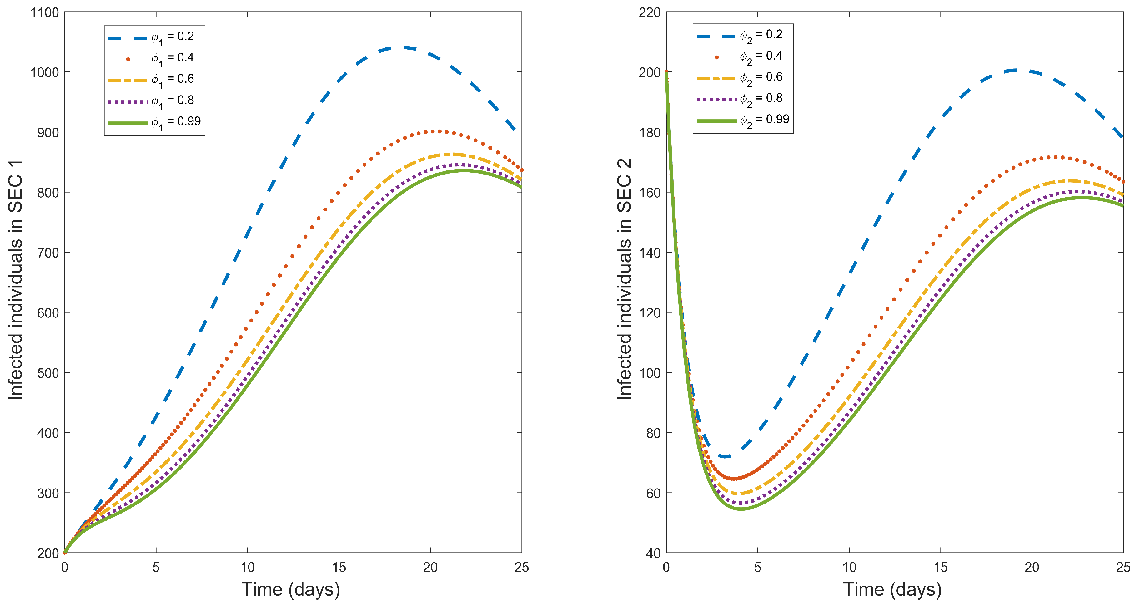
Vaccination is one of the most effective control measures for minimizing typhoid fever [1]. Figure 1 illustrates the influence of vaccination rate in the population. We observe from the figure that increasing vaccination rates leads to a decrease in infected humans in both socio-economic classes. We observe that the infected populace is greater in the lower SEC 1 group in the presence of vaccination. Hence, to achieve disease eradication, this lower SEC 1 group should be the main target of vaccination.

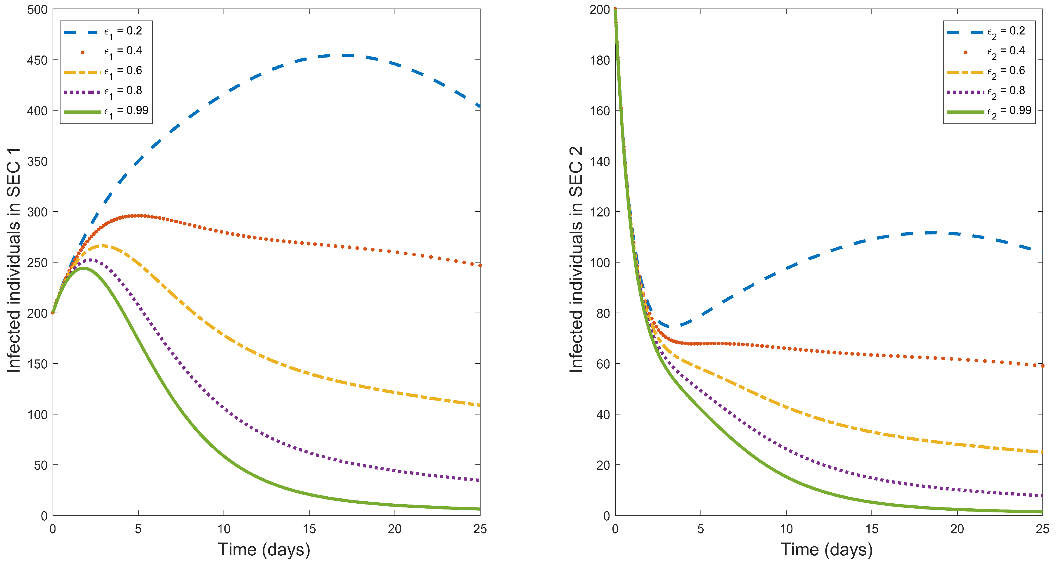
Vaccine efficacy is a major factor in vaccination that determines the percentage reduction of the disease in a vaccinated group. Figure 2 illustrates the impact of vaccine efficacy ${\epsilon }_i$ on the dynamics of typhoid fever. The figure shows that an increase in vaccine efficacy decreases typhoid fever-infected humans in the entire community. Hence, considering a vaccination with a very high efficacy (say 99% as we have in Figure 2) will results in faster disease eradication in the two socio-economic classes if the vaccine is applied uniformly in the entire populace.

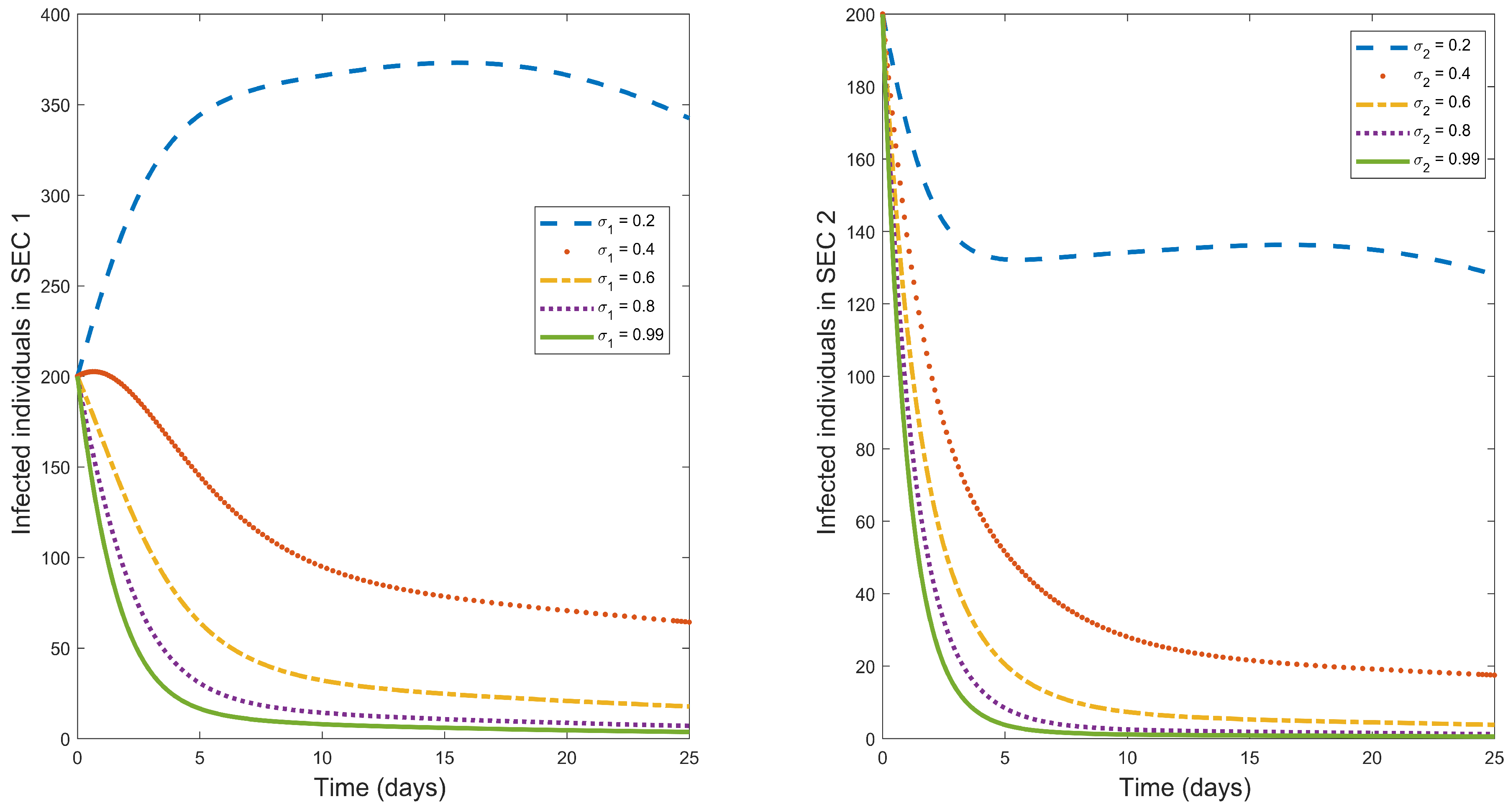
Typhoid fever can be treated with appropriate antibiotic medicine [1]. The treatment of infected individuals is an effective control measure for reducing typhoid fever infections. Figure 3 presents a graphical illustration of the effect of treatment rate in decreasing the spread of typhoid fever.The illustration shows that increasing the treatment rate results in a decrease in typhoid fever in both socio-economic classes. Based on this, effective treatment of infected humans is recommended in the entire population.

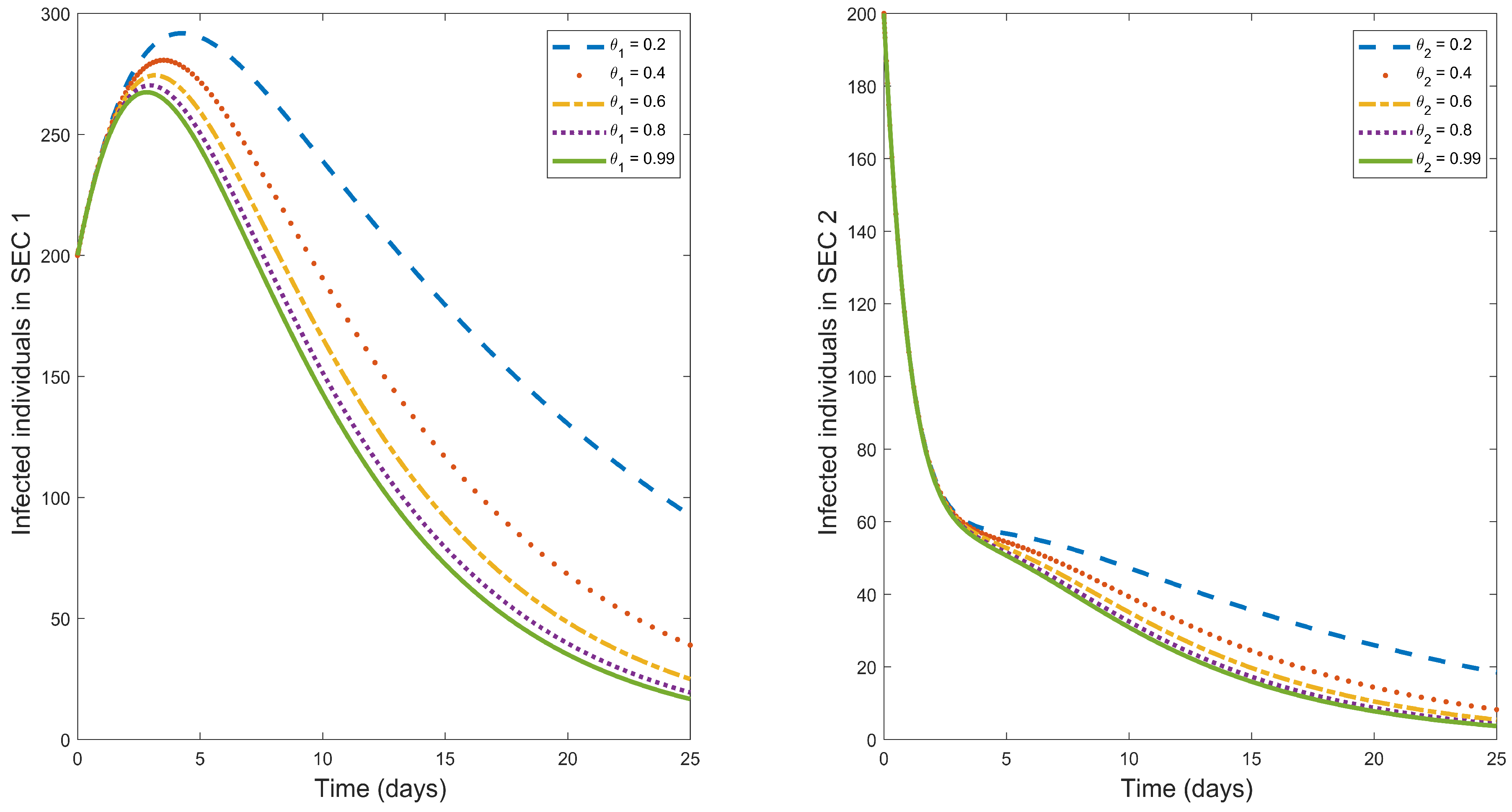
Contaminated food and environment are two of the major routes of contracting typhoid fever [1]. So, to reduce typhoid fever infections, sanitation should be maintained in society. Figure 4 presents a graphical representation of the impact of sanitation ${\theta }_i$ on the dynamics of typhoid fever. From the figure, we observe that an increase in sanitation results in a decrease in typhoid fever-infected humans. The effects of sanitation are less in the higher SEC 2 group. A possible explanation for this could be because the higher SEC 2 group already has a certain level of sanitation in the environment, so introducing what is already in existence in their environment will not lead to major results unlike in the lower SEC 1 group that have limited access to sanitation. Based on these results, the lower SEC 1 group should be the target of sanitation for maximum results.

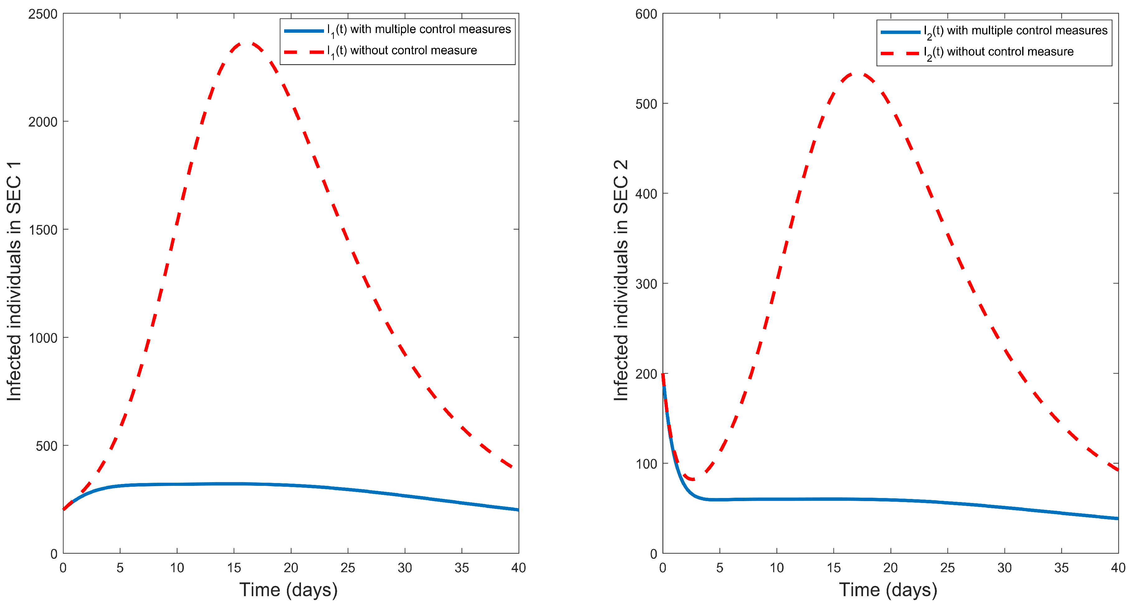
Multiple control measures in this study include the situation when different possible control measures are introduced simultaneously in fighting a particular disease. In this study, we have discussed three possible control measures that can be used in fighting typhoid fever outbreaks. Figure 5 describes the effects of introducing these three control measures in combating typhoid fever. The figure shows that using multiple control measures has maximum influence in decreasing the infected population (in both socio-economic classes) when compared with no control measures. Therefore, whenever a typhoid fever outbreak occurs, multiple control measures should be considered for the fastest eradication of the disease.

5. Optimal Control Analysis

Qualitative and numerical analysis of our model showed that implementing multiple control measures as previously mentioned plays a major role in reducing the influence of typhoid fever. Here, we intend to perform optimal control analysis to determine the most effective control strategy for minimizing the number of humans affected by typhoid fever among different socio-economic classes. To minimize the cost of implementing the controls, we assume that the control parameters ${\varphi }_i$, ${\sigma }_i$ and ${\theta }_i$ denoting vaccination, treatment and sanitation, respectively, are measurable functions of time and then we formulate an appropriate optimal control function that minimizes the cost of implementing the controls subject to the model (1). For simplicity, we write the control strategies as control functions given as ${\varphi }_i=u_i\left(t\right)$, ${\sigma }_i=v_i\left(t\right)$ and ${\theta }_i=w_i$ which are bounded, Lebesgue integral functions. Given the above, we now write the optimal control model as

$$\left\{\begin{array}{c}\frac{d{S}_1\left(t\right)}{dt}=N_1\left(t\right){\mu }_1-({\beta }_1{I}_1\left(t\right)+{\alpha }_1{P}_1\left(t\right))S_1\left(t\right)-({\mu }_1+u_1)S_1\left(t\right)\hfill \\ +{\phi }_1{R}_1\left(t\right)-k_{12}{S}_1\left(t\right)+k_{21}{S}_2\left(t\right),\hfill \\ \frac{d{V}_1\left(t\right)}{dt}=u_1{S}_1\left(t\right)-(1-{\epsilon }_1)({\beta }_1{I}_1\left(t\right)+{\alpha }_1{P}_1\left(t\right))V_1\left(t\right)-{\mu }_1{V}_1\left(t\right),\hfill \\ \frac{d{I}_1\left(t\right)}{dt}=({\beta }_1{I}_1\left(t\right)+{\alpha }_1{P}_1\left(t\right))S_1\left(t\right)+(1-{\epsilon }_1)({\beta }_1{I}_1\left(t\right)+{\alpha }_1{P}_1\left(t\right))V_1\left(t\right)\hfill \\ -({\mu }_1+{\gamma }_1+v_1)I_1\left(t\right)-b_{12}{I}_1\left(t\right)+b_{21}{I}_2\left(t\right),\hfill \\ \frac{d{T}_1\left(t\right)}{dt}=v_1{I}_1\left(t\right)-({\mu }_1+{\rho }_1)T_1\left(t\right),\hfill \\ \frac{d{R}_1\left(t\right)}{dt}={\gamma }_1{I}_1\left(t\right)+{\rho }_1{T}_1\left(t\right)-({\mu }_1+{\phi }_1)R_1\left(t\right),\hfill \\ \frac{d{P}_1\left(t\right)}{dt}={\delta }_1{I}_1\left(t\right)-(\xi +w_1)P_1\left(t\right),\hfill \\ \frac{d{S}_2\left(t\right)}{dt}=N_2\left(t\right){\mu }_2-({\beta }_2{I}_2\left(t\right)+{\alpha }_2{P}_2\left(t\right))S_2\left(t\right)-({\mu }_2+u_2)S_2\left(t\right)\hfill \\ +{\phi }_2{R}_2\left(t\right)+k_{12}{S}_1\left(t\right)-k_{21}{S}_2\left(t\right),\hfill \\ \frac{d{V}_2\left(t\right)}{dt}=u_2{S}_2\left(t\right)-(1-{\epsilon }_2)({\beta }_2{I}_2\left(t\right)+{\alpha }_2{P}_2\left(t\right))V_2\left(t\right)-{\mu }_2{V}_2\left(t\right),\hfill \\ \frac{d{I}_2\left(t\right)}{dt}=({\beta }_2{I}_2\left(t\right)+{\alpha }_2{P}_2\left(t\right))S_2\left(t\right)+(1-{\epsilon }_2)({\beta }_2{I}_2\left(t\right)+{\alpha }_2{P}_2\left(t\right))V_2\left(t\right)\hfill \\ -({\mu }_2+{\gamma }_2+v_2)I_2\left(t\right)+b_{12}{I}_1\left(t\right)-b_{21}{I}_2\left(t\right),\hfill \\ \frac{d{T}_2\left(t\right)}{dt}=v_2{I}_2\left(t\right)-({\mu }_2+{\rho }_2)T_2\left(t\right),\hfill \\ \frac{d{R}_2\left(t\right)}{dt}={\gamma }_2{I}_2\left(t\right)+{\rho }_2{T}_2\left(t\right)-({\mu }_2+{\phi }_2)R_2\left(t\right),\hfill \\ \frac{d{P}_2\left(t\right)}{dt}={\delta }_2{I}_2\left(t\right)-(\xi +w_2)P_2\left(t\right),\hfill \end{array}\right.$$

(5)

subject to the initial conditions $S_1\left(0\right)=S_1^0$, $V_1\left(0\right)=V_1^0$, $I_1=I_1^0$, $T_1\left(0\right)=T_1^0$, $R_1\left(0\right)=R_1^0$, $S_2\left(0\right)=S_2^0$, $V_2\left(0\right)=V_2^0$, $I_2\left(0\right)=I_2^0$, $T_2\left(0\right)=T_2^0$, $R_2\left(0\right)=R_2^0$. This implies that the optimal control model is said to be optimal if it minimizes the objective functional

$$\mathcal{J}(u_i,v_i,w_i)={\int }_0^T\sum _{i=1}^2\{A_i{S}_1+B_i{I}_i+C_i{P}_i+d_i{u}_i^2+e_i{v}_i^2+f_i{w}_i^2\}dt,$$

(6)

subject to the model (5), where the coefficients $A_i$, $B_i$, $C_i$, $d_i$, $e_i$ and $f_i$ are cost balancing coefficients that transform the integral into money expended over time T. Here, $A_i$, is the direct cost associated with reducing the amount of susceptibility to disease in each SEC, $B_i$ is the direct cost associated with reducing the number of infected humans in each SEC and $C_i$ is the direct cost associated with reducing the number of bacteria in the environment, while $d_i$, $e_i$ and $f_i$ are relative costs for enforcing the control strategies $u_i$, $v_i$, $w_i$. The goal is to minimize the number of humans susceptible to typhoid fever among different SECs, minimize the number of infectious humans in all SECs and minimize the bacteria that causes typhoid. In doing this, we anticipate nonlinear costs arising from these controls and so we consider quadratic functions for measuring the control costs [19,31,32,33,34,35].

The goal is to determine an optimal control $u_i$, $v_i$ and $w_i$ such that

$$\mathcal{J}(u_1,v_i,w_i)=\underset{\mathsf{\Omega }}{min}\mathcal{J}(u_1,v_i,w_i),$$

(7)

where $\mathsf{\Omega }=u_i\left(t\right),w_i\left(t\right),w_i\left(t\right)|0\le u_i\left(t\right),v_i\left(t\right),w_i\left(t\right)\le 1$ are measurable.

The Pontryagins Maximum Principle [36] introduces adjoint functions that gives us the opportunity to combine the state system with the objective functional. With the Pontryagins principle we can convert the problem of minimizing the objective functional to the state system into a problem that involves minimizing a Hamiltonian H, with respect to $u_i\left(t\right)$, $v_i\left(t\right)$ and $w_i\left(t\right)$. From the idea above, we now have the Hamiltonian for the objective functional and the state system given as

$$\begin{array}{ccc}\hfill H& =& A_1{S}_1\left(t\right)+B_1{I}_1\left(t\right)+C_1{P}_1\left(t\right)+d_1{u}_1^2\left(t\right)+e_1{v}_1^2\left(t\right)+f_1{w}_1^2\left(t\right)\hfill \\ \hfill & +& {\lambda }_{S_1}({\mu }_1{N}_1\left(t\right)-({\beta }_1{I}_1\left(t\right)+{\alpha }_1{P}_1\left(t\right))S_1\left(t\right)-({\mu }_1+u_1)S_1\left(t\right)+{\phi }_1{R}_1\left(t\right)\hfill \\ \hfill & -& k_{12}{S}_1\left(t\right)+k_{21}{S}_2\left(t\right))+{\lambda }_{V_1}(u_1{S}_1\left(t\right)-(1-{ϵ}_1)({\beta }_1{I}_1\left(t\right)+{\alpha }_1{P}_1\left(t\right))V_1\left(t\right)-{\mu }_1{V}_1\left(t\right))\hfill \\ \hfill & +& {\lambda }_{I_1}(({\beta }_1{I}_1\left(t\right)+{\alpha }_1{P}_1\left(t\right))S_1\left(t\right)+(1-ϵ)({\beta }_1{I}_1\left(t\right)+{\alpha }_1{P}_1\left(t\right))V_1\left(t\right)\hfill \\ \hfill & -& ({\mu }_1+{\gamma }_1+{\nu }_1)I_1\left(t\right)-b_{12}I\left(t\right)+b_{21}{I}_2\left(t\right))+{\lambda }_{T_1}({\nu }_1{I}_1\left(t\right)-({\mu }_1+{\rho }_1)T_1\left(t\right))\hfill \\ \hfill & +& {\lambda }_{R_1}({\gamma }_1{I}_1\left(t\right)+{\rho }_1{T}_1\left(t\right)-({\mu }_1+{\phi }_1)R_1\left(t\right))+{\lambda }_{P_1}({\delta }_1{I}_1\left(t\right)-({\xi }_1+w_1)P_1\left(t\right))\hfill \\ \hfill & +& A_2{S}_2\left(t\right)+B_2{I}_2\left(t\right)+C_2{P}_2\left(t\right)+d_2{u}_2^2\left(t\right)+e_2{v}_2^2\left(t\right)+f_2{w}_2^2\left(t\right)\hfill \\ \hfill & +& {\lambda }_{S_2}({\mu }_2{N}_2\left(t\right)-({\beta }_2{I}_2\left(t\right)+{\alpha }_2{P}_2\left(t\right))S_2\left(t\right)-({\mu }_2+u_2)S_2\left(t\right)+{\phi }_2{R}_2\left(t\right)+k_{12}{S}_1\left(t\right)\hfill \\ \hfill & -& k_{21}{S}_2\left(t\right))+{\lambda }_{V_2}(u_2{S}_2\left(t\right)-(1-{ϵ}_2)({\beta }_2{I}_2\left(t\right)+{\alpha }_2{P}_2\left(t\right))V_2\left(t\right)-{\mu }_2{V}_2\left(t\right))\hfill \\ \hfill & +& {\lambda }_{I_2}(({\beta }_2{I}_2\left(t\right)+{\alpha }_2{P}_2\left(t\right))S_2\left(t\right)+(1-ϵ)({\beta }_2{I}_1\left(t\right)+{\alpha }_2{P}_2\left(t\right))V_2\left(t\right)-({\mu }_2+{\gamma }_2+{\nu }_2)I_2\left(t\right)\hfill \\ \hfill & +& b_{12}I\left(t\right)-b_{21}{I}_2\left(t\right))+{\lambda }_{T_2}({\nu }_2{I}_2\left(t\right)-({\mu }_2+{\rho }_2)T_2\left(t\right))\hfill \\ \hfill & +& {\lambda }_{R_2}({\gamma }_2{I}_2\left(t\right)+{\rho }_2{T}_2\left(t\right)-({\mu }_2+{\phi }_2)R_2\left(t\right))+{\lambda }_{P_2}({\delta }_2{I}_2\left(t\right)-({\xi }_2+w_2)P_2\left(t\right)),\hfill \end{array}$$

where ${\lambda }_{S1}$, ${\lambda }_{V1}$, ${\lambda }_{I1}$, ${\lambda }_{T1}$, ${\lambda }_{R1}$, ${\lambda }_{P1}$, ${\lambda }_{S2}$, ${\lambda }_{V2}$, ${\lambda }_{I2}$, ${\lambda }_{T2}$, ${\lambda }_{R2}$, and ${\lambda }_{P2}$ are associated adjoint for the states $S_i$, $V_i$, $I_i$, $T_i$, $R_i$ and $P_i$, respectively. Given an optimal control triple ($u_i^{*}\left(t\right)$, $v_i^{*}\left(t\right)$, $w_i^{*}\left(t\right)$) together with corresponding states ($S_i^{*}$, $V_i^{*}$, $I_i^{*}$, $T_i^{*}$, $R_i^{*}$, $P_i^{*}$) that minimizes $\mathcal{J}(u_i,v_i,w_i)$ over $\mathsf{\Omega }$, there exist adjoint variables ${\lambda }_{Si}$, ${\lambda }_{Vi}$, ${\lambda }_{Ii}$, ${\lambda }_{Ti}$, ${\lambda }_{Ri}$, and ${\lambda }_{Pi}$$(i=1,2)$ that satisfy

$$\begin{array}{ccc}\hfill \frac{d{\lambda }_{S_1}}{dt}& =& -A_1+{\lambda }_{S_1}({\beta }_1{I}_1\left(t\right)+{\alpha }_1{P}_1\left(t\right)+({\mu }_1+u_1)-k_{12})-{\lambda }_{V_1}{u}_1-{\lambda }_{I_1}({\beta }_1{I}_1+{\alpha }_1{P}_1\left(t\right)),\hfill \\ \hfill \frac{d{\lambda }_{V_1}}{dt}& =& {\lambda }_{V_1}((1-{ϵ}_1)({\beta }_1{I}_1\left(t\right)+{\alpha }_1{P}_1\left(t\right))+{\mu }_1)-{\lambda }_{I_1}\left((1-{ϵ}_1)({\beta }_1{I}_1\left(t\right)+{\alpha }_1{P}_1\left(t\right))\right),\hfill \\ \hfill \frac{d{\lambda }_{I_1}}{dt}& =& -B_1+{\lambda }_{S_1}{\beta }_1{S}_1\left(t\right)+{\lambda }_{V_1}(1-{ϵ}_1){\beta }_1{V}_1\left(t\right)-{\lambda }_{I_1}({\beta }_1{S}_1\left(t\right)+(1-{ϵ}_1){\beta }_1{V}_1\left(t\right)\hfill \\ \hfill & -& ({\mu }_1+{\gamma }_1+{\nu }_1)-b_{12})-{\lambda }_{T_1}{v}_1-{\lambda }_{R_1}{\gamma }_1-{\lambda }_{P_1}{\delta }_1,\hfill \\ \hfill \frac{d{\lambda }_{T_1}}{dt}& =& {\lambda }_{T_1}({\mu }_1+{\rho }_1)-{\lambda }_{R_1}{\rho }_1,\hfill \\ \hfill \frac{d{\lambda }_{R_1}}{dt}& =& -{\lambda }_{S_1}{\phi }_1+{\lambda }_{R_1}({\mu }_1+{\phi }_1),\hfill \\ \hfill \frac{d{\lambda }_{P_1}}{dt}& =& -C_1+{\lambda }_{S_1}{\alpha }_1{S}_1\left(t\right)+{\lambda }_{V_1}(1-{ϵ}_1){\alpha }_1{V}_1\left(t\right)-{\lambda }_{I_1}{\alpha }_1(S_1\left(t\right)+(1-{ϵ}_1)V_1\left(t\right))\hfill \\ \hfill & +& {\lambda }_{P_1}({\xi }_1+w_1),\hfill \\ \hfill \end{array}$$

$$\begin{array}{ccc}\hfill \frac{d{\lambda }_{S_2}}{dt}& =& -A_2+{\lambda }_{S_2}({\beta }_2{I}_2\left(t\right)+{\alpha }_2{P}_2\left(t\right)+({\mu }_2+u_2)+k_{21})-{\lambda }_{V_2}{u}_2-{\lambda }_{I_2}({\beta }_2{I}_2+{\alpha }_2{P}_2\left(t\right)),\hfill \\ \hfill \frac{d{\lambda }_{V_2}}{dt}& =& {\lambda }_{V_2}((1-{ϵ}_2)({\beta }_2{I}_2\left(t\right)+{\alpha }_2{P}_2\left(t\right))+{\mu }_2)-{\lambda }_{I_2}(1-{ϵ}_2)({\beta }_2{I}_2\left(t\right)+{\alpha }_2{P}_2\left(t\right)),\hfill \\ \hfill \frac{d{\lambda }_{I_2}}{dt}& =& -B_2+{\lambda }_{S_2}{\beta }_2{S}_2\left(t\right)+{\lambda }_{V_2}(1-{ϵ}_2){\beta }_2{V}_2\left(t\right)-{\lambda }_{I_2}({\beta }_2{S}_2\left(t\right)+(1-{ϵ}_2){\beta }_2{V}_2\left(t\right)\hfill \\ \hfill & -& ({\mu }_2+{\gamma }_2+{\nu }_2)+b_{21})-{\lambda }_{T_2}{v}_2-{\lambda }_{R_2}{\gamma }_2-{\lambda }_{P_2}{\delta }_2,\hfill \\ \hfill \frac{d{\lambda }_{T_2}}{dt}& =& {\lambda }_{T_2}({\mu }_2+{\rho }_2)-{\lambda }_{R_2}{\rho }_2,\hfill \\ \hfill \frac{d{\lambda }_{R_2}}{dt}& =& -{\lambda }_{S_2}{\phi }_2+{\lambda }_{R_2}({\mu }_2+{\phi }_2),\hfill \\ \hfill \frac{d{\lambda }_{P_2}}{dt}& =& -C_2+{\lambda }_{S_2}{\alpha }_2{S}_2\left(t\right)+{\lambda }_{V_2}(1-{ϵ}_2){\alpha }_2{V}_2\left(t\right)-{\lambda }_{I_2}{\alpha }_2\left(S_2\left(t\right)+(1-{ϵ}_2{V}_2\left(t\right)\right)\hfill \\ \hfill & +& {\lambda }_{P_2}({\xi }_2+w_2),\hfill \end{array}$$

(8)

together with the transversality conditions ${\lambda }_k\left(t_f\right)=0$, for $k=S_i,V_i,I_i,T_i,R_i$ and $P_i$.

Note that we obtain the differential Equation (8) which governs the adjoint variables by differentiating the appropriate Hamiltonian function (8) with respect to the corresponding state as follows:

$$\frac{d{\lambda }_k}{dt}=\frac{dH}{dk}.$$

(9)

Now, consider the optimality conditions

$$\begin{array}{c}\hfill \frac{\partial H}{\partial u_i}=0,\frac{\partial H}{\partial v_i}=0,\frac{\partial H}{\partial w_i}=0.\end{array}$$

(10)

So for the control triplet $u_i^{*}$, $v_i^{*}$ and $w_i^{*}$ to satisfy the optimality condition we have;

For $u_i$ we have

$$2d_i{u}_i^{*}-{\lambda }_{S_i}{S}_i\left(t\right)+{\lambda }_{V_i}{S}_i\left(t\right)=0.$$

(11)

The solving for $u_i$ using the optimality condition (10), we have

$$u_i^{*}=\frac{S_i\left(t\right)({\lambda }_{S_i}-{\lambda }_{V_i})}{2d_i},$$

(12)

and subsequently taking bounds into consideration, we have

$$u_i^{*}=min\left(1,max\left(0,\frac{S_i\left(t\right)({\lambda }_{S_i}-{\lambda }_{V_i})}{2d_i}\right)\right).$$

(13)

Solving for $v_i$ using the optimality condition, we have

$$v_i^{*}=\frac{I_i\left(t\right)({\lambda }_{I_i}-{\lambda }_{T_i})}{2e_i},$$

(14)

and subsequently taking bounds into consideration, we have

$$v_i^{*}=min\left(1,max\left(0,\frac{I_i\left(t\right)({\lambda }_{I_i}-{\lambda }_{T_i})}{2e_i}\right)\right).$$

(15)

Similarly for $w_i$, we have

$$w_i^{*}=min\left(1,max\left(0,\frac{{\lambda }_{P_i}{P}_i\left(t\right)}{2f_i}\right)\right),(i=1,2).$$

(16)

The results obtained above shows that the optimal triple $(u_i^{*},v_i^{*},w_i^{*})$ has the ability to minimize the impact of typhoid fever in any human population, if the control measures of the disease are applied at a minimum cost. To determine the explicit effect of the optimal control parameters and how they influence the eradication of typhoid fever, further analysis will be carried since the optimal control triple is parameter-dependent. The extent of the optimal control parameters reducing the disease can also be investigated with reference to the implicated cost. To provide an illustration of how these parameters may affect the reduction of typhoid fever, we use data from related literature from peer-reviewed publications and carry out a numerical simulation to give a visual view of our results.

5.1. Existence of the Optimal Control

Let $x=(u_i,v_i,w_i)\in {\left[L^2(0,T)\right]}^3$ and $\mathcal{I}=(S_i,I_i,P_i)$. Hence, a reduced function corresponding to (6) is given by

$$\mathcal{J}(x,I^x)={\int }_0^T\sum _{i=1}^2\left\{A_i{S}_i+B_i{I}_i+C_i{P}_i+d_i{u}_i^2+e_i{v}_i^2+f_i{w}_i^2\right\}dt,x\in \mathsf{\Omega }.$$

(17)

Set $\mathsf{\Omega }$ is convex and closed.

Proof. 

To prove that $\mathsf{\Omega }$ is a closed set, assume that $x_{m\in \mathbb{N}}⟶x^{*}$ in $L^2(0,T)$ for $x_m\in \mathsf{\Omega }$ but $x^{*}\notin \mathsf{\Omega }$, i.e., $x^{*}<0$ or $x^{*}>1$ on a set of positive measure. Then taking $x^{*}<0$, from Lebesgue measure methods there exists $ϵ>0$ and a positive measure set $(0,t)\subset (0,T)$ such that $x^{*}\le 0-ϵ$ on $(0,t)$ [37]. This implies that

$${\int }_0^T{(x_m-x^{*})}^{2}dt\ge {\int }_0^t{(x_m-x^{*})}^{2}dt\ge {\int }_0^t{(0-x^{*})}^{2}dt\ge {\int }_0^t{ϵ}^{2}dt>0,$$

a contradiction. Thus, set $\mathsf{\Omega }$ is closed and an analogous proof also holds for $x^{*}<1$.

To prove convexity of set $\mathsf{\Omega }$, it suffices to show that if $\mathsf{\Omega }$ is a convex set and $u_i,v_i,w_i\in \mathsf{\Omega }$, then any convex combination of any of $u_i,v_i,w_i$ (say $u_i$) ${\sum }_{i=1}^2{\varphi }_i{u}_i$ for ${\sum }_{i=1}^2{\varphi }_i=1$, ${\varphi }_1,{\varphi }_2\ge 0$ is also contained in $\mathsf{\Omega }$.

The proof is by induction. For $i=1$, since $u_1\in \mathsf{\Omega }$ then ${\varphi }_1{u}_1\in \mathsf{\Omega }$. For $i=2$, since $(u_1,u_2)\in \mathsf{\Omega }$,

$$0\le u_1\le 1,$$

(18)

and

$$0\le u_2\le 1.$$

(19)

Multiplying (18) by ${\varphi }_1$ and (19) by ${\varphi }_2$ gives

$$0\le {\varphi }_1{u}_1\le {\varphi }_1,$$

(20)

and

$$0\le {\varphi }_2{u}_2\le {\varphi }_2.$$

(21)

Adding up Equations (20) and (21), we have

$$0\le {\varphi }_1{u}_1+{\varphi }_2{u}_2\le 1.$$

Thus, ${\varphi }_1{u}_1+{\varphi }_2{u}_2\in \mathsf{\Omega }$. This also relates to $v_1,v_2$ and $w_1,w_2$. This can also be extended to the n-th socio-economic class.

For $i=n-1$, suppose that ${\sum }_{i=1}^{n-1}{\varphi }_i{u}_i\in \mathsf{\Omega }$. By the inductive hypothesis,

$$y=\frac{{\varphi }_1{u}_1}{{\sum }_{i=1}^{n-1}{\varphi }_i}+\frac{{\varphi }_2{u}_2}{{\sum }_{i=1}^{n-1}{\varphi }_1}+\dots +\frac{{\varphi }_{n-1}{u}_{n-1}}{{\sum }_{i=1}^{n-1}{\varphi }_i}\in \mathsf{\Omega }.$$

(22)

For $i=n$,

$$\sum _{i=1}^n{\varphi }_i{u}_i=\sum _{i=1}^{n-1}{\varphi }_i{u}_i+{\varphi }_n{u}_n.$$

(23)

From (22), ${\sum }_{i=1}^{n-1}{\varphi }_i{u}_i=y{\sum }_{i=1}^{n-1}{\varphi }_i$. Then (23) gives

$$\sum _{i=1}^n{\varphi }_i{u}_i=y\sum _{i=1}^{n-1}{\varphi }_i+{\varphi }_n{u}_n.$$

(24)

Since $u_n\in \mathsf{\Omega }$ it follows that the RHS of (24) is a convex combination of two points of $\mathsf{\Omega }$. Thus, $y{\sum }_{i=1}^{n-1}{\varphi }_i+{\varphi }_n{u}_n\in \mathsf{\Omega }$, so, is $y{\sum }_{i=1}^{n-1}{\varphi }_i+{\varphi }_n{v}_n\in \mathsf{\Omega }$ and $y{\sum }_{i=1}^{n-1}{\varphi }_i+{\varphi }_n{w}_n\in \mathsf{\Omega }$ hence, $\mathsf{\Omega }$ is convex. □

There exists an optimal control pair $(x^{*},{\mathcal{I}}^{x^{*}})$ to the optimization problem (7).

Proof. 

Set

$$b=\underset{x\in \mathsf{\Omega }}{sup}\mathcal{J}(x,I^x).$$

This implies, for any $m\in \mathbb{N}$, there exists $x_m\in \mathsf{\Omega }$ so that

$$b-\frac{1}{m}<\mathcal{J}(x_m,{\mathcal{I}}^{x_m})\le b.$$

(25)

As set $\mathsf{\Omega }$ is a bounded subset of $L^2(0,T)$, it follows from Bolzano-Weierstrass theorem, that there exists a subsequence ${\left\{x_{m_r}\right\}}_{r\in \mathbb{N}}$ such that

$$x_{m_r}⟶x^{*},$$

(26)

weakly in $L^2(0,T)$. From (2) we have that all non-negative initial conditions are bounded. Thus, there exists a subsequence ${\left\{{\mathcal{I}}^{x_{mr}}\right\}}_{r\in \mathbb{N}}$ such that

$${\mathcal{I}}^{x_{mr}}⟶{\mathcal{I}}^{x^{*}}\mathrm{in}C\left([0,T]\right).$$

(27)

From (25),

$$b-\frac{1}{m}<{\int }_0^T\sum _{i=1}^2\left\{A_i{S}_i^{u_{imr}}\left(t\right)+B_i{I}_i^{v_{imr}}\left(t\right)+C_i{P}_i^{w_{imr}}\left(t\right)+d_i{u}_{i_{mr}}^2+e_i{v}_{i_{mr}}^2+f_i{w}_{i_{mr}}^2\right\}dt\le b.$$

(28)

By (25) and (27), passing to the limit in (30),

$$b={\int }_0^T\sum _{i=1}^2\left\{A_i{S}_i^{u_i^{*}}\left(t\right)+B_i{I}_i^{v_i^{*}}\left(t\right)+C_i{P}_i^{w_i^{*}}\left(t\right)+d_i{\left(u_i^{*}\right)}^2+e_i{\left(v_i^{*}\right)}^2+f_i{\left(w_i^{*}\right)}^2\right\}dt,$$

(29)

that is, $((u_i^{*},v_i^{*},w_i^{*}),(S_i^{u^{*}},I_i^{v^{*}},P_i^{w^{*}}))$, $i=1,2$ is an optimal pair where $u_i^{*}$, $v_i^{*}$ and $w_i^{*}$ are optimal controls for (7). □

5.2. Uniqueness of the Optimal Control System

The optimality system of our optimal control problem is the combination of model (5) and the adjoint variables (8). So we have

$$\begin{array}{ccc}\hfill \frac{d{S}_i\left(t\right)}{dt}& =& N_i\left(t\right){\mu }_i-({\beta }_i{I}_i\left(t\right)+{\alpha }_i{P}_i\left(t\right))S_i\left(t\right)-({\mu }_i+u_i)S_i\left(t\right)+{\phi }_i{R}_i\left(t\right)-k_{i,j}{S}_i\left(t\right)+k_{j,i}{S}_j\left(t\right),\hfill \\ \hfill \frac{d{V}_i\left(t\right)}{dt}& =& u_i{S}_i\left(t\right)-(1-{\epsilon }_i)({\beta }_i{I}_i\left(t\right)+{\alpha }_i{P}_i\left(t\right))V_i\left(t\right)-{\mu }_i{V}_i\left(t\right),\hfill \\ \hfill \frac{d{I}_i\left(t\right)}{dt}& =& ({\beta }_i{I}_i\left(t\right)+{\alpha }_i{P}_i\left(t\right))S_i\left(t\right)+(1-{\epsilon }_i)({\beta }_i{I}_i\left(t\right)+{\alpha }_i{P}_i\left(t\right))V_i\left(t\right)-({\mu }_i+{\gamma }_i+v_i)I_i\left(t\right)\hfill \\ \hfill & -& b_{i,j}{I}_i\left(t\right)+b_{j,i}{I}_j\left(t\right),\hfill \\ \hfill \frac{d{T}_i\left(t\right)}{dt}& =& v_i{I}_i\left(t\right)-({\mu }_i+{\rho }_i)T_i\left(t\right),\hfill \\ \hfill \frac{d{R}_i\left(t\right)}{dt}& =& {\gamma }_i{I}_i\left(t\right)+{\rho }_i{T}_i\left(t\right)-({\mu }_i+{\phi }_i)R_i\left(t\right),\hfill \\ \hfill \frac{d{P}_i\left(t\right)}{dt}& =& {\delta }_i{I}_i\left(t\right)-({\xi }_i+w_i)P_i\left(t\right),\hfill \\ \hfill \frac{d{\lambda }_{S_i}}{dt}& =& -A_i+{\lambda }_{S_i}({\alpha }_i{P}_i\left(t\right)+({\mu }_i+u_i)-k_{ij})-{\lambda }_{V_i}{u}_i+{\lambda }_{I_i}{\alpha }_i{P}_i\left(t\right),\hfill \\ \hfill \frac{d{\lambda }_{V_i}}{dt}& =& {\lambda }_{V_i}((1-{ϵ}_i)({\beta }_i{I}_i\left(t\right)+{\alpha }_i{P}_i\left(t\right))+{\mu }_i)-{\lambda }_{I_i}(1-{ϵ}_i)({\beta }_i{I}_i\left(t\right)+{\alpha }_i{P}_i\left(t\right)),\hfill \\ \hfill \frac{d{\lambda }_{I_i}}{dt}& =& -B_i-{\lambda }_{I_i}({\beta }_i{S}_i\left(t\right)+(1-{ϵ}_i){\beta }_i{V}_i\left(t\right)-({\mu }_i+{\gamma }_i+{\nu }_i)-b_{ij})-{\lambda }_{I_i}{V}_i\left(t\right)\hfill \\ \hfill & -& {\lambda }_{R_i}{\gamma }_i-{\lambda }_{P_i}{\delta }_i,\hfill \\ \hfill \frac{d{\lambda }_{T_i}}{dt}& =& {\lambda }_{T_i}({\mu }_i+{\rho }_i)-{\lambda }_{R_i}{\rho }_i,\hfill \\ \hfill \frac{d{\lambda }_{R_i}}{dt}& =& -{\phi }_i+{\lambda }_{R_i}({\mu }_i+{\phi }_i),\hfill \\ \hfill \frac{d{\lambda }_{P_i}}{dt}& =& -C_i+{\lambda }_{S_i}{\alpha }_i{S}_i\left(t\right)+(1-{ϵ}_i){\alpha }_i{V}_i\left(t\right)+{\lambda }_{I_i}{\alpha }_i{S}_i\left(t\right)-(1-{ϵ}_i){\alpha }_i{V}_i\left(t\right)+{\lambda }_{P_i}({\xi }_i+w_i),\hfill \end{array}$$

(30)

where $S_i\left(t_0\right)$, $I_i\left(t_0\right)$, $P_i\left(t_0\right)\ge 0$, and ${\lambda }_{S_i}=0$, ${\lambda }_{V_i}=0$, ${\lambda }_{I_i}=0$, ${\lambda }_{T_i}=0$, ${\lambda }_{R_i}=0$, ${\lambda }_{P_i}=0$.

For sufficiently small $t_f$, the solution to the optimality system (30) of the optimal control problem is unique.

Proof. 

Suppose $(S_i,V_i,I_i,T_i,R_i,P_i,{\lambda }_{S_i},{\lambda }_{V_i},{\lambda }_{I_i},{\lambda }_{T_i},{\lambda }_{R_i},{\lambda }_{R_i})$, and $({\tilde{S}}_i,{\tilde{V}}_i,{\tilde{I}}_i,{\tilde{T}}_i,{\tilde{R}}_i,{\tilde{P}}_i,{\tilde{\lambda }}_{S_i},{\tilde{\lambda }}_{V_i},{\tilde{\lambda }}_{I_i},{\tilde{\lambda }}_{T_i},{\tilde{\lambda }}_{R_i},{\tilde{\lambda }}_{R_i})$ are two solutions of the optimality system (30). Let $S_i=e^{\lambda it}{x}_1$, $V_i=e^{\lambda it}{x}_2$, $I_i=e^{\lambda it}{x}_3$, $T_i=e^{\lambda it}{x}_4$, $R_i=e^{\lambda it}{x}_5$, $P_i=e^{\lambda it}{x}_6$, ${\lambda }_{S_i}=e^{-\lambda it}{y}_1$, ${\lambda }_{V_i}=e^{-\lambda it}{y}_2$, ${\lambda }_{I_i}=e^{-\lambda it}{y}_3$, ${\lambda }_{T_i}=e^{-\lambda it}{y}_4$, ${\lambda }_{R_i}=e^{-\lambda it}{y}_5$, ${\lambda }_{P_i}=e^{-\lambda it}{y}_6$, ${\tilde{S}}_i=e^{\lambda it}{\tilde{x}}_1$, ${\tilde{V}}_i=e^{\lambda it}{\tilde{x}}_2$, ${\tilde{I}}_i=e^{\lambda it}{\tilde{x}}_3$, ${\tilde{T}}_i=e^{\lambda it}{\tilde{x}}_4$, ${\tilde{R}}_i=e^{\lambda it}{\tilde{x}}_5$, ${\tilde{P}}_i=e^{\lambda it}{\tilde{x}}_6$, ${\tilde{\lambda }}_{S_i}=e^{-\lambda it}{\tilde{y}}_1$, ${\tilde{\lambda }}_{V_i}=e^{-\lambda it}{\tilde{y}}_2$, ${\tilde{\lambda }}_{I_i}=e^{-\lambda it}{\tilde{y}}_3$, ${\tilde{\lambda }}_{T_i}=e^{-\lambda it}{\tilde{y}}_4$, ${\tilde{\lambda }}_{R_i}=e^{-\lambda it}{\tilde{y}}_5$, ${\tilde{\lambda }}_{P_i}=e^{-\lambda it}{\tilde{y}}_6$, where $\lambda$ is chosen arbitrarily. We now let

$$\begin{array}{ccc}\hfill u_i^{*}& =& min\left(1,max\left(0,\frac{x_1(y_1-y_2)}{2d_i}\right)\right),\hfill \\ \hfill v_i^{*}& =& min\left(1,max\left(0,\frac{x_3(y_3-y_4)}{2e_i}\right)\right),\hfill \\ \hfill w_i^{*}& =& min\left(1,max\left(0,\frac{y_6{x}_6}{2f_i}\right)\right),\hfill \\ \hfill {\tilde{u}}_i^{*}& =& min\left(1,max\left(0,\frac{{\tilde{x}}_1({\tilde{y}}_1-{\tilde{y}}_2)}{2d_i}\right)\right),\hfill \\ \hfill {\tilde{v}}_i^{*}& =& min\left(1,max\left(0,\frac{{\tilde{x}}_3({\tilde{y}}_3-{\tilde{y}}_4)}{2e_i}\right)\right),\hfill \\ \hfill {\tilde{w}}_i^{*}& =& min\left(1,max\left(0,\frac{{\tilde{y}}_6{\tilde{x}}_6}{2f_i}\right)\right),(i=1,2)\hfill \end{array}$$

Now let us consider the first Equation of (30), we have

$$\begin{array}{ccc}\hfill {\dot{x}}_1+{\lambda }_i{x}_1& =& {\mu }_i{N}_i{e}^{-\lambda t}-{\beta }_i{x}_3{x}_1-{\alpha }_i{x}_6{x}_1-{\mu }_i{x}_1+{\phi }_i{x}_5-k_{ij}{x}_1+k_{ji}{x}_2,\hfill \\ \hfill {\tilde{\dot{x}}}_1+{\lambda }_i{\tilde{x}}_1& =& {\mu }_i{N}_i{e}^{-\lambda t}-{\beta }_i{\tilde{x}}_3{\tilde{x}}_1-{\alpha }_i{\tilde{x}}_6{\tilde{x}}_1-{\mu }_i{\tilde{x}}_1+{\phi }_i{\tilde{x}}_5-k_{ij}{\tilde{x}}_1+k_{ji}{\tilde{x}}_2.\hfill \end{array}$$

For simplicity, we assume that there is no movement between $S_1$ and $S_2$ in this proof.

By subtracting and integrating from $t_0$ to $t_f$ for the above two equations, we have

$$\begin{array}{ccc}\hfill \frac{1}{2}{(x_1\left(t_f\right)-{\tilde{x}}_1\left(t_f\right))}^2+({\lambda }_i+{\mu }_i){\int }_{t_0}^{t_f}{(x_1-{\tilde{x}}_1)}^{2}dt& =& -{\beta }_i{\int }_{t_0}^{t_f}(x_1{x}_3-{\tilde{x}}_1{\tilde{x}}_3)(x_1-{\tilde{x}}_1)dt\hfill \\ \hfill & -& {\alpha }_i{\int }_{t_0}^{t_f}(x_1{x}_6-{\tilde{x}}_1{\tilde{x}}_6)(x_1-{\tilde{x}}_1)dt\hfill \\ & +& \phi {\int }_{t_0}^{t_f}(x_5-{\tilde{x}}_5)(x_1-{\tilde{x}}_1)dt.\hfill \end{array}$$

(31)

Note that

$$\begin{array}{ccc}\hfill {\int }_{t_0}^{t_f}{(u_i-{\tilde{u}}_i)}^{2}dt& \le & {\left(\frac{1}{2d_i}\right)}^2{\int }_{t_0}^{t_f}{[x_1(y_1-y_2)-{\tilde{x}}_1({\tilde{y}}_1-{\tilde{y}}_2)]}^{2}dt,\hfill \\ \hfill & \le & \left(\frac{1}{2d_i}\right)L_1{\int }_{t_0}^{t_f}[{(x_1-{\tilde{x}}_1)}^2+{(y_1-{\tilde{y}}_1)}^2+{(y_2-{\tilde{y}}_2)}^2]dt,\hfill \\ \hfill {\int }_{t_0}^{t_f}{(v_i-{\tilde{v}}_i)}^{2}dt& \le & {\left(\frac{1}{2e_i}\right)}^2{\int }_{t_0}^{t_f}{[x_3(y_3-y_4)-{\tilde{x}}_3({\tilde{y}}_3-{\tilde{y}}_4)]}^{2}dt,\hfill \\ \hfill & \le & \left(\frac{1}{2e_i}\right)L_2{\int }_{t_0}^{t_f}[{(x_3-{\tilde{x}}_3)}^2+{(y_3-{\tilde{y}}_3)}^2+{(y_4-{\tilde{y}}_4)}^2]dt,\hfill \\ \hfill {\int }_{t_0}^{t_f}{(w_i-{\tilde{w}}_i)}^{2}dt& \le & {\left(\frac{1}{2f_i}\right)}^2{\int }_{t_0}^{t_f}{[x_6{y}_6-{\tilde{x}}_6{\tilde{y}}_6]}^{2}dt,\hfill \\ \hfill & \le & \left(\frac{1}{2f_i}\right)L_3{\int }_{t_0}^{t_f}[{(x_6-{\tilde{x}}_6)}^2+{(y_6-{\tilde{y}}_6)}^2]dt,\hfill \\ \hfill {\int }_{t_0}^{t_f}(x_1{x}_3-{\tilde{x}}_1{\tilde{x}}_3)(x_1-{\tilde{x}}_1)dt& \le & {\int }_{t_0}^{t_f}[{(x_1-{\tilde{x}}_1)}^2{x}_3+{\tilde{x}}_1(x_3-{\tilde{x}}_3)(x_1-{\tilde{x}}_1)]dt,\hfill \\ \hfill & \le & C_1{\int }_{t_0}^{t_f}[{(x_1-{\tilde{x}}_1)}^2+{(x_3-{\tilde{x}}_3)}^2]dt,\hfill \\ \hfill {\int }_{t_0}^{t_f}(x_1{x}_6-{\tilde{x}}_1{\tilde{x}}_6)(x_1-{\tilde{x}}_1)dt& =& {\int }_{t_0}^{t_f}[{(x_1-{\tilde{x}}_1)}^2{x}_6+{\tilde{x}}_1(x_6-{\tilde{x}}_6)(x_1-{\tilde{x}}_1)]dt,\hfill \\ \hfill & \le & C_2{\int }_{t_0}^{t_f}[{(x_1-{\tilde{x}}_1)}^2+{(x_6-{\tilde{x}}_6)}^2]dt,\hfill \\ \hfill {\int }_{t_0}^{t_f}(x_5-{\tilde{x}}_5)(x_1-{\tilde{x}}_1)dt& \le & C_3{\int }_{t_0}^{t_f}(x_5-{\tilde{x}}_5)dt,\hfill \end{array}$$

where $C_1$ depends on the bounds of ${\tilde{x}}_1,x_3$, $C_2$ depends on the bounds of ${\tilde{x}}_1,x_6$, $C_3$ depends on the bounds of $x_5,{\tilde{x}}_5$. So, by (31), we have

$$\begin{array}{ccc}\hfill \frac{1}{2}{(x_1\left(t_f\right)-{\tilde{x}}_1\left(t_f\right))}^2+({\lambda }_i+{\mu }_i){\int }_{t_0}^{t_f}{(x_1-{\tilde{x}}_1)}^{2}dt& \le & M_1{\int }_{t_0}^{t_f}[{(x_1-{\tilde{x}}_1)}^2{(x_3-{\tilde{x}}_3)}^2+{(x_5-{\tilde{x}}_5)}^2+{(x_6-{\tilde{x}}_6)}^2]dt\hfill \\ \hfill & +& N_1{\int }_{t_0}^{t_f}[{(x_1-{\tilde{x}}_1)}^2+{(y_1-{\tilde{y}}_1)}^2\hfill \\ & +& {(y_2-{\tilde{y}}_2)}^2]dt,\hfill \end{array}$$

(32)

where $M_1$ is an appropriate upper-bound. Similarly, we can obtain the following inequalities for $(x_k\left(t_f\right),{\tilde{x}}_k\left(t_f\right))$ and $(y_l\left(t_f\right),{\tilde{y}}_l\left(t_0\right))$$(k=1,2,3,5,6$, $l=1,2,3,5,6)$:

$$\begin{array}{ccc}\hfill \frac{1}{2}{(x_2\left(t_f\right)-{\tilde{x}}_2\left(t_f\right))}^2+({\lambda }_i+{\mu }_i){\int }_{t_0}^{t_f}{(x_2-{\tilde{x}}_2)}^{2}dt& \le & M_2{\int }_{t_0}^{t_f}[{(x_1-{\tilde{x}}_1)}^2+{(x_2-{\tilde{x}}_2)}^2+{(x_3-{\tilde{x}}_3)}^2\hfill \\ \hfill & +& {(x_5-{\tilde{x}}_5)}^2+{(x_6-{\tilde{x}}_6)}^2]dt\hfill \\ \hfill & +& N_2{\int }_{t_0}^{t_f}[{(x_1-{\tilde{x}}_1)}^2\hfill \\ & +& {(y_1-{\tilde{y}}_1)}^2+{(y_2-{\tilde{y}}_2)}^2]dt,\hfill \end{array}$$

(33)

$$\begin{array}{ccc}\hfill \frac{1}{2}{(x_3\left(t_f\right)-{\tilde{x}}_3\left(t_f\right))}^2+({\lambda }_i+{\mu }_i){\int }_{t_0}^{t_f}{(x_3-{\tilde{x}}_3)}^{2}dt& \le & M_3{\int }_{t_0}^{t_f}[{(x_1-{\tilde{x}}_1)}^2+{(x_3-{\tilde{x}}_3)}^2]dt\hfill \\ \hfill & +& N_3{\int }_{t_0}^{t_f}[{(x_1-{\tilde{x}}_1)}^2+{(y_1-{\tilde{y}}_1)}^2\hfill \\ \hfill & +& {(y_2-{\tilde{y}}_2)}^2]dt\hfill \\ & +& K_1{\int }_{t_0}^{t_f}[{(x_2-{\tilde{x}}_2)}^2+{(x_3-{\tilde{x}}_3)}^2]dt,\hfill \end{array}$$

(34)

$$\begin{array}{ccc}\hfill \frac{1}{2}{(x_5\left(t_f\right)-{\tilde{x}}_5\left(t_f\right))}^2+({\lambda }_i+{\mu }_i){\int }_{t_0}^{t_f}{(x_5-{\tilde{x}}_5)}^{2}dt& \le & M_4{\int }_{t_0}^{t_f}[{(x_1-{\tilde{x}}_1)}^2+{(x_3-{\tilde{x}}_3)}^2+{(x_5-{\tilde{x}}_5)}^2\hfill \\ \hfill & +& {(x_6-{\tilde{x}}_6)}^2]dt+N_4{\int }_{t_0}^{t_f}[{(x_1-{\tilde{x}}_1)}^2\hfill \\ \hfill & +& {(y_1-{\tilde{y}}_1)}^2+{(y_2-{\tilde{y}}_2)}^2++{(y_3-{\tilde{y}}_3)}^2]dt\hfill \\ & +& K_2{\int }_{t_0}^{t_f}[{(x_2-{\tilde{x}}_2)}^2+{(x_5-{\tilde{x}}_5)}^2]dt,\hfill \end{array}$$

(35)

$$\begin{array}{ccc}\hfill \frac{1}{2}{(x_6\left(t_f\right)-{\tilde{x}}_6\left(t_f\right))}^2+({\lambda }_i+{\mu }_i){\int }_{t_0}^{t_f}{(x_6-{\tilde{x}}_6)}^{2}dt& \le & M_5{\int }_{t_0}^{t_f}[{(x_1-{\tilde{x}}_1)}^2+{(x_6-{\tilde{x}}_6)}^2]dt\hfill \\ \hfill & +& N_5{\int }_{t_0}^{t_f}[{(x_1-{\tilde{x}}_1)}^2+{(y_1-{\tilde{y}}_1)}^2\hfill \\ \hfill & +& {(y_2-{\tilde{y}}_2)}^2+{(y_5-{\tilde{y}}_5)}^2]dt\hfill \\ & +& K_3{\int }_{t_0}^{t_f}[{(x_5-{\tilde{x}}_5)}^2+{(x_6-{\tilde{x}}_6)}^2]dt,\hfill \end{array}$$

(36)

$$\begin{array}{ccc}\hfill \frac{1}{2}{(y_1\left(t_f\right)-{\tilde{y}}_1\left(t_f\right))}^2+({\lambda }_i+{\mu }_i){\int }_{t_0}^{t_f}{(y_1-{\tilde{y}}_1)}^{2}dt& \le & M_6{\int }_{t_0}^{t_f}[{(x_1-{\tilde{x}}_1)}^2+{(x_2-{\tilde{x}}_2)}^2+{(x_3-{\tilde{x}}_3)}^2+{(x_5-{\tilde{x}}_5)}^2\hfill \\ \hfill & +& {(x_6-{\tilde{x}}_6)}^2+{(y_1-{\tilde{y}}_1)}^2+{(y_2-{\tilde{y}}_2)}^2\hfill \\ \hfill & +& {(y_3-{\tilde{y}}_3)}^2+{(y_5-{\tilde{y}}_5)}^2+{(y_6-{\tilde{y}}_6)}^2]dt\hfill \\ \hfill & +& D_1{\int }_{t_0}^{t_f}[{(x_1-{\tilde{x}}_1)}^2+{(x_5-{\tilde{x}}_5)}^2+{(y_1-{\tilde{y}}_1)}^2\hfill \\ \hfill & +& {(y_5-{\tilde{y}}_5)}^2]dt+N_6{\int }_{t_0}^{t_f}[{(x_1-{\tilde{x}}_1)}^2\hfill \\ & +& {(y_1-{\tilde{y}}_1)}^2+{(y_2-{\tilde{y}}_2)}^2]dt,\hfill \end{array}$$

(37)

$$\begin{array}{ccc}\hfill \frac{1}{2}{(y_2\left(t_f\right)-{\tilde{y}}_2\left(t_f\right))}^2+({\lambda }_i+{\mu }_i){\int }_{t_0}^{t_f}{(y_2-{\tilde{y}}_2)}^{2}dt& \le & M_7{\int }_{t_0}^{t_f}[{(x_1-{\tilde{x}}_1)}^2+{(y_1-{\tilde{y}}_1)}^2\hfill \\ \hfill & +& {(y_2-{\tilde{y}}_2)}^2]dt\hfill \\ & +& K_4{\int }_{t_0}^{t_f}[{(y_2-{\tilde{y}}_2)}^2+{(y_5-{\tilde{y}}_5)}^2]dt,\hfill \end{array}$$

(38)

$$\begin{array}{ccc}\hfill \frac{1}{2}{(y_3\left(t_f\right)-{\tilde{y}}_3\left(t_f\right))}^2+({\lambda }_i+{\mu }_i){\int }_{t_0}^{t_f}{(y_3-{\tilde{y}}_3)}^{2}dt& \le & M_8{\int }_{t_0}^{t_f}[{(x_1-{\tilde{x}}_1)}^2+{(x_3-{\tilde{x}}_3)}^2+{(y_1-{\tilde{y}}_1)}^2\hfill \\ \hfill & +& {(y_2-{\tilde{y}}_2)}^2+{(y_3-{\tilde{y}}_3)}^2]dt\hfill \\ \hfill & +& N_7{\int }_{t_0}^{t_f}[{(x_1-{\tilde{x}}_1)}^2+{(x_3-{\tilde{x}}_3)}^2\hfill \\ & +& {(y_1-{\tilde{y}}_1)}^2+{(y_2-{\tilde{y}}_2)}^2]dt,\hfill \end{array}$$

(39)

$$\begin{array}{ccc}\hfill \frac{1}{2}{(y_5\left(t_f\right)-{\tilde{y}}_5\left(t_f\right))}^2+({\lambda }_i+{\mu }_i){\int }_{t_0}^{t_f}{(y_5-{\tilde{y}}_5)}^{2}dt& \le & M_9{\int }_{t_0}^{t_f}[{(x_1-{\tilde{x}}_1)}^2+{(x_5-{\tilde{x}}_5)}^2+{(y_1-{\tilde{y}}_1)}^2\hfill \\ \hfill & +& {(y_5-{\tilde{y}}_5)}^2+D_2{\int }_{t_0}^{t_f}[{(x_1-{\tilde{x}}_1)}^2+{(x_5-{\tilde{x}}_5)}^2\hfill \\ \hfill & +& {(y_1-{\tilde{y}}_1)}^2+{(y_5-{\tilde{y}}_5)}^2]dt\hfill \\ \hfill & +& K_5{\int }_{t_0}^{t_f}[{(x_5-{\tilde{x}}_5)}^2\hfill \\ & +& {(y_5-{\tilde{y}}_5)}^2+{(y_6-{\tilde{y}}_6)}^2]dt,\hfill \end{array}$$

(40)

$$\begin{array}{ccc}\hfill \frac{1}{2}{(y_6\left(t_f\right)-{\tilde{y}}_6\left(t_f\right))}^2+({\lambda }_i+{\mu }_i){\int }_{t_0}^{t_f}{(y_6-{\tilde{y}}_6)}^{2}dt& \le & M_{10}{\int }_{t_0}^{t_f}[{(x_1-{\tilde{x}}_1)}^2+{(x_6-{\tilde{x}}_6)}^2\hfill \\ \hfill & +& {(y_1-{\tilde{y}}_1)}^2+{(y_2-{\tilde{y}}_2)}^2+{(y_5-{\tilde{y}}_5)}^2\hfill \\ \hfill & +& {(y_6-{\tilde{y}}_6)}^2]dt+N_8{\int }_{t_0}^{t_f}[{(x_1-{\tilde{x}}_1)}^2\hfill \\ \hfill & +& {(x_6-{\tilde{x}}_6)}^2+{(y_1-{\tilde{y}}_1)}^2+{(y_2-{\tilde{y}}_2)}^2\hfill \\ & +& {(y_5-{\tilde{y}}_5)}^2]dt,\hfill \end{array}$$

(41)

where $M_k(k=1,2,\dots ,10)$, $N_l(l=1,2,\dots ,8)$, $D_k(k=1,2)$ and $K_l(l=1,2,\dots ,5)$ depend on the coefficients and the bounds of the state variables and co-state variables. Adding up Equations (32)–(41), we have

$$\begin{array}{ccc}\hfill & & \left[({\lambda }_i+{\mu }_i)-\left(\sum _{k=1}^{10}{M}_k\right)-D_2-\left(\sum _{l=1}^8{N}_l\right)\right]{\int }_{t_0}^{t_f}{(x_1-{\tilde{x}}_1)}^{2}dt\hfill \\ \hfill & & +[({\lambda }_i+K_1+K_2+{\mu }_i)-(M_1+M_2+M_5)]{\int }_{t_0}^{t_f}{(x_2-{\tilde{x}}_2)}^{2}dt\hfill \\ \hfill & & +[({\lambda }_i+{\mu }_i-K_1-K_3-K_5)-(M_1+M_4+M_6)-(D_1+D_2)]{\int }_{t_0}^{t_f}{(x_5-{\tilde{x}}_5)}^{2}dt\hfill \\ \hfill \end{array}$$

$$\begin{array}{ccc}\hfill & & +\left[({\lambda }_i+{\mu }_i+K_1+K_3)-\left(\sum _{k=1}^6{M}_k+M_{10}\right)-\left(\sum _{l=1}^6{N}_l\right)\right]{\int }_{t_0}^{t_f}[{(x_3-{\tilde{x}}_3)}^2+{(x_6-{\tilde{x}}_6)}^2]dt\hfill \\ \hfill & & +[({\lambda }_i+{\mu }_i)-\left(\sum _{k=1}^{10}{M}_k\right)-D_1-\left(\sum _{l=1}^8{N}_l\right)]{\int }_{t_0}^{t_f}{(y_1-{\tilde{y}}_1)}^{2}dt\hfill \\ \hfill & & +\left[({\lambda }_i+K_1+K_3-K_4+{\mu }_i)-(M_6+M_7+M_8+M_{10})\left(\sum _{l=1}^8{N}_l\right)\right]{\int }_{t_0}^{t_f}{(y_2-{\tilde{y}}_2)}^{2}dt\hfill \\ \hfill & & +\left[({\lambda }_i+{\mu }_i+K_4-K_5)-\left(M_6+\sum _{k=1}^{10}{M}_k\right)-D_2-\left(\sum _{l=1}^8{N}_l\right)\right]{\int }_{t_0}^{t_f}{(y_5-{\tilde{y}}_5)}^{2}dt\hfill \\ \hfill & & +[({\lambda }_i+{\mu }_i-K_5)-(M_6+M_8+M_{10})+(N_3-N_5)]{\int }_{t_0}^{t_f}{(y_3-{\tilde{y}}_3)}^2+{(y_6-{\tilde{y}}_6)}^{2}dt\hfill \\ & & \le 0.\hfill \end{array}$$

(42)

From Equation (42), we can see clearly that the coefficients of the integrals are non-negative any time we choose a large ${\lambda }_i$ and in turn choose a small value of $t_f$. For instance, if we take ${\lambda }_i>-{\mu }_i+{\sum }_{k=1}^{10}{M}_k+D_2+{\sum }_{l=1}^8{N}_k$ and also $t_f<\frac{1}{3{\lambda }_i}ln\frac{{\lambda }_i+{\mu }_i}{A_i},A_i:={\sum }_{k=1}^{10}{M}_k+D_2+{\sum }_{l=1}^8{N}_l$, then we see that the coefficient (${\lambda }_i+{\mu }_i)-\left({\sum }_{k=1}^{10}{M}_k\right)-D_2-\left({\sum }_{l=1}^8{N}_l\right)\ge 0$ in relation to the integral ${\int }_{t_0}^{t_f}{(x_1-\widetilde{y_2})}^{2}dt$. This is also applicable to the various ${\lambda }_{i}s$ relative to different x and y’s, which shows that each integral of (42) is non-negative.

To this effect, we can see that $x_1=\widetilde{x_1}$, $x_2=\widetilde{x_2}$, $x_3=\widetilde{x_3}$, $x_5=\widetilde{x_5}$, $x_6=\widetilde{x_6}$, $y_1=\widetilde{y_1}$, $y_2=\widetilde{y_2}$, $y_3=\widetilde{y_3}$, $y_5=\widetilde{y_5}$, $y_6=\widetilde{y_6}$, and $S_i=\widetilde{S_i}$, $V={\tilde{V}}_i$, $I_i=\widetilde{I_i}$, $T_i=\widetilde{T_i}$, $R_i=\widetilde{R_i}$, $P_i={\tilde{P}}_i$. We can conclude that the solution of (42) is unique for small time t. □

The unique optimal control triple ($u_i^{*},v_i^{*},w_i^{*})$ is characterized in terms of the unique solution of the optimal system. This implies that the optimal triple provides us the optimal control strategy that is efficient in preventing the incidence of typhoid fever in any human population.

6. Numerical Illustration of Optimal Control

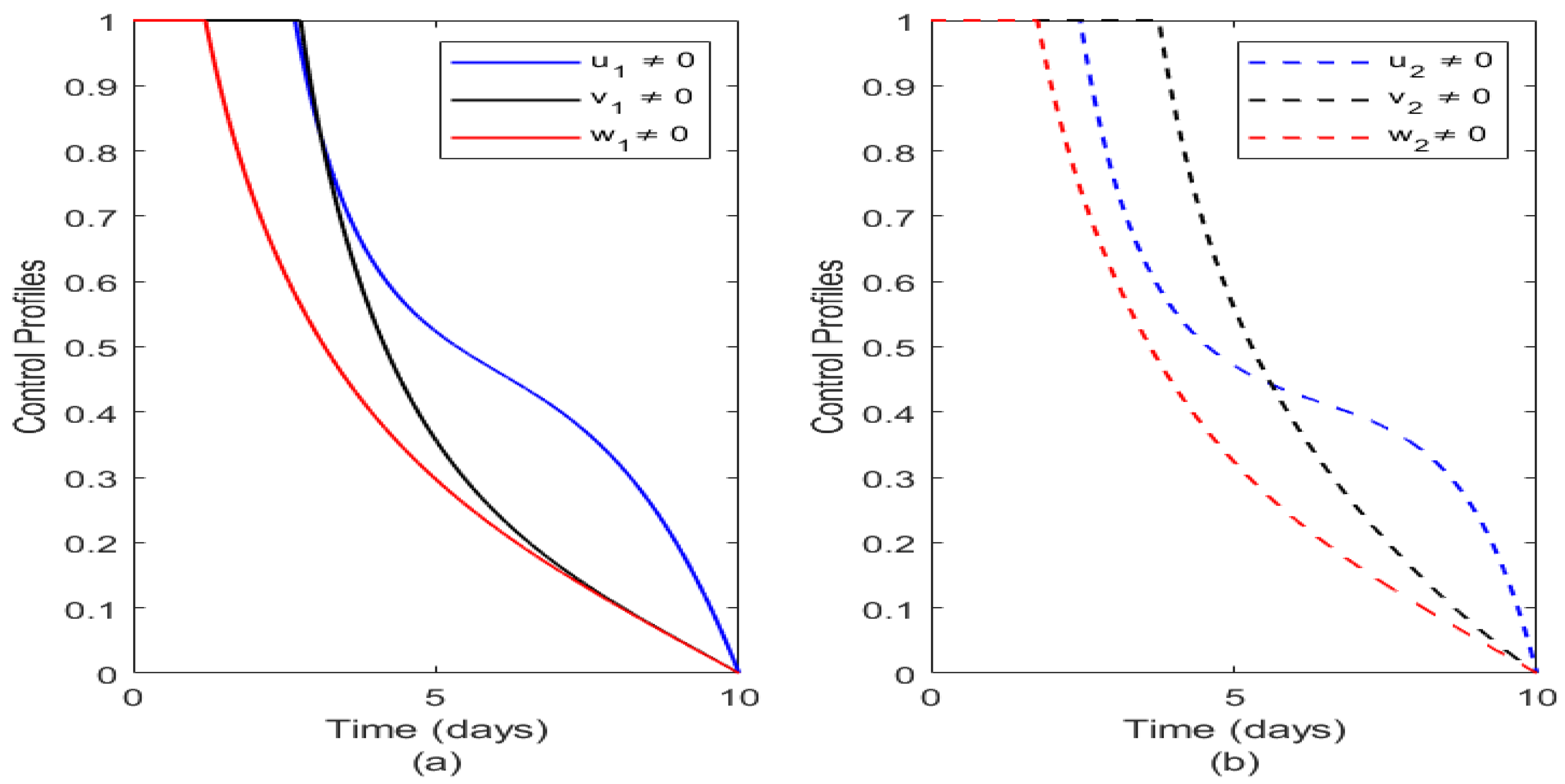
Here, we present the numerical solution of the optimal control problem. We start by considering the effect of the controls on different socio-economic status groups independently as seen in Figure 6 and then systematically show the effects of the optimal controls over the controls on the different classes as illustrated in Figure 7, Figure 8, Figure 9, Figure 10 and Figure 11. To illustrate this, we use the parameter values as given in Table 3 with the following assigned cost factors: $A_1=0.8$, $A_2=0.8$, $B_1=0.7$, $B_2=0.7$, $C_1=0.9$, $C_2=0.9$, $d_1=0.4$, $d_2=0.4$, $e_1=0.2$, $e_2=0.2$, $f_1=0.3$, $f_2=0.3$. We carried out iterative technique by employing the forward-backward algorithm postulated by Lenhart and Workman [38] to obtain the optimal control functions ($u_1,v_1,w_1$) and ($u_2,v_2,w_2)$ as shown in Figure 6. The figure shows that it is most appropriate or optimal to commence treatment early and to make it readily available to affected victims of typhoid fever and also to ensure that vaccination is adequately provided across all socio-economic communities and lastly adherence to good sanitation. This result is realistic, since it agrees with disease epidemiology in humans, and it supports good treatment and introduction of vaccination at an early stage before the onset of an epidemic while ensuring adequate treatment of individuals throughout the endemic period.

Figure 6 illustrates the optimal control profiles of the two socio-economic profiles. Here, vaccination is denoted by a thick red line on SEC 1 and a red dashed line on SEC 2. From Figure 6a, it is seen that the vaccination is very effective at the onset but diminishes with time on SEC 1. Also, we observe that for SEC 2, vaccination also thrives at the onset but diminishes over a period of time but when compared with vaccination on SEC 1; we show that vaccination in SEC 1 diminishes faster than that of SEC 2 and this could be attributed to the healthy or unhealthy activities carried out in either of the classes. Treatment on the other hand is denoted by the thick blue line on SEC 1 and the dashed blue line on SEC 2; it decreases almost at the same time in both socio-economics classes and this agrees with real-life intuition, as treatment may be helpful, but if the epidemic is not controlled, individuals requiring treatment may outnumber the available medical equipment and practitioners. This also shows that treatment when properly administered has same effect on both socio-economic classes. Finally, we have sanitation denoted by a thick black line in SEC 1 and a dashed black line in SEC 2. It is seen that sanitation plays a major role in reducing the impact of typhoid fever but it is more active on SEC 2 than SEC 1 and this readily agrees with the real-life scenario as high socio-economics class individuals tends to reside more in environments that are hygienic and they obey sanitation regulations.

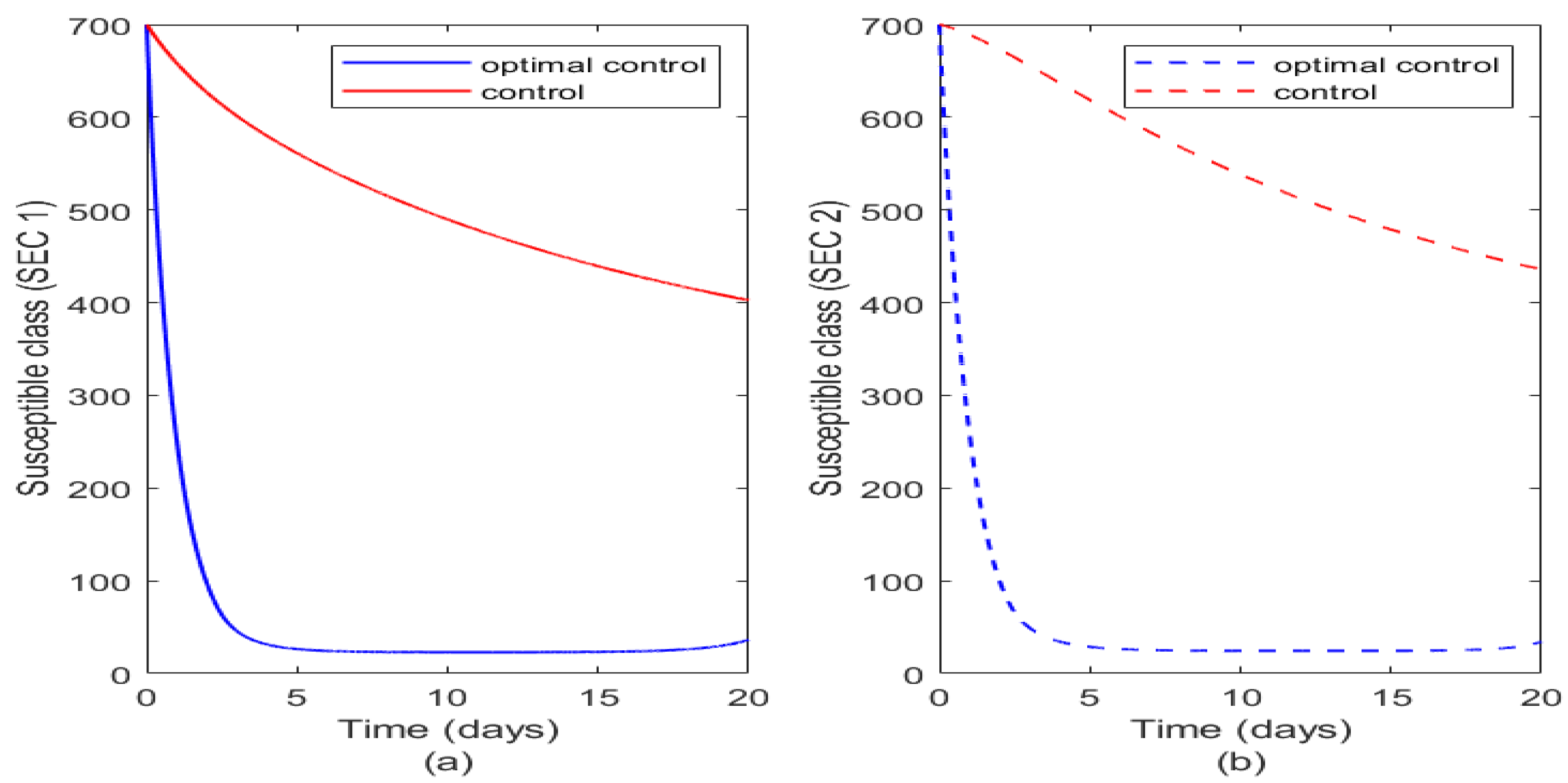
Figure 7 illustrates the impact of control and optimal control on susceptible humans in both socio-economic classes. The optimal control of vaccination completely reduces susceptibility to typhoid fever in both socio-economic class populations. Alternatively, just combining the controls has more impact on SEC 1 than on SEC 2 and this may be consequent of the fact that vaccination maybe more targeted to the SEC 1 population than the SEC 2 population.

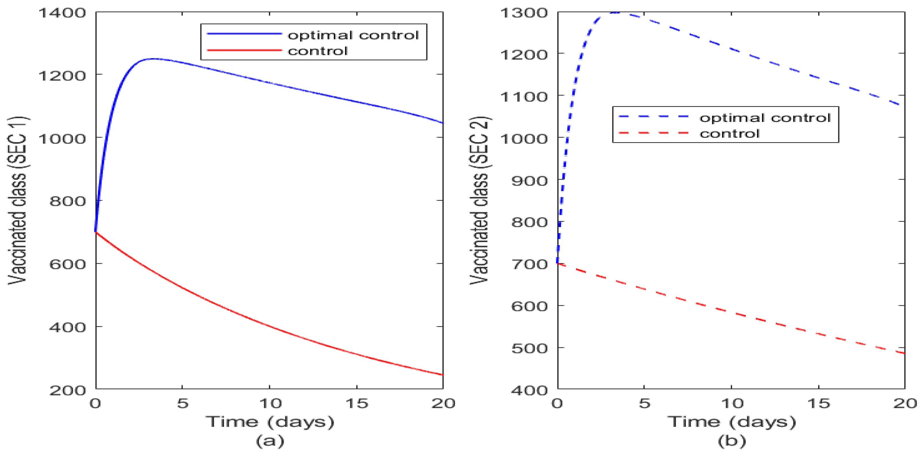
Figure 8 illustrates the effect of optimal control and controls on the vaccinated class. The vaccinated class in SEC 1 increases when vaccination is applied optimally but the impact of vaccination quickly reduces rather than in SEC 2 where there is more impact of optimal vaccination as shown in Figure 8b. Also, even without optimal control we can observe that the control by vaccination decreases more in SEC 1 when compared to SEC 2 even though we have more reduction in susceptibility in SEC 1 (Figure 8a). This agrees with our earlier prediction that vaccination diminishes faster in SEC 1 populations due to unhealthy practices and due to poor living standards with less immunity to diseases than those in SEC 2.

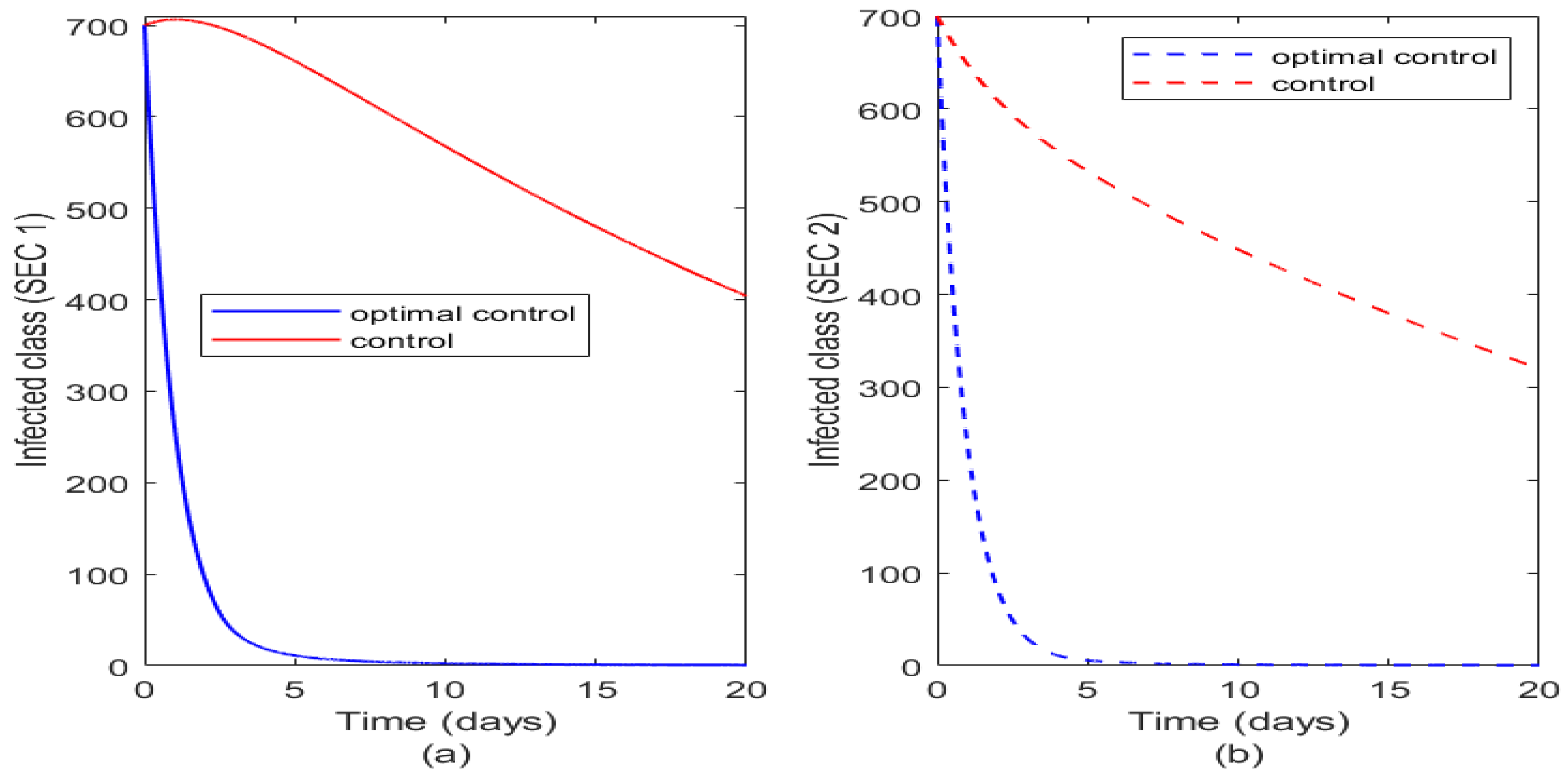
Figure 9 also illustrates the impact of optimal control and controls on the infected class of the two socio-economic classes. Optimal control has same effect on the two classes but the controls are more effective on SEC 2 than SEC 1. There is more reduction in the population of the infected class in SEC 2 (see Figure 9b) than in SEC 1 (Figure 9a) when the controls are not optimal. This agrees with real-life intuition as those in a higher socio-economic status tend to benefit more from disease-control strategies than those in a lower socio-economic status. But when either or all the controls are optimally used in both communities, it yields the same result.

From Figure 10 it is shown that with either controls or optimal control there is higher number of recovered humans in SEC 2 (Figure 10b) than in SEC 1 (Figure 10a) and this is attributed to good medical practices, good sanitation and early exposure to vaccination and generally good standards of living which boosts their immune system to enable them to recover faster even when infected.

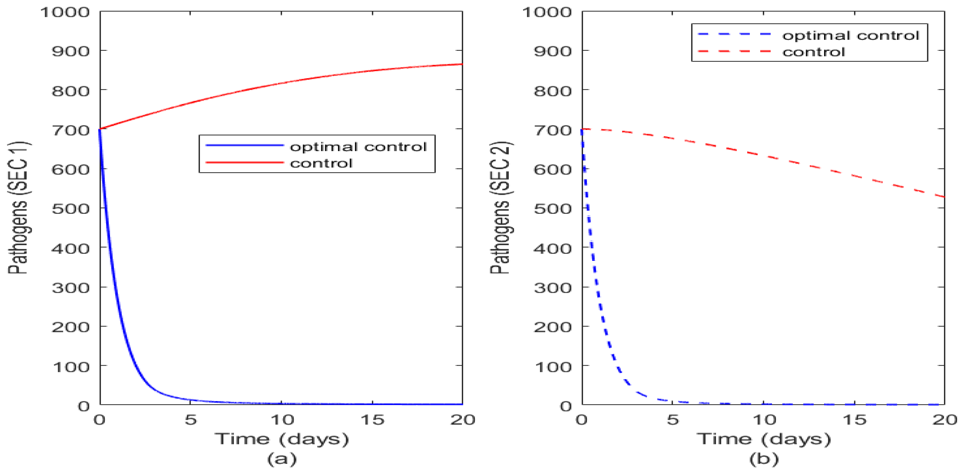
Finally, Figure 11 illustrates the impact of optimal control of sanitation on the pathogens in the two socio-economic classes. Analogous to other cases discussed, optimal sanitation reduces pathogens in both classes but just applying sanitation in relation to what is obtainable in the different socio-economic classes. It is seen that it is more effective in SEC 2 than in SEC 1.

7. Discussion

Typhoid fever is a fatal illness affecting humans, especially those in the lower socio-economic community with limited access to clean food and a neat environment. The disease can be prevented or controlled by adopting effective control intervention measures. Some of the effective control measures for decreasing typhoid fever infections in some affected communities include vaccination, treatment, and sanitation. Many countries/communities are comprised of individuals in different socio-economic classes. For more accurate results on the dynamics of typhoid fever, the socio-economic classes of individuals in the community must be taken into consideration. This study used a mathematical epidemiological model to analyze the influence of control interventions (vaccination, treatment, and sanitation) in decreasing typhoid fever in two socio-economic populations. By developing and analyzing a mathematical epidemiological model for typhoid fever for multiple socio-economic communities, the dynamics of the disease were explored. The results of our analysis showed that the disease can be eradicated from the two socio-economic classes using the control measures, provided that the basic reproduction number remained below 1. In contrast, when no control measure is introduced, the disease remains endemic in the community, especially in the lower socio-economic community. Further analysis revealed that under uniform movement rates, the lower SEC have a greater infected population, so control measures should be the focus on this class for faster disease eradication.

Next, the influence of each of the control measures was investigated numerically. Each of the control measures was found to have some influence in reducing typhoid fever. The combined effects of the multiple control measures yield better results when compared with the no-control measure and single control measure. Based on these findings, multiple control measures are highly recommended for controlling typhoid fever. However, if they are not available, any of the single control measures can be used because each of them is shown to have some positive influence in reducing infections in the two socio-economic communities.

Finally, we carried out optimal control analysis on our control model and it was observed that optimal control had an effect on both socio-economic classes, but optimizing treatment has more effect on SEC 2 than SEC 1 followed by vaccination and then sanitation. We also compared optimal control and controls on each of the classes in the two socio-economic classes. Our analysis showed that optimal control has a good effect on both classes even though it may diminish with time rather than using the controls collectively or independently. Overall, our analysis showed that more attention should be paid to communities of low socio-economic status in the event of typhoid fever epidemic. The result of this study agrees with the result formerly obtained by Mutua et. al. [29] but gives more insight on the required control measures and how these control measures helps in eradicating typhoid fever and most importantly shows which control is optimal when cost and availability might be an issue.

References

- World Health Organisation (WHO). August 2020. Available online: https://www.who.int/health-topics/typhoid#tab=tab$_1$ (accessed on 1 September 2023).
- Wain, J.; Hendriksen, R.S.; Mikoleit, M.L.; Keddy, K.H.; Ochiai, R.L. Typhoid fever. Lancet 2015, 385, 1136–1145. [Google Scholar] [CrossRef]
- Edward, S. A deterministic mathematical model for direct and indirect transmission dynamics of typhoid fever. Open Access Libr. J. 2017, 4, 1–16. [Google Scholar] [CrossRef]
- Moyer, C.A.; Johnson, C.; Kaselitz, E.; Aborigo, R. Using social autopsy to understand maternal, newborn, and child mortality in low-resource settings: A systematic review of the literature. Glob. Health Action 2017, 10, 1413917. [Google Scholar] [CrossRef]
- Snavely, M.E.; Maze, M.J.; Muiruri, C.; Ngowi, L.; Mboya, F.; Beamesderfer, J.; Rubach, M.P. Sociocultural and health system factors associated with mortality among febrile inpatients in Tanzania: A prospective social biopsy cohort study. Bmj Glob. Health 2018, 3, e000507. [Google Scholar] [CrossRef]
- Snavely, M.E.; Oshosen, M.; Msoka, E.F.; Karia, F.P.; Maze, M.J.; Blum, L.S.; Muiruri, C. If You Have No Money, You Might Die: A Qualitative Study of Sociocultural and Health System Barriers to Care for Decedent Febrile Inpatients in Northern Tanzania. Am. J. Trop. Med. Hyg. 2020, 103, 494. [Google Scholar] [CrossRef]
- Collins, O.C.; Robertson, S.L.; Govinder, K.S. Analysis of a waterborne disease model with socioeconomic classes. Math. Biosci. 2015, 269, 86–93. [Google Scholar] [CrossRef]
- Crump, J.A. Progress in typhoid fever epidemiology. Clin. Infect. Dis. 2019, 68 (Suppl. S1), S4–S9. [Google Scholar] [CrossRef]
- Crump, J.A.; Sjölund-Karlsson, M.; Gordon, M.A.; Parry, C.M. Epidemiology, clinical presentation, laboratory diagnosis, antimicrobial resistance, and antimicrobial management of invasive Salmonella infections. Clin. Microbiol. Rev. 2015, 28, 901–937. [Google Scholar] [CrossRef]
- Pitzer, V.E.; Feasey, N.A.; Msefula, C.; Mallewa, J.; Kennedy, N.; Dube, Q.; Heyderman, R.S. Mathematical modeling to assess the drivers of the recent emergence of typhoid fever in Blantyre, Malawi. Clin. Infect. Dis. 2015, 61 (Suppl. S4), S251–S258. [Google Scholar] [CrossRef]
- Bakach, I.; Just, M.R.; Gambhir, M.; Fung, I.C.H. Typhoid transmission: A historical perspective on mathematical model development. Trans. R. Soc. Trop. Med. Hyg. 2015, 109, 679–689. [Google Scholar] [CrossRef]
- Brauer, F. Mathematical epidemiology: Past, present, and future. Infect. Dis. Model. 2017, 2, 113–127. [Google Scholar]
- Kermack, W.O.; McKendrick, A.G. Contributions to the mathematical theory of epidemics. III—Further studies of the problem of endemicity. Proceedings of the Royal Society of London. Ser. Contain. Pap. Math. Phys. Character 1991, 141, 94–122. [Google Scholar]
- Kermack, W.O.; McKendrick, A.G. A contribution to the mathematical theory of epidemics. Proceedings of the royal society of london. Ser. Contain. Pap. Math. Phys. Character 1927, 115, 700–721. [Google Scholar]
- Cvjetanovic, B.B. Field trial of typhoid vaccines. Am. J. Public Health Nations Health 1957, 47, 578–581. [Google Scholar] [CrossRef]
- Matsebula, L.; Nyabadza, F.; Mushanyu, J. Mathematical analysis of typhoid fever transmission dynamics with seasonality and fear. Commun. Math. Biol. Neurosci. 2021. Available online: https://www.scik.org/index.php/cmbn/article/view/5590 (accessed on 12 September 2023).
- Irena, T.K.; Gakkhar, S. Modelling the dynamics of antimicrobial-resistant typhoid infection with environmental transmission. Appl. Math. Comput. 2021, 401, 126081. [Google Scholar]
- Collins, O.C.; Govinder, K.S. Stability analysis and optimal vaccination of a waterborne disease model with multiple water sources. Nat. Resour. Model 2016, 29, 426–447. [Google Scholar] [CrossRef]
- Onah, I.S.; Collins, O.C.; Madueme, P.G.U.; Mbah, G.C.E. Dynamical System Analysis and Optimal Control Measures of Lassa Fever Disease Model. Int. J. Math. Math. Sci. 2020, 2020, 7923125. [Google Scholar] [CrossRef]
- Van den Driessche, P.; Watmough, J. Reproduction numbers and sub-threshold endemic equilibria for compartmental models of disease transmission. Math. Biosci. 2002, 180, 29–48. [Google Scholar] [CrossRef]
- Tien, J.H.; Earn, D.J.D. Multiple Transmission Pathways and Disease Dynamics in a Waterborne Pathogen Model. Bull. Math. Biol. 2010, 72, 1506–1533. [Google Scholar]
- Castillo-Chavez, C.; Feng, Z.; Huang, W. On the Computation of R0 and Its Role on Global Stability. In Mathematical Approaches for Emerging and Reemerging Infectious Diseases. An Introduction, IMA; Springer: Berlin/Heidelberg, Germany, 2002; Volume 125. [Google Scholar]
- Robertson, S.L.; Eisenberg, M.C.; Tien, J.H. Heterogeneity in Multiple Transmission Pathways: Modelling the Spread of Cholera and Other Waterborne Disease in Networks with a Common Water Source. J. Biol. Dyn. 2013, 7, 254–275. [Google Scholar] [CrossRef] [PubMed]
- Onah, I.S.; Collins, O.C. Dynamical system analysis of a Lassa fever model with varying socioeconomic classes. J. Appl. Math. 2020, 2020, 2601706. [Google Scholar] [CrossRef]
- Collins, O.C.; Okeke, J.E. Analysis and control measures for Lassa fever model under socio-economic conditions. J. Physics: Conf. Ser. 2021, 1734, 012049. [Google Scholar] [CrossRef]
- Collins, O.C.; Okeke, J.E. Analysis and multiple control measures for a typhoid fever disease model. J. Physics: Conf. Ser. 2021, 1734, 012053. [Google Scholar] [CrossRef]
- King, A.A.; Lonides, E.L.; Pascual, M.; Bouma, M.J. Inapparent Infections and Cholera Dynamics. Nature 2008, 454, 877–881. [Google Scholar] [CrossRef]
- Mukandavire, Z.; Garira, W. HIV/AIDS model for assessing the effects of prophylactic sterilizing vaccines, condoms and treatment with amelioration. J. Biol. Syst. 2006, 14, 323–355. [Google Scholar] [CrossRef]
- Mutua, J.M.; Barker, C.T.; Vaidya, N.K. Modeling impacts of socioeconomic status and vaccination programs on typhoid fever epidemics. Electron. J. Differ. Equ. Conf. 2017, 24, 63–74. [Google Scholar]
- Lucas, M.E.S.; Deen, J.L.; Seidlein, L.; Wang, X.; Ampuero, J.; Puri, M.; Ali, M.; Ansaruzzaman, M.; Amos, J.; Macuamule, A.; et al. Effectiveness of Mass Oral Cholera Vaccination in Beira, Mozambique. N. Engl. J. Med. 2005, 352, 757–767. [Google Scholar] [CrossRef]
- Miller Neilan, R.L.; Schaefer, E.; Gaff, H.; Fister, K.R.; Lenhart, S. Modeling optimal intervention strategies for cholera. Bull. Math. Biol. 2010, 72, 2004–2018. [Google Scholar] [CrossRef]
- Kar, T.K.; Batabyal, A. Stability analysis and optimal control of an SIR epidemic model with vaccination. Biosystems 2011, 104, 127–135. [Google Scholar] [CrossRef]
- Agusto, F.B. Optimal chemoprophylaxis and treatment control strategies of a tuberculosis transmission model. World J. Model. Simul. 2009, 5, 163–173. [Google Scholar]
- Joshi, H.R. Optimal control of an HIV immunology model. Optim. Control. Appl. Methods 2002, 23, 199–213. [Google Scholar] [CrossRef]
- Onah, I.S.; Aniaku, S.E.; Ezugorie, O.M. Analysis and optimal control measures of diseases in cassava population. Optim. Control. Appl. Methods 2022, 43, 1450–1478. [Google Scholar] [CrossRef]
- Pontryagin, L.S. Mathematical Theory of Optimal Processes; CRC Press: Boca Raton, FL, USA, 1962. [Google Scholar]
- Mugabi, F.; Mugisha, J.; Nannyonga, B.; Kasumba, H.; Tusiime, M. Parameter-dependent transmission dynamics and optimal control of foot and mouth disease in a contaminated environment. J. Egypt. Math. Soc. 2019, 27, 53. [Google Scholar] [CrossRef]
- Lenhart, S.; Workman, J.T. Optimal Control Applied to Biological Models; CRC Press: New York, NY, USA, 2007. [Google Scholar]
Figure 1.
Plot illustrating the effects of vaccination rate on the dynamics of typhoid fever infections in SEC 1 and SEC 2.
Figure 2.
Plot illustrating the impact of vaccine efficacy on the dynamics of typhoid fever infections in SEC 1 and SEC 2.
Figure 3.
Plot illustrating the influence of treatment on the dynamics of typhoid fever infections in SEC 1 and SEC 2.
Figure 4.
Plot illustrating the influence of sanitation on the dynamics of typhoid fever infections in SEC 1 and SEC 2.
Figure 5.
Plot illustrating the impact of multiple control measures on the dynamics of typhoid fever infections in SEC 1 and SEC 2.
Figure 6.
Plot illustrating the control profiles of the two socio-economic classes. (a) illustrates the control profiles for SEC 1 while (b) illustrates control profiles for SEC 2.
Figure 7.
Plot illustrating effect of optimal control and controls on the two socio-economic classes. (a) illustrates the effect of optimal control and controls on susceptible class of SEC 1 while (b) illustrates the effect of optimal control and controls on susceptible class of SEC 2.
Figure 8.
Plot illustrating effect of optimal control and controls on the two socio-economic classes. (a) illustrates the effect of optimal control and controls on vaccinated class of SEC 1 while (b) illustrates the effect of optimal control and controls on vaccinated class of SEC 2.
Figure 9.
Plot illustrating effect of optimal control and controls on the two socio-economic classes. (a) illustrates the effect of optimal control and controls on infected class of SEC 1 while (b) illustrates the effect of optimal control and controls on infected class of SEC 2.
Figure 10.
Plot illustrating effect of optimal control and controls on the two socio-economic classes. (a) illustrates the effect of optimal control and controls on recovered class of SEC 1 while (b) illustrates the effect of optimal control and controls on recovered class of SEC 2.
Figure 11.
Plot illustrating effect of optimal control and controls on the two socio-economic classes. (a) illustrates the effect of optimal control and controls on pathogens in the environment of SEC 1 while (b) illustrates the effect of optimal control and controls on pathogens in the environment of SEC 2.