A Novel Nonlinear Dynamic Model Describing the Spread of Virus

Abstract

This study proposes a nonlinear mathematical model of virus transmission. The interaction between viruses and immune cells is investigated using phase-space analysis. Specifically, the work focuses on the dynamics and stability behavior of the mathematical model of a virus spread in a population and its interaction with human immune system cells. The endemic equilibrium points are found, and local stability analysis of all equilibria points of the related model is obtained. Further, the global stability analysis, either at disease-free equilibria or in endemic equilibria, is discussed by constructing the Lyapunov function, which shows the validity of the concern model. Finally, a simulated solution is achieved, and the relationship between viruses and immune cells is highlighted.

1. Introduction

Mathematical modeling of biological processes is a field of research that facilitates our understanding of complex biological systems and variables by simulating and analyzing several biological scenarios through specific models based on mathematical theories [1,2,3]. It provides a robust approach to describe mechanisms behind the dynamics occurring in biological processes by melting mathematical theories and models in the same pot with biological simulations [1]. This approach is playing a crucial role in predicting the spread rates of various major public health problems caused by viral diseases such as Ebola [4], influenza [5], cancer [6], Zika [7], Usutu [8], and COVID-19 [9].

Simultaneously, the field of mathematical modeling and simulations has gained considerable attention in various areas of human physiology, e.g., the analysis of muscle structure [10] and the study of brain activity [11,12]. Furthermore, mathematical modeling is also actively used to optimize medication usage and treatment processes [13,14,15]. In this study, we focused mainly on modeling and simulating the spread of viruses and the behavior of cells in the human immune system through the dynamical modeling approach. Dynamic models are widely recognized for their pivotal role in describing the interactions among uninfected cells, free viruses, and immune responses [16,17,18,19]. The latest study findings highlighted the ability of complex models to describe human biology. For instance, Nowak et al. proposed a three-dimensional dynamic model for viral infection, which utilized numerical methods from autonomous dynamical systems [17,18,19]. Giesl and Wendland characterized a Lyapunov function as a solution of a suitable linear first-order partial differential equation, approximating it using radial basis functions [20]. Yang and Wang formulated a mathematical model employing non-constant transmission rates, which varied with environmental conditions and the epidemiological status and reflected the impact of the ongoing disease control measures [21]. Despite significant efforts in designing mathematical models for virus dynamics, characterizing their behavior remains challenging. Even though several models have been proposed over the past two decades, their results bring different outcomes [22,23,24,25,26].

Kahajji et al. conducted a study focusing on the transmission dynamics of viruses, developing a separate mathematical model to describe the spread of the virus among animals in different regions. Their study highlights the importance of implementing effective campaigns to prevent individuals from moving between regions, promoting participation in quarantine centers, utilizing awareness campaigns targeted at virus prevention, and implementing security measures and health protocols within the region [27]. They estimated outbreak dynamics through mathematical modeling and provided decision guidelines for successful outbreak control. Furthermore, their model provided a valuable tool for estimating vaccination effectiveness and quantifying the impact of relaxing political measures, such as total lockdowns, shelter-in-place orders, and travel restrictions, for both low-risk subgroups and the population as a whole [28]. Moreover, Wang and Feng explored the combined effects of cell-free infection and cytokine-enhanced viral infection using a spatially heterogeneous PDE model considering cell reproduction, free-virus infection, and cytokine-enhanced viral infection [29]. Numerous studies have highlighted the importance of models and simulations in understanding complex biological phenomena and tackling emerging diseases. However, the diversity of biological factors affecting human health and the emergence of new diseases warrants further exploration.

Moreover, the mathematical approaches identified by the World Health Organization (WHO) can be essential in providing evidence-based information to healthcare decision-makers and policymakers [30].

In this study, we have theorized a nonlinear mathematical model of virus transmission. We consider the following mathematical model concerning the initial value problem for the following nonlinear systems:

$$\left\{\begin{array}{cc}\hfill \dot{T}\left(t\right)& =a-{\beta }_{1}V\left(t\right)T\left(t\right)-d_{1}T\left(t\right),\hfill \\ \hfill \dot{I}\left(t\right)& =qT\left(t\right)V\left(t\right)-{\beta }_{2}E\left(t\right)I\left(t\right)-d_{2}I\left(t\right),\hfill \\ \hfill \dot{E}\left(t\right)& ={\beta }_{3}I\left(t\right)E\left(t\right)-d_{3}E\left(t\right),\hfill \\ \hfill \dot{V}\left(t\right)& =bI\left(t\right)-cV\left(t\right)\hfill \end{array}\right.$$

(1)

$$T\left(t_0\right)=T_0,I\left(t_0\right)=I_0,E\left(t_0\right)=E_0,$$

(2)

$$V\left(t_0\right)=V_0,t_0\in \left[0,\right.\left.a\right),$$

where $T=T\left(t\right)$, $I=I\left(t\right)$, $E\left(t\right)$, and $V\left(t\right)$ denote the concentration of uninfected cells, infected cells, effector immune cells, and free viruses at time $t\in (0,a)$, respectively.

Uninfected cells are supplied at a rate a, and uninfected hepatocytes (target cells, T) are infected by virus V at decrease at rate ${\beta }_1$. The coefficients $d_i$ ($i=1,2,3$) take into account the natural death of $T\left(t\right)$, $I\left(t\right)$, and $E\left(t\right)$. The q coefficient is the rate constant characterizing infection. Therefore, q considers the number of uninfected cells coping with the virus, increasing infected cells’ quantity. In the literature, many authors considered ${\beta }_1$ equal to q [18]. However, in this study, we hypothesize that the rate of uninfected cells that are infected by the virus can be, in general, different from the rate of the decrease of the uninfected cells coping with the virus (i.e., ${\beta }_1\ne q$). It can be due to other mechanisms such as the administration of drugs or other processes [31].

Effector cells mediate infection by eliminating productively infected cells. At the beginning, effector immune cells E are supplied to the presence of a tumor, which is responsible for starting the immune response [32]. For the sake of clarity, the tumor dynamic is out of the scope of this study because of its complexity and debatable dynamics. Here, we considered tumors only as an example of an immune system onset system. In fact, during the early stages of tumor development, cytotoxic immune cells such as natural killer (NK) and CD8+ T cells recognize and eliminate the more immunogenic cancer cells. This first phase of elimination could select the proliferation of cancer cell variants that are less immunogenic and, therefore, invisible to immune detection. The variable $E\left(t\right)$ denotes the magnitude of the immune response, that is, the amount of virus-specific effector cells. Their rate of proliferation in response to an antigen is given by ${\beta }_{3}V\left(t\right)E\left(t\right)$. In the absence of stimulation, $E\left(t\right)$ decay at rate $d_3$. Infected cells are killed by $E\left(t\right)$ at rate ${\beta }_{2}E\left(t\right)I\left(t\right)$. These simple dynamics are derived from the kinetic interaction between effector immune and infected cells. The parameter ${\beta }_3$ denotes the immune system responsiveness, defined earlier as the growth rate of specific effector cells after encountering infected cells. The parameter ${\beta }_2$ specifies the rate at which effector cells kill infected cells. The infected cells produce new viruses at the rate of b. The constant $c>0$ is the rate at which the viruses are cleared [33,34,35].

2. Boundedness and Dissipativity

In this section, we showed that the model is bounded by negative divergence, positively invariant with respect to a region in ${\mathbb{R}}_{+}^4$, and dissipative. Since we aim to obtain biologically significant system solutions, the next results indicate that the positive octant is invariant and that the upper limits of the trajectories depend on the parameters.

We define

$$T\left(t\right)=x_1\left(t\right),I\left(t\right)=x_2\left(t\right),E\left(t\right)=x_3\left(t\right),V\left(t\right)=x_4\left(t\right).$$

Then, problems (1) and (2) are reduced to the following form:

$${\dot{x}}_1\left(t\right)=a-{\beta }_1{x}_4\left(t\right)x_1\left(t\right)-d_1{x}_1\left(t\right),$$

(3)

$${\dot{x}}_2\left(t\right)=q{x}_1\left(t\right)x_4\left(t\right)-{\beta }_2{x}_3\left(t\right)x_2\left(t\right)-d_2{x}_2\left(t\right),$$

$${\dot{x}}_3\left(t\right)={\beta }_3{x}_2\left(t\right)x_3\left(t\right)-d_3{x}_3\left(t\right),$$

$${\dot{x}}_4\left(t\right)=b{x}_2\left(t\right)-c{x}_4\left(t\right),$$

$$x_1\left(t_0\right)=x_{10},x_2\left(t_0\right)=x_{20},x_3\left(t_0\right)=x_{30},$$

(4)

$$x_4\left(t_0\right)=x_{40},t_0\in \left[0,\right.\left.a\right).$$

Let

$$x=x\left(t\right)=\left(x_1,x_2,x_3,x_4\right),x_j=x_j\left(t\right),j=1,2,3,4,$$

(5)

$$f_1\left(x\right)=a-{\beta }_1{x}_4\left(t\right)x_1\left(t\right)-d_1{x}_1\left(t\right)$$

$$f_2\left(x\right)=q{x}_1\left(t\right)x_4\left(t\right)-{\beta }_2{x}_3\left(t\right)x_2\left(t\right)-d_2{x}_2\left(t\right)$$

$$f_3\left(x\right)={\beta }_3{x}_2\left(t\right)x_3\left(t\right)-d_3{x}_3\left(t\right),f_4\left(x\right)=b{x}_2\left(t\right)-c{x}_4\left(t\right).$$

Here,

$${\mathbb{R}}_{+}^4=\left\{x=\left(x_1,x_2,x_3,x_4\right)\in {\mathbb{R}}^4,x_k>0\right\},$$

$$\mathsf{\Omega }=\left\{x\in {\mathbb{R}}_{+}^4:\right.{\beta }_3{x}_2-{\beta }_1{x}_4-{\beta }_2{x}_3\le d_1+d_2+d_3+c\}$$

Consider problems (3) and (4) with $t_0=0.$

Condition 1.

Assume the following assumption is satisfied

$${\beta }_1,{\beta }_2,d_1,d_2,d_3,c>0,{\beta }_3<0.$$

Theorem 1.

Let Condition 1 hold. Then, system $\left(3\right)$ has negative divergence and is dissipative in the domain $\mathsf{\Omega }\subset {\mathbb{R}}_{+}^4$.

Proof. 

Indeed, from $\left(3\right)$ and $\left(4\right)$, we have

$$\frac{\partial f_1}{\partial x_1}+\frac{\partial f_2}{\partial x_2}+\frac{\partial f_3}{\partial x_3}+\frac{\partial f_4}{\partial x_4}=-\left({\beta }_1{x}_4+d_1\right)-$$

$${\beta }_2{x}_3\left(t\right)-d_2+{\beta }_3{x}_2\left(t\right)-d_3-c.$$

Hence, by Condition 1, system $\left(3\right)$ is dissipative on the domain $\mathsf{\Omega }.$ However, there is no definition of Condition 1. □

3. The Local Stability of Equilibria Points

In this section, we derive the stability properties of equilibria points of system $\left(1\right)$. Let

$${\mathbb{R}}_{+}^4=\left\{x\in {\mathbb{R}}^4:x_i\ge 0,i=1,2,3,4\right\},B_r\left(\overline{x}\right)=\left\{x\in {\mathbb{R}}^4,{∥x-\overline{x}∥}_{{\mathbb{R}}^3}<r\right\}.$$

Condition 2.

Let

$$\frac{b{d}_3}{c}\ne d_1,b{d}_3\ne d_{1}c,\frac{b{a}_{33}{a}_{24}+a_{32}{a}_{23}c+a_{33}{a}_{21}{a}_{14}b}{a_{21}{a}_{14}b+b{a}_{33}{a}_{24}-a_{32}{a}_{23}}<0,d_3>{\beta }_3{\overline{x}}_2.$$

(6)

Theorem 2.

Assume that Condition 2 is satisfied. There is a point $P\left(x_1,x_2,x_3,x\right)$ that is an equilibrium point of system $\left(1\right)$ in ${\mathbb{R}}_{+}^4$.

Proof. 

It is sufficient to find the solution of the following system of algebraic equations in $x_1$, $x_2$, $x_3$, $x_4$:

$$a-\left({\beta }_1{x}_4-d_1\right)x_1=0,q{x}_1{x}_4-{\beta }_2{x}_3{x}_2-d_2{x}_2=0,$$

$${\beta }_3{x}_2{x}_3-d_3{x}_3=0,b{x}_2-c{x}_4=0.$$

(7)

From the first and second equations, we have

$${\overline{x}}_1=\frac{a}{\left({\beta }_1{x}_4-d_1\right)},q{x}_1{x}_4-{\beta }_2{x}_3{x}_2-d_2{x}_2=0.$$

(8)

From the third and fourth equations, we obtain

$$\left({\beta }_3{x}_2-d_3\right)x_3=0,x_4=\frac{b}{c}{x}_2.$$

(9)

If $x_3\ne 0$, we obtain that ${\overline{x}}_2=\frac{d_3}{{\beta }_3}$. By $\left(9\right)$, we deduced that ${\overline{x}}_4=\frac{b{d}_3}{c{\beta }_3}$. Hence, from $\left(8\right),$ we have

$${\overline{x}}_1=\frac{a}{\left(\frac{b{d}_3}{c}-d_1\right)},$$

$${\overline{x}}_3=\frac{1}{{\beta }_2{\overline{x}}_2}\left[q{\overline{x}}_1{\overline{x}}_4-d_2{\overline{x}}_2\right]=\frac{abq}{\left(b{d}_3-d_{1}c\right){\beta }_2}-\frac{d_2}{{\beta }_2}.$$

Thus, we obtain that system $\left(1\right)$ has a unique equalibrium point $P\left({\overline{x}}_1,{\overline{x}}_2,{\overline{x}}_3,{\overline{x}}_4\right)$, where

$${\overline{x}}_1=\frac{a}{\left(\frac{b{d}_3}{c}-d_1\right)},{\overline{x}}_2=\frac{d_3}{{\beta }_3},{\overline{x}}_3=\frac{abq}{\left(b{d}_3-d_{1}c\right){\beta }_2}-\frac{d_2}{{\beta }_2},{\overline{x}}_4=\frac{b{d}_3}{c{\beta }_3}.$$

(10)

□

Remark 1.

For the point to have the biological meaning of stability point $P\left({\overline{x}}_1,{\overline{x}}_2,{\overline{x}}_3,{\overline{x}}_4\right)$, it should be:

$$d_1<\frac{b{d}_3}{c},b{d}_3-d_{1}c>0,{\beta }_2{\overline{x}}_3+d_2>0.$$

(11)

We show here, the following results:

Theorem 3.

Assume that Condition 2 is satisfied. Suppose estimate $\left(11\right)$ holds. Then, the point $P\left({\overline{x}}_1,{\overline{x}}_2,{\overline{x}}_3,{\overline{x}}_4\right)$ is a locally stable point for the system of $\left(1\right).$

Proof. 

Consider the linearized matrix of $\left(1\right)$, i.e., the Jacobian matrıx according to system (1) at point $P\left({\overline{x}}_1,{\overline{x}}_2,{\overline{x}}_3,{\overline{x}}_4\right)$, which is the following:

$$A=\frac{Df}{Dx}=\left[\begin{array}{cccc}\frac{\partial f_1}{\partial x_1}& \frac{\partial f_1}{\partial x_2}& \frac{\partial f_1}{\partial x_3}& \frac{\partial f_1}{\partial x_4}\\ \frac{\partial f_2}{\partial x_1}& \frac{\partial f_2}{\partial x_2}& \frac{\partial f_2}{\partial x_3}& \frac{\partial f_2}{\partial x_4}\\ \frac{\partial f_3}{\partial x_1}& \frac{\partial f_3}{\partial x_2}& \frac{\partial f_3}{\partial x_3}& \frac{\partial f_3}{\partial x_4}\\ \frac{\partial f_4}{\partial x_1}& \frac{\partial f_4}{\partial x_2}& \frac{\partial f_4}{\partial x_2}& \frac{\partial f_4}{\partial x_3}\end{array}\right]=\left[\begin{array}{cccc}{a}_{11}& 0& 0& a_{14}\\ a_{21}& a_{22}& a_{23}& a_{24}\\ 0& a_{32}& a_{33}& 0\\ 0& b& 0& -c\end{array}\right],$$

(12)

where ${\beta }_3{x}_2\left(t\right)x_3\left(t\right)-d_3{x}_3\left(t\right)$

$$a_{11}=-\left({\beta }_1{\overline{x}}_4+d_1\right),a_{14}=-{\beta }_1{\overline{x}}_1,a_{21}=q{\overline{x}}_4,a_{22}=-\left({\beta }_2{\overline{x}}_3+d_2\right),$$

$$a_{23}=-{\beta }_2{\overline{x}}_2,a_{24}=q{\overline{x}}_1,a_{32}={\beta }_3{\overline{x}}_3,a_{32}={\beta }_3{\overline{x}}_3,a_{33}={\beta }_3{\overline{x}}_2-d_3.$$

(13)

The eigenvalues of matrix A can be found as the solutions of the following equations:

$$A-\lambda I=\left[\begin{array}{cccc}{a}_{11}-\lambda & 0& 0& a_{14}\\ a_{21}& a_{22}-\lambda & a_{23}& a_{24}\\ 0& a_{32}& a_{33}-\lambda & 0\\ 0& b& 0& -\left(c+\lambda \right)\end{array}\right]=$$

$$\left[a_{11}-\lambda \right]\left[\begin{array}{ccc}{a}_{22}-\lambda & a_{23}& a_{24}\\ a_{32}& a_{33}-\lambda & 0\\ b& 0& -\left(c+\lambda \right)\end{array}\right]-$$

$$a_{21}\left(i\right)\left[\begin{array}{ccc}0& 0& a_{14}\\ a_{32}& a_{33}-\lambda & 0\\ b& 0& -\left(c+\lambda \right)\end{array}\right]=$$

(14)

$$\left(a_{11}-\lambda \right)\left[\right.-\left(c+\lambda \right)\left(a_{22}-\lambda \right)\left(a_{33}-\lambda \right)-$$

$$b{a}_{24}\left(a_{33}-\lambda \right)+\left.a_{32}{a}_{23}\left(c+\lambda \right)\right]+a_{21}{a}_{14}b\left(a_{33}-\lambda \right)=0.$$

Let

$$\left(c+\lambda \right)\left(a_{22}-\lambda \right)\left(a_{33}-\lambda \right)=0,$$

i.e., ${\lambda }_1=-c$, ${\lambda }_2=a_{22}$, and ${\lambda }_3=a_{33}$ are the eigenvalues of A. Then, other solutions of A can be obtained by solving the equation

$$b{a}_{24}\left(a_{33}-\lambda \right)+\left.a_{32}{a}_{23}\left(c+\lambda \right)\right]+a_{21}{a}_{14}b\left(a_{33}-\lambda \right)=$$

(15)

$$\left(a_{21}{a}_{14}b+b{a}_{33}{a}_{24}-a_{32}{a}_{23}\right)\lambda =b{a}_{33}{a}_{24}+a_{32}{a}_{23}c+a_{33}{a}_{21}{a}_{14}b=0$$

By solving Equation $\left(15\right)$, we obtain the fourth eigenvalue of matrix A

$${\lambda }_4=\frac{b{a}_{33}{a}_{24}+a_{32}{a}_{23}c+a_{33}{a}_{21}{a}_{14}b}{a_{21}{a}_{14}b+b{a}_{33}{a}_{24}-a_{32}{a}_{23}}.$$

For local stability of system $\left(1\right),$ it is sufficient to show that all eigenvalues of matrix A are negative. Indeed, by $\left(10\right)$ and $\left(11\right)$, we have

$${\lambda }_1=-c<0,{\lambda }_2=a_{22}=-\left({\beta }_2{\overline{x}}_3+d_2\right)<0,$$

(16)

$${\lambda }_3=a_{33}={\beta }_3{\overline{x}}_2-d_3<0,{\lambda }_4=\frac{b{a}_{33}{a}_{24}+a_{32}{a}_{23}c+a_{33}{a}_{21}{a}_{14}b}{a_{21}{a}_{14}b+b{a}_{33}{a}_{24}-a_{32}{a}_{23}}<0.$$

By assumption $\left(11\right)$, and by $\left(10\right)$, we see that,

$${\overline{x}}_1\ge 0,{\overline{x}}_2\ge 0,{\overline{x}}_3\ge 0,{\overline{x}}_4\ge 0.$$

Hence, by $\left(16\right)$, we obtain

$${\lambda }_1<0,{\lambda }_2<0,{\lambda }_3<0.$$

Moreover, it should be

$${\lambda }_4=\frac{b{\beta }_{3}q{\overline{x}}_1{\overline{x}}_2-c{\beta }_2{\beta }_3{\overline{x}}_2{\overline{x}}_3-b{\beta }_1{\beta }_{3}q{\overline{x}}_1{\overline{x}}_2{x}_4}{-b{\beta }_{1}q{\overline{x}}_1{\overline{x}}_4+b{\beta }_{3}q{\overline{x}}_1{\overline{x}}_2+{\beta }_2{\beta }_3{\overline{x}}_2{\overline{x}}_3}<0.$$

(17)

Estimate $\left(17\right)$ is satisfied if:

$$b{\beta }_{3}q{\overline{x}}_1{\overline{x}}_2-c{\beta }_2{\beta }_3{\overline{x}}_2{\overline{x}}_3-b{\beta }_1{\beta }_{3}q{\overline{x}}_1{\overline{x}}_2{\overline{x}}_4<0,$$

(18)

$$-b{\beta }_{1}q{\overline{x}}_1{\overline{x}}_4+b{\beta }_{3}q{\overline{x}}_1{\overline{x}}_2+{\beta }_2{\beta }_3{\overline{x}}_2{\overline{x}}_3>0.$$

or

$$b{\beta }_{3}q{\overline{x}}_1{\overline{x}}_2-c{\beta }_2{\beta }_3{\overline{x}}_2{\overline{x}}_3-b{\beta }_1{\beta }_{3}q{\overline{x}}_1{\overline{x}}_2{\overline{x}}_4>0,$$

(19)

$$-b{\beta }_{1}q{\overline{x}}_1{\overline{x}}_4+b{\beta }_{3}q{\overline{x}}_1{\overline{x}}_2+{\beta }_2{\beta }_3{\overline{x}}_2{x}_3<0.$$

Since $x_k\ge 0$, the second inequality in $\left(18\right)$ is satisfied for all $x\in {\mathbb{R}}_{+}^4$ when

$$b{\beta }_{3}q{\overline{x}}_1{\overline{x}}_2-c{\beta }_2{\beta }_3{\overline{x}}_2{\overline{x}}_3-b{\beta }_1{\beta }_{3}q{\overline{x}}_1{\overline{x}}_2{\overline{x}}_4<0,$$

i.e., by $\left(10\right)$, if

$$\frac{bqa{d}_{3}c}{b{d}_3-d_{1}c}<\frac{c{d}_{3}abq+b{\beta }_{1}qa{d}_3^{2}b}{\left(b{d}_3-d_{1}c\right)}.$$

By assumption $\left(11\right)$, the above inequality is satisfied when

$$d_{3}c<c{d}_3+{\beta }_1{d}_3^{2}b,$$

and it is clear that it holds for all $x\in {\mathbb{R}}_{+}^4$. Since $b{\beta }_{1}q{\overline{x}}_1{\overline{x}}_4+b{\beta }_{3}q{\overline{x}}_1{\overline{x}}_2+{\beta }_2{\beta }_3{\overline{x}}_2{\overline{x}}_3\ge 0$ for all $x\in {\mathbb{R}}_{+}^4$, inequality $\left(19\right)$ is not satisfied in ${\mathbb{R}}_{+}^4$. Hence, we obtained that all eigenvalues of the matrix are negative under our assumptions. □

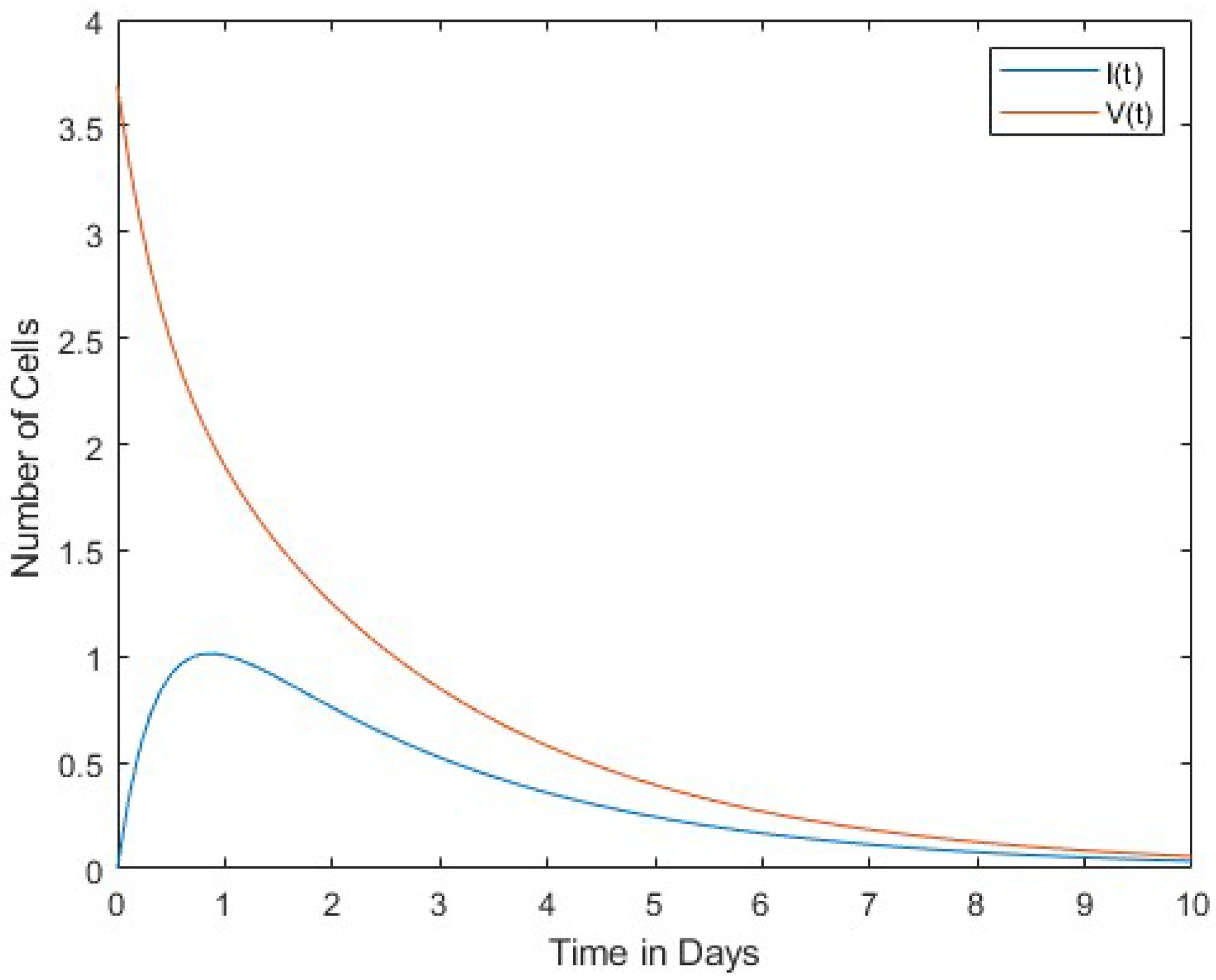
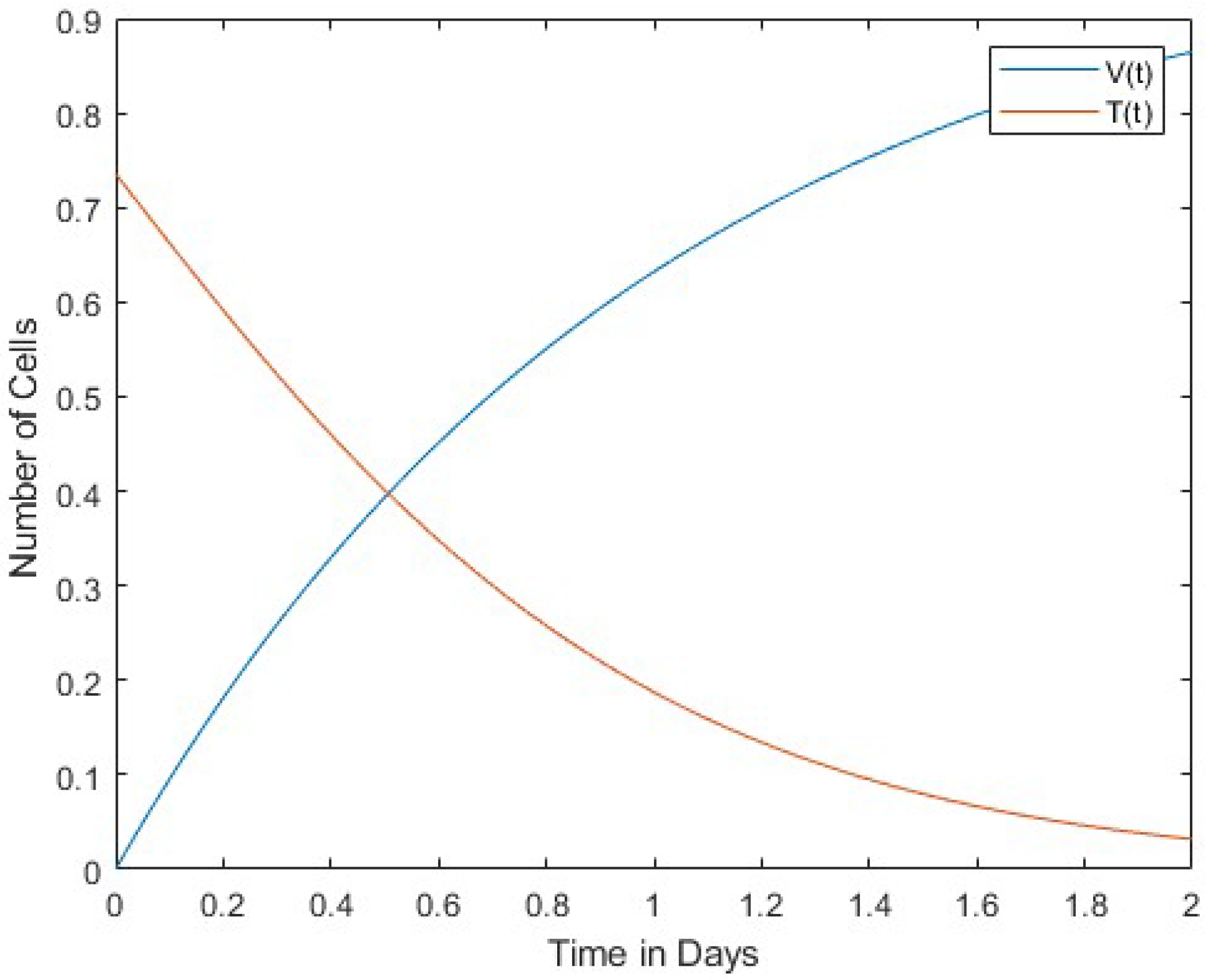
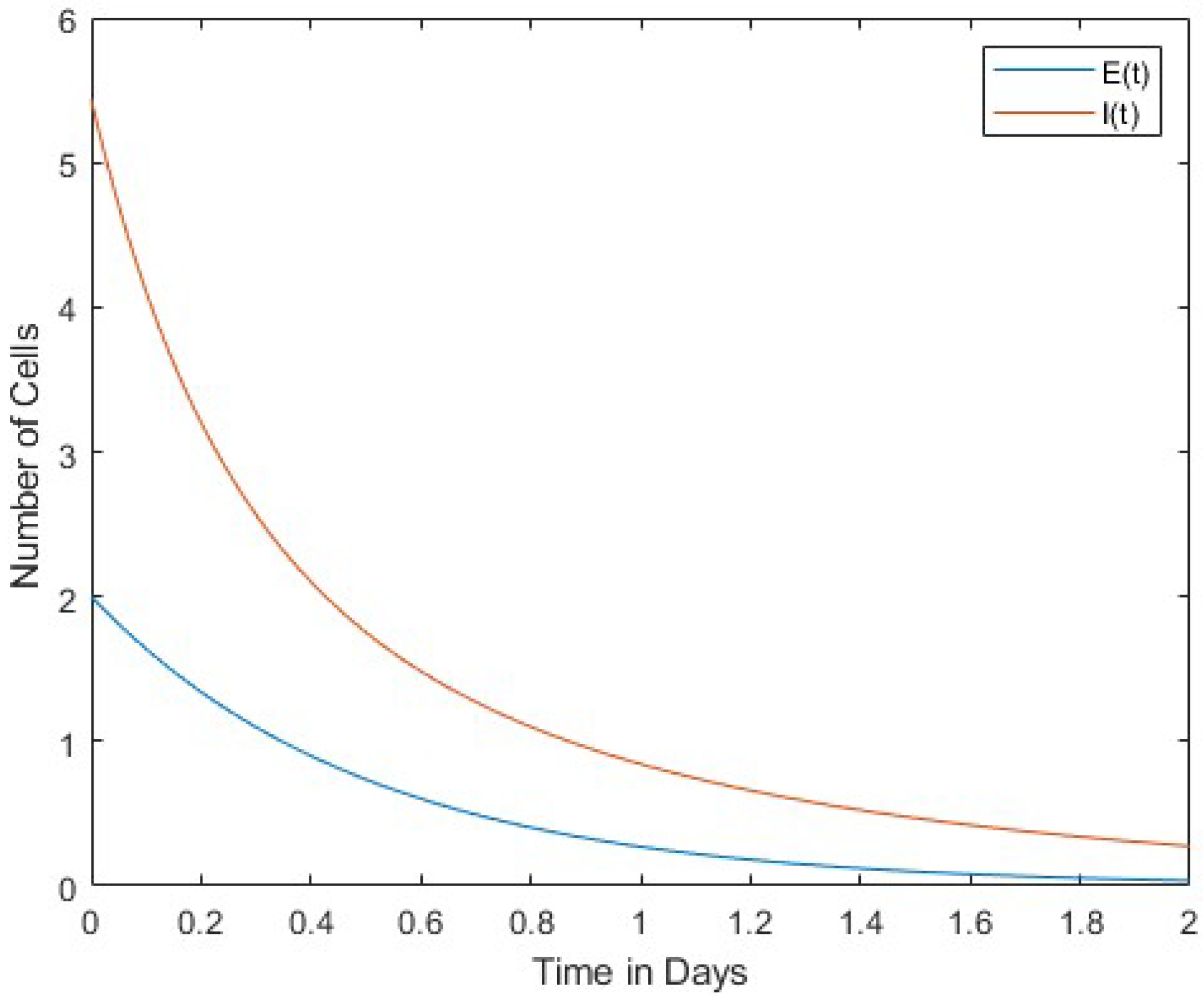
In Figure 1, we compare the number of viruses with the number of infected cells. Both the number of viruses and the number of infected cells decrease over time. Figure 2 compares the number of viruses with the number of uninfected cells. In this case, the rates of change between the two are in inverse proportion to each other. Finally, Figure 3 shows a comparison between the number of infected cells and the number of effector immune cells. It is noticeable that both the infected cells and the immune cells in this figure rapidly decrease over time.

4. Lyapunov Stability of Equilibria Points

Let $E\left(\overline{x}\right)$ be an equilibrium point, where $\overline{x}=\left({\overline{x}}_1,{\overline{x}}_2,{\overline{x}}_3,{\overline{x}}_4\right)\in {\mathbb{R}}_{+}^4$ is defined by $\left(10\right)$. In this section, we show the following results: let $A=A\left(\overline{x}\right)$ be the linearized matrix with respect to the equilibrium $E\left(\overline{x}\right)$ point defined by $\left(12\right)$, i.e.,

$$A=\left[\begin{array}{cccc}{a}_{11}& 0& 0& a_{14}\\ a_{21}& a_{22}& a_{23}& a_{24}\\ 0& a_{32}& a_{33}& 0\\ 0& b& 0& -c\end{array}\right],$$

where $a_{ij}$ are defined by $\left(13\right)$. We consider the Lyapunov equation

$$BA+A^{T}B=-I,B=B\left(\overline{x}\right)=\left[\begin{array}{cccc}{b}_{11}& b_{12}& b_{13}& b_{14}\\ b_{21}& b_{22}& b_{23}& b_{24}\\ b_{31}& b_{32}& b_{33}& b_{34}\\ b_{41}& b_{42}& b_{43}& b_{44}\end{array}\right],b_{ij}=b_{ji}.$$

(20)

It is clear that

$$BA=\left[\begin{array}{cccc}{b}_{11}& b_{12}& b_{13}& b_{14}\\ b_{21}& b_{22}& b_{23}& b_{24}\\ b_{31}& b_{32}& b_{33}& b_{34}\\ b_{41}& b_{42}& b_{43}& b_{44}\end{array}\right]\left[\begin{array}{cccc}{a}_{11}& 0& 0& a_{14}\\ a_{21}& a_{22}& a_{23}& a_{24}\\ 0& a_{32}& a_{33}& 0\\ 0& b& 0& -c\end{array}\right]=$$

$$\left[\begin{array}{cccc}-a_{11}{b}_{11}+a_{21}{b}_{12}& a_{22}{b}_{12}+a_{32}{b}_{13}+b{b}_{14}& a_{23}{b}_{12}+a_{33}{b}_{13}& a_{14}{b}_{11}+a_{24}{b}_{12}-c{b}_{14}\\ a_{11}{b}_{21}+a_{21}{b}_{22}-& a_{22}{b}_{22}+a_{32}{b}_{23}+b{b}_{24}& a_{23}{b}_{22}+a_{33}{b}_{23}& a_{14}{b}_{21}+a_{24}{b}_{22}-c{b}_{24}\\ a_{11}{b}_{31}+a_{21}{b}_{32}-& a_{22}{b}_{32}+a_{32}{b}_{33}+b{b}_{34}& a_{23}{b}_{32}+a_{33}{b}_{33}& a_{14}{b}_{31}+a_{24}{b}_{32}-c{b}_{34}\\ a_{11}{b}_{41}+a_{21}{b}_{42}-& a_{22}{b}_{42}+a_{32}{b}_{43}+b{b}_{44}& a_{23}{b}_{42}+a_{33}{b}_{43}& a_{14}{b}_{41}+a_{24}{b}_{42}-c{b}_{44}\end{array}\right],$$

$$A^{T}B=\left[\begin{array}{cccc}-a_{11}& a_{21}& 0& 0\\ 0& a_{22}& a_{32}& b\\ 0& a_{23}& -a_{33}& 0\\ a_{14}& a_{24}& 0& -c\end{array}\right]\left[\begin{array}{cccc}{b}_{11}& b_{12}& b_{13}& b_{14}\\ b_{21}& b_{22}& b_{23}& b_{24}\\ b_{31}& b_{32}& b_{33}& b_{34}\\ b_{41}& b_{42}& b_{43}& b_{44}\end{array}\right]=$$

$$\left[\begin{array}{cccc}{a}_{11}{b}_{11}+a_{21}{b}_{21}& a_{11}{b}_{12}+a_{21}{b}_{22}& a_{11}{b}_{13}+a_{21}{b}_{23}& a_{11}{b}_{14}+a_{21}{b}_{24}\\ a_{22}{b}_{21}+a_{32}{b}_{31}+b{b}_{41}& a_{22}{b}_{22}+a_{32}{b}_{32}+b{b}_{42}& a_{22}{b}_{23}+a_{32}{b}_{33}+b{b}_{43}& a_{22}{b}_{24}+a_{32}{b}_{34}+b{b}_{44}\\ a_{23}{b}_{21}+a_{33}{b}_{31}& a_{23}{b}_{22}+a_{33}{b}_{32}& a_{23}{b}_{23}+a_{33}{b}_{33}& a_{23}{b}_{24}+a_{33}{b}_{34}\\ -a_{14}{b}_{11}+a_{24}{b}_{21}-c{b}_{41}& a_{14}{b}_{12}+a_{24}{b}_{22}-c{b}_{42}& a_{14}{b}_{13}+a_{24}{b}_{23}-c{b}_{43}& a_{14}{b}_{14}+a_{24}{b}_{24}-c{b}_{44}\end{array}\right].$$

$\left(20\right)$ reduced to the following equation

$$BA+A^{T}B=\left[\begin{array}{cccc}{g}_{11}& g_{12}& g_{13}& g_{14}\\ g_{21}& g_{22}& g_{23}& g_{24}\\ g_{31}& g_{32}& g_{33}& g_{34}\\ g_{41}& g_{42}& g_{43}& g_{44}\end{array}\right]=-I,$$

(21)

where

$$g_{11}=2a_{11}{b}_{11}+2a_{21}{b}_{12}=-1,$$

$$g_{12}=\left(a_{11}+a_{22}\right)b_{12}+a_{32}{b}_{13}+b{b}_{14}+a_{21}{b}_{22}=0,$$

$$g_{13}=a_{23}{b}_{12}+\left(a_{11}+a_{33}\right)b_{13}+a_{21}{b}_{23}=0,$$

$$g_{14}=a_{14}{b}_{11}+a_{24}{b}_{12}+\left(a_{11}-c\right)b_{14}+a_{21}{b}_{24}=0,$$

$$g_{22}=2a_{22}{b}_{22}+2a_{32}{b}_{23}+2b{b}_{24}=-1,$$

$$g_{23}=a_{23}{b}_{22}+\left(a_{22}+a_{33}\right)b_{23}+a_{32}{b}_{33}+b{b}_{34}=0,$$

(22)

$$g_{24}=a_{14}{b}_{12}+a_{24}{b}_{22}+\left(a_{22}-c\right)b_{24}+a_{23}{b}_{34}+b{b}_{44}=0,$$

$$g_{33}=2a_{23}{b}_{23}+2a_{33}{b}_{33}=-1,$$

$$g_{34}=a_{14}{b}_{13}+a_{24}{b}_{23}+\left(a_{33}-c\right)b_{34}+a_{23}{b}_{24}=0,$$

$$g_{44}=2a_{14}{b}_{14}+2a_{24}{b}_{24}-2c{b}_{44}=-1.$$

Main and associated determinants of system $\left(22\right)$ in $b_{11},b_{12},$ $b_{13},b_{14},b_{22},b_{23},b_{24},b_{33},b_{34},$ $b_{44}$ are the following

$$\Delta =\left|\begin{array}{cccccccccc}2a_{11}& 2a_{21}& 0& 0& 0& 0& 0& 0& 0& 0\\ 0& a_{11}+a_{22}& a_{11}+a_{33}& a_{21}& 0& 0& 0& 0& 0& 0\\ 0& a_{23}& a_{11}+a_{33}& 0& 0& a_{21}& 0& 0& 0& 0\\ a_{14}& a_{24}& 0& \left(a_{11}-c\right)& 0& 0& a_{21}& 0& 0& 0\\ 0& 0& 0& 0& 2a_{22}& 2a_{32}& 2b& 0& 0& 0\\ 0& 0& 0& 0& a_{23}& a_{22}+a_{33}& 0& a_{32}& b& 0\\ 0& a_{14}& 0& 0& a_{24}& 0& \left(a_{22}-c\right)& 0& a_{23}& b\\ 0& 0& 0& 0& 0& 2a_{23}& 0& 2a_{33}& 0& 0\\ 0& 0& a_{14}& 0& 0& a_{24}& a_{23}& 0& \left(a_{33}-c\right)& 0\\ 0& 0& 0& 2a_{14}& 0& 0& 2a_{24}& 0& 0& -2cb\end{array}\right|,$$

$${\Delta }_1=\left|\begin{array}{cccccccccc}-1& 2a_{21}& 0& 0& 0& 0& 0& 0& 0& 0\\ 0& a_{11}+a_{22}& a_{11}+a_{33}& a_{21}& 0& 0& 0& 0& 0& 0\\ 0& a_{23}& a_{11}+a_{33}& 0& 0& a_{21}& 0& 0& 0& 0\\ -0& a_{24}& 0& \left(a_{11}-c\right)& 0& 0& a_{21}& 0& 0& 0\\ -1& 0& 0& 0& 2a_{22}& 2a_{32}& 2b& 0& 0& 0\\ 0& 0& 0& 0& a_{23}& a_{22}+a_{33}& 0& a_{32}& b& 0\\ 0& a_{14}& 0& 0& a_{24}& 0& \left(a_{22}-c\right)& 0& a_{23}& b\\ -1& 0& 0& 0& 0& 2a_{23}& 0& 2a_{33}& 0& 0\\ 0& 0& a_{14}& 0& 0& a_{24}& a_{23}& 0& \left(a_{33}-c\right)& 0\\ -1& 0& 0& 2a_{14}& 0& 0& 2a_{24}& 0& 0& -2cb\end{array}\right|,$$

$${\Delta }_2=\left|\begin{array}{cccccccccc}2a_{11}& -1& 0& 0& 0& 0& 0& 0& 0& 0\\ 0& 0& a_{11}+a_{33}& a_{21}& 0& 0& 0& 0& 0& 0\\ 0& 0& a_{11}+a_{33}& 0& 0& a_{21}& 0& 0& 0& 0\\ a_{14}& 0& 0& \left(a_{11}-c\right)& 0& 0& a_{21}& 0& 0& 0\\ 0& -1& 0& 0& 2a_{22}& 2a_{32}& 2b& 0& 0& 0\\ 0& 0& 0& 0& a_{23}& a_{22}+a_{33}& 0& a_{32}& b& 0\\ 0& 0& 0& 0& a_{24}& 0& \left(a_{22}-c\right)& 0& a_{23}& b\\ 0& -1& 0& 0& 0& 2a_{23}& 0& 2a_{33}& 0& 0\\ 0& 0& a_{14}& 0& 0& a_{24}& a_{23}& 0& \left(a_{33}-c\right)& 0\\ 0& -1& 0& 2a_{14}& 0& 0& 2a_{24}& 0& 0& -2cb\end{array}\right|,$$

$$\dots$$

$${\Delta }_{10}=\left|\begin{array}{cccccccccc}2a_{11}& 2a_{21}& 0& 0& 0& 0& 0& 0& 0& -1\\ 0& a_{11}+a_{22}& a_{11}+a_{33}& a_{21}& 0& 0& 0& 0& 0& 0\\ 0& a_{23}& a_{11}+a_{33}& 0& 0& a_{21}& 0& 0& 0& 0\\ a_{14}& a_{24}& 0& \left(a_{11}-c\right)& 0& 0& a_{21}& 0& 0& 0\\ 0& 0& 0& 0& 2a_{22}& 2a_{32}& 2b& 0& 0& -1\\ 0& 0& 0& 0& a_{23}& a_{22}+a_{33}& 0& a_{32}& b& 0\\ 0& a_{14}& 0& 0& a_{24}& 0& \left(a_{22}-c\right)& 0& a_{23}& 0\\ 0& 0& 0& 0& 0& 2a_{23}& 0& 2a_{33}& 0& -1\\ 0& 0& a_{14}& 0& 0& a_{24}& a_{23}& 0& \left(a_{33}-c\right)& 0\\ 0& 0& 0& 2a_{14}& 0& 0& 2a_{24}& 0& 0& -1\end{array}\right|.$$

We assume that $\Delta \ne 0$. Then, by solving $\left(22\right)$ with respect to $b_{ıj}$ by the Kramer method, we obtain

$$b_{11}=\frac{{\Delta }_1}{\Delta },b_{12}=b_{21}=\frac{{\Delta }_2}{\Delta },...,b_{44}=\frac{{\Delta }_n}{\Delta }.$$

(23)

Theorem 4.

Assume Condition 2 holds, $\Delta \ne 0$. Suppose $a_{ij}$ such that $b_{ii}>0$, $i=1,2,3,4$, $b_{ij}\ge 0$ for $i,j=1,2,3,4$, when $i\ne j$. Then, system $\left(3\right)$ is asymptotically stable at the equilibrium point $E\left(\overline{x}\right)$ in the sense of Lyapunov.

Proof. 

By assumptions, the function $P_A\left(x\right)$ is associated with matrix A, defined by

$$P_B\left(x\right)=x^{T}Bx=\sum _{i,j=1}^4{b}_{ij}{x}_i{x}_j,$$

which is positively defined in ${\mathbb{R}}^4.$ Hence, all eigenvalues ${\lambda }_1,{\lambda }_2,{\lambda }_3,{\lambda }_4$ of the matrix $B=B\left(\overline{x}\right)$ are positive in ${\mathbb{R}}^4$, i.e., $P_B\left(x\right)$ is a positive defined Lyapunov function candidate (see, e.g., [22,23]) by Corollary 8.2 [12]. We need now to determine a domain $\mathsf{\Omega }$ on which ${\dot{P}}_B\left(x\right)$ is negatively defined. By assuming $x_k\ge 0$, $k=1,2,3,4$, we will find the solution set of the following inequality

$$f_1\left(x\right)=a-{\beta }_1{x}_4\left(t\right)x_1\left(t\right)-d_1{x}_1\left(t\right)$$

$$f_2\left(x\right)=q{x}_1\left(t\right)x_4\left(t\right)-{\beta }_2{x}_3\left(t\right)x_2\left(t\right)-d_2{x}_2\left(t\right)$$

$$f_3\left(x\right)={\beta }_3{x}_2\left(t\right)x_3\left(t\right)-d_3{x}_3\left(t\right),f_4\left(x\right)=b{x}_2\left(t\right)-c{x}_4\left(t\right).$$

$${\dot{P}}_B\left(x\right)=\sum _{j=1}^4\frac{\partial {\dot{P}}_B}{\partial x_j}{f}_j\left(x\right)=$$

$$2\left(b_{11}{x}_1+b_{12}{x}_2+b_{13}{x}_3+b_{14}{x}_4\right)\left(a-{\beta }_1{x}_4{x}_1-d_1{x}_1\right)+$$

$$2\left(b_{21}{x}_1+b_{22}{x}_2+b_{23}{x}_3+b_{24}{x}_4\right)\left(q{x}_1{x}_4-{\beta }_2{x}_3{x}_2-d_2{x}_2\right)+$$

$$2\left(b_{31}{x}_1+b_{32}{x}_2+b_{33}{x}_3+b_{34}{x}_4\right)\left({\beta }_3{x}_2{x}_3-d_3{x}_3\right)+$$

(24)

$$2\left(b_{31}{x}_1+b_{32}{x}_2+b_{33}{x}_3+b_{34}{x}_4\right)\left(b{x}_2-c{x}_4\right)\le 0.$$

Hence, system $\left(3\right)$ is asymptotically stable at $E\left(\overline{x}\right)$ in the Lyapunov sense when

$$a-{\beta }_1{x}_4{x}_1-d_1{x}_1\le 0,q{x}_1{x}_4-{\beta }_2{x}_3{x}_2-d_2{x}_2\le 0,$$

$${\beta }_3{x}_2{x}_3-d_3{x}_3\le 0,b{x}_2-c{x}_4,$$

i.e., system $\left(3\right)$ is asymptotically stable at $E\left(\overline{x}\right)$ in the Lyapunov sense in the following domain:

$${\mathsf{\Omega }}_1=\{x\in {\mathbb{R}}_{+}^4:\left({\beta }_1{x}_4+d_1\right)x_1\ge a,\left({\beta }_2{x}_3+d_2\right)x_2\ge q{x}_1{x}_4,$$

$${\beta }_3{x}_2\le d_3,x_4\ge \frac{b}{c}{x}_2\}.$$

(25)

□

Theorem 5.

Assume Condition 2 holds, $\Delta \ne 0$. Suppose $a_{ij}$ such that $b_{ii}>0$, $i=1,2,3,4$ and $b_{ij}\le 0$ for $i,j=1,2,3,4$ when $i\ne j$. Then, system $\left(3\right)$ is asymptotically stable at the equilibrium point $E\left(\overline{x}\right)$ in the sense of Lyapunov.

Proof. 

$$P_B\left(x\right)=x^{T}Bx=\sum _{i,j=1}^4{b}_{ij}{x}_i{x}_j=$$

$$\frac{1}{4}{b}_{11}{\left(x_1+\frac{4b_{12}}{b_{11}}{x}_2\right)}^2+\left[\frac{1}{3}{b}_{22}-\frac{4b_{12}^2}{b_{11}}\right]x_2^2+\frac{1}{4}{b}_{11}{\left(x_1+\frac{b_{13}}{b_{11}}{x}_3\right)}^2+$$

$$\left[\frac{1}{3}{b}_{33}-\frac{4b_{13}^2}{b_{11}}\right]x_3^2+b_{11}{\left(x_1+\frac{b_{14}}{b_{11}}{x}_4\right)}^2+\left[\frac{1}{3}{b}_{44}-\frac{4b_{14}^2}{b_{11}}\right]x_4^2+$$

$$\frac{1}{3}{b}_{22}{\left(x_2+3\frac{b_{23}}{b_{22}}{x}_3\right)}^2+\left[\frac{1}{3}{b}_{33}-\frac{9b_{23}^2}{b_{22}}\right]x_3^2+\frac{1}{3}{b}_{22}{\left(x_2+\frac{3b_{24}}{b_{22}}{x}_4\right)}^2+$$

$$\left[\frac{1}{3}{b}_{44}-\frac{9b_{24}^2}{b_{22}}\right]x_4^2+\frac{1}{3}{b}_{33}{\left(x_3+\frac{3b_{34}}{b_{33}}{x}_4\right)}^2+\left[\frac{1}{3}{b}_{44}-\frac{9b_{34}^2}{b_{33}}\right]x_4^2\ge 0,$$

when

$$\frac{1}{3}{b}_{22}\ge \frac{4b_{12}^2}{b_{11}},\frac{1}{3}{b}_{33}\ge \frac{4b_{13}^2}{b_{11}},\frac{1}{3}{b}_{44}\ge \frac{4b_{14}^2}{b_{11}},\frac{1}{3}{b}_{33}\ge \frac{9b_{23}^2}{b_{22}},$$

$$\frac{1}{3}{b}_{44}\ge \frac{9b_{24}^2}{b_{22}},\frac{1}{3}{b}_{44}\ge \frac{9b_{34}^2}{b_{33}}.$$

□

Then, by reasoning as in Theorem 4, we obtain the conclusion.

Remark 2.

Assume Condition 2 holds, $\Delta \ne 0$. Suppose $a_{ij}$ such that $b_{ii}>0$, $i=1,2,3,4$, $b_{ij}\ge 0$ for $i,j=1,2$ and $b_{ij}\le 0$ for $i,j=3,4$ when $i\ne j$ or $b_{ij}\le 0$ for $i,j=1,2$ and $b_{ij}\ge 0$ for $i,j=3,4$ when $i\ne j$.

In a similar way as in Theorem 4, we obtain that system $\left(3\right)$ is asymptotically stable at the equilibrium point $E\left(\overline{x}\right)$ in the sense of Lyapunov.

Remark 3.

Here, Theorems 2 and 3 show that the system has local stability under certain conditions. Theorems 4 and 5 show that the system is Lyapunov stable under certain conditions.

5. Discussion

The results of our study revealed a pattern between infected cells, virus, uninfected cells, and effector immune cells. At the onset of infection, the virus is conspicuously absent from the host organism, while a finite number of infected cells are present. Over time, however, there is a marked increase in the presence of the virus and a decrease in the number of infected cells. This phenomenon leads to a convergence of these two parameters. Moreover, a consistent trend emerges when comparing viral cell populations with uninfected ones: the number of infected cells consistently decreases over time, in contrast to the escalating number of viral cells. This dynamic highlights a direct and proportional relationship between immune and infected cells. In summary, as the number of immune cells decreases, the number of infected cells also decreases.

The spread rate of the virus in the population and its interaction with immune system cells were examined through a nonlinear mathematical model. Stability analysis was performed by finding the equilibrium points of the nonlinear model created with four variables. Specifically, these variables, $T\left(t\right),I\left(t\right),E\left(t\right),$ and $V\left(t\right)$, were the concentration of uninfected cells, infected cells, effector immune cells, and free viruses, respectively. An approximate solution has been pursued since theoretical nonlinear equations usually have no deterministic solution. Here, the coefficient of the variables is considered equal to $0.1.$

In this study, we achieved both local and global stability. In addition, global stability analysis was discussed by constructing the Lyapunov function, which validates the robustness of the dynamic model in disease-free equilibrium or endemic equilibrium. Lyapunov stability guarantees that all solutions that start out near an equilibrium point converge to the equilibrium point, obtaining an asymptotically stable solution. It guarantees a minimal rate of decay and gives information on how quickly the solutions converge. The Lyapunov stability highlights that disturbances not only return to equilibrium but also approach it over time, ensuring a stronger form of stability. This analysis provides an understanding of the long-term behavior of the model and its impact on the progression of viral infections.

Figure 1 and Figure 2 show the interaction of the virus between infected cells and normal uninfected cells. Figure 1 shows a direct proportionality between the dynamics of the cells, while Figure 2 shows an inversion of the dynamics of the cells. Finally, Figure 3 shows the interaction between immune and infected cells. This figure shows a direct proportionality between the dynamics of immune and infected cells.

The nonlinear model aimed to capture the interaction between virus cells in different conditions, i.e., when virus cells are in contact with infected cells, when the virus is in contact with uninfected cells, or when there are only infected and uninfected cells. It is worth noting that these relationships were obtained under certain mathematical conditions, which may affect the model results. Real life conditions may be more complex than those represented in this study. However, this model could provide a remarkably well-structured nonlinear mathematical way of analyzing how virus cells interact with other cells in the human body. It also provides interesting information about the dynamics of the process over time, i.e., from the past to the future.

Furthermore, it is crucial to highlight the delay in transmission of the virus. It refers to factors or conditions that can slow or prevent the spread of infectious diseases from one person to another [36]. These delays are noteworthy, as they can majorly manage virus spread and avert epidemics or pandemics [37,38]. Several factors can contribute to transmission delays due to a combination of biological, behavioral, and logistical components [39]. Transmission delays demonstrate the importance of proactive public health measures [40], early detection [41], effective testing [42], contact tracing [43], live tracking systems [44], and effective communication [45] to minimize the impact of viral outbreaks.

Our dynamic model can play a critical role in advancing disease management protocols. It can provide a bridge between theoretical insights and practical applications, allowing us to gain deeper insights into the dynamics of viral infections and to convert this knowledge into practical guidelines for healthcare professionals. By closely tracking changes in the complex interplay between infected cells, viruses, and the host immune response, our model can be helpful to make more informed treatment decisions. The core of our model is a fundamental understanding of the complex biology of viral infection. One of the key biological principles it captures is the dynamic relationship between infected cells, viruses, and the host immune response. Typically, the number of infected cells increases or decreases in direct proportion to the number of virus cells, which can be crucial in determining the course of an infection [46,47]. This dynamic is complicated by an inverted relationship between viral replication and the population of uninfected cells. As the viral level increases, the number of uninfected cells often decreases.

Moreover, in this model, we indicate the interactions between normal cells and the immune system when confronted with viral invasion of the healthy human body. Within the existing literature, many different models have been presented and studied to explain the mechanisms that define cellular responses to different type of viral diseases [48,49]. In contrast to the majority of studies in the literature, our study takes an approach by formulating a dynamic model of the virus within a healthy human cell. In particular, our model shows a limited tendency towards negative divergence, a distinctive feature. Furthermore, we highlight a comprehensive analysis of the local stability of equilibrium points and establish the Lyapunov stability of these critical points.

Overall, our description appears to be the typical course of a viral infection. Initially, the virus infects host cells, leading to an increase in the virus population. However, the host’s immune response kicks in, leading to a reduction of infected cells and potential control of infection. This dynamic interaction between the virus, infected cells, and the immune system is a common feature of viral infections.

Future studies need to focus on the results of the model and validate them through experimental studies and physical observations. Although the model provides important insights into the interaction dynamics between virus cells and other cells in the human body, it is a pure mathematical approach, and real-life conditions are more complex than those represented in this study. Therefore, empirical studies would be crucial to validate the accuracy and applicability of the model in a more real-world scenario. In addition, future studies should extend our model understanding of viral transmission by comparing the models proposed in this paper with existing models. Our current study explores the complex dynamics between uninfected cells, infected cells, effector immune cells, and free virus from the perspective of mathematical modeling. However, there is potential for further exploration in the context of models of virus transmission.

6. Conclusions

In this work, the interaction between viruses and immune cells was investigated. Cases of normal cells infected with the virus were also included in the model. A four-variable dynamic model of normal cells, infected cells, effector immune cells, and free viruses was constructed. Equilibrium points of this mathematical model were found, and Lyapunov stability analyses were performed. Relationships among the virus, infected cells, and uninfected cells were discussed, as reported in Figure 1, Figure 2 and Figure 3.

A directly proportional relationship between viruses and infected cells was found in the decrease and increase of the cells’ dynamics, as shown in Figure 3. In Figure 2, virus and uninfected cells were compared. Rates of change are inversely proportional to each other. Infected and immune cells are proportionally reduced rapidly in Figure 3.

This model, which could be validated by clinical trials, poses itself as a possible aid for decision-makers to structure their health policies according to evidence-based mathematical models.

References

- Chou, C.S.; Friedman, A. Introduction to Mathematical Biology; Springer: Berlin/Heidelberg, Germany, 2016. [Google Scholar]
- Britton, N.F.; Britton, N. Essential Mathematical Biology; Springer: Berlin/Heidelberg, Germany, 2003; Volume 453. [Google Scholar]
- Jones, D.S.; Plank, M.; Sleeman, B.D. Differential Equations and Mathematical Biology; CRC Press: Boca Raton, FL, USA, 2009. [Google Scholar]
- Shadi, R.; Liavoli, F.B.; Fakharian, A. Nonlinear sub-optimal controller for ebola virus disease: State-dependent riccati equation approach. In Proceedings of the 2021 7th International Conference on Control, Instrumentation and Automation (ICCIA), Tabriz, Iran, 23–24 February 2021; pp. 1–6. [Google Scholar]
- Sabir, Z.; Said, S.B.; Al-Mdallal, Q. A fractional order numerical study for the influenza disease mathematical model. Alex. Eng. J. 2023, 65, 615–626. [Google Scholar] [CrossRef]
- Shakhmurov, V.B.; Kurulay, M.; Sahmurova, A.; Gursesli, M.C.; Lanata, A. Interaction of Virus in Cancer Patients: A Theoretical Dynamic Model. Bioengineering 2023, 10, 224. [Google Scholar] [CrossRef] [PubMed]
- Goswami, N.K.; Srivastav, A.K.; Ghosh, M.; Shanmukha, B. Mathematical modeling of zika virus disease with nonlinear incidence and optimal control. J. Phys. Conf. Ser. 2018, 1000, 012114. [Google Scholar] [CrossRef]
- Cheng, Y.; Tjaden, N.B.; Jaeschke, A.; Lühken, R.; Ziegler, U.; Thomas, S.M.; Beierkuhnlein, C. Evaluating the risk for Usutu virus circulation in Europe: Comparison of environmental niche models and epidemiological models. Int. J. Health Geogr. 2018, 17, 1–14. [Google Scholar] [CrossRef]
- Harb, A.M.; Harb, S.M. Corona COVID-19 spread—A nonlinear modeling and simulation. Comput. Electr. Eng. 2020, 88, 106884. [Google Scholar] [CrossRef] [PubMed]
- Battista, N.A.; Baird, A.J.; Miller, L.A. A mathematical model and MATLAB code for muscle–fluid–structure simulations. Integr. Comp. Biol. 2015, 55, 901–911. [Google Scholar] [CrossRef]
- Vatov, L.; Kizner, Z.; Ruppin, E.; Meilin, S.; Manor, T.; Mayevsky, A. Modeling brain energy metabolism and function: A multiparametric monitoring approach. Bull. Math. Biol. 2006, 68, 275–291. [Google Scholar] [CrossRef]
- Bakshi, S.; Chelliah, V.; Chen, C.; van der Graaf, P.H. Mathematical biology models of Parkinson’s disease. CPT Pharmacomet. Syst. Pharmacol. 2019, 8, 77–86. [Google Scholar] [CrossRef]
- Durrant, J.D.; McCammon, J.A. Molecular dynamics simulations and drug discovery. BMC Biol. 2011, 9, 1–9. [Google Scholar] [CrossRef]
- Lavé, T.; Parrott, N.; Grimm, H.; Fleury, A.; Reddy, M. Challenges and opportunities with modelling and simulation in drug discovery and drug development. Xenobiotica 2007, 37, 1295–1310. [Google Scholar] [CrossRef]
- Salo-Ahen, O.M.; Alanko, I.; Bhadane, R.; Bonvin, A.M.; Honorato, R.V.; Hossain, S.; Juffer, A.H.; Kabedev, A.; Lahtela-Kakkonen, M.; Larsen, A.S.; et al. Molecular dynamics simulations in drug discovery and pharmaceutical development. Processes 2020, 9, 71. [Google Scholar] [CrossRef]
- Anderson, R.M.; May, R.M. Infectious Diseases of Humans: Dynamics and Control; Oxford University Press: Oxford, UK, 1991. [Google Scholar]
- Nowak, M.; May, R.M. Virus Dynamics: Mathematical Principles of Immunology and Virology: Mathematical Principles of Immunology and Virology; Oxford University Press: Oxford, UK, 2000. [Google Scholar]
- Nowak, M.A.; Bangham, C.R. Population dynamics of immune responses to persistent viruses. Science 1996, 272, 74–79. [Google Scholar] [CrossRef] [PubMed]
- Perelson, A.S.; Nelson, P.W. Mathematical analysis of HIV-1 dynamics in vivo. SIAM Rev. 1999, 41, 3–44. [Google Scholar] [CrossRef]
- Giesl, P.; Wendland, H. Numerical determination of the basin of attraction for exponentially asymptotically autonomous dynamical systems. Nonlinear Anal. Theory Methods Appl. 2011, 74, 3191–3203. [Google Scholar] [CrossRef]
- Yang, C.; Wang, J. A mathematical model for the novel coronavirus epidemic in Wuhan, China. Math. Biosci. Eng. MBE 2020, 17, 2708. [Google Scholar] [CrossRef] [PubMed]
- Bekiros, S.; Kouloumpou, D. SBDiEM: A new mathematical model of infectious disease dynamics. Chaos Solitons Fractals 2020, 136, 109828. [Google Scholar] [CrossRef]
- Logeswari, K.; Ravichandran, C.; Nisar, K.S. Mathematical model for spreading of COVID-19 virus with the Mittag–Leffler kernel. Numer. Methods Partial. Differ. Equ. 2020. [Google Scholar] [CrossRef]
- Hyman, J.M.; Stanley, E.A. Using mathematical models to understand the AIDS epidemic. Math. Biosci. 1988, 90, 415–473. [Google Scholar] [CrossRef]
- Kao, R.R. The role of mathematical modelling in the control of the 2001 FMD epidemic in the UK. TRENDS Microbiol. 2002, 10, 279–286. [Google Scholar] [CrossRef]
- Tang, B.; Wang, X.; Li, Q.; Bragazzi, N.L.; Tang, S.; Xiao, Y.; Wu, J. Estimation of the transmission risk of 2019-nCov and its implication for public health interventions (January 24, 2020). J. Clin. Med. 2020, 9, 462. [Google Scholar] [CrossRef]
- Khajji, B.; Kada, D.; Balatif, O.; Rachik, M. A multi-region discrete time mathematical modeling of the dynamics of COVID-19 virus propagation using optimal control. J. Appl. Math. Comput. 2020, 64, 255–281. [Google Scholar] [CrossRef] [PubMed]
- Peirlinck, M.; Linka, K.; Sahli Costabal, F.; Kuhl, E. Outbreak dynamics of COVID-19 in China and the United States. Biomech. Model. Mechanobiol. 2020, 19, 2179–2193. [Google Scholar] [CrossRef] [PubMed]
- Wang, W.; Feng, Z. Global dynamics of a diffusive viral infection model with spatial heterogeneity. Nonlinear Anal. Real World Appl. 2023, 72, 103763. [Google Scholar] [CrossRef]
- Houben, R.M.; Dodd, P.J. The global burden of latent tuberculosis infection: A re-estimation using mathematical modelling. PLoS Med. 2016, 13, e1002152. [Google Scholar] [CrossRef]
- Bangham, C.R.; Araujo, A.; Yamano, Y.; Taylor, G.P. HTLV-1-associated myelopathy/tropical spastic paraparesis. Nat. Rev. Dis. Prim. 2015, 1, 1–17. [Google Scholar]
- Gonzalez, H.; Hagerling, C.; Werb, Z. Roles of the immune system in cancer: From tumor initiation to metastatic progression. Genes Dev. 2018, 32, 1267–1284. [Google Scholar] [CrossRef]
- Alofi, B.; Azoz, S. Stability of general pathogen dynamic models with two types of infectious transmission with immune impairment. AIMS Math. 2021, 6, 114–140. [Google Scholar] [CrossRef]
- Wang, S.; Zou, D. Global stability of in-host viral models with humoral immunity and intracellular delays. Appl. Math. Model. 2012, 36, 1313–1322. [Google Scholar] [CrossRef]
- Siettos, C.I.; Russo, L. Mathematical modeling of infectious disease dynamics. Virulence 2013, 4, 295–306. [Google Scholar] [CrossRef]
- Miao, H.; Liu, R.; Jiao, M. Global dynamics of a delayed latent virus model with both virus-to-cell and cell-to-cell transmissions and humoral immunity. J. Inequalities Appl. 2021, 2021, 1–19. [Google Scholar] [CrossRef]
- Webster, R. Influenza virus: Transmission between species and relevance to emergence of the next human pandemic. In Viral Zoonoses and Food of Animal Origin: A Re-Evaluation of Possible Hazards for Human Health; Springer: Berlin/Heidelberg, Germany, 1997; pp. 105–113. [Google Scholar]
- Menon, N.G.; Mohapatra, S. The COVID-19 pandemic: Virus transmission and risk assessment. Curr. Opin. Environ. Sci. Health 2022, 28, 100373. [Google Scholar] [CrossRef]
- Hui, E.K.W. Reasons for the increase in emerging and re-emerging viral infectious diseases. Microbes Infect. 2006, 8, 905–916. [Google Scholar] [CrossRef] [PubMed]
- Cheng, H.Y.; Huang, A.S.E. Proactive and blended approach for COVID-19 control in Taiwan. Biochem. Biophys. Res. Commun. 2021, 538, 238–243. [Google Scholar] [CrossRef] [PubMed]
- Farrington, C.; Andrews, N.J.; Beale, A.; Catchpole, M. A statistical algorithm for the early detection of outbreaks of infectious disease. J. R. Stat. Soc. Ser. Stat. Soc. 1996, 159, 547–563. [Google Scholar] [CrossRef]
- Kilic, T.; Weissleder, R.; Lee, H. Molecular and immunological diagnostic tests of COVID-19: Current status and challenges. Iscience 2020, 23, 101406. [Google Scholar] [CrossRef] [PubMed]
- Braithwaite, I.; Callender, T.; Bullock, M.; Aldridge, R.W. Automated and partly automated contact tracing: A systematic review to inform the control of COVID-19. Lancet Digit. Health 2020, 2, e607–e621. [Google Scholar] [CrossRef]
- Gursesli, M.C.; Selek, M.E.; Samur, M.O.; Duradoni, M.; Park, K.; Guazzini, A.; Lanatà, A. Design of Cloud-Based Real-Time Eye-Tracking Monitoring and Storage System. Algorithms 2023, 16, 355. [Google Scholar] [CrossRef]
- Ataguba, O.A.; Ataguba, J.E. Social determinants of health: The role of effective communication in the COVID-19 pandemic in developing countries. Glob. Health Action 2020, 13, 1788263. [Google Scholar] [CrossRef]
- Macnab, J.C.; Davison, M.D.; McNab, D. The cell-coded polypeptide U90 increased by herpes simplex virus type 2 infection induces Fos and DNA synthesis. J. Gen. Virol. 1995, 76, 3131–3136. [Google Scholar] [CrossRef]
- Chisari, F.V.; Isogawa, M.; Wieland, S.F. Pathogenesis of hepatitis B virus infection. Pathol. Biol. 2010, 58, 258–266. [Google Scholar] [CrossRef]
- Du, S.Q.; Yuan, W. Mathematical modeling of interaction between innate and adaptive immune responses in COVID-19 and implications for viral pathogenesis. J. Med. Virol. 2020, 92, 1615–1628. [Google Scholar] [CrossRef] [PubMed]
- Danane, J.; Allali, K.; Hammouch, Z. Mathematical analysis of a fractional differential model of HBV infection with antibody immune response. Chaos Solitons Fractals 2020, 136, 109787. [Google Scholar] [CrossRef]
Figure 1.
We compare infected cells and free viruses . They are and .
Figure 2.
We compare uninfected cells and free viruses . They are and .
Figure 3.
We compare effector immune cells and infected cells . They are and .
Disclaimer/Publisher’s Note: The statements, opinions and data contained in all publications are solely those of the individual author(s) and contributor(s) and not of MDPI and/or the editor(s). MDPI and/or the editor(s) disclaim responsibility for any injury to people or property resulting from any ideas, methods, instructions or products referred to in the content. |
© 2023 by the authors. Licensee MDPI, Basel, Switzerland. This article is an open access article distributed under the terms and conditions of the Creative Commons Attribution (CC BY) license (https://creativecommons.org/licenses/by/4.0/).
Share and Cite
MDPI and ACS Style
Shakhmurov, V.B.; Kurulay, M.; Sahmurova, A.; Gursesli, M.C.; Lanata, A. A Novel Nonlinear Dynamic Model Describing the Spread of Virus. Mathematics 2023, 11, 4226. https://doi.org/10.3390/math11204226
AMA Style
Shakhmurov VB, Kurulay M, Sahmurova A, Gursesli MC, Lanata A. A Novel Nonlinear Dynamic Model Describing the Spread of Virus. Mathematics. 2023; 11(20):4226. https://doi.org/10.3390/math11204226
Chicago/Turabian StyleShakhmurov, Veli B., Muhammet Kurulay, Aida Sahmurova, Mustafa Can Gursesli, and Antonio Lanata. 2023. "A Novel Nonlinear Dynamic Model Describing the Spread of Virus" Mathematics 11, no. 20: 4226. https://doi.org/10.3390/math11204226
Note that from the first issue of 2016, this journal uses article numbers instead of page numbers. See further details here.