Stability Analysis in a New Model for Desensitization of Allergic Reactions Induced by Chemotherapy of Chronic Lymphocytic Leukemia

Abstract

We introduce a new model that captures the cellular evolution of patients with chronic lymphocytic leukemia who are receiving chemotherapy. As chemotherapy can induce allergic reactions and tumor lysis syndrome, we took into account the process of desensitization and the number of dead leukemic cells in the body. The mathematical model uses delayed-differential equations. Qualitative properties of the solutions are proved, including partial stability with respect to some variables and to the invariant set of positive initial data. Numerical simulations are also used to complete the description of the interplay between the immune system’s function, the chemotherapeutic activity and the allergic reactions caused by the therapy.

1. Introduction

Scientists from all across the world have been studying cancer for a long time. Mathematical models which capture the cell dynamics in different types of cancer are essential in offering a better understanding of the process. This contributes deeply to the development of new treatment methods or to the improvement of the existing tactics. Any new perspective can be a stepping stone in the process of curing the disease or, at the very least, in improving the patient’s quality of life (see [1,2]).

Chronic lymphocytic leukemia (CLL) is a type of leukemia distinguished by uncontrolled proliferation and accumulation of dysfunctional mature B lymphocytes (a group of white blood cells which are supposed to help fight infection).

Recent research studies have shown great promise in refining the administration method of treatment for CLL patients. Although drug administration is necessary in most cases, there some setbacks may appear. The most common problems that can arise are drug toxicity, tumor lysis syndrome (TLS) and drug-induced allergies. Part of the studies which capture these problems represent the basis of our model.

The treatments used in CLL increase the risk for tumor lysis syndrome (TLS). TLS is a condition in which the kidneys are not able to remove the contents of dead cancer cells fast enough. This can happen if a large number of cancer cells break down within a short period of time.

According to [3], many patients with CLL reported cases of TLS, some of them fatal. Furthermore, in [4], venetoclax-based therapy was shown to be related to TLS. Thus, the need for preventing and monitoring TLS is evident.

The authors of [5] examined the cytotoxicity of three chemotherapy drugs, chlorambucil (Chl), melphalan (Mel) and cytarabine (Cyt), against surrogate leukemic cells in vitro. Using the results, they developed a dynamic model that integrates both cancer cell growth and death rates in proportion to drug concentration.

Besides the toxicity-related problems, some patients also suffer from drug-induced allergic reactions. In both [6,7], there are documented cases of hypersensitivity to chlorambucil (which is often used in CLL treatments).

Allergies are an overly exaggerated response of the immune system after coming in contact with an allergen. A brief recount of the most important cells and molecules that are responsible for the appearance and the disappearance of allergic reactions is offered.

Allergic reactions are a result of an abundance of IgE (immunoglobulin E) antibodies.

White blood cells (lymphocytes) play an important part in our body’s immune response. Lymphocytes consist of myeloid cells (dendritic cells, macrophages etc.) and lymphoid cells (mainly T cells and B cells). Antigen presenting cells (APCs) are immune cells which help activate T cells. The immune system is regulated by cytokines, which are small proteins. These can boost or restrict the production of immune cells.

Among the different types of T cells, we will be focusing on T helper cells and regulatory T cells. All T cells are producers of cytokines which can inhibit the production of other T cells. For example, type 1 T helper cells (Th1) and type 2 T helper cells (Th2) inhibit each other, while regulatory T cells (Treg cells) suppress both Th1 and Th2 cells. We know [8] that Th2 cells stimulate IgE production. An immunological imbalance between Th1 and Th2 cells towards Th2 cells is often associated with allergies.

Allergen immunotherapy, also known as desensitization, is a process in which the subject is repeatedly exposed to small doses (often incrementally larger) of the allergen. This basically makes the immune system less sensitive to the allergen—it becomes acclimated. Desensitization can be used for drug-induced allergies as well. It is very useful because the patient can receive the first-line treatment for their disease. At a cellular level, a positive result of desensitization may represent a balance shift between Th1 and Th2 cells [9].

The mathematical model we propose describes the immune response and evolution of leukemic cells in case of CLL. The treatment is considered to be chlorambucil. Since, as already mentioned above, there have been reports of allergic reactions to this drug, we will consider variations in the desensitization dose of chemotherapy. Our mathematical model will incorporate the risk of TLS by considering the concentration of dead cancer cells in the system at any given time. Our new model may help determine the optimal drug concentration without any allergic reactions or risk of TLS.

In order to capture the flow of the allergen better, we considered two body compartments: the central compartment and the peripheral compartment (following [10]). The drug—the allergen in our case—is injected in the bloodstream, which is part of the central compartment, and it spreads throughout the compartments.

2. The Mathematical Model

The model contains a set of eleven nonlinear delay-differential equations for which the state variables are:

1.

the concentration of $Th1$ cells—$T_1$;

2.

the concentration of $Th2$ cells—$T_2$;

3.

the concentration of $T_{reg}$ cells—$T_r$;

4.

the concentration of naive T helper cells—N;

5.

the concentration of naive APC cells—$A_1$;

6.

the concentration of mature APC cells—$A_2$;

7.

the flow of the chemotherapeutic drug—D;

8.

the concentration of induced cytokines during chemotherapy—C;

9.

the concentration of living leukemic cells—L;

10.

the concentration of dead leukemic cells—$L_d$;

11.

the concentration of effector T cells—I.

In the construction of the model, we considered three time delays which are biological relevant:

• ${\tau }_1$ is the propagation time of allergen from the central compartment to the peripheral compartment [11]:

  $${\tau }_1={\displaystyle \frac{arctg\left(\frac{2\pi }{K_{cp}}\right)t_0}{2\pi }},$$

  where $t_0$ is the infusion time interval and $K_{cp}$ is a pharmacokinetic parameter related to the transition between the central and peripheral compartment;
• ${\tau }_2$ is the cytokines production time (by APCs and T cells);
• ${\tau }_3$ is the duration of a cell cycle for the division of leukemic cells.

In what follows, we will describe each equation of the model.

The first four equations, which were deduced in [9], but with the consideration of a delay for the action of APCs (as suggested in [10]), describe the CD4+ cells implied in allergic reactions during desensitization for treatment with chlorambucil.

$$\begin{array}{cc}\hfill \dot{N}& =\alpha -{\beta }_{1}N-N{A}_2(t-{\tau }_1)\left({\displaystyle \frac{T_{1\eta }}{1+{\mu }_2{T}_2}}\right)-\varphi N{A}_2(t-{\tau }_1)T_2-\kappa N{A}_2(t-{\tau }_1)T_r\hfill \end{array}$$

(1)

$$\begin{array}{cc}\hfill {\dot{T}}_1& =-{\beta }_2{T}_1+{\displaystyle \frac{vN{A}_2(t-{\tau }_1)}{(1+{\mu }_r{T}_r)}}\left({\displaystyle \frac{T_1}{1+{\mu }_2{T}_2}}\right)\hfill \end{array}$$

(2)

$$\begin{array}{c}\hfill {\dot{T}}_2=-{\beta }_3{T}_2+\varphi {\displaystyle \frac{vN{A}_2(t-{\tau }_1)}{(1+{\mu }_r{T}_r)}}\left({\displaystyle \frac{T_2}{1+{\mu }_1{\displaystyle \frac{T_1}{1+{\mu }_2{T}_2}}}}\right)\end{array}$$

(3)

$$\begin{array}{c}\hfill {\dot{T}}_r=-{\beta }_4{T}_r+\kappa vs.N{A}_2(t-{\tau }_1)T_r-{\eta }_r{\displaystyle \frac{C{T}_r}{1+C}}\end{array}$$

(4)

Equation (1) represents the variation in the concentration of naive T cells, which are produced at a constant rate $\alpha$. The second term represents the degradation of naive cells. The last three terms stands for the differentiation of naive cells into $Th1,Th2$ and $T_{reg}$, respectively.

The next three equations are similar in design.

Equation (2) represents the variation in $Th1$ concentration, which is proportional to the concentration of naive cells and the concentration of presented allergen.The first term represents the degradation of $Th1$ cells. The second term represents the differentiation of naive cells into $Th1$, diminished due to suppression by $T_{reg}$ and $Th2$ cells.

Equation (3) represents the variation in $Th2$ concentration, which is proportional to the concentration of naive cells, the concentration of presented allergen and the concentration of their respective cytokines. The first term represents the degradation of $Th2$ cells. The second term represents the differentiation of naive cells into $Th2$ divided by the suppression of $T_{reg}$ and $Th1$ cells.

Equation (4) represents the variation in $T_{reg}$ concentration, which is proportional to the concentration of naive cells, the concentration of the presented allergen and the concentration of their respective cytokines. The first term represents the degradation of $T_{reg}$ cells and the second term represents the differentiation of naive cells into $T_{reg}$. The last term stands for the inhibition of $T_{reg}$ by the induced cytokines during chemotherapy with inhibition rate ${\eta }_r$.

The parameter v determines how many differentiated T cells arise from a single naive cell. $\varphi$ and $\kappa$ account for differences in autocrine action between the three subsets. The suppression strength of $Th1,Th2$ and $T_{reg}$ is controlled by the parameters ${\mu }_1$, ${\mu }_2$, and ${\mu }_r$, in that order.

In the fifth and the sixth equations, we consider an activation process for APCs after contact with an allergen, with $A_1$ being the concentration of naive APC cells and $A_2$ the concentration of the mature ones.

$$\begin{array}{c}\hfill \dot{A_1}=a-{\beta }_{0}D{A}_1-{\gamma }_{11}{A}_1\end{array}$$

(5)

$$\begin{array}{c}\hfill \dot{A_2}={\beta }_{0}D{A}_1-{\gamma }_{12}{A}_2-{\mu }_0{A}_2{T}_r\end{array}$$

(6)

In Equation (5) the first term accounts for the supply rate of naive APCs and the second term represent the APC activation by the antigen during chemotherapy. The third term represents the death rate of nature APCs and the last term represent the reversed activation of mature APCs by regulatory T cells with a rate ${\mu }_0$.

In Equation (6) the first term accounts for the supply rate of mature APCs due to maturation of the naive ones, the second term represents the death rate of mature APCs and the last term represents the reversed activation of mature APCs by regulatory T cells with a rate ${\mu }_0$.

The seventh equation represents the flow of the chemotherapeutic drug, denoted by D.

$$\begin{array}{c}\hfill \dot{D}=\Lambda -{\gamma }_{D}D-{\displaystyle \frac{{\mu }_{D}LD}{a+D}}\end{array}$$

(7)

Equation (7) represents the variation in the dose of chemotherapy, eventually leading to desensitization. The first term is the supply rate of the drug, the second one refers to the washout rate of the chemotherapeutic drug, ${\gamma }_D={\displaystyle \frac{ln2}{t_{\frac{1}{2}}}}$, where $t_{\frac{1}{2}}$ is the drug elimination half-life (about 1.5 h for Chl). The last term illustrates the log-kill hypothesis, where ${\mu }_D$ is the rate of the clearance of drug due to the interaction with cancer cells (see [5]).

The eighth equation represents the concentration of induced cytokines during chemotherapy.

$$\begin{array}{c}\hfill \dot{C}=-{\gamma }_{2}C+k_1[A_2(t-{\tau }_2)+N(t-{\tau }_2)+T_1(t-{\tau }_2)+T_2(t-{\tau }_2)+T_r(t-{\tau }_2)]\end{array}$$

(8)

For Equation (8), we follow [12] and consider the mature APCs and the mature T cells as the sources of production. The first term accounts for the clearing rate of these cytokines, the second term represents the production of cytokines by mature APCs, naive T cells, $Th1$ cells, $Th2$ cells and T reg cells. The concentration of cytokines is denoted by C for simplicity.

Equations (9) and (10) show the dynamics of living (L) and dead leukemic cells ($L_d$).

$$\begin{array}{c}\hfill \dot{L}=-{\gamma }_{L}L-\beta \left(L\right)L+2e^{-{\gamma }_L{\tau }_3}\beta \left(L_{{\tau }_3}\right)L_{{\tau }_3}-c_{1}IL-{\displaystyle \frac{{\mu }_{L}LD}{a+D}}\end{array}$$

(9)

$$\begin{array}{c}\hfill \dot{L_d}={\gamma }_{L}L-d{L}_d+{\displaystyle \frac{{\mu }_{L}LD}{a+D}}\end{array}$$

(10)

Equation (9) describes the dynamics of living leukemic cells, where we include in the same equation the stem and mature cells. The first term corresponds to the cell death due to apoptosis or necrosis with a rate ${\gamma }_L$. The cells go through division at a rate $\beta \left(L\right)$ and, as a result, the number doubles after a delay time ${\tau }_3$, corresponding to the cell cycle of leukemic cells. The total number is corrected by $e^{-{\gamma }_L{\tau }_3}$, which represents the loss during the cell cycle.

The function $\beta$ is (see [13]):

$$\beta \left(x\right)={\beta }_L\frac{{\theta }^2}{{\theta }^2+x^2}.$$

The term $-c_{1}IL$ represents the death of tumor cells due to the action of the immune system. The last term represent the log-kill hypothesis, where ${\mu }_L$ is the death rate resulting from the action of the drug on the cancer cells.

Equation (10) describes the dynamic of dead leukemic cells. The first term is the death of leukemic cells with a rate coefficient of ${\gamma }_T$ due to apoptosis or necrosis. The negative term corresponds to the dissolution of dead cells at a rate of d. The last term represents the log-kill hypothesis, with ${\mu }_L$ being the death rate resulting from the action of the drug on the cancer cells.

The eleventh equation represents the concentration of effector T cells of the immune system.

$$\begin{array}{c}\hfill \dot{I}=s-mI+{\displaystyle \frac{\rho LI}{\gamma +L}}-{\displaystyle \frac{\delta ID}{c+D}}-c_{2}LI\end{array}$$

(11)

Equation (11) represents the dynamics of the immune cell population when it is activated by the leukemic population at a rate $\rho$, with $\gamma$ being the half-saturation constant of the Michaelis–Menten functional response given by ${\displaystyle \frac{\rho TI}{\gamma +T}}$ (see [14]). There is a natural death rate of immune cells given by m. $\delta$ represents the mortality rate of immune cells due to the chemotherapeutic drug. Since some immune cells are inactivated by tumor cells (see [14]), the last term was introduced to account for this.

A list of all the parameters, with a short description and relevant values, can be found in

Table A1. List of the system parameters and their values.

The production rate of naive CD4+ cells. [23]	$\alpha$	0.1
The strength of suppression rate of Th1 by Th2 [9]	${\mu }_2$	0.1
The strength of suppression of Th2 by Th1 [9]	${\mu }_1$	0.2
The strength of suppression rate by Treg [9]	${\mu }_r$	0.25
The differences in the autocrine action of the three subsets [9]	$\varphi$	0.05
The differences in the autocrine action of the three subsets [9]	$\kappa$	0.1
The death rate of immature APCs [23]	${\gamma }_{11}$	$0.08$
The death rate of mature APCs [23]	${\gamma }_{12}$	$0.8$
The death rate of naive T cells [23]	${\beta }_1$	$0.03$
The death rate of $T_1$ cells [24]	${\beta }_2$	${10}^{-3}{h}^{-1}=0.0416\times {10}^{-3}$ day${}^{-1}$
The death rate of $T_2$ cells [24]	${\beta }_3$	${10}^{-3}{h}^{-1}=0.0416\times {10}^{-3}$ day${}^{-1}$
The death rate of $T_{reg}$ cells [24]	${\beta }_4$	${10}^{-3}{h}^{-1}=0.0416\times {10}^{-3}$ day${}^{-1}$
The proliferation rate of stimulated T cells [9]	v	4
Natural decay of induced cytokine during chemotherapy [25]	${\gamma }_4$	0.4152
Inhibition rate of Treg cells by the induced cytokines [26]	${\eta }_r$	0.4
First time delay [10]	${\tau }_1$	$0.0794$
Second time delay [25]	${\tau }_2$	0.25
Third time delay [27]	${\tau }_3$	2.8
The production of induced cytokines by other cells [11]	$k_1$	1
The supply rate of naive APCs[23]	a	0.3
Rate of APC activation by the antigen [28]	${\beta }_0$	$0.01$
Rate of APC inhibition by regulatory T cells [28]	${\mu }_0$	${10}^{-2}$
Chemical deactivation rate of drug [5]	${\gamma }_D$	0.462 h${}^{-1}$ = 0.0192 day${}^{-1}$
Supply rate of drug [29]	$\Lambda$	0.06g/L day${}^{-1}$
Deactivation rate of drug due to killing of tumor cells [5]	${\mu }_D$	0.18 h${}^{-1}$ = 0.00748 day${}^{-1}$
Drug dose that produce 50 % maximum effect [5]	a	$2\times {10}^3$ mL = 2 in microliter
Tumor cells growth rate [5]	r	0.07 h${}^{-1}$ = 0.002912 day${}^{-1}$
Maximal tumor cell population [5]	K	$4\times {10}^6$ cell/mL = 0.57 cells/ microliter
Death rate of leukemic cells estimated from [13]	${\gamma }_L$	2 day${}^{-1}$
Death rate resulting from the action of drug of cancer cells estimated from [5]	${\mu }_L$	0.74 day${}^{-1}$
Rate of dissolution of dead tumor cells [5]	d	0.017 h${}^{-1}$ = 0.000707 day${}^{-1}$
Initial number of immune cells [14]	s	$7\times {10}^5$ cells day${}^{-1}$ = 0.1 cells day${}^{-1}$ in microliter
Natural death rate of immune cells [14]	m	${10}^{-3}$ day${}^{-1}$
Rate of immune cell population activated by the tumor [14]	$\rho$	${10}^{-12}$ day${}^{-1}$
Rate of immune cell population activated by the tumor [14]	$\gamma$	${10}^2$ cells = 0.0000142 cells in microliter
The mortality rate of immune cells due to the chemotherapeutic drug [14]	$\delta$	${10}^4$ day${}^{-1}=$0.00142 cells in microliter
Half-saturation parameter [14]	c	5 kg = 7.14 $\times {10}^{-7}$ in microliter
Rate of elimination of tumor cells by immune cells [14]	$c_1$	$5\times {10}^{-11}$ cells day${}^{-1}$
Rate of immune cells which directly eliminate tumor cells [14]	$c_2$	${10}^{-13}$ cells day${}^{-1}$
Component of the rate of self-renewal [13]	${\beta }_L$	1.77 day${}^{-1}$
Component of the rate of self-renewal [13]	$\theta$	$0.5\times {10}^6$ cells = 0.071 cells in microliter

.

3. Introducing New Notations for State Variables

In order to facilitate the study of the DDE system, we introduce the following notations:

• $x_1=$ concentration of naive T cells(N ).
• $x_2=$ concentration of Th1 cells;
• $x_3=$ concentration of Th2 cells;
• $x_4=$ concentration of $T_{reg}$ cells;
• $x_5=$ concentration of naive APCs;
• $x_6=$ concentration of mature APCs;
• $x_7=$ amount of chlorambucil injected during desensitization;
• $x_8=$ concentration of cytokines induced during chemotherapy;
• $x_9=$ population of living leukemic cells;
• $x_{10}=$ population of dead leukemic cells;
• $x_{11}=$ concentration of effector T cells of the immune system.

We also consider the following notation for the delayed variables: $x(t-\tau )=x_{\tau }$.

The system becomes:

$$\begin{array}{c}{\displaystyle {\dot{x}}_1=\alpha -{\beta }_1{x}_1-x_1{x}_{6{\tau }_1}\frac{x_2}{1+{\mu }_2{x}_3}-\varphi x_1{x}_{6{\tau }_1}{x}_3-\kappa x_1{x}_{6{\tau }_1}{x}_4}\hfill \\ \\ {\displaystyle {\dot{x}}_2=-{\beta }_2{x}_2+v\frac{x_1{x}_{6{\tau }_1}{x}_2}{(1+{\mu }_r{x}_4)(1+{\mu }_2{x}_3)}}\hfill \\ \\ {\displaystyle {\dot{x}}_3=-{\beta }_3{x}_3+\varphi v\frac{x_1{x}_{6{\tau }_1}{x}_3(1+{\mu }_2{x}_3)}{(1+{\mu }_r{x}_4)(1+{\mu }_1{x}_2+{\mu }_2{x}_3)}}\hfill \\ \\ {\displaystyle {\dot{x}}_4=-{\beta }_4{x}_4+\kappa vs.x_1{x}_{6{\tau }_1}{x}_4-{\eta }_r\frac{x_8{x}_4}{1+x_8}}\hfill \\ \\ {\displaystyle {\dot{x}}_5=a-{\beta }_0{x}_7{x}_5-{\gamma }_{11}{x}_5}\hfill \\ \\ {\displaystyle {\dot{x}}_6={\beta }_0{x}_7{x}_5-{\gamma }_{12}{x}_6-{\mu }_0{x}_6{x}_4}\hfill \\ \\ {\displaystyle {\dot{x}}_7=\Lambda -{\gamma }_D{x}_7-{\displaystyle \frac{{\mu }_D{x}_9{x}_7}{a+x_7}}}\hfill \\ \\ {\displaystyle {\dot{x}}_8=-{\gamma }_2{x}_8+k_1[x_{6{\tau }_2}+x_{1{\tau }_2}+x_{2{\tau }_2}+x_{3{\tau }_2}+x_{4{\tau }_2}]}\hfill \\ \\ {\displaystyle {\dot{x}}_9=-{\gamma }_L{x}_9-\beta \left(x_9\right)x_9+2e^{-{\gamma }_L{\tau }_3}\beta \left(x_{9{\tau }_3}\right)x_{9{\tau }_3}-c_1{x}_9{x}_{11}-{\displaystyle \frac{{\mu }_L{x}_9{x}_7}{a+x_7}}}\hfill \\ \\ {\displaystyle {\dot{x}}_{10}={\gamma }_L{x}_9-d{x}_{10}+{\displaystyle \frac{{\mu }_L{x}_9{x}_7}{a+x_7}}}\hfill \\ {\dot{x}}_{11}=s-m{x}_{11}+{\displaystyle \frac{\rho x_9{x}_{11}}{\gamma +x_9}}-{\displaystyle \frac{\delta x_{11}{x}_7}{c+x_7}}-c_2{x}_9{x}_{11}\hfill \end{array}$$

(12)

4. Equilibria and Stability Analysis

The following biologically relevant equilibrium points will be studied:

• $E_1=(x_1^{*},0,0,0,x_5^{*},x_6^{*},x_7^{*},x_8^{*},0,0,x_{11}^{*})$,

with $x_1^{*}={\displaystyle \frac{\alpha }{{\beta }_1}}$, $x_5^{*}={\displaystyle \frac{a}{{\gamma }_{11}+{\beta }_0{x}_7^{*}}}$, $x_6^{*}={\displaystyle \frac{{\beta }_0{x}_7^{*}{x}_5^{*}}{{\gamma }_{12}}}$, $x_7^{*}={\displaystyle \frac{\Lambda }{{\gamma }_D}}$, $x_8^{*}={\displaystyle \frac{k1(x_1^{*}+x_6^{*})}{{\gamma }_2}}$ and $x_{11}^{*}={\displaystyle \frac{s(c+x_7^{*})}{mc+x_7^{*}(m+\delta )}}$;

• $E_2=(x_1^{*},x_2^{*},0,0,x_5^{*},x_6^{*},x_7^{*},x_8^{*},0,0,x_{11}^{*})$,

with $x_2^{*}={\displaystyle \frac{\alpha -{\beta }_1{x}_1^{*}}{x_1^{*}{x}_6^{*}}}$, $x_5^{*}={\displaystyle \frac{a}{{\gamma }_{11}+{\beta }_0{x}_7^{*}}}$, $x_6^{*}={\displaystyle \frac{{\beta }_0{x}_7^{*}{x}_5^{*}}{{\gamma }_{12}}}$, $x_7^{*}={\displaystyle \frac{\Lambda }{{\gamma }_D}}$, $x_8^{*}={\displaystyle \frac{k_1(x_6^{*}+x_1^{*}+x_2^{*})}{{\gamma }_2}}$ and $x_{11}^{*}={\displaystyle \frac{s(c+x_7^{*})}{mc+x_7^{*}(m+\delta )}}$.

When we substitute $x_6^{*}$ and then $x_8^{*}$, in the second equation of system (12), we get

$$x_1^{*}={\displaystyle \frac{{\beta }_2{\gamma }_{12}{\gamma }_D{\gamma }_{11}}{v{\beta }_0\Lambda a}}$$

The linearized system around an equilibrium point is written as:

$$\dot{x}=Ax+B{x}_{{\tau }_1}+C{x}_{{\tau }_2}+D{x}_{{\tau }_3}$$

(13)

with $f=({\dot{x}}_1,\cdots ,{\dot{x}}_{11})$, $x=(x_1,\cdots ,x_{11})$, $x_{{\tau }_i}=(x_{1{\tau }_i},\cdots ,x_{11{\tau }_i})$ and $i=1,2,3$

$$A={\left.{\displaystyle \frac{\partial f}{\partial x}}\right|}_{E_i},B={\left.{\displaystyle \frac{\partial f}{\partial x_{{\tau }_1}}}\right|}_{E_i},C={\left.{\displaystyle \frac{\partial f}{\partial x_{{\tau }_2}}}\right|}_{E_i},D={\left.{\displaystyle \frac{\partial f}{\partial x_{{\tau }_3}}}\right|}_{E_i},i=1,2$$

(14)

The characteristic equation corresponding to (13) is:

$$det\left(\lambda I_9-A-B{e}^{-\lambda {\tau }_1}-C{e}^{-\lambda {\tau }_2}-D{e}^{-\lambda {\tau }_3}\right)=0$$

(15)

To study the stability of an equilibrium point, we use this characteristic equation. It is known that if all the roots of the characteristic equation have negative real parts, then the equilibrium point is uniformly asymptotically stable. If there exists at least one root with a positive real part then the equilibrium point is unstable.

A complete list of the matrix elements can be found in Appendix A.

4.1. Stability Analysis of $E_1$

For $E_1$ the characteristic equation becomes:

$$\begin{array}{c}{d}_1\left(\lambda \right)=det\left(\lambda I_{11}-A-B{e}^{-\lambda {\tau }_1}-C{e}^{-\lambda {\tau }_2}-D{e}^{-\lambda {\tau }_3}\right)=\\ =(a_{11}-\lambda )(a_{22}-\lambda )(a_{33}-\lambda )(a_{44}-\lambda )(a_{55}-\lambda )(a_{66}-\lambda )(a_{77}-\lambda )·\\ ·(a_{88}-\lambda )(a_{99}+d_{99}{e}^{-\lambda {\tau }_3}-\lambda )(a_{10,10}-\lambda )(a_{11,11}-\lambda )=0\end{array}$$

(16)

$E_1$ is asymptotically stable if all the roots of the characteristic equation have negative real parts. We first verify if $a_{11}$, $a_{22}$, $a_{33}$, $a_{44}$, $a_{55}$, $a_{66}$, $a_{77}$, $a_{88}$, $a_{10,10}$ and $a_{11,11}$ are negative and notice that this happens if:

$$\begin{array}{c}-{\beta }_2+v{x}_1^{*}{x}_6^{*}<0\\ -{\beta }_3+\varphi vs.x_1^{*}{x}_6^{*}<0\\ -{\beta }_4+\kappa vs.x_6^{*}{x}_1^{*}-{\displaystyle \frac{{\eta }_r{x}_8^{*}}{1+x_8^{*}}}<0.\end{array}$$

(17)

Next, we study the roots of the equation

$$\lambda -a_{99}-d_{99}{e}^{-\lambda {\tau }_3}=0$$

(18)

According to [15], necessary and sufficient conditions for Equation (16) to have roots with negative real part are given in the following theorem.

Theorem 1

([15]). The equilibrium point $E_1$ is stable if and only if the following conditions are met:

$$a_{99}{\tau }_3<1$$

$$a_{99}{\tau }_3<-d_{99}{\tau }_3<{({\theta }^2+a_{99}^2{\tau }_3^2)}^{\frac{1}{2}},$$

where, since $a_{99}\ne 0$, θ is the unique root of $\theta =a_{99}{\tau }_{3}tan\left(\theta \right)$.

We performed numerical computations using parameter values taken from relevant literature (see Table A1) and noticed that $a_{22}=1.4045$ and $a_{33}=0.0702$. Seeing as these real roots of the characteristic equation are positive, we conclude that the equilibrium point $E_1$ is not stable.

4.2. Stability Analysis of $E_2$

From the block-diagonal structure of the matrix, the characteristic equation corresponding to $E_2$ is:

$$d_2\left(\lambda \right)=det\left(\lambda I_{11}-A-B{e}^{-\lambda {\tau }_1}-C{e}^{-\lambda {\tau }_2}-D{e}^{-\lambda {\tau }_3}\right)=$$

$$=[(\lambda -a_{11})(\lambda -a_{22})-a_{12}{a}_{21}](a_{33}-\lambda )(a_{44}-\lambda )(a_{55}-\lambda )(a_{66}-\lambda )·$$

$$·(a_{77}-\lambda )(a_{88}-\lambda )(a_{99}+d_{99}{e}^{-\lambda {\tau }_3}-\lambda )(a_{10,10}-\lambda )(a_{11,11}-\lambda )=0$$

Equilibrium point $E_2$ is asymptotically stable if all the roots of the characteristic equation have negative real parts. Using the parameter values found in Table A1, we noticed that solutions of equation

$$(\lambda -a_{11})(\lambda -a_{22})-a_{12}{a}_{21}=0$$

are $0.0150+0.0288i$ and $0.0150-0.0288i$. These roots have positive real parts. Thus, we conclude that the equilibrium point $E_2$ is not stable.

5. Partial Stability

There are some cases in which, from a biological point of view, we are only interested in the partial stability of the equilibrium points. Basically, we just need some of the variables to have a stable behavior. The study of partial stability usually needs the proof of some properties of the solutions, like boundedness of some components and global existence, that, in the case of usual stability are deduced from the existence of Lyapunov functions.

Positivity, Boundedness and Global Existence

Define $\tau =max\{{\tau }_1,{\tau }_2,{\tau }_3\}$ and let $PC([-\tau ,0],{\mathbb{R}}^{11})$ denote the space of piecewise continuous functions defined on $[-\tau ,0]$ with values in ${\mathbb{R}}^n$. The norm in $PC([-\tau ,0],{\mathbb{R}}^{11})$ will be defined by

$${\left|\right|\phi \left|\right|}_{\tau }={sup\left\{\right|\left|\phi \left(t\right)\right||}_2|t\in [-\tau ,0]\},$$

with $\left|\right|·{\left|\right|}_2$ the euclidean norm in ${\mathbb{R}}^n$. For (12) consider the initial data:

$$x\left(s\right)=\phi \left(s\right),s\in [-\tau ,0].$$

(19)

Proposition 1.

If the initial data $\phi \in PC([-\tau ,0],{\mathbb{R}}^{11})$ satisfies ${\phi }_j\left(s\right)>0\forall s\in [-\tau ,0],j=\overline{1,11}$ then the solution of the Cauchy problem (12)+(19) will satisfy $x_j\left(t\right)\ge 0,j=\overline{1,11}$ for all t in the domain of existence.

Proof. 

Since $x_j\left(0\right)>0\forall j=\overline{1,11}$, there exists $t_0>0$, so that $x_j\left(t\right)>0\forall t\in [0,t_0),\forall j=\overline{1,11}$. It follows that $x_1\left(t\right)>0\forall t\in [-\tau ,t_1),t_1\ge t_0$.

If $x_1\left(t_1\right)=0$, one has $x_1^{\prime }\left(t_1\right)=\alpha >0$, so $x_1$ will increase for $t>t_1$ and, consequently, $x_1\left(t\right)>0\forall t$ in the domain of existence, let it be $[-\tau ,T)$.

The same reasoning applies to $x_5$, $x_7$ and $x_{11}$.

Then if $x_6\left(t_6\right)=0$ for some $t_6>t_0$, it follows that $x_6^{\prime }\left(t_6\right)>0$ and $x_6\left(t\right)>0\forall t\in [0,T)$. If $x_9\left(t\right)>0,\forall t\in [-\tau ,t_9),t_9\ge t_0$ and $x_9\left(t_9\right)=0\Rightarrow x_9^{\prime }\left(t_9\right)=2e^{-{\gamma }_L{\tau }_3}\beta (x_9(t_9-{\tau }_3)x_9(t_9-{\tau }_3)>0\Rightarrow x_9\left(t\right)>0\forall T>t\ge t_0.$

Once again, if $x_{10}\left(t_{10}\right)=0$ for some $t_{10}\ge t_0\Rightarrow x_{10}^{\prime }\left(t_{10}\right)>0\Rightarrow x_{10}\left(t\right)>0\forall T>t\ge t_0.$

In the same vein, we see that if $x_8\left(t_8\right)=0\Rightarrow x_8^{\prime }\left(t_8\right)>0\Rightarrow x_8\left(t\right)>0\forall t\in [t_0,T),\Rightarrow 1+x_8\left(t\right)>0\forall t\in [0,T).$

Then, since

$$x_4\left(t\right)=x_4\left(0\right)e^{-{\int }_0^t[{\beta }_4+kv{x}_1\left(s\right)x_6(s-{\tau }_1)-{\eta }_r\frac{x_8\left(s\right)}{1+x_8\left(s\right)}]ds}$$

one has $x_4\left(t\right)>0\forall t\in [0,T)$.

Remark that we have

$$1+{\mu }_2{x}_3\left(t\right)>0,1+{\mu }_1{x}_2\left(t\right)+{\mu }_2{x}_3\left(t\right)>0\forall t\in [0,t_2)\subset [0,{\tau }_T),t_2\ge t_0.$$

Then

$$x_3\left(t\right)=x_3\left(0\right)e^{{\int }_0^t[-{\beta }_3+\frac{x_1\left(s\right)x_7(s-{\tau }_1)[1+{\mu }_2{x}_3\left(s\right)]}{[1+{\mu }_r{x}_4\left(s\right)][1+{\mu }_1{x}_2\left(t\right)+{\mu }_2{x}_3\left(t\right)]}]ds}>0\forall t\in [0,t_2).$$

Since $x_3\left(t_2\right)=0$ is clearly impossible, we conclude that $x_3\left(t\right)>0\forall t\in [0,T)$.

Similarly,

$$x_2\left(t\right)=x_2\left(0\right)e^{-{\int }_0^t[-{\beta }_2+v\frac{x_1\left(s\right)x_6(s-{\tau }_1)}{[1+{\mu }_r{x}_4\left(s\right)][1+{\mu }_2{x}_3\left(s\right)]}]ds}$$

we conclude that $x_2\left(t\right)>0\forall t\in [0,T).$ □

From now on, the initial data for (12) will be supposed positive.

Proposition 2.

Assume that:

$$C_1<{\gamma }_L,4{\beta }_L<{\gamma }_L.$$

(20)

Then, $x_1,x_5,x_6,x_7,x_9$ and $x_{10}$ are bounded on the whole interval of existence.

Proof. 

From (12), it follows that

$$\dot{x_1}\left(t\right)=\alpha -{\beta }_1{x}_1\left(t\right)-x_1\left(t\right)p_1\left(t\right)$$

with $p_1\left(t\right)\ge 0$ for positive initial data. Then

$$x_1\left(t\right)=x_1\left(0\right)e^{-{\beta }_{1}t-{\int }_0^t{p}_1\left(s\right)ds}+\alpha \left({\int }_0^t{e}^{{\beta }_{1}s}{e}^{{\int }_0^s{p}_1\left(r\right)dr}ds\right)e^{-{\beta }_{1}t}{e}^{-{\int }_0^t{p}_1\left(s\right)ds}$$

and we have the following estimation for the second term

$$\begin{array}{c}\alpha \left({\displaystyle {\int }_0^t{e}^{{\beta }_{1}s}{e}^{{\int }_0^s{p}_1\left(r\right)dr}ds}\right)e^{-{\beta }_{1}t}{e}^{-{\int }_0^t{p}_1\left(s\right)ds}\le \hfill \\ \\ \le \alpha \left({\displaystyle {\int }_0^t{e}^{{\beta }_{1}s}{e}^{{\int }_0^t{p}_1\left(r\right)dr}ds}\right)e^{-{\beta }_{1}t}{e}^{-{\int }_0^t{p}_1\left(s\right)ds}=\alpha {\displaystyle \frac{(1-e^{-{\beta }_{1}t})}{{\beta }_1}}\le {\displaystyle \frac{\alpha }{{\beta }_1}}\forall t\ge 0\hfill \end{array}$$

It follows that $|x_1\left(t\right)|\le M_1$ for some positive $M_1$.

For $x_7\left(t\right)$ we have that

$$\begin{array}{c}{x}_7\left(t\right)=x_7\left(0\right)e^{{\int }_0^t[-{\gamma }_D-{\mu }_D\frac{x_9\left(s\right)}{a+x_7\left(s\right)}]ds}+\hfill \\ \\ {\displaystyle +\Lambda {\int }_0^t{e}^{{\gamma }_D(s-t)}{e}^{-{\int }_s^t{\mu }_D\frac{x_9\left(r\right)}{a+x_7\left(r\right)}dr}ds\le x_7\left(0\right)+{\displaystyle \frac{\Lambda }{{\gamma }_D}}=M_7\forall t\ge 0}\hfill \end{array}$$

(for positive initial data, $x_9\left(t\right)and{x}_7\left(t\right)$ are positive, according to Proposition 1).

For $x_5$, remark that

$$\begin{array}{c}{x}_5\left(t\right)=x_5\left(0\right)e^{-{\gamma }_{11}t-{\beta }_0{\int }_0^t{x}_7\left(s\right)ds}+a\left({\displaystyle {\int }_0^t{e}^{{\gamma }_{11}s}{e}^{{\beta }_0{\int }_0^s{x}_7\left(r\right)dr}ds}\right)e^{-{\gamma }_{11}t}{e}^{-{\beta }_0{\int }_0^t{x}_4\left(s\right)ds}\le \hfill \\ \\ \le x_5\left(0\right)+a\left({\displaystyle {\int }_0^t{e}^{{\gamma }_{11}s}ds}\right)e^{{\beta }_0{\int }_0^t{x}_7\left(r\right)dr}{e}^{-{\gamma }_{11}t}{e}^{-{\beta }_0{\int }_0^t{x}_4\left(s\right)ds}=x_5\left(0\right)+{\displaystyle \frac{a}{{\gamma }_{11}}}(1-e^{-{\gamma }_{11}t})\le \hfill \\ \\ \le x_5\left(0\right)+{\displaystyle \frac{a}{{\gamma }_{11}}}=M_5.\hfill \end{array}$$

With similar arguments one obtains that $x_6$ is bounded:

$$x_6\left(t\right)=x_6\left(0\right)e^{-{\gamma }_{12}t-{\mu }_0{\int }_0^t{x}_4\left(s\right)ds}+{\beta }_0\left({\int }_0^t{x}_7\left(s\right)x_5\left(s\right)e^{{\gamma }_{12}s}{e}^{{\mu }_0{\int }_0^s{x}_4\left(r\right)dr}ds\right)e^{-{\gamma }_{12}t}{e}^{-{\mu }_0{\int }_0^t{x}_4\left(s\right)ds}.$$

Then

$$\begin{array}{c}{x}_6\left(t\right)\le x_6\left(0\right)+{\beta }_0{M}_7{M}_5\left({\int }_0^t{e}^{{\gamma }_{12}s}ds\right)e^{{\mu }_0{\int }_0^t{x}_4\left(s\right)ds}{e}^{-{\gamma }_{12}t}{e}^{-{\mu }_0{\int }_0^t{x}_4\left(s\right)ds}\le \hfill \\ \le x_6\left(0\right)+{\displaystyle \frac{{\beta }_0}{{\gamma }_{12}}}{M}_7{M}_5=M_6\hfill \end{array}$$

Passing to $x_9$ denote for convenience $h\left(t\right)={\gamma }_L+\beta \left[x_9\left(t\right)\right]+c_1{x}_{11}\left(t\right)+{\mu }_L\frac{x_7\left(t\right)}{a+x_7\left(t\right)}={\gamma }_L+h_1\left(t\right)$ and $C_1=2{\beta }_L{e}^{-{\gamma }_L{\tau }_3},C_1^{\prime }=2e^{-{\gamma }_L{\tau }_3}$. For $t\in [0,{\tau }_3]$ we have

$$\begin{array}{c}{x}_9\left(t\right)=x_9\left(0\right)e^{-{\int }_0^{t}h\left(s\right)ds}+\left({\displaystyle C_1^{\prime }{\int }_0^t{\phi }_8\left(s\right)\beta \left[{\phi }_8\left(s\right)\right]e^{{\int }_0^{s}h\left(r\right)dr}ds}\right)e^{-{\int }_0^{t}h\left(s\right)ds}\le \hfill \\ \\ \le {\left|\right|\phi \left|\right|}_{\tau }{e}^{-{\gamma }_{L}t}+C_1{\left|\right|\phi \left|\right|}_{\tau }\left({\displaystyle {\int }_0^t{e}^{{\int }_0^{s}h\left(r\right)dr}ds}\right)e^{-{\int }_0^{t}h\left(s\right)ds}=\hfill \\ \\ ={\left|\right|\phi \left|\right|}_{\tau }\left[1+C_1\left({\displaystyle {\int }_0^t{e}^{{\gamma }_{L}s}{e}^{{\int }_0^s{h}_1\left(r\right)dr}ds}\right)e^{-{\gamma }_{L}t}{e}^{-{\int }_0^t{h}_1\left(s\right)ds}\right]=\le \hfill \\ \\ \le {\left|\right|\phi \left|\right|}_{\tau }\left[1+C_1\left({\displaystyle {\int }_0^t{e}^{{\gamma }_{L}s}{e}^{{\int }_0^t{h}_1\left(r\right)dr}ds}\right)e^{-{\gamma }_{L}t}{e}^{-{\int }_0^t{h}_1\left(s\right)ds}\right]\le \hfill \\ \\ \le {\left|\right|\phi \left|\right|}_{\tau }\left[1+\frac{C_1}{{\gamma }_L}(1-e^{-{\gamma }_{l}t})\right]\le {\left|\right|\phi \left|\right|}_{\tau }\left(1+\frac{C_1}{{\gamma }_L}\right)\le {2\left|\right|\phi \left|\right|}_{\tau }\hfill \end{array}$$

if (20) is used. For $t\in [{\tau }_3,2{\tau }_3]$, repeating the previous estimations, one has

$$x_9\left(t\right)\le {\left|\right|\phi \left|\right|}_{\tau }{e}^{-{\gamma }_{L}t}+\frac{C_1}{{\gamma }_L}{2\left|\right|\phi \left|\right|}_{\tau }\le {\left|\right|\phi \left|\right|}_{\tau }{e}^{-{\gamma }_L{\tau }_3}\left(1+4\frac{{\beta }_L}{{\gamma }_L}\right)\le {2\left|\right|\phi \left|\right|}_{\tau }$$

so the argumentation can be extended to the whole axis and the results show that $|x_9\left(t\right)|\le M_9$.

For $x_{10}\left(t\right)$ we have:

$$x_{10}\left(t\right)=x_{10}\left(0\right)e^{-dt}+e^{-dt}{\int }_0^t{e}^{ds}\left[{\gamma }_L{x}_9\left(s\right)+{\mu }_L\frac{x_9\left(s\right)x_7\left(s\right)}{a+x_7\left(s\right)}\right]ds.$$

It follows that

$${\displaystyle |x_{10}\left(t\right)|\le |x_{10}\left(0\right)|e^{-dt}+e^{-dt}{\int }_0^t{e}^{ds}({\gamma }_L+{\mu }_L)M_9\le }$$

$$\le {\left|\right|\phi \left|\right|}_{\tau }+{\displaystyle \frac{1-e^{-dt}}{d}}{M}_8({\gamma }_L+{\mu }_L)=M_{10}\forall t\ge 0$$

□

Proposition 3.

The solution of system (12) exists on $[-\tau ,\infty )$.

Proof. 

The Proposition will follow from a slight generalization of Theorem 1.2. in [16], remarking that the condition of the theorem needs to hold only for the solutions of (12). So we must show that, with $\phi =({\phi }_1,\cdots ,{\phi }_{11})$, a solution of (12) and $f=(f_1,\cdots ,f_{11})$, the right-hand side of (12),

$$|f_j{\left(\phi \right)|\le h(\left|\right|\phi \left|\right|}_{\tau }),{\int }_{r_0}^{\infty }\frac{1}{h\left(r\right)}dr=\infty ,\forall r_0>0.$$

We will show that there exist constants $K_1,K_2$ so that

$|f_j\left(\phi \right)|\le K_1+K_2{\left|\right|\phi \left|\right|}_{\tau },j=\overline{1,11}$ and the Proposition will result.

$$\begin{array}{c}|f_1\left(\phi \right)|\le |\alpha |+{\beta }_1|{\phi }_1\left(t\right)|+M_1{M}_6|{\phi }_2\left(t\right)|+\varphi M_1{M}_6|{\phi }_3\left(t\right)|+\kappa M_1{M}_6\left|{\phi }_4\left(t\right)\right|\le \hfill \\ \le \left|\alpha \right|+({\beta }_1+M_1{M}_6+\varphi M_1{M}_6+\kappa M_1{M}_6){\left|\right|\phi \left|\right|}_{\tau }\hfill \\ |f_2\left(\phi \right)|\le ({\beta }_2+v{M}_1{M}_6){\left|\right|\phi \left|\right|}_{\tau }\hfill \\ |f_3\left(\phi \right)|\le ({\beta }_3+\varphi vs.M_1{M}_6){\left|\right|\phi \left|\right|}_{\tau }\hfill \\ |f_4\left(\phi \right)|\le ({\beta }_4+\kappa vs.M_1{M}_6+{\eta }_r){\left|\right|\phi \left|\right|}_{\tau }\hfill \\ |f_5\left(\phi \right)|\le a+{\gamma }_{11}{M}_5+M_5{M}_7{\beta }_0,\hfill \\ |f_6\left(\phi \right)|\le M_5{M}_7{\beta }_0+{\gamma }_{12}{M}_6+{\mu }_0{M}_6{\left|\right|\phi \left|\right|}_{\tau },\hfill \\ |f_7\left(\phi \right)|\le \Lambda +{\gamma }_L{M}_7+{\mu }_D{M}_9|f_8\left(\phi \right)|\le k_1(M_1+M_5)+({\gamma }_2+3k_1){\left|\right|\phi \left|\right|}_{\tau }\hfill \\ |f_9\left(\phi \right)|\le M_9({\beta }_L+{\mu }_L)+c_1{M}_9{\left|\right|\phi \left|\right|}_{\tau },\hfill \\ |f_{10}\left(\phi \right)|\le ({\gamma }_L+m{u}_L)M_9+d{M}_{10},\hfill \\ |f_{11}\left(\phi \right)|\le s+(m+\rho +\delta +c_2{M}_9){\left|\right|\phi \left|\right|}_{\tau }\hfill \end{array}$$

□

5.1. Partial Stability of $E_1$

In this section, we will find delay-independent partial stability conditions for the equilibrium point $E_1$. The necessary mathematical framework and relevant results can be found in [17,18,19]. Recall that $E_1=(x_1^{*},0,0,0,x_5^{*},x_6^{*},x_7^{*},x_8^{*},0,0,x_{11}^{*})$.

Proposition 4.

When, besides (20), the following conditions are fulfilled

$$kvs.x_1^{*}{x}_6^{*}<{\beta }_4,{\beta }_0{x}_7^{*}+{\beta }_0{x}_5^{*}<2{\gamma }_{12},{\beta }_0{x}_5^{*}<{\gamma }_D$$

(21)

$E_1$ is partially stable with respect to variables $x_4,x_5,x_6,x_7,x_9$ and with respect to the invariant manifold of solutions with positive components.

Proof. 

We perform a translation of the equilibrium $E_1$ to zero by $y_i=x_i-x_i^{*}$, for $i=\overline{1,11}$. We are interested only in Equations (4)–(7) and (9).

$$\begin{array}{c}{\displaystyle {\dot{y}}_4=-{\beta }_4{y}_4+\kappa vs.(y_1+x_1^{*})(y_{6{\tau }_1}+x_7^{*})y_4-{\eta }_r\frac{(y_8+x_8^{*})y_4}{1+y_8+x_8^{*}}}\hfill \\ \\ \dot{y_5}=-({\gamma }_{11}+{\beta }_0{x}_7^{*})y_5-{\beta }_0{y}_7{y}_5-{\beta }_0{y}_7{x}_5^{*}\hfill \\ \\ \dot{y_6}={\beta }_0{y}_5(y_7+x_7^{*})+{\beta }_0{x}_5^{*}{y}_7-{\gamma }_{12}{y}_6-{\mu }_0(y_6+x_6^{*})y_4\hfill \\ \\ \dot{y_7}=-{\gamma }_D{y}_7-{\displaystyle \frac{{\mu }_D{y}_8(y_7+x_7^{*})}{a+y_7+x_7^{*}}}\hfill \\ \\ {\displaystyle \dot{y_9}=-{\gamma }_L{y}_9-\beta \left(y_9\right)y_9+2e^{-{\gamma }_L{\tau }_3}\beta \left(y_{9{\tau }_3}\right)y_{9{\tau }_3}-c_1{y}_9(y_{11}+x_{11}^{*})-\frac{{\mu }_L{y}_9(y_7+x_7^{*})}{a+y_7+x_7^{*}}}\hfill \end{array}$$

(22)

By the previous result on some components of the solution being bounded, the right-hand sides of system (22) are bounded for bounded $(y_4,y_5,y_6,y_7,y_9)$.

Consider the candidate Lyapunov function

$$V(y_4,y_5,y_6,y_7,y_9)={\alpha }_1\frac{y_4^2}{2}+{\alpha }_2\frac{y_5^2}{2}+{\alpha }_3\frac{y_6^2}{2}+{\alpha }_4\frac{y_7^2}{2}+{\alpha }_5\frac{y_9^2}{2}+b_1{\int }_{t-{\tau }_3}^t{y}_9^2\left(s\right)ds$$

with ${\alpha }_1,{\alpha }_2,{\alpha }_3,{\alpha }_4,{\alpha }_5,b_1\in (0,\infty )$ subject to further constraints. Remark that one has

$$m\left|\right|(y_4,y_5,y_6,y_7,y_9){\left|\right|}_2\le V(y_4,y_5,y_6,y_7,y_9)\le {M\left|\right|y\left|\right|}^2,y=(y_1,\cdots ,y_{11})$$

for some $M>0$. The derivative along (22) of V is given by

$${\displaystyle \frac{dV}{dt}={\alpha }_1{y}_4{\dot{y}}_4+{\alpha }_2{y}_5{\dot{y}}_5+{\alpha }_2{y}_6{\dot{y}}_6+{\alpha }_4{y}_7{\dot{y}}_7+{\alpha }_5{y}_9{\dot{y}}_9+b_1{y}_9^2\left(s\right){|}_{t-{\tau }_3}^t}$$

$$\begin{array}{c}{\displaystyle \frac{dV}{dt}=-{\alpha }_1{\beta }_4{y}_4^2+{\alpha }_{1}kvs.y_1{y}_4^2{y}_{6{\tau }_1}+{\alpha }_{1}kv{y}_1{y}_4^2{x}_6^{*}+{\alpha }_{1}kv{x}_1^{*}{y}_4^2{y}_{6{\tau }_1}+{\alpha }_{1}kv{x}_1^{*}{y}_4^2{x}_6^{*}-{\eta }_r\frac{y_4^2(y_8+x_8^{*})}{1+y_8+x_8^{*})}}\hfill \\ \\ -{\alpha }_2{\beta }_0{y}_5^2{y}_7-{\alpha }_2({\gamma }_{11}+{\beta }_0{x}_7^{*})y_5^2-{\alpha }_2{\beta }_0{y}_5{y}_7{x}_5^{*}+{\alpha }_3{\beta }_0{y}_6{y}_5{y}_7+{\alpha }_3{\beta }_0{y}_6{y}_5{x}_7^{*}+{\alpha }_3{\beta }_0{x}_5^{*}{y}_7{y}_6-\hfill \\ \\ -{\alpha }_3{\gamma }_{12}{y}_6^2-{\alpha }_3{\mu }_0{y}_4{y}_6^2-{\alpha }_3{\mu }_0{y}_4{y}_6{x}_6^{*}-{\alpha }_4{\gamma }_D{y}_7^2-{\alpha }_4{\mu }_D{\displaystyle \frac{y_9{y}_7^2}{a+y_7+x_7^{*}}}-{\alpha }_4{\mu }_D{\displaystyle \frac{y_9{y}_7{x}_7^{*}}{a+y_7+x_7^{*}}}-\hfill \\ \\ -{\alpha }_5{\gamma }_L{y}_9^2-{\alpha }_5\beta \left(y_9\right)y_9^2+2{\alpha }_5{e}^{-{\gamma }_L{\tau }_3}\beta \left(y_{9{\tau }_3}\right)y_9{y}_{9{\tau }_3}-{\alpha }_5{c}_1{y}_9^2(y_{11}+x_{11}^{*})-{\alpha }_5{\mu }_L{\displaystyle \frac{y_9^2(y_7+x_7^{*})}{a+y_7+x_7^{*}}}+\hfill \\ \\ +b_1{y}_9^2-b_1{y}_{9{\tau }_3}^2\hfill \end{array}$$

If we use the inequality

$$xy\le \frac{x^2}{2}+\frac{y^2}{2},$$

remark that $\beta \left(x\right)\le {\beta }_L\forall x\ge 0$ and neglect some negative terms we get

$$\begin{array}{c}{\displaystyle \frac{dV}{dt}\le y_4^2(-{\alpha }_1{\beta }_4+{\alpha }_{1}kvs.x_1^{*}{x}_6^{*})+y_5^2\left[-{\alpha }_2({\gamma }_{11}+{\beta }_0{x}_7^{*})+{\displaystyle \frac{{\alpha }_3{\beta }_0{x}_7^{*}}{2}}\right]+}\hfill \\ \\ +y_6^2\left(-{\alpha }_3{\gamma }_{12}+{\displaystyle \frac{{\alpha }_3{\beta }_0{x}_7^{*}}{2}}+{\displaystyle \frac{{\alpha }_3{\beta }_0{x}_5^{*}}{2}}\right)-\left({\displaystyle \frac{{\alpha }_3{\beta }_0{x}_5^{*}}{2}}-{\alpha }_4{\gamma }_D\right)y_7^2+\hfill \\ \\ +y_9^2(-{\alpha }_5{\gamma }_L-{\alpha }_5{c}_1{x}_{11}^{*}+{\alpha }_5{\beta }_L{e}^{-{\gamma }_L{\tau }_3}+b_1)+y_{9{\tau }_3}^2({\alpha }_5{\beta }_L{e}^{-{\gamma }_L{\tau }_3}-b_1)+\hfill \\ \\ +{\alpha }_{1}kvs.y_1{y}_4^2{y}_{6{\tau }_1}+{\alpha }_{1}kv{y}_1{y}_4^2{x}_6^{*}+{\alpha }_{1}kv{x}_1^{*}{y}_4^2{y}_{6{\tau }_1}+{\alpha }_3{\beta }_0{y}_6{y}_5{y}_7\hfill \end{array}$$

If, besides the conditions (21), we choose ${\alpha }_2,{\alpha }_3,{\alpha }_5,b_1$ so that

$${\alpha }_3{\beta }_0{x}_1^{*}<2{\alpha }_2({\gamma }_{11}+{\beta }_0{x}_7^{*}),{\alpha }_3{\beta }_0{x}_5^{*}<{\alpha }_4{\gamma }_D,$$

(23)

$$-{\alpha }_5{\gamma }_L-{\alpha }_5{c}_1{x}_{11}^{*}+{\alpha }_5{\beta }_L{e}^{-{\gamma }_L{\tau }_3}+b_1<0,{\alpha }_5{\beta }_L{e}^{-{\gamma }_L{\tau }_3}-b_1<0$$

then the quadratic terms in ${\displaystyle \frac{dV}{dt}}$ give a negative definite quadratic form. Remark that while the first two conditions in (21) involve the specific parameters of the system, the third one in (22), as well as (23), can be achieved by appropriately choosing ${\alpha }_2,{\alpha }_3,{\alpha }_5{b}_1$. Introduce $z=(y_4,y_5,y_6,y_7,y_9,y_{9{\tau }_3})$. Using the boundedness of $y_1,y_5,y_6,y_7,y_9$, it follows that:

$$\begin{array}{c}{\displaystyle \frac{dV}{dt}\le -\omega \left(\right||z_t{\left|\right|}_{\tau }^2)+G\left(z_t\right)}\hfill \end{array}$$

where $G\left(z_t\right)={\alpha }_{1}kvs.y_1{y}_4^2{y}_{6{\tau }_1}+{\alpha }_{1}kv{y}_1{y}_4^2{x}_6^{*}+{\alpha }_{1}kv{x}_1^{*}{y}_4^2{y}_{6{\tau }_1}+{\alpha }_3{\beta }_0{y}_6{y}_5{y}_7$, $\omega$ is strictly positively defined and $|G\left(z_t\right)|\le M||y_t{\left|\right|}_{\tau }^3$. Then the derivative of V along the shifted system (12) is strictly negatively defined for positive initial data with the norm small enough and uniform asymptotic partial stability is proved (see also [17,18,19,20,21,22]). □

5.2. Partial Stability of $E_2$

In this section, we will derive delay-independent partial stability conditions for the equilibrium $E_2=(x_1^{*},x_2^{*},0,0,x_5^{*},x_6^{*},x_7^{*},x_8^{*},0,0,x_{11}^{*})$ of system (12).

Proposition 5.

Under condition (20) and assuming that

$$kvs.x_1^{*}{x}_6^{*}<{\beta }_4,{\beta }_0{x}_7^{*}+{\beta }_0{x}_5^{*}<2{\gamma }_{12}$$

(24)

$E_2$ is partially stable with respect to variables $x_1,x_4,x_5,x_6,x_7,x_9$ and with respect to the invariant manifold of solutions with positive components.

Proof. 

As before, we start by performing a translation of the equilibrium $E_2$ to zero by $y_i=x_i-x_i^{*}$, for $i=1,\cdots ,11$. We are interested only in Equations (1), (4)–(7) and (9).

$$\begin{array}{c}{\dot{y}}_1=-{\beta }_1{y}_1-{\displaystyle \frac{(y_1+x_1^{*})(y_6+x_6^{*})y_2}{1+{\mu }_2{y}_3}}-{\displaystyle \frac{y_1(y_6+x_6^{*})x_2^{*}}{1+{\mu }_2{y}_3}}-{\displaystyle \frac{x_1^{*}{y}_{6{\tau }_1}{x}_2^{*}}{1+{\mu }_2{y}_3}}-\varphi (y_1+x_1^{*})(y_{6{\tau }_1}+x_6^{*}))y_3\hfill \\ -\kappa (y_1+x_1^{*})(y_{6{\tau }_1}+x_6^{*})y_4\hfill \\ {\dot{y}}_4=-{\beta }_4{y}_4+\kappa vs.(y_1+x_1^{*})(y_{6{\tau }_1}+x_6^{*})y_4-{\eta }_r{\displaystyle \frac{(y_8+x_8^{*})y_4}{1+y_8+x_8^{*}}}\hfill \\ \dot{y_5}=-({\gamma }_{11}+{\beta }_0{x}_7^{*})y_5-{\beta }_0{y}_7{y}_5-{\beta }_0{y}_7{x}_5^{*}\hfill \\ \dot{y_6}={\beta }_0{y}_5(y_7+x_7^{*})+{\beta }_0{x}_5^{*}{y}_7-{\gamma }_{12}{y}_6-{\mu }_0(y_6+x_6^{*})y_4\hfill \\ \dot{y_7}=-{\gamma }_D{y}_7-{\displaystyle \frac{{\mu }_D{y}_8(y_7+x_7^{*})}{a+y_7+x_7^{*}}}\hfill \\ {\displaystyle \dot{y_9}=-{\gamma }_L{y}_9-\beta \left(y_9\right)y_9+2e^{-{\gamma }_L{\tau }_3}\beta \left(y_{9{\tau }_3}\right)y_{9{\tau }_3}-c_1{y}_9(y_{11}+x_{11}^{*})-\frac{{\mu }_L{y}_9(y_7+x_7^{*})}{a+y_7+x_7^{*}}}\hfill \end{array}$$

(25)

Consider the candidate Lyapunov function

$$V(y_1,y_4,y_5,y_6,y_7,y_9)={\alpha }_1\frac{y_1^2}{2}+{\alpha }_2\frac{y_4^2}{2}+{\alpha }_3\frac{y_5^2}{2}+{\alpha }_4\frac{y_6^2}{2}+{\alpha }_5\frac{y_7^2}{2}+{\alpha }_6\frac{y_9^2}{2}+b_1{\int }_{t-{\tau }_3}^t{y}_9^2\left(s\right)ds$$

with ${\alpha }_1,{\alpha }_2,{\alpha }_3,{\alpha }_4,{\alpha }_5,{\alpha }_6,b_1\in (0,\infty )$ subject to further constraints. Remark that one has

$$m\left|\right|(y_1,y_4,y_5,y_6,y_7,y_9){\left|\right|}_2\le V(y_1,y_4,y_5,y_6,y_7,y_9)\le {M\left|\right|y\left|\right|}_{\tau }^2,y=(y_1,\cdots ,y_{11})$$

for some $m,M>0$. The derivative along (25) of V is given by

$$\begin{array}{c}{\displaystyle \frac{dV}{dt}={\alpha }_1{y}_1{\dot{y}}_1+{\alpha }_2{y}_4{\dot{y}}_4+{\alpha }_3{y}_5{\dot{y}}_5+{\alpha }_4{y}_6{\dot{y}}_6+{\alpha }_5{y}_7{\dot{y}}_7+{\alpha }_6{y}_9{\dot{y}}_9+b_1{y}_9^2-b_1{y}_{9{\tau }_3}^2}\hfill \\ \\ {\displaystyle \frac{dV}{dt}=-{\alpha }_1{\beta }_1{y}_1^2-{\displaystyle \frac{{\alpha }_1{y}_1(y_1+x_1^{*})(y_{6{\tau }_1}+x_6^{*})y_2}{1+{\mu }_2{y}_3}}-{\displaystyle \frac{{\alpha }_1{y}_1^2(y_{6{\tau }_1}+x_6^{*})x_2^{*}}{1+{\mu }_2{y}_3}}}\hfill \\ \\ -{\displaystyle \frac{{\alpha }_1{y}_1{x}_1^{*}{y}_{6{\tau }_1}{x}_2^{*}}{1+{\mu }_2{y}_3}}-\varphi {\alpha }_1{y}_1(y_1+x_1^{*})(y_{6{\tau }_1}+x_6^{*})y_3\hfill \\ \\ -{\alpha }_1\kappa y_1(y_1+x_1^{*})(y_{6{\tau }_1}+x_6^{*})y_4-{\alpha }_2{\beta }_4{y}_4^2+{\alpha }_{2}kvs.y_1{y}_4^2{y}_{6{\tau }_1}+{\alpha }_{2}kv{y}_1{y}_4^2{x}_6^{*}+{\alpha }_{2}kv{x}_1^{*}{y}_4^2{y}_{6{\tau }_1}\hfill \\ \\ +{\alpha }_{2}kv{x}_1^{*}{y}_4^2{x}_6^{*}-{\alpha }_2{\eta }_r{\displaystyle \frac{y_4^2(y_8+x_8^{*})}{1+y_8+x_8^{*})}}-{\alpha }_3{y}_5^2({\gamma }_{11}+{\beta }_0{x}_7^{*})-{\alpha }_3{\beta }_0{y}_7{y}_5^2-{\alpha }_3{\beta }_0{y}_5{y}_7{x}_5^{*}+\hfill \\ \\ +{\alpha }_4{\beta }_0{y}_6{y}_5{y}_7+{\alpha }_4{\beta }_0{y}_6{y}_5{x}_7^{*}+{\alpha }_4{\beta }_0{x}_5^{*}{y}_7{y}_6-{\alpha }_4{\gamma }_{12}{y}_6^2-{\alpha }_4{\mu }_0{y}_6{y}_4(y_6+x_6^{*})-{\alpha }_5{\gamma }_D{y}_7^2-\hfill \\ \\ -{\alpha }_5{\displaystyle \frac{{\mu }_D{y}_7{y}_8(y_7+x_7^{*})}{a+y_7+x_7^{*}}}-{\alpha }_6{\gamma }_L{y}_9^2-{\alpha }_6\beta \left(y_9\right)y_9^2+2{\alpha }_6{e}^{-{\gamma }_L{\tau }_3}\beta \left(y_{9{\tau }_3}\right)y_9{y}_{9{\tau }_3}-{\alpha }_6{c}_1{y}_9^2(y_{11}+x_{11}^{*})-\hfill \\ \\ -{\alpha }_6{\mu }_L{\displaystyle \frac{y_9^2(y_7+x_7^{*})}{a+y_7+x_7^{*}}}+b_1{y}_9^2-b_1{y}_{9{\tau }_3}^2\hfill \end{array}$$

Similarly as above, neglecting some negative terms and using

$$xy\le \frac{x^2}{2}+\frac{y^2}{2}$$

one obtains

$$\begin{array}{c}{\displaystyle \frac{dV}{dt}\le -{\alpha }_1{\beta }_1{y}_1^2+y_4^2(-{\alpha }_2{\beta }_4+{\alpha }_{2}kvs.x_1^{*}{x}_6^{*})+y_5^2\left({\displaystyle \frac{{\alpha }_4{\beta }_0{x}_7^{*}}{2}}-{\alpha }_3{\gamma }_{11}-{\alpha }_3{\beta }_0{x}_7^{*}\right)+}\hfill \\ \\ +y_6^2\left(+{\displaystyle \frac{{\alpha }_4{\beta }_0{x}_5^{*}}{2}}+{\displaystyle \frac{{\alpha }_4{\beta }_0{x}_7^{*}}{2}}-{\alpha }_4{\gamma }_{12}\right)\left({\displaystyle \frac{{\alpha }_4{\beta }_0{x}_5^{*}}{2}}-{\alpha }_5{\gamma }_D\right)y_7^2+\hfill \\ \\ +y_9^2(-{\alpha }_6{\gamma }_L-{\alpha }_6{c}_1{x}_{11}^{*}+{\alpha }_6{\beta }_L{e}^{-{\gamma }_L{\tau }_3}+b_1)+y_{9{\tau }_3}^2({\alpha }_6{\beta }_L{e}^{-{\gamma }_L{\tau }_3}-b_1)+\hfill \\ \\ +{\alpha }_{2}kvs.y_1{y}_4^2{y}_{6{\tau }_1}+{\alpha }_{2}kv{y}_1{y}_4^2{x}_6^{*}+{\alpha }_{2}kv{x}_1^{*}{y}_4^2{y}_{6{\tau }_1}+{\alpha }_4{\beta }_0{y}_6{y}_5{y}_7.\hfill \end{array}$$

As in the case of $E_1$, besides (24) we impose the conditions

$${\alpha }_4{\beta }_0{x}_7^{*}<2{\alpha }_3({\gamma }_{11}+{\beta }_0{x}_7^{*}),{\alpha }_4{\beta }_0{x}_5^{*}<{\alpha }_5{\gamma }_D,$$

(26)

$$-{\alpha }_6{\gamma }_L-{\alpha }_6{c}_1{x}_{11}^{*}+{\alpha }_6{\beta }_L{e}^{-{\gamma }_L{\tau }_3}+b_1<0,{\alpha }_6{\beta }_L{e}^{-{\gamma }_L{\tau }_3}-b_1<0$$

then the quadratic terms in $\frac{dV}{dt}$ give a negative definite quadratic form. Again, the first two conditions involve the specific parameters of the system, but the third one can be achieved by appropriately choosing ${\alpha }_3,{\alpha }_4$. Introduce $z=(y_1,y_4,y_5,y_6,y_7)$. Using also that $y_1,y_6,y_7$ and $y_8$ are bounded, it follows that

$$\begin{array}{c}{\displaystyle \frac{dV}{dt}}\le -\omega \left(\right||z_t{\left|\right|}_{\tau }^2)+G\left(z_t\right)\hfill \end{array}$$

where $\omega$ is strictly positively defined and $|G\left(z_t\right)|\le M||z_t{\left|\right|}_{\tau }^3$. Then, the derivative of V along the shifted system 12 is strictly negatively defined for small $\left|\right|z_t{\left|\right|}_{\tau }$ and uniform partial stability is proved (see also [17,18,19,20,21,22]). □

6. Numerical Simulations

6.1. Numerical Simulations for $E_1$

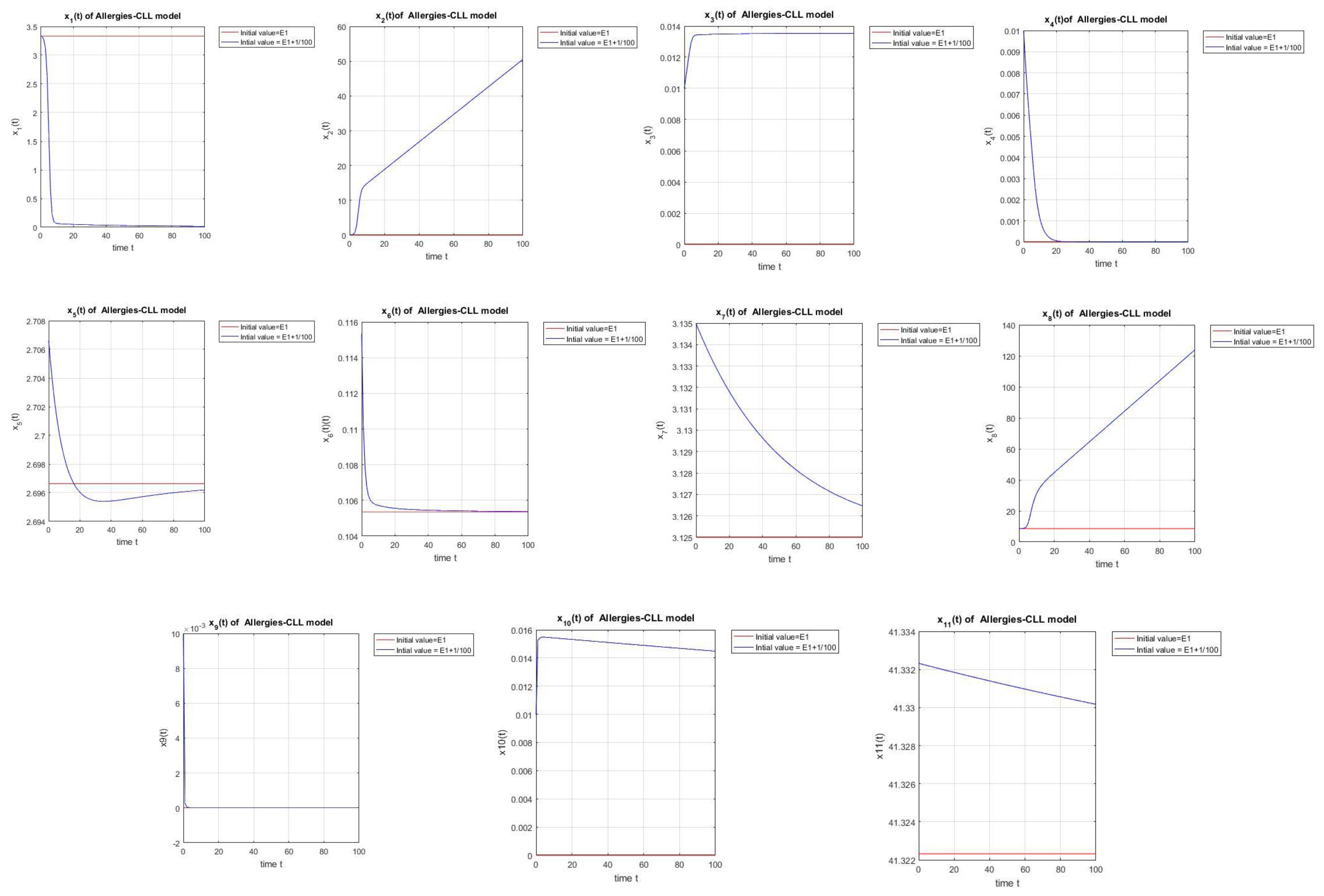
$E_1$ is an equilibrium point showing a successful chemoimmunotherapy without detection of allergic reactions, because the $Th1$ cell population dominates the $Th2$ cell population, as shown in Figure 1. When the stability for $E_1$ holds we will have successful therapy, and this shows that small quantities of allergens do not harm.

6.2. Numerical Simulations for $E_2$

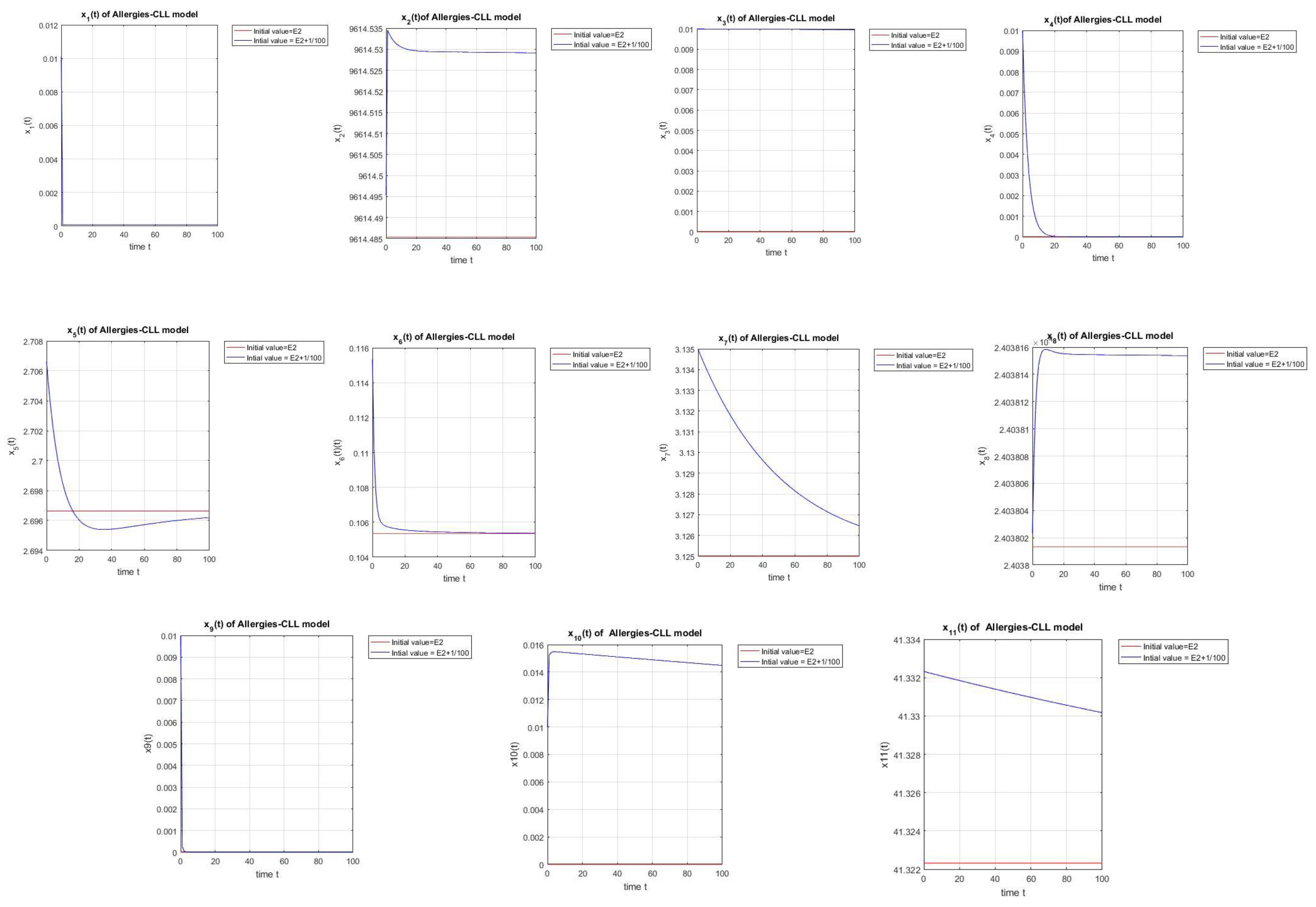
According to the simulations shown in Figure 2 starting with a desensitization dose of chemotherapy we will have successful chemoimmunotherapy without the detection of allergies even if we start with small values of $Th1$ cells, because the $Th1$ cell population will dominate the $Th2$ cell population.

7. Conclusions

Our paper presents a new model for cellular evolution in the case of chronic lymphocytic leukemia (CLL). We assumed that the treatment is with chlorambucil. As this drug has been proven to cause allergic reactions, we included the effects of desensitization. We also included an equation which captures the number of dead leukemic cells present in the body at any given time. We included this in order to monitor the risk of tumor lysis syndrome (TLS), which is caused by an abundance of leukemic cells dying in a short period of time.

The mathematical model which illustrates the complex interplay between the immune system, the presence of the leukemic cells and the effects of the treatment, consists of 11 delayed-differential equations, the dynamics of which are thoroughly described in the paper.

We have established qualitative properties of the solutions, including partial stability with respect to certain variables and the invariant set of positive initial data. By proving these properties, we have gained insights into the behavior of the system and its response to chemotherapy and allergic reactions.

Furthermore, numerical simulations have been conducted to complement the theoretical analysis. The simulations explore the interplay between the immune system’s function, the involvement of chemotherapy in cancer treatment, and the occurrence of allergic reactions due to the therapy. Numerical results obtained from the simulations have been presented.

Based on the provided information, it appears that the theoretical analysis shows that both equilibrium points $E_1$ and $E_2$ are not stable. The numerical computations align with this finding, confirming that both $E_1$ and $E_2$ are indeed not stable, contrary to the initial expectations. The numerical simulations further validate the theoretical results, reinforcing the conclusion that neither $E_1$ nor $E_2$ exhibit stability.

Theoretical results on partial stability have been derived under certain conditions. Specifically, we have shown that $E_1$ is partially stable with respect to variables $x_4$, $x_5$, $x_6$, $x_7$ and $x_9$, as well as with respect to the invariant manifold of solutions with positive components. Similarly, $E_2$ is partially stable with respect to variables $x_1$, $x_4$, $x_5$, $x_6$, $x_7$ and $x_9$, and with respect to the invariant manifold of solutions with positive components.

Additionally, the numerical simulations of equilibrium points $E_1$ and $E_2$ reinforce the theoretical findings on partial stability. The simulations demonstrate that both $E_1$ and $E_2$ exhibit partial stability with respect to the same variables that were studied and stated in the theoretical analysis. This consistency between the theoretical and numerical results further supports the validity of the partial stability conclusions for $E_1$ and $E_2$.

Furthermore, the numerical simulations of equilibrium points $E_1$ and $E_2$ provide valuable biological insights into the behavior of the system. The simulations shed light on the dynamics of chemoimmunotherapy and the occurrence of allergic reactions in patients with chronic lymphocytic leukemia (CLL).

The simulation results for $E_1$ reveal a scenario of successful chemoimmunotherapy without the detection of allergic reactions. This is attributed to the dominance of the Th1 cell population over the Th2 cell population, as observed in the simulation results. Even when starting with small quantities of allergens, the simulations demonstrate that the therapy remains effective, indicating that small amounts of allergens do not cause harm.

In the case of $E_2$, the simulations show a different outcome. Starting with a desensitization dose of chemotherapy, the simulations illustrate successful chemoimmunotherapy without the detection of allergies. Importantly, even with initially low levels of $Th1$ cells, the dominance of the $Th1$ cell population over the $Th2$ cell population is achieved, contributing to the positive treatment outcome.

These biological interpretations of the simulation results highlight the intricate interplay between the immune system, chemotherapy and allergic reactions. The simulations provide evidence that appropriate therapeutic strategies, such as desensitization dosing and the regulation of immune cell populations, can lead to successful treatment outcomes in CLL patients undergoing chemoimmunotherapy.

Overall, this study provides valuable insights into the dynamics of CLL patients undergoing chemotherapy and the impact of desensitization for chemotherapy-induced allergies. The combination of theoretical analysis and numerical simulations enhances our understanding of the system, and can potentially guide future clinical decision-making processes.

References

- Michor, F.; Beal, K. Improving Cancer Treatment via Mathematical Modeling: Surmounting the Challenges is Worth the Effort. Cell 2015, 163, 1059–1063. [Google Scholar] [CrossRef] [Green Version]
- Gammon, K. Mathematical modelling: Forecasting cancer. Nature 2012, 491, S66–S67. [Google Scholar] [CrossRef]
- Tambaro, F.P.; Wierda, W.G. Tumour lysis syndrome in patients with chronic lymphocytic leukaemia treated with BCL-2 inhibitors: Risk factors, prophylaxis, and treatment recommendations. Lancet Haematol. 2020, 7, e168–e176. [Google Scholar] [CrossRef]
- Fischer, K.; Al-Sawaf, O.; Hallek, M. Preventing and monitoring for tumor lysis syndrome and other toxicities of venetoclax during treatment of chronic lymphocytic leukemia. Hematology 2020, 2020, 357–362. [Google Scholar] [CrossRef]
- Guzev, E.; Luboshits, G.; Bunimovich-Mendrazitsky, S.; Firer, M.A. Experimental Validation of a Mathematical Model to Describe the Drug Cytotoxicity of Leukemic Cells. Symmetry 2021, 13, 1760. [Google Scholar] [CrossRef]
- Torricelli, R.; Kurer, S.B.; Kroner, T.; Wüthrich, B. Delayed allergic reaction to Chlorambucil (Leukeran). Case report and literature review. Schweiz. Med. Wochenschr. 1995, 125, 1870–1873. [Google Scholar]
- Levin, M.; Libster, D. Allergic reaction to chlorambucil in chronic lymphocytic leukemia presenting with fever and lymphadenopathy. Leuk. Lymphoma 2005, 46, 1195–1197. [Google Scholar] [CrossRef]
- Segel, L.A.; Fishman, M.A. Modeling immunotherapy for allergy. Bull. Math. Biol. 1996, 58, 1099–1121. [Google Scholar]
- Gross, F.; Behn, U. Mathematical modeling of allergy and specific immunotherapy: Th1, Th2 and Treg interactions. J. Theor. Biol. 2011, 269, 70–78. [Google Scholar] [CrossRef]
- Wu, G. Calculation of steady-state distribution delay between central and peripheral compartments in two-compartment models with infusion regimen. Eur. J. Drug Metab. Pharmacokinet. 2002, 27, 259–264. [Google Scholar] [CrossRef]
- Kareva, I.; Berezovskaya, F.; Karev, G. Mathematical model of a cytokine storm. bioRxiv, 2022; preprint. [Google Scholar] [CrossRef]
- Gubernatorova, E.O.; Gorshkova, E.A.; Namakanova, O.A.; Zvartsev, R.V.; Hidalgo, J.; Drutskaya, M.S.; Tumanov, A.V.; Nedospasov, S.A. Non-redundant Functions of IL-6 Produced by Macrophages and Dendritic Cells in Allergic Airway Inflammation. Front. Immunol. 2018, 9, 2718. [Google Scholar] [CrossRef] [Green Version]
- Colijn, C.; Mackey, M.C. A mathematical model of hematopoiesis—I. Periodic chronic myelogenous leukemia. J. Theor. Biol. 2005, 237, 117–132. [Google Scholar] [CrossRef]
- Gil, W.F.F.M.; Carvalho, T.; Mancera, P.F.A.; Rodrigues, D.S. A Mathematical Model on the Immune System Role in Achieving Better Outcomes of Cancer Chemotherapy. TEMA 2019, 20, 343–357. [Google Scholar] [CrossRef]
- Cooke, K.; Grossman, Z. Discrete Delay, Distribution Delay and Stability Switches. J. Math. Anal. Appl. 1982, 86, 592–627. [Google Scholar] [CrossRef] [Green Version]
- Kharitonov, V.L. Time-Delay Systems, Lyapunov Functionals and Matrices; Springer: Berlin/Heidelberg, Germany, 2013. [Google Scholar]
- Rumyantsev, V.; Vorotnikov, V.I. Foundations of Partial Stability and Control; Birkhouser: Nijnii Tagil, Russia, 2014. (In Russian) [Google Scholar]
- Aleksandrov, A.; Aleksandrova, E.; Zhabko, A.; Chen, Y. Partial stability analysis of some classes of nonlinear systems. Acta Math. Sci. 2017, 37B, 329–341. [Google Scholar] [CrossRef]
- Corduneanu, C. On partial stability for delay systems. Ann. Pol. Math. 1975, 29, 357–362. [Google Scholar] [CrossRef] [Green Version]
- Vorotnikov, V.I. Partial Stability and Control: The State-of-the-Art and Development Prospects; Ural State Technical University: Nizhni Tagil, Russia, 2003. [Google Scholar]
- Aristide, H. Differential Equation: Stability, Oscillations, Time-Lags; Academic Press: New York, NY, USA, 1966. [Google Scholar]
- Hatvani, L. On partial asymptotic stability and instability, I (Autonomous systems). Acta Sci. Math. 1983, 45, 219–231. [Google Scholar]
- Kim, P.; Lee, P.; Levy, D. A theory of immunodominance and adaptive regulation. Bull. Math. Biol. 2011, 73, 1645–1665. [Google Scholar] [CrossRef] [Green Version]
- Kogan, Y.; Agur, Z.; Elishmereni, M. A mathematical model for the immunotherapeutic control of the TH1/TH2 imbalance in melanoma. Discret. Contin. Dyn. Syst. Ser. B 2013, 18, 1017–1030. [Google Scholar] [CrossRef]
- Nazari, F.; Pearson, A.T.; Nor, J.E.; Jackson, T.L. A mathematical model for IL-6-mediated, stem cell driven tumor growth and targeted treatment. PLoS Comput. Biol. 2018, 14, e1005920. [Google Scholar] [CrossRef] [Green Version]
- Hong, T.; Xing, J.; Li, L.; Tyson, J.J. A Mathematical Model for the Reciprocal Differentiation of T Helper 17 Cells and Induced Regulatory T Cells. PLoS Comput. Biol. 2011, 7, e1002122. [Google Scholar] [CrossRef] [Green Version]
- Rădulescu, I.; Cândea, D.; Halanay, A. A study on stability and medical implications for a complex delay model for CML with cell competition and treatment. J. Theor. Biol. 2014, 363, 30–40. [Google Scholar] [CrossRef]
- Fouchet, D.; Regoes, R. A Population Dynamics Analysis of the Interaction between Adaptive Regulatory T Cells and Antigen Presenting Cells. PLoS ONE 2008, 3, e2306. [Google Scholar] [CrossRef] [Green Version]
- Rodrigues, D.; Mancera, P.; Carvalho, T.; Gonçalves, L. A mathematical model for chemoimmunotherapy of chronic lymphocytic leukemia. Appl. Math. Comput. 2019, 349, 118–133. [Google Scholar] [CrossRef] [Green Version]
Figure 1.
For a small disturbance in initial conditions near , the system exhibits partial stability, where = (3.3333, 0, 0, 0, 3.4164, 0.0334, 0.7813, 8.4167, 0, 0, 41.3223).
Figure 2.
Simulation of a small disturbance in initial conditions near . The equilibrium exhibits partial stability. = (, , 0, 0, 3.4164, 0.0334, 0.7813, , 0, 0, 41.3223).
Disclaimer/Publisher’s Note: The statements, opinions and data contained in all publications are solely those of the individual author(s) and contributor(s) and not of MDPI and/or the editor(s). MDPI and/or the editor(s) disclaim responsibility for any injury to people or property resulting from any ideas, methods, instructions or products referred to in the content. |
© 2023 by the authors. Licensee MDPI, Basel, Switzerland. This article is an open access article distributed under the terms and conditions of the Creative Commons Attribution (CC BY) license (https://creativecommons.org/licenses/by/4.0/).
Share and Cite
MDPI and ACS Style
Abdullah, R.; Badralexi, I.; Halanay, A. Stability Analysis in a New Model for Desensitization of Allergic Reactions Induced by Chemotherapy of Chronic Lymphocytic Leukemia. Mathematics 2023, 11, 3225. https://doi.org/10.3390/math11143225
AMA Style
Abdullah R, Badralexi I, Halanay A. Stability Analysis in a New Model for Desensitization of Allergic Reactions Induced by Chemotherapy of Chronic Lymphocytic Leukemia. Mathematics. 2023; 11(14):3225. https://doi.org/10.3390/math11143225
Chicago/Turabian StyleAbdullah, Rawan, Irina Badralexi, and Andrei Halanay. 2023. "Stability Analysis in a New Model for Desensitization of Allergic Reactions Induced by Chemotherapy of Chronic Lymphocytic Leukemia" Mathematics 11, no. 14: 3225. https://doi.org/10.3390/math11143225
Note that from the first issue of 2016, this journal uses article numbers instead of page numbers. See further details here.