Partial Eigenstructure Assignment for Linear Time-Invariant Systems via Dynamic Compensator

Abstract

This article studies the partial eigenstructure assignment (PEA) problem for a type of linear time-invariant (LTI) system. By introducing a dynamic output feedback controller, the closed-loop system is similar to a given arbitrary constant matrix, so the desired closed-loop eigenstructure can be obtained. Different from the normal eigenstructure assignment, only a part of the left and right generalized eigenvectors is assigned to the closed-loop system to remove complicated constraints, which reflects the partial eigenstructure assignment. Meanwhile, based on the solutions to the generalized Sylvester equations (GSEs), two arbitrary parameter matrices representing the degrees of freedom are presented to obtain the parametric form of the coefficient matrices of the dynamic compensator and the partial eigenvector matrices. Finally, an illustrative example and the simulation results prove the excellent effectiveness and feasibility of parametric method we proposed.

1. Introduction

Consider the following linear time-invariant (LTI) system

$$\left\{\begin{array}{cc}\hfill \dot{x}& =Ax+Bu,\hfill \\ \hfill y& =Cx,\hfill \end{array}\right.$$

(1)

where $x\in {\mathbb{R}}^n$, $u\in {\mathbb{R}}^r$ and $y\in {\mathbb{R}}^m$ are the state vector, input vector and output vector, respectively. $A, B, C$ are coefficient matrices with appropriate dimensions.

As an important problem in linear control systems design, eigenstructure assignment has attracted much attention among researchers in the last three decades, whether at home or abroad [1,2,3,4]. According to the theories of the linear system, its response is not only related to the eigenvalues of the system but also related to the corresponding eigenvectors [5,6]. Therefore, compared with the simple pole assignment, the eigenstructure assignment can grasp the dynamic performance of the system more accurately. Numerous successes based on the eigenstructure assignment theory have been achieved in previous years (see references in [7,8,9]).

Generally, we assign the whole set of right or left generalized eigenvectors into the closed-loop system, which is also called entire eigenstructure assignment. However, when the normality of the pair of right or left eigenvector matrices is abandoned, a large number of complicated constraints can be removed. In this situation, we only need to assign only a subset of left and right eigenvectors, not the whole set, which will reduce the computational load and make the design of the controller more economical and efficient. Due to this intriguing fact, the issue of partial eigenstructure assignment (PEA) arises. Some preliminary results of the PEA problem were given by Lu et al. and other authors in [10]. In this study, Lu et al. proposed a parametric solution and applied it to large-scale systems. Then, Duan et al. used the parametric method to solve the PEA problem of first-order normal systems and descriptor systems [11,12,13]. Furthermore, by using the degrees of freedom in the parameter matrix, Gu et al. extended the earlier results to high-order systems and further enhanced the system performance [14,15,16]. Meanwhile, Ouyang et al. also obtained a series of fruitful achievements for second-order vibration systems in [17,18,19]. They directly work on the second-order form and enable prior specification of the control matrix. Under these circumstances, it naturally results in the feedback gain matrices having a small norm solution. Additionally, there are also many positive results in different types of linear systems for the PEA problem (see references therein [20,21,22,23]). Of note, the above approach is for designing state feedback or static output feedback by the parametric or polynomial matrix method. Although they can solve this kind of problem well, it also inevitably has some drawbacks to some extent. On the one hand, due to the challenging working conditions, the state variables of the original system are frequently inaccessible in many practical applications. Based on this point, state feedback is sometimes difficult to achieve. On the other hand, because the static output feedback cannot arbitrarily assign to the poles of the closed-loop system, its control effect has great limitations. In order to address the shortcomings of the aforementioned techniques, we design a dynamic compensator, a form of dynamic output feedback controller. Gu and Zhang have performed excellent work on dynamic compensators in [24,25]. Therefore, the goal of our work is to fully utilize this type of dynamic compensator to address the issue raised in our paper.

For the system (1), we design the following dynamic compensator:

$$\left\{\begin{array}{cc}\hfill \dot{\xi }& =F\xi +My,\hfill \\ \hfill u& =P\xi +Qy,\hfill \end{array}\right.$$

(2)

where $\xi \in {\mathbb{R}}^p$ is the compensation vector. $F\in {\mathbb{R}}^{p\times p},M\in {\mathbb{R}}^{p\times m},P\in {\mathbb{R}}^{r\times p}$, and $Q\in {\mathbb{R}}^{r\times m}$ are the coefficient matrices of the dynamic compensator (2) to be determined in our paper. The closed-loop system with the aforementioned controller can be expressed as

$$\left[\begin{array}{c}\dot{x}\\ \dot{\xi }\end{array}\right]=A_c\left[\begin{array}{c}x\\ \xi \end{array}\right],$$

(3)

where

$$A_c=\left[\begin{array}{cc}A+BQC& BP\\ MC& F\end{array}\right].$$

According to the theory of linear systems, the comprehensive performance of the system (3) is totally determined by the closed-loop matrix $A_c$.

The main contribution of our work is designing a dynamic compensator and proposing a parametric method to solve the problem of PEA. The proposed method has the following features. Firstly, by letting the closed-loop system matrix be similar to a constant matrix with the desired eigenstructure, we establish a general parametric expression of the coefficient matrices of the dynamic compensator and other corresponding matrices to be solved. Secondly, through the above process, a subset of the left and right eigenvectors, not the whole set of eigenvectors, is assigned to the closed-loop system to reduce the large number of constraints, which makes the design of controller more economical and suitable for most of the practical applications. Finally, the system’s added performance is attained by fully utilizing the degrees of design flexibility in arbitrary parameters.

The sections that make up the majority of this article are as follows: In Section 2, we put forward some assumptions and notations needed in the text. Section 3 gives some preliminary results and the problem description to pave the way for the following sections. In Section 4 and Section 5, parametric solutions and a design algorithm are given to solve the main PEA problem in this paper. Meanwhile, the important role of arbitrary parameters in the controller design is discussed in Section 6. In Section 7, the efficiency of the suggested strategy is illustrated with an illustrative example and simulation comparison results. Finally, the work of this paper is summarized, and a conclusion is reached in Section 8.

2. Notations and Assumptions

Throughout this paper, the following assumptions, remark and notations in

Table 1. Notations and definitions.

Notations	Definition
${\mathbb{R}}^n$	set of all real vectors of dimension n
${\mathbb{C}}^n$	set of all complex vectors of dimension n
${\mathbb{C}}^{-}$	the points on the left-half s-plane
${\mathbb{R}}^{n\times m}$	set of all real matrices of dimension $n\times m$
$I_n$	the identity matrix with n dimensions
$\mathrm{rank}A$	the rank of the matrix A
$\det A$	the determinant of the matrix A
$\mathrm{eig}A$	all eigenvalues of the matrix A
${\left|\right|K\left|\right|}_2$	the Spectral norm of matrix K
$\mathrm{deg}A\left(s\right)$	the degree n of polynomial matrix $A\left(s\right)=A_0+s{A}_1+\cdots +s^n{A}_n$
$\mathrm{diag}({\lambda }_i,i=1,2,\dots ,m)$	the diagonal matrix with diagonal elements ${\lambda }_i$
$\mathrm{Im}\left({\lambda }_j^l\right)$	the imaginary part of ${\lambda }_j^l$

should be addressed to better solve our problem.

Assumption 1.

$\mathrm{rank}B=r$, $\mathrm{rank}C=m$.

Assumption 2.

$\mathrm{rank}\left[\begin{array}{cc}sI-A& B\end{array}\right]=\mathrm{rank}\left[\begin{array}{cc}sI-A^{\mathrm{T}}& C^{\mathrm{T}}\end{array}\right]=n$, $\forall s\in \mathbb{C}$.

Remark 1.

Assumption 1 above ensures the effective input signal and measurable output signal of the system, and Assumption 2 ensures the controllability and observability of the system.

3. Problem Description and Preliminary Results

In this paper, the work we conduct is to let the closed-loop matrix $A_c$ have the desired eigenstructure through the dynamic compensator (2). Specific details will be discussed later.

Usually, system (1) under the dynamic compensator (2) corresponds to the following static output feedback form:

$$\left\{\begin{array}{cc}\hfill \dot{X}& =\mathcal{A}X+\mathcal{B}U,\hfill \\ \hfill Y& =\mathcal{C}X,\hfill \end{array}\right.$$

(4)

where

$$\begin{array}{cc}\hfill X^{\mathrm{T}}& ={\left[\begin{array}{cc}{x}^{\mathrm{T}}& {\xi }^{\mathrm{T}}\end{array}\right]}^{\mathrm{T}},\hfill \\ \hfill U& =KY,\hfill \end{array}$$

(5)

and

$$\begin{array}{cc}\hfill \mathcal{A}& =\left[\begin{array}{cc}A& 0\\ 0& 0\end{array}\right],\mathcal{B}=\left[\begin{array}{cc}B& 0\\ 0& I_p\end{array}\right],\hfill \\ \hfill \mathcal{C}& =\left[\begin{array}{cc}C& 0\\ 0& I_p\end{array}\right],K=\left[\begin{array}{cc}Q& P\\ M& F\end{array}\right].\hfill \end{array}$$

(6)

The closed-loop system can be obtained by using the aforementioned relationships as

$$\dot{X}={\mathcal{A}}_{c}X,$$

(7)

where

$${\mathcal{A}}_c=\mathcal{A}+\mathcal{B}K\mathcal{C}.$$

In light of the given description, we thus provide the following lemma to begin our work.

Lemma 1.

Let $T,V\in {\mathbb{C}}^{(n+p)\times (n+p)}$ be the left and right generalized eigenvector matrices of the closed-loop system (3). Consider the following two generalized Sylvester equations

$$\begin{array}{cc}\hfill T^{\mathrm{T}}\mathcal{A}+G^{\mathrm{T}}\mathcal{C}& =\mathsf{\Gamma }{T}^{\mathrm{T}},\hfill \\ \hfill \mathcal{A}V+\mathcal{B}W& =V\mathsf{\Gamma },\hfill \end{array}$$

(8)

where

$$W=K\mathcal{C}V,G^{\mathrm{T}}=T^{\mathrm{T}}\mathcal{B}K,$$

and $\mathsf{\Gamma }\in {\mathbb{C}}^{(n+p)\times (n+p)}$ is an arbitrary matrix.

Partitioning the matrices T, V and W as

$$T=\left[\begin{array}{cc}{T}_a& T_b\end{array}\right],T_a\in {\mathbb{C}}^{(n+p)\times (n-m)},$$

(9)

$$V=\left[\begin{array}{cc}{V}_a& V_b\end{array}\right],V_a\in {\mathbb{C}}^{(n+p)\times (m+p)},$$

(10)

and

$$W=\left[\begin{array}{cc}{W}_a& W_b\end{array}\right],W_a\in {\mathbb{C}}^{(r+p)\times (m+p)}.$$

(11)

1. If the matrices $\mathcal{C}$ and $V_a$ hold

$$\det \left(\mathcal{C}{V}_a\right)\ne 0.$$

(12)

2. Then the output gain matrix K can be given by

$$K=W_a{\left(\mathcal{C}{V}_a\right)}^{-1}.$$

(13)

3.1. Partial Eigenvector Matrices

According to the above lemma, we first denote some matrices. Denote

$$\mathsf{\Lambda }=\left[\begin{array}{cc}{\mathsf{\Lambda }}_l& 0\\ 0& {\mathsf{\Lambda }}_r\end{array}\right],$$

(14)

where ${\mathsf{\Lambda }}_l\in {\mathbb{C}}^{(n-m)\times (n-m)}$, ${\mathsf{\Lambda }}_r\in {\mathbb{C}}^{(m+p)\times (m+p)}$ are two arbitrary given constant matrices. Meanwhile, denote $T\in {\mathbb{C}}^{(n+p)\times (n-m)}$, $V\in {\mathbb{C}}^{(n+p)\times (m+p)}$ as a part of left and right generalized eigenvector matrices, respectively, and $W\in {\mathbb{C}}^{(r+p)\times (m+p)}$ is a matrix corresponding to the GSE (8).

Remark 2.

For convenience, we still use the notations T, V and W to represent the left, right eigenvector and correlation matrices. However, they are no longer the entire matrices described in Lemma 1 but only a subset part of them. It can be easily observed that their dimensions are significantly reduced. Therefore, matrices T and V in this article are called partial eigenvector matrices.

In this paper, the goal is to let the closed-loop matrix ${\mathcal{A}}_c$ be similar to an arbitrary given constant matrix $\mathsf{\Lambda }$ in (14). In other words, we let one part of ${\mathcal{A}}_c$ be similar to ${\mathsf{\Lambda }}_l$ while the remaining part is similar to ${\mathsf{\Lambda }}_r$.

3.2. Problem Statement

Following the aforementioned preparation, the problem of the partial eigenstructure assignment via the dynamic compensator for a particular class of LTI systems is presented.

Problem 1.

Given the linear system (1) satisfying Assumptions 1 and 2. For two real given matrices ${\mathsf{\Lambda }}_l\in {\mathbb{R}}^{(n-m)\times (n-m)}$ and ${\mathsf{\Lambda }}_r\in {\mathbb{R}}^{(m+p)\times (m+p)}$, design and obtain all the coefficient matrices $F,M,P,Q$ of the dynamic compensator and all the partial eigenvector matrices $V\in {\mathbb{C}}^{(n+p)\times (m+p)}$, $T\in {\mathbb{C}}^{(n+p)\times (n-m)}$ satisfying the following equations:

$$T^{\mathrm{T}}V=0,$$

(15)

$$T^{\mathrm{T}}{\mathcal{A}}_{c}V=\left[\begin{array}{cc}{\mathsf{\Lambda }}_l& 0\\ 0& {\mathsf{\Lambda }}_r\end{array}\right].$$

(16)

With the transformation proposed in (4)–(7), Problem 1 can be transformed into the following Problem 2.

Problem 2.

Given the linear system (4) and two arbitrary constant matrices ${\mathsf{\Lambda }}_l,{\mathsf{\Lambda }}_r$ in (14), the left and right partial eigenvector matrices $T\in {\mathbb{C}}^{(n+p)\times (n-m)}$, $V\in {\mathbb{C}}^{(n+p)\times (m+p)}$ and the static output feedback gain matrix $K\in {\mathbb{R}}^{(r+p)\times (m+p)}$ satisfy

$$T^{\mathrm{T}}V=0,$$

(17)

$$\mathrm{rank}T=n-m,$$

(18)

$$\det \left(\mathcal{C}V\right)\ne 0,$$

(19)

and

$$T^{\mathrm{T}}{\mathcal{A}}_{c}V=\left[\begin{array}{cc}{\mathsf{\Lambda }}_l& 0\\ 0& {\mathsf{\Lambda }}_r\end{array}\right].$$

(20)

3.3. Preliminary Results

Before proposing the main solution regarding the problem, two pairs of polynomial matrices and right coprime factorization (RCF) are introduced.

Consider a pair of polynomial matrices

$$\left\{\begin{array}{cc}\hfill N\left(s\right)& =\sum _{i=0}^{{\omega }_r}{N}_i{s}^i,N_i\in {\mathbb{R}}^{n\times r},\hfill \\ \hfill D\left(s\right)& =\sum _{i=0}^{{\omega }_r}{D}_i{s}^i,D_i\in {\mathbb{R}}^{r\times r},\hfill \end{array}\right.$$

(21)

which are right comprime and satisfy

$${(sI-A)}^{-1}B=N\left(s\right)D^{-1}\left(s\right),$$

(22)

where ${\omega }_r$ = max$\{\mathrm{deg}\left(d_{ij}\left(s\right)\right),i=1,2,\dots ,r,j=1,2,\dots ,r\}$ when denoting $D\left(s\right)$ = ${\left[d_{ij}\left(s\right)\right]}_{r\times r}$.

Similarly, there also exists another pair of polynomial matrices

$$\left\{\begin{array}{cc}\hfill H\left(s\right)& =\sum _{i=0}^{{\omega }_l}{H}_i{s}^i,H_i\in {\mathbb{R}}^{n\times m},\hfill \\ \hfill L\left(s\right)& =\sum _{i=0}^{{\omega }_l}{L}_i{s}^i,L_i\in {\mathbb{R}}^{m\times m},\hfill \end{array}\right.$$

(23)

which are also right coprime and satisfy

$${(sI-A^{\mathrm{T}})}^{-1}{C}^{\mathrm{T}}=H\left(s\right)L^{-1}\left(s\right),$$

(24)

where ${\omega }_l=\max \{\mathrm{deg}\left(l_{ij}\left(s\right)\right),i=1,2,\dots ,m,j=1,2,\dots ,m\}$ when denoting $L\left(s\right)={\left[l_{ij}\left(s\right)\right]}_{m\times m}$.

Lemma 2.

Given the linear system (1) satisfying Assumptions 1 and 2, we have

$$\begin{array}{cc}\hfill \mathcal{N}\left(s\right)& =\left[\begin{array}{cc}0& N\left(s\right)\\ I_p& 0\end{array}\right],\mathcal{D}\left(s\right)=\left[\begin{array}{cc}0& D\left(s\right)\\ s{I}_p& 0\end{array}\right],\hfill \\ \hfill \mathcal{H}\left(s\right)& =\left[\begin{array}{cc}0& H\left(s\right)\\ I_p& 0\end{array}\right],\mathcal{L}\left(s\right)=\left[\begin{array}{cc}0& L\left(s\right)\\ s{I}_p& 0\end{array}\right],\hfill \end{array}$$

(25)

where

$$\left\{\begin{array}{cc}\hfill \mathcal{N}\left(s\right)& =\sum _{i=0}^{{\omega }_r}{\mathcal{N}}_i{s}^i,{\mathcal{N}}_i\in {\mathbb{R}}^{(n+p)\times (r+p)},\hfill \\ \hfill \mathcal{D}\left(s\right)& =\sum _{i=0}^{{\omega }_r}{\mathcal{D}}_i{s}^i,{\mathcal{D}}_i\in {\mathbb{R}}^{(r+p)\times (r+p)},\hfill \end{array}\right.$$

(26)

$$\left\{\begin{array}{cc}\hfill \mathcal{H}\left(s\right)& =\sum _{i=0}^{{\omega }_l}{\mathcal{H}}_i{s}^i,{\mathcal{H}}_i\in {\mathbb{R}}^{(n+p)\times (m+p)},\hfill \\ \hfill \mathcal{L}\left(s\right)& =\sum _{i=0}^{{\omega }_l}{\mathcal{H}}_i{s}^i,{\mathcal{L}}_i\in {\mathbb{R}}^{(m+p)\times (m+p)},\hfill \end{array}\right.$$

(27)

and

$$\left\{\begin{array}{cc}\hfill {(sI-\mathcal{A})}^{-1}\mathcal{B}& =\mathcal{N}\left(s\right){\mathcal{D}}^{-1}\left(s\right),\hfill \\ \hfill {(sI-{\mathcal{A}}^{\mathrm{T}})}^{-1}{\mathcal{C}}^{\mathrm{T}}& =\mathcal{H}\left(s\right){\mathcal{L}}^{-1}\left(s\right),\hfill \end{array}\right.$$

(28)

4. Parametric Solutions to Problem PEA

4.1. ${\mathsf{\Lambda }}_l$ and ${\mathsf{\Lambda }}_r$ Are Arbitrary

With the above description, a theorem regarding to Problems 1 and 2 can be given as follow.

Theorem 1.

Let $N\left(s\right),D\left(s\right),H\left(s\right),L\left(s\right)$ be two pairs of polynomial matrices satisfying RCF (22) (24), respectively. Additionally, $\mathcal{N}\left(s\right),\mathcal{D}\left(s\right),\mathcal{H}\left(s\right),\mathcal{L}\left(s\right)$ satisfy RCF (28).

(1) Problems 1 and 2 have a solution if and only if there exist two arbitrary parameter matrices $Z_l\in {\mathbb{C}}^{(m+p)\times (n-m)},Z_r\in {\mathbb{C}}^{(r+p)\times (m+p)}$ that satisfy the following condition:

$${\mathsf{\Lambda }}_{el}^{\mathrm{T}}\mathsf{\Psi }(Z_l,Z_r){\mathsf{\Lambda }}_{er}=0,$$

(29)

with

$${\mathsf{\Lambda }}_{el}=\left[\begin{array}{c}I\\ {\mathsf{\Lambda }}_l\\ ⋮\\ {\mathsf{\Lambda }}_l^{{\omega }_l}\end{array}\right],{\mathsf{\Lambda }}_{er}=\left[\begin{array}{c}I\\ {\mathsf{\Lambda }}_r\\ ⋮\\ {\mathsf{\Lambda }}_r^{{\omega }_r}\end{array}\right],$$

(30)

and

$$\mathsf{\Psi }(Z_l,Z_r)=\left[{\mathsf{\Psi }}_{ij}(Z_l,Z_r)\right],$$

(31)

where

$${\mathsf{\Psi }}_{ij}(Z_l,Z_r)=Z_l^{\mathrm{T}}{\mathcal{H}}_i^{\mathrm{T}}{\mathcal{N}}_j{Z}_r,i=1,2,\dots ,{\omega }_l;j=1,2,\dots ,{\omega }_r.$$

(32)

(2) When the above condition is met, all the partial eigenvector matrices $T,V$ in Equation (16) can be obtained as

$$\begin{array}{cc}\hfill T=\left[\begin{array}{c}{T}_0\\ T_1\end{array}\right]& =\sum _{i=0}^{{\omega }_l}{\mathcal{H}}_i{Z}_l{\left({\mathsf{\Lambda }}_l^{\mathrm{T}}\right)}^i=\sum _{i=0}^{{\omega }_l}{\mathcal{H}}_i\left[\begin{array}{c}{Z}_{l1}\\ Z_{l0}\end{array}\right]{\left({\mathsf{\Lambda }}_l^{\mathrm{T}}\right)}^i,\hfill \end{array}$$

(33)

with

$$\left\{\begin{array}{cc}\hfill T_0& =\sum _{i=0}^{{\omega }_l}{H}_i{Z}_{l0}{\left({\mathsf{\Lambda }}_l^{\mathrm{T}}\right)}^i,\hfill \\ \hfill T_1& =Z_{l1},\hfill \end{array}\right.$$

(34)

and

$$\begin{array}{cc}\hfill V=\left[\begin{array}{c}{V}_0\\ V_1\end{array}\right]& =\sum _{i=0}^{{\omega }_r}{\mathcal{N}}_i{Z}_r{\mathsf{\Lambda }}_r^i=\sum _{i=0}^{{\omega }_r}{\mathcal{N}}_i\left[\begin{array}{c}{Z}_{r1}\\ Z_{r0}\end{array}\right]{\mathsf{\Lambda }}_r^i,\hfill \end{array}$$

(35)

with

$$\left\{\begin{array}{cc}\hfill V_0& =\sum _{i=0}^{{\omega }_r}{N}_i{Z}_{r0}{\mathsf{\Lambda }}_r^i,\hfill \\ \hfill V_1& =Z_{r1},\hfill \end{array}\right.$$

(36)

where $Z_{l0}\in {\mathbb{C}}^{m\times (n-m)}$, $Z_{l1}\in {\mathbb{C}}^{p\times (n-m)}$, $Z_{r0}\in {\mathbb{C}}^{r\times (m+p)}$, $Z_{r1}\in {\mathbb{C}}^{p\times (m+p)}$ are arbitrary parameter matrices representing the degrees of freedom in the solutions satisfying the following constraints:

Constraint 1.

$\det \left(\widehat{C}V\right)\ne 0$.

Constraint 2.

$T_0^{\mathrm{T}}{V}_0+T_1^{\mathrm{T}}{V}_1=0$.

Constraint 3.

$\mathrm{rank}T=n-m$.

(3) With the above deduction, the output feedback gain matrix K can be calculated as

$$K=W{\left(\mathcal{C}V\right)}^{-1},$$

(37)

where

$$\begin{array}{cc}\hfill W& =\left[\begin{array}{c}{W}_0\\ W_1\end{array}\right]=\sum _{i=0}^{{\omega }_r}{\mathcal{D}}_i{Z}_r{\mathsf{\Lambda }}_r^i=\sum _{i=0}^{{\omega }_r}{\mathcal{D}}_i\left[\begin{array}{c}{Z}_{r1}\\ Z_{r0}\end{array}\right]{\mathsf{\Lambda }}_r^i,\hfill \end{array}$$

(38)

with

$$W_0=\sum _{i=0}^{{\omega }_r}{D}_i{Z}_{r0}{\mathsf{\Lambda }}_r^i,W_1=V_1{\mathsf{\Lambda }}_r.$$

(39)

Proof. 

Three parts make up the proof for this theorem.

Part 1 Derive the results in Equations (29)–(32).

Considering T and V in Equations (33) and (35), we have

$$T^{\mathrm{T}}=\sum _{i=0}^{{\omega }_l}{\mathsf{\Lambda }}_l^i{Z}_l^{\mathrm{T}}{\mathcal{H}}_i^{\mathrm{T}}=\left[\begin{array}{cccc}I& {\mathsf{\Lambda }}_l& \cdots & {\mathsf{\Lambda }}_l^{{\omega }_l}\end{array}\right]{\mathsf{\Psi }}_M^{\mathrm{T}}\left(Z_l\right)={\mathsf{\Lambda }}_{el}^{\mathrm{T}}{\mathsf{\Psi }}_M^{\mathrm{T}}\left(Z_l\right),$$

(40)

with

$${\mathsf{\Psi }}_M\left(Z_l\right)=\left[\begin{array}{cccc}{\mathcal{H}}_0{Z}_l& {\mathcal{H}}_1{Z}_l& \cdots & {\mathcal{H}}_{{\omega }_l}{Z}_l\end{array}\right],$$

(41)

and

$$V=\sum _{i=0}^{{\omega }_r}{\mathcal{N}}_i{Z}_r{\mathsf{\Lambda }}_r^i={\mathsf{\Psi }}_N\left(Z_r\right)\left[\begin{array}{c}I\\ {\mathsf{\Lambda }}_r\\ ⋮\\ {\mathsf{\Lambda }}_r^{{\omega }_r}\end{array}\right]={\mathsf{\Psi }}_N\left(Z_r\right){\mathsf{\Lambda }}_{er},$$

(42)

with

$${\mathsf{\Psi }}_N\left(Z_r\right)=\left[\begin{array}{cccc}{\mathcal{N}}_0{Z}_r& {\mathcal{N}}_1{Z}_r& \cdots & {\mathcal{N}}_{{\omega }_r}{Z}_r\end{array}\right].$$

(43)

Therefore, the Equation (15) can be rewritten as

$$\begin{array}{cc}\hfill T^{\mathrm{T}}V& =\left[\begin{array}{cccc}I& {\mathsf{\Lambda }}_l& \cdots & {\mathsf{\Lambda }}_l^{{\omega }_l}\end{array}\right]{\mathsf{\Psi }}_M^{\mathrm{T}}\left(Z_l\right){\mathsf{\Psi }}_N\left(Z_r\right)\left[\begin{array}{c}I\\ {\mathsf{\Lambda }}_r\\ ⋮\\ {\mathsf{\Lambda }}_r^{{\omega }_r}\end{array}\right]\hfill \\ \hfill & ={\mathsf{\Lambda }}_{el}^{\mathrm{T}}\mathsf{\Psi }(Z_l,Z_r){\mathsf{\Lambda }}_{er}=0.\hfill \end{array}$$

(44)

Obviously, ${\mathsf{\Psi }}_M^{\mathrm{T}}\left(Z_l\right){\mathsf{\Psi }}_N\left(Z_r\right)=\mathsf{\Psi }(Z_l,Z_r)$, and the elements of $\mathsf{\Psi }(Z_l,Z_r)$ have the result in Equation (32). Therefore, the proof of the first part is completed.

Part 2 Obtain matrices T, V and $W(\theta ,x)$ in Equations (33), (35) and (38).

Now, we consider Equations (7) and (20); two generalized Sylvester matrix equations can be given by

$$\begin{array}{cc}\hfill T^{\mathrm{T}}\mathcal{A}+G^{\mathrm{T}}\mathcal{C}& ={\mathsf{\Lambda }}_l{T}^{\mathrm{T}},\hfill \\ \hfill \mathcal{A}V+\mathcal{B}W& =V{\mathsf{\Lambda }}_r,\hfill \end{array}$$

(45)

where

$$W=K\mathcal{C}V,$$

(46)

$$G^{\mathrm{T}}=T^{\mathrm{T}}\mathcal{B}K.$$

(47)

Therefore, utilizing the solutions of the generalized Sylvester equation (see references [26,27]), the parametric expressions of matrices T, V, W can be obtained.

Meanwhile, considering Equations (25) and (33), we have

$$\begin{array}{cc}\hfill T& =\sum _{i=0}^{{\omega }_l}{\mathcal{H}}_i{Z}_l{\left({\mathsf{\Lambda }}_l^{\mathrm{T}}\right)}^i\hfill \\ \hfill & =\left[\begin{array}{cc}0& H_0\\ I_p& 0\end{array}\right]Z_l+\left[\begin{array}{cc}0& H_1\\ 0& 0\end{array}\right]Z_l{\mathsf{\Lambda }}_l^{\mathrm{T}}+\cdots +\left[\begin{array}{cc}0& H_{{\omega }_l}\\ 0& 0\end{array}\right]Z_l{\left({\mathsf{\Lambda }}_l^{\mathrm{T}}\right)}^{{\omega }_l}\hfill \\ \hfill & =\left[\begin{array}{cc}0& H_0\\ I_p& 0\end{array}\right]\left[\begin{array}{c}{Z}_{l1}\\ Z_{l0}\end{array}\right]+\left[\begin{array}{cc}0& H_1\\ 0& 0\end{array}\right]\left[\begin{array}{c}{Z}_{l1}\\ Z_{l0}\end{array}\right]{\mathsf{\Lambda }}_l^{\mathrm{T}}+\cdots +\left[\begin{array}{cc}0& H_{{\omega }_l}\\ 0& 0\end{array}\right]\left[\begin{array}{c}{Z}_{l1}\\ Z_{l0}\end{array}\right]{\left({\mathsf{\Lambda }}_l^{\mathrm{T}}\right)}^{{\omega }_l}\hfill \\ \hfill & =\left[\begin{array}{c}\sum _{i=0}^{{\omega }_l}{H}_i{Z}_{l0}{\left({\mathsf{\Lambda }}_l^{\mathrm{T}}\right)}^i\\ Z_{l1}\end{array}\right]=\left[\begin{array}{c}{T}_0\\ T_1\end{array}\right].\hfill \end{array}$$

(48)

Thus, Equation (34) holds. Similarly, Equation (36) also can be proved through the above process. We complete the proof of the second part.

Part 3 Derive the parametric expression of the output feedback gain matrix K in (37).

Firstly, by combining Equations (25) and (38), W can be expressed in the following form:

$$\begin{array}{cc}\hfill W& =\sum _{i=0}^{{\omega }_r}{\mathcal{D}}_i{Z}_r{\mathsf{\Lambda }}_r^i\hfill \\ \hfill & =\left[\begin{array}{cc}0& D_0\\ 0& 0\end{array}\right]Z_r+\left[\begin{array}{cc}0& D_1\\ I_p& 0\end{array}\right]Z_r{\mathsf{\Lambda }}_r+\cdots +\left[\begin{array}{cc}0& D_{{\omega }_r}\\ 0& 0\end{array}\right]Z_r{\mathsf{\Lambda }}_r^{{\omega }_r}\hfill \\ \hfill & =\left[\begin{array}{cc}0& D_0\\ 0& 0\end{array}\right]\left[\begin{array}{c}{Z}_{r1}\\ Z_{r0}\end{array}\right]+\left[\begin{array}{cc}0& D_1\\ I_p& 0\end{array}\right]\left[\begin{array}{c}{Z}_{r1}\\ Z_{r0}\end{array}\right]{\mathsf{\Lambda }}_r+\cdots +\left[\begin{array}{cc}0& D_{{\omega }_r}\\ 0& 0\end{array}\right]\left[\begin{array}{c}{Z}_{r1}\\ Z_{r0}\end{array}\right]{\mathsf{\Lambda }}_r^{{\omega }_r}\hfill \\ \hfill & =\left[\begin{array}{c}\sum _{i=0}^{{\omega }_r}{D}_i{Z}_{r0}{\mathsf{\Lambda }}_r^i\\ Z_{r1}{\mathsf{\Lambda }}_r\end{array}\right]=\left[\begin{array}{c}{W}_0\\ V_1{\mathsf{\Lambda }}_r\end{array}\right]=\left[\begin{array}{c}{W}_0\\ W_1\end{array}\right].\hfill \end{array}$$

(49)

Therefore, Equation (39) is proved.

Secondly, consider Equation (45); post-multiplying V and pre-multiplying $T^{\mathrm{T}}$, both sides, respectively, while using condition (17), we can obtain

$$\begin{array}{cc}\hfill T^{\mathrm{T}}\mathcal{A}V+T^{\mathrm{T}}\mathcal{B}W& =0,\hfill \\ \hfill T^{\mathrm{T}}\mathcal{A}V+G^{\mathrm{T}}\mathcal{C}V& =0.\hfill \end{array}$$

(50)

Comparing the above two equations, we obtain the following relation:

$$T^{\mathrm{T}}\mathcal{B}W=G^{\mathrm{T}}\mathcal{C}V.$$

(51)

Because Constraint 1 holds, the gain matrix K given by (37) obviously satisfies (46). While utilizing the above relation, we also have

$$\begin{array}{cc}\hfill T^{\mathrm{T}}\mathcal{B}K& =T^{\mathrm{T}}\mathcal{B}W{\left(\mathcal{C}V\right)}^{-1}\hfill \\ \hfill & =G^{\mathrm{T}}\mathcal{C}V{\left(\mathcal{C}V\right)}^{-1}\hfill \\ \hfill & =G^{\mathrm{T}},\hfill \end{array}$$

(52)

which illustrates that the output feedback gain matrix K provided by (37) also satisfies (47).

The uniqueness of the output feedback gain matrix simultaneously satisfying Equations (46) and (47) directly reveals the fact that Equation (46) has a unique solution under Constraint 1. Hence, the proof of this part is finished.

To sum up, we completed the whole proof of Theorem 1.  □

4.2. ${\mathsf{\Lambda }}_l$ and ${\mathsf{\Lambda }}_r$ Are Two Diagonal Matrices

The diagonal matrix has similar properties to the non-defective matrix. To the best of our knowledge, the eigenvalues of a non-defective matrix have a lower sensitivity to changes in the parameters of the coefficient matrix. Hence, in many applications, matrices ${\mathsf{\Lambda }}_l$ and ${\mathsf{\Lambda }}_r$ have a diagonal form, that is,

$${\mathsf{\Lambda }}_r=\mathrm{diag}({\lambda }_i,i=1,2,\dots ,m+p),$$

(53)

and

$${\mathsf{\Lambda }}_l=\mathrm{diag}({\lambda }_j,j=1,2,\dots ,n-m),$$

(54)

where ${\lambda }_i,i=1,2,\dots ,m+p$ and ${\lambda }_j,j=1,2,\dots ,n-m$ are eigenvalues to be assigned. In this situation, matrices T, V, and W can be written in the following forms:

$$\left\{\begin{array}{cc}\hfill V& =\left[\begin{array}{cccc}{v}_1& v_2& \cdots & v_{m+p}\end{array}\right],\hfill \\ \hfill v_i& =\left[\begin{array}{c}{v}_{0i}\\ v_{1i}\end{array}\right]=\mathcal{N}\left({\lambda }_i\right)z_i^r=\mathcal{N}\left({\lambda }_i\right)\left[\begin{array}{c}{z}_i^{r1}\\ z_i^{r0}\end{array}\right],\hfill \\ \hfill v_{0i}& =N\left({\lambda }_i\right)z_i^{r0},v_{1i}=z_i^{r1},i=1,2,\dots ,m+p,\hfill \end{array}\right.$$

(55)

$$\left\{\begin{array}{cc}\hfill T& =\left[\begin{array}{cccc}{t}_1& t_2& \cdots & t_{n-m}\end{array}\right],\hfill \\ \hfill t_j& =\left[\begin{array}{c}{t}_{0j}\\ t_{1j}\end{array}\right]=\mathcal{H}\left({\lambda }_j\right)z_j^l=\mathcal{H}\left({\lambda }_j\right)\left[\begin{array}{c}{z}_j^{l1}\\ z_j^{l0}\end{array}\right],\hfill \\ \hfill t_{0j}& =H\left({\lambda }_j\right)z_j^{l0},t_{1j}=z_j^{l1},j=1,2,\dots ,n-m,\hfill \end{array}\right.$$

(56)

$$\left\{\begin{array}{cc}\hfill W& =\left[\begin{array}{cccc}{w}_1& w_2& \cdots & w_{m+p}\end{array}\right],\hfill \\ \hfill w_i& =\left[\begin{array}{c}{w}_i^0\\ w_i^1\end{array}\right]=\mathcal{D}\left({\lambda }_i\right)z_i^r=\mathcal{D}\left({\lambda }_i\right)\left[\begin{array}{c}{z}_i^{r1}\\ z_i^{r0}\end{array}\right],\hfill \\ \hfill w_i^0& =D\left({\lambda }_i\right)z_i^{r0},w_i^1={\lambda }_i{v}_{1i},i=1,2,\dots ,m+p,\hfill \end{array}\right.$$

(57)

with

$$\begin{array}{cc}\hfill Z_r& =\left[\begin{array}{cccc}{z}_1^r& z_2^r& \cdots & z_{m+p}^r\end{array}\right],\hfill \\ \hfill Z_l& =\left[\begin{array}{cccc}{z}_1^l& z_2^l& \cdots & z_{n-m}^l\end{array}\right],\hfill \end{array}$$

(58)

and $z_i^{r0}\in {\mathbb{C}}^r$, $z_i^{r1}\in {\mathbb{C}}^p$, $i=1,2,\cdots ,m+p$, $z_j^{l0}\in {\mathbb{C}}^m$, $z_j^{l1}\in {\mathbb{C}}^p$, $j=1,2,\cdots ,n-m$ represent three degrees of freedom in the solution.

Based on the above description, we give another theorem to address Problems 1 and 2.

Theorem 2.

Let $N\left(s\right),D\left(s\right),H\left(s\right),L\left(s\right)$ be two pairs of polynomial matrices satisfying RCF (22) (24), respectively. Additionally, $\mathcal{N}\left(s\right),\mathcal{D}\left(s\right),\mathcal{H}\left(s\right),\mathcal{L}\left(s\right)$ satisfy RCF (28).

(1) Problems 1 and 2 have a solution if and only if there exist two groups of parameter vectors $z_i^r\in {\mathbb{C}}^{r+p}$, $z_j^l\in {\mathbb{C}}^{m+p}$, satisfying the relation

$$\begin{array}{cc}\hfill {\left(z_j^l\right)}^{\mathrm{T}}{\mathcal{H}}^{\mathrm{T}}\left({\lambda }_j^l\right)\mathcal{N}\left({\lambda }_i^r\right)z_i^r=0,i& =1,2,\dots ,m+p,\hfill \\ \hfill j& =1,2,\dots ,n-m.\hfill \end{array}$$

(59)

and the following constraints:

Constraint 4.

${\left(z_j^{l0}\right)}^{\mathrm{T}}{H}^{\mathrm{T}}\left({\lambda }_j\right)N\left({\lambda }_i\right)z_i^{r0}+{\left(z_j^{l1}\right)}^{\mathrm{T}}{z}_i^{r1}=0,i=1,2,\cdots ,m+p;j=1,2,\cdots ,n-m$.

Constraint 5.

$\det \left(\mathcal{C}V({\lambda }_i,z_i^r)\right)\ne 0,i=1,2,\cdots ,m+p$.

Constraint 6.

$z_j^l=z_k^{-l}$ if ${\lambda }_j^l={\lambda }_k^{-l}$, $\mathrm{Im}\left({\lambda }_j^l\right)\ne 0,j,k=1,2,\dots ,n-m$.

Constraint 7.

$z_i^r=z_k^{-r}$ if ${\lambda }_i^r={\lambda }_k^{-r}$, $\mathrm{Im}\left({\lambda }_i^r\right)\ne 0,i,k=1,2,\dots ,m+p$.

(2) When the above relation and constraints are satisfied, all the parametric solutions of the output feedback gain matrix K can be obtained as Equation (37), and the matrices $T,V$ in (33)–(36) and W in (38)–(39) can be parametrized by columns as (55)–(57).

Proof. 

When the matrices ${\mathsf{\Lambda }}_l$ and ${\mathsf{\Lambda }}_r$ are chosen as the diagonal form of (53) and (54), matrices T, V, and W can be the form of columns given by Equations (55)–(57), respectively.

Note that

$$\begin{array}{cc}\hfill T^{\mathrm{T}}V& =\left[\begin{array}{c}{\left(z_1^l\right)}^{\mathrm{T}}{\mathcal{H}}^{\mathrm{T}}\left({\lambda }_1^l\right)\\ {\left(z_2^l\right)}^{\mathrm{T}}{\mathcal{H}}^{\mathrm{T}}\left({\lambda }_2^l\right)\\ ⋮\\ {\left(z_{n-m}^l\right)}^{\mathrm{T}}{\mathcal{H}}^{\mathrm{T}}\left({\lambda }_{n-m}^l\right)\end{array}\right]\left[\begin{array}{cccc}\mathcal{N}\left({\lambda }_1^r\right)z_1^r& \mathcal{N}\left({\lambda }_2^r\right)z_2^r& \cdots & \mathcal{N}\left({\lambda }_{m+p}^r\right)z_{m+p}^r\end{array}\right]\hfill \\ \hfill & ={\left[\begin{array}{c}{\left(z_j^l\right)}^{\mathrm{T}}{\mathcal{H}}^{\mathrm{T}}\left({\lambda }_j^l\right)\mathcal{N}\left({\lambda }_i^r\right)z_i^r\end{array}\right]}_{(n-m)\times (m+p)}=0,\hfill \end{array}$$

(60)

which is equivalent to Equation (59). Therefore, we can easily prove the results of this theorem.  □

5. Design Algorithm for Problem PEA

In light of the aforementioned theorems, we provide a design algorithm step to address Problem PEA.

Step 1 Obtain two pairs of coprime matrices $N\left(s\right)$, $D\left(s\right)$, $H\left(s\right)$, $L\left(s\right)$.

In the previous section, we mentioned that Problem PEA in this article can be transformed into the solutions of two Sylvester equations. In addition to the parameter matrices $Z_l$ and $Z_r$ that we choose arbitrarily, the most important point is to find two sets of right coprime polynomial matrices that satisfy Equations (22) and (24)

Step 2 Choose an expected closed-loop eigenstructure.

The primary task of the control system design is to ensure the stability of the closed-loop system (7). To achieve the above goal, the matrices ${\mathsf{\Lambda }}_l$ and ${\mathsf{\Lambda }}_r$ are usually required to be two Hurwitz matrices [28,29], which means

$$\mathrm{eig}\left({\mathsf{\Lambda }}_l\right)\in {\mathbb{C}}^{-},\mathrm{eig}\left({\mathsf{\Lambda }}_r\right)\in {\mathbb{C}}^{-}.$$

(61)

Step 3 Select proper parameters.

In this paper, the arbitrary parameter matrices $Z_r$ and $Z_l$ play an important role in the design of the controller. Specifically, the above two matrices provide all the degrees of freedom in the system design. By selecting the appropriate arbitrary parameters satisfying the constraints in this article, the additional design requirements of the system can be well met.

Step 4 Compute the partial eigenvector matrices T, V and other corresponding matrices.

Based on the solutions for matrices T, V, and W given in Equations (33)–(39) or (55)–(57), compute the above matrices with the selected parameters given in Step 3.

Step 5 Obtain the parametric form of the output feedback controller matrix K.

Based on the solutions in Step 4, the static output feedback gain matrix K can be solved by Equation (37). Therefore, utilizing the relation in Equation (6), the coefficient matrices F, M, P, and Q of the dynamic compensator (2) can be obtained.

6. Utilizing the Degrees of Freedom in Parameters

Up to now, we recall the fact that all the solutions of the parametric method are closely related to the arbitrary matrices $Z_l,Z_r$, that is,

$$\left\{\begin{array}{cc}\hfill T& =T(Z_l,{\mathsf{\Lambda }}_l),\hfill \\ \hfill V& =V(Z_r,{\mathsf{\Lambda }}_r),\hfill \\ \hfill W& =W(Z_r,{\mathsf{\Lambda }}_r),\hfill \\ \hfill K& =K(Z_r,{\mathsf{\Lambda }}_r),\hfill \end{array}\right.$$

(62)

if the two matrices ${\mathsf{\Lambda }}_r,{\mathsf{\Lambda }}_l$ are determined in advance, then all the solutions depend on the values of arbitrary parameters. The fundamental benefit of our approach is evident here. The degrees of freedom can be greatly improved, that is, the desired control law can be achieved by choosing different parameter matrices.

Based on the above discussion, we establish two indices and then implement the optimization.

• Low control gain

The low control gain index is well known to have a significant influence on the design of the controllers. The low control gain can reduce the series amplifier and make it difficult to achieve self-oscillation, which has a significant practical impact. Consequently, we decide on the following index as

$$J_1\left(Z_r\right)=\frac{1}{2}\left|\right|P\left(Z_r\right){\left|\right|}_2+\frac{1}{2}\left|\right|Q\left(Z_r\right){\left|\right|}_2.$$

(63)

• Low compensation gain

From Equation (2), we can find that the consumption of energy depends on the compensation vector $\xi$. To reduce the energy loss and minimize the energy consumption during the transient process, we choose the following index as

$$J_2\left(Z_r\right)=\frac{1}{2}\left|\right|F\left(Z_r\right){\left|\right|}_2+\frac{1}{2}\left|\right|M\left(Z_r\right){\left|\right|}_2.$$

(64)

Hence, a synthetic object function that describes the system performance is given by

$$J\left(Z_r\right)=J_1\left(Z_r\right)+J_2\left(Z_r\right).$$

(65)

Based on the above preparation, an optimization problem can be defined as

$$\left\{\begin{array}{c}\min J\left(Z_r\right)\hfill \\ \mathrm{s}.\mathrm{t}.\left(17\right),\left(18\right),\left(19\right),\left(21\right).\hfill \end{array}\right.$$

(66)

Of note, in this problem, the arbitrary matrix $Z_r$ serves as the optimization variable. Hence, the desired index can be optimized and achieved by utilizing the degrees of freedom in $Z_r$. After that, another group of parameter matrix $Z_l$ can be obtained under the relation in (17).

Remark 3.

It is nearly impossible or even impossible to satisfy several sophisticated restrictions in many real applications. In the entire eigenstructure assignment by output feedback, the condition (15) is $T^{\mathrm{T}}V=I$, which indicates that the system needs to solve the number of $(n+p)\times (n+p)$ equations [30,31]. However, when we abandon a part of the left and right eigenvectors for the partial eigenstructure assignment, the constraint becomes (15) and the number of constraints is reduced to $(n-m)\times (m+p)$, which greatly facilitates the design of the controller and makes the design process more straightforward, affordable, and efficient.

7. An Illustrative Example

In this example, we make a simple comparison with Liu and R. J. Patton in [32] to better illustrate that we can not only obtain the expected eigenstructure of the closed-loop system but also realize the additional design requirements of the closed-loop system by making full use of the degrees of freedom provided by the arbitrary parameter matrices $Z_r$ and $Z_l$ in this method.

7.1. System Description

Consider the following coefficient matrices for a linear system with the form (1)

$$A=\left[\begin{array}{ccc}0& 1& 0\\ 1& 1& 0\\ -1& 0& 0\end{array}\right],B={\left[\begin{array}{ccc}0& 1& 0\end{array}\right]}^{\mathrm{T}},C=\left[\begin{array}{ccc}1& 0& 0\\ 0& 0& 1\end{array}\right],$$

Before we analyze and design this system, it is simple to confirm that

$$\mathrm{rank}B=1,\mathrm{rank}C=2,$$

$$\begin{array}{cc}\hfill & \mathrm{rank}\left[\begin{array}{cc}sI-A& B\end{array}\right]=\mathrm{rank}\left[\begin{array}{cccc}s& -1& 0& 0\\ -1& s-1& 0& 1\\ 1& 0& s& 0\end{array}\right]=3,\forall s\in \mathbb{C}\hfill \\ \hfill & \mathrm{rank}\left[\begin{array}{cc}sI-A^{\mathrm{T}}& C^{\mathrm{T}}\end{array}\right]=\mathrm{rank}\left[\begin{array}{ccccc}s& -1& 1& 1& 0\\ -1& s-1& 0& 0& 0\\ 0& 0& s& 0& 1\end{array}\right]=3,\forall s\in \mathbb{C}.\hfill \end{array}$$

Therefore, Assumptions 1 and 2 hold. Meanwhile, we can easily deduce two RCFs satisfying Equations (22) and (24):

$$\left\{\begin{array}{cc}\hfill N\left(s\right)& =\left[\begin{array}{c}-s\\ -s^2\\ 1\end{array}\right],\hfill \\ \hfill D\left(s\right)& =-s^3+s^2+s,\hfill \end{array}\right.\left\{\begin{array}{cc}\hfill H\left(s\right)& =\left[\begin{array}{cc}0& s-1\\ 0& 1\\ 1& -s^2+s+1\end{array}\right],\hfill \\ \hfill L\left(s\right)& =\left[\begin{array}{cc}1& 0\\ s& -s^3+s^2+s\end{array}\right].\hfill \end{array}\right.$$

Letting $p=1$, we design a dynamic compensator in the form of Equation (2) and choose two diagonal matrices with the desired closed-loop eigenvalues

$${\mathsf{\Lambda }}_l=\mathrm{diag}\{-1\},{\mathsf{\Lambda }}_r=\mathrm{diag}\{-1.5,-3,-6.5\}.$$

(67)

Meanwhile, denote two arbitrary matrices $Z_r$ and $Z_l$ as

$$Z_r=\left[\begin{array}{c}{Z}_{r1}\\ Z_{r0}\end{array}\right]=\left[\begin{array}{ccc}{\alpha }_{11}& {\alpha }_{12}& {\alpha }_{13}\\ {\alpha }_{21}& {\alpha }_{22}& {\alpha }_{23}\end{array}\right],Z_l=\left[\begin{array}{c}{Z}_{l1}\\ Z_{l0}\end{array}\right]=\left[\begin{array}{c}{\beta }_1\\ {\beta }_2\\ {\beta }_3\end{array}\right],$$

(68)

then condition (15) can be solved based on solutions (55)–(58):

$${\left[\begin{array}{c}{\alpha }_{11}{\beta }_1+{\alpha }_{21}{\beta }_2+(-{\lambda }_1^{r^2}+{\lambda }_1^r-{\lambda }_1^r{\lambda }_l-{\lambda }_l^2+{\lambda }_l+1){\alpha }_{21}{\beta }_3\\ {\alpha }_{12}{\beta }_1+{\alpha }_{22}{\beta }_2+(-{\lambda }_2^{r^2}+{\lambda }_2^r-{\lambda }_2^r{\lambda }_l-{\lambda }_l^2+{\lambda }_l+1){\alpha }_{22}{\beta }_3\\ {\alpha }_{13}{\beta }_1+{\alpha }_{23}{\beta }_2+(-{\lambda }_3^{r^2}+{\lambda }_3^r-{\lambda }_3^r{\lambda }_l-{\lambda }_l^2+{\lambda }_l+1){\alpha }_{23}{\beta }_3\end{array}\right]}^{\mathrm{T}}=0,$$

(69)

where ${\alpha }_{ij},{\beta }_i,i,j=1,2,3$, are some arbitrary real scalars, and ${\lambda }_l$ and ${\lambda }_i^r,i=1,2,3$ are the eigenvalues of the closed-loop system pre-determined in (67).

7.2. Non-Optimized Solution

Considering the arbitrary parameters in (68) and (69), particularly choose the values as follows:

$$Z_r=\left[\begin{array}{ccc}5.25& 15& 55.25\\ 1& 1& 1\end{array}\right],Z_l={\left[\begin{array}{ccc}1& 1& 1\end{array}\right]}^{\mathrm{T}},$$

(70)

then based on the solutions in (53)–(58), we have

$$T_0=\left[\begin{array}{c}-2\\ 1\\ 0\end{array}\right],V_0=\left[\begin{array}{ccc}1.5& 3& 6.5\\ -2.25& -9& -42.25\\ 1& 1& 1\end{array}\right],T_1=\left[\begin{array}{c}1\end{array}\right],V_1={\left[\begin{array}{c}5.25\\ 15\\ 55.25\end{array}\right]}^{\mathrm{T}},$$

and

$$W_0=\left[\begin{array}{ccc}4.125& 33& 310.375\end{array}\right],W_1=\left[\begin{array}{ccc}-7.875& -45& -359.125\end{array}\right].$$

With the above solutions and based on Equation (37), the output feedback gain matrix K can be obtained as

$$K=\left[\begin{array}{ccc}-58.75& 29.25& 12\\ 59.75& -29.25& -13\end{array}\right],$$

(71)

which means

$$\begin{array}{cc}\hfill Q& =\left[\begin{array}{cc}-58.75& 29.25\end{array}\right],P=\left[\begin{array}{c}12\end{array}\right],\hfill \\ \hfill M& =\left[\begin{array}{cc}59.75& -29.25\end{array}\right],F=\left[\begin{array}{c}-13\end{array}\right].\hfill \end{array}$$

(72)

With the controller (71) or (72), the closed-loop system can be implemented as

$$\left[\begin{array}{c}\dot{x}\\ \dot{\xi }\end{array}\right]=\left[\begin{array}{cccc}0& 1& 0& 0\\ -57.75& 1& 29.25& 12\\ -1& 0& 0& 0\\ 59.75& 0& -29.25& -13\end{array}\right]\left[\begin{array}{c}x\\ \xi \end{array}\right].$$

(73)

7.3. Optimized Solution

Consider the optimization problem in (66). Choose the initial values in (70), then the optimized parameters can be obtained by using the fmincon function (Equation (69)) in the MATLAB Optimization Toolbox${}^{\circledR }$:

$$Z_r=\left[\begin{array}{ccc}2.5346& 16.6276& 50.2855\\ 0.7157& 2.0781& 1.9038\end{array}\right],Z_l=\left[\begin{array}{c}5.5261\\ -3.7696\\ 2.5279\end{array}\right],$$

we have the following optimized solution

$$\begin{array}{cc}\hfill T_0& =\left[\begin{array}{c}-5.0559\\ 2.52779\\ -6.2976\end{array}\right],V_0=\left[\begin{array}{ccc}1.0736& 6.23428& 12.3744\\ -1.6104& -18.7028& -80.4338\\ 0.7157& 2.0781& 1.9038\end{array}\right],\hfill \\ \hfill T_1& =\left[\begin{array}{c}5.5261\end{array}\right],V_1=\left[\begin{array}{ccc}2.5346& 16.6276& 50.2855\end{array}\right],\hfill \end{array}$$

and

$$W_0=\left[\begin{array}{ccc}2.9524& 68.5771& 590.8794\end{array}\right],W_1=\left[\begin{array}{ccc}-3.8018& -49.8828& -326.8559\end{array}\right].$$

With the above solutions and based on Equation (37), the output feedback gain matrix K can be obtained as

$$K=\left[\begin{array}{ccc}-58.75& -0.6443& 26.2323\\ 26.1931& 1.4344& -13\end{array}\right],$$

(74)

which means

$$\begin{array}{cc}\hfill Q& =\left[\begin{array}{cc}-58.75& -0.6443\end{array}\right],P=\left[\begin{array}{c}26.2323\end{array}\right],\hfill \\ \hfill M& =\left[\begin{array}{cc}26.1931& 1.4344\end{array}\right],F=\left[\begin{array}{c}-13\end{array}\right].\hfill \end{array}$$

(75)

With the controller (74) or (75), the closed-loop system can be implemented as

$$\left[\begin{array}{c}\dot{x}\\ \dot{\xi }\end{array}\right]=\left[\begin{array}{cccc}0& 1& 0& 0\\ -57.75& 1& -0.6443& 26.2323\\ -1& 0& 0& 0\\ 26.1931& 0& 1.4343& -13\end{array}\right]\left[\begin{array}{c}x\\ \xi \end{array}\right].$$

(76)

7.4. Simulation Results and Comparison

In order to more clearly illustrate the benefit of the parametric method, the following simulation results and comparison are given.

Make the following initial value selections:

$$\left\{\begin{array}{cc}\hfill x\left(0\right)& ={\left[\begin{array}{ccc}1& 1& 1.5\end{array}\right]}^{\mathrm{T}},\hfill \\ \hfill \xi \left(0\right)& ={\left[\begin{array}{c}2\end{array}\right]}^{\mathrm{T}},\hfill \end{array}\right.$$

then the simulation results are shown in the following Figure 1, Figure 2, Figure 3, Figure 4 and Figure 5 and Table 1,

Table 2. Comparison of the closed-loop eigenvalues between three solutions.

Solutions	Closed-Loop Eigenvalues
Liu et al. [32]	−0.99979784, −1.49975243, −3.00067144, −6.49977829
Non-optimized solution	−1.00000000, −1.49999999, −3.00000000, −6.49999999
Optimized solution	−0.99999999, −1.50000000, −2.99999999, −6.50000000

,

Table 3. Comparison of the indices between three solutions.

Index	Value
	${\mathit{J}}_{\mathbf{1}}$	${\mathit{J}}_{\mathbf{2}}$	$\mathit{J}$
Liu et al. [32]	111.0955	54.9084	166.0039
Non-optimized solution	39.7627	38.8143	78.5770
Optimized solution	19.6102	42.4929	62.1091

and

Table 4. Comparison of the amplitude between three solutions.

Maximal Amplitude	Value(m)
	${\mathit{x}}_{\mathbf{1}}$	${\mathit{x}}_{\mathbf{2}}$	${\mathit{x}}_{\mathbf{3}}$	$\mathit{\xi }$
Liu et al. [32]	2.125	4.109	0.580	14.200
Non-optimized solution	1.327	1.127	0.048	3.853
Optimized solution	1.101	0.746	≈0	2.336

.

We analyze the above simulation results from the following three aspects:

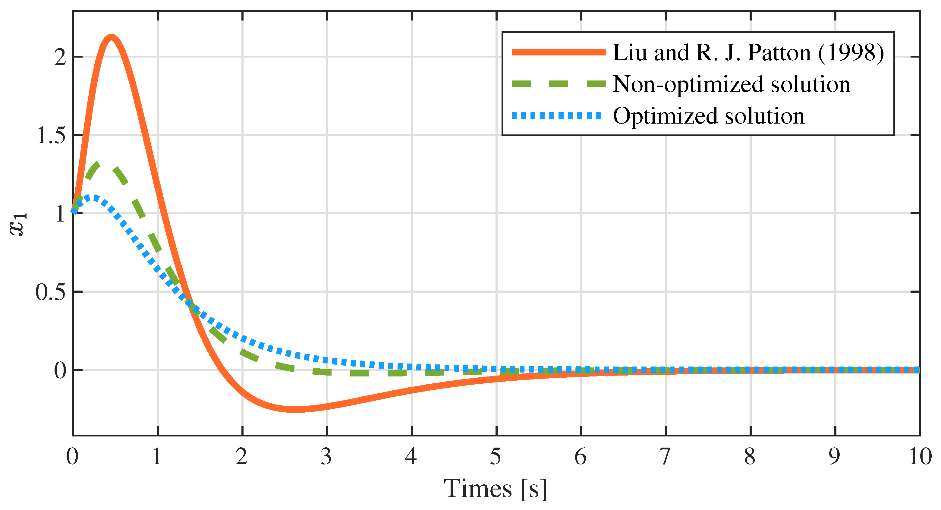
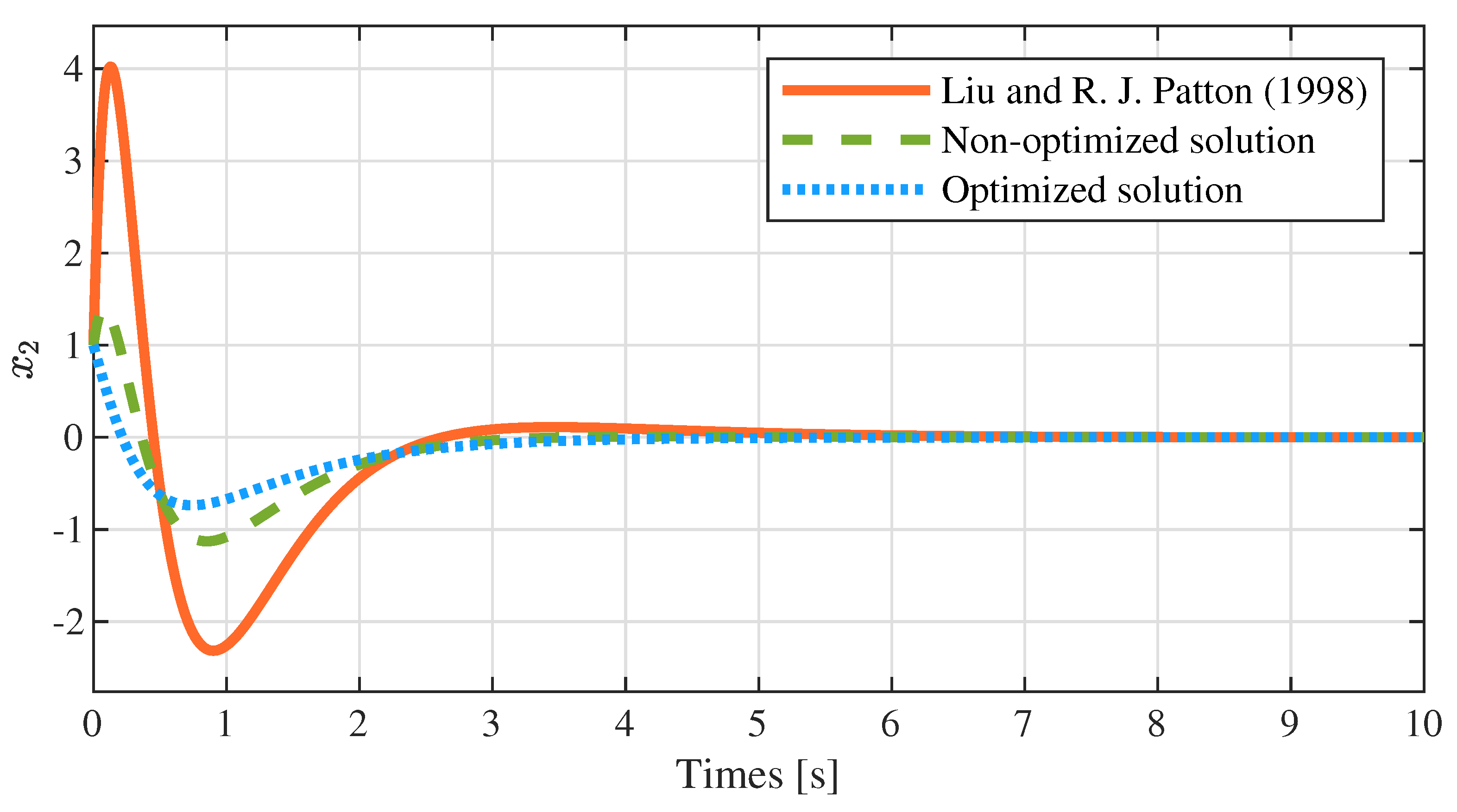
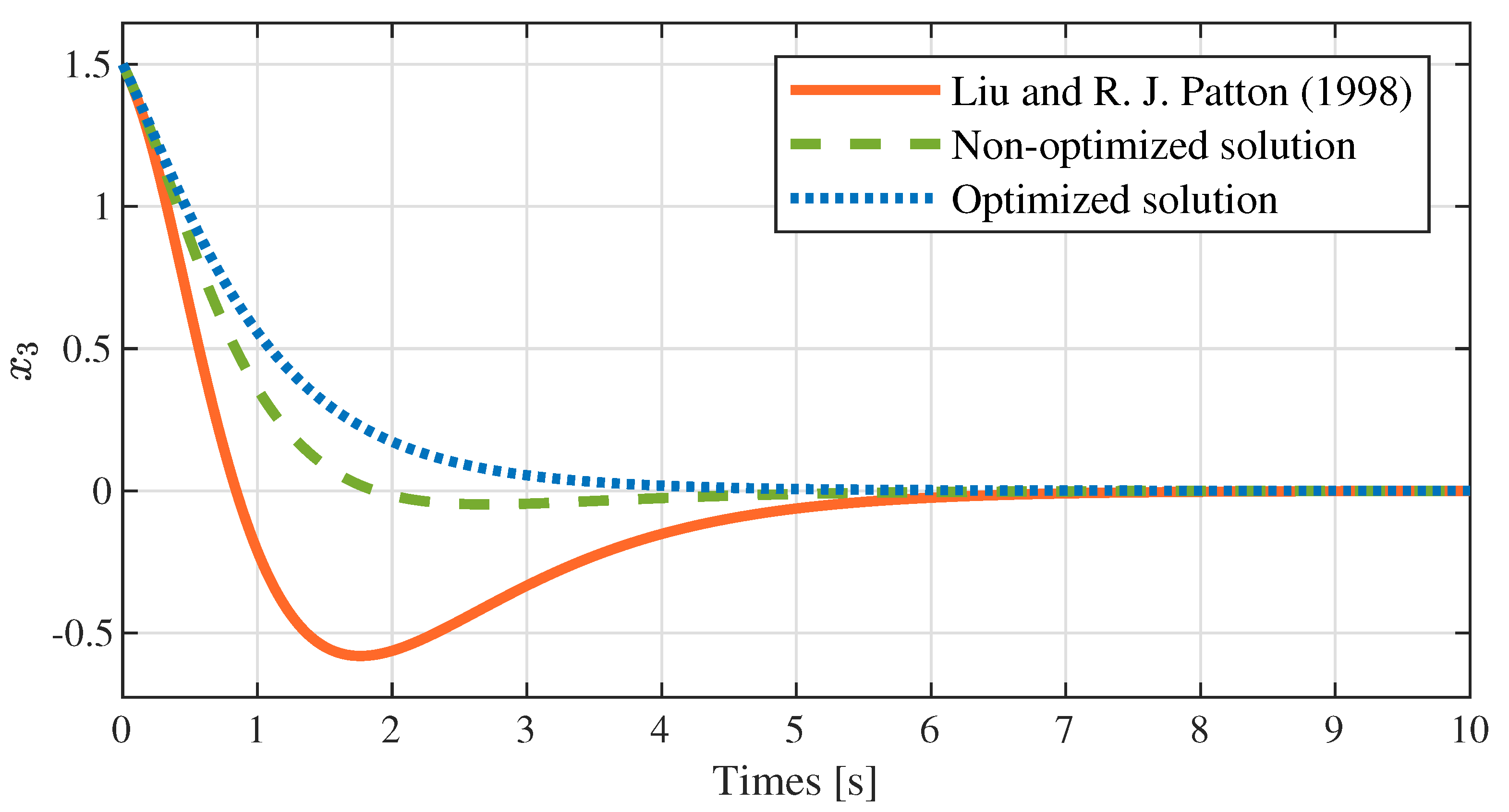
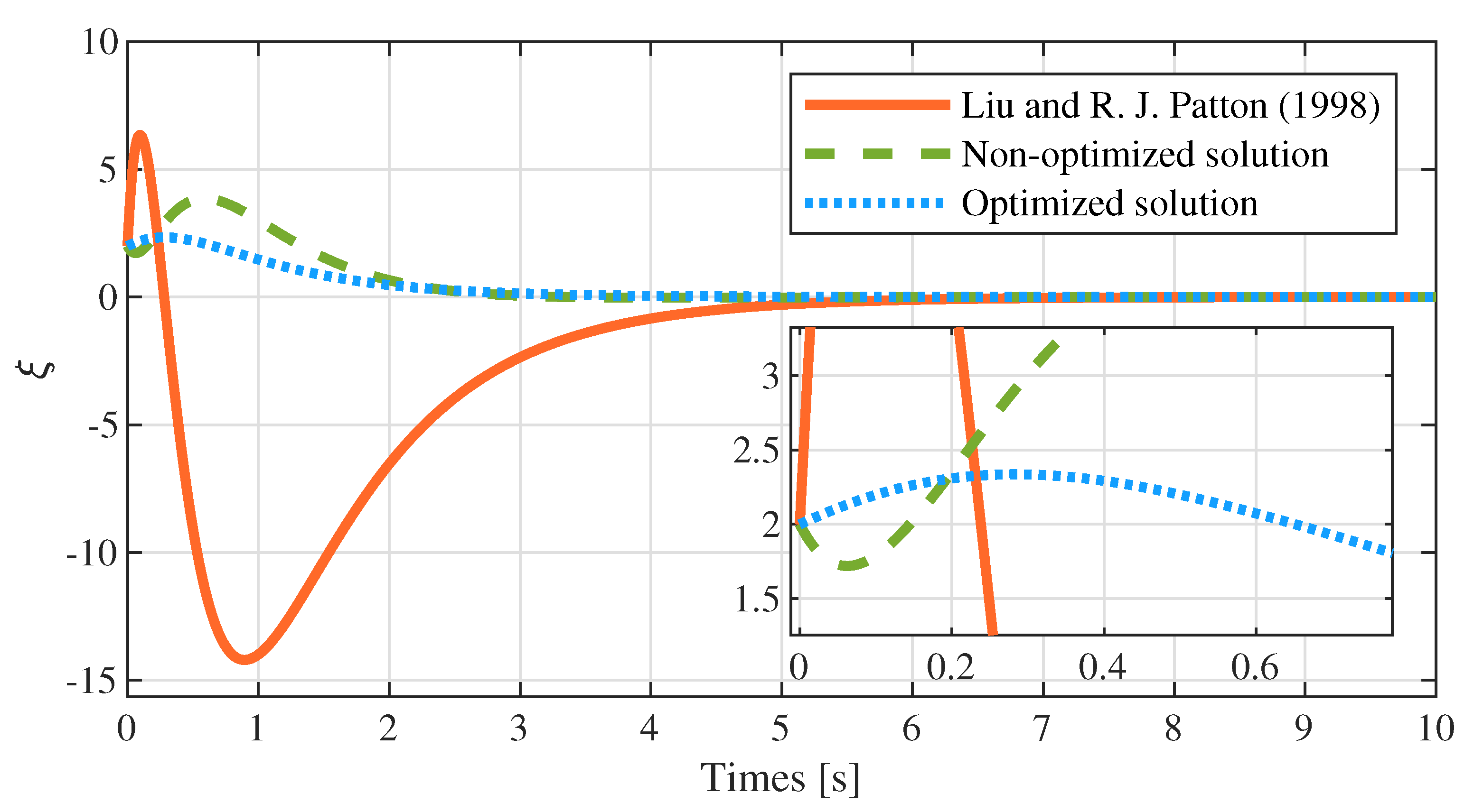
• It is not difficult to find from Figure 2, Figure 3 and Figure 4 that the state variables of the closed-loop system tend to zero in both the optimized and non-optimized solutions, which indicates that the closed-loop system is stable and that the parametric method proposed in this paper is effective.
• Compared with Liu et al. in [32], the method presented in this paper greatly enhances the overall performance of the system. Specifically, Table 2 shows that the precision of the closed-loop system’s eigenvalues is improved, and Table 3, Table 4 and

  Table 5. Comparison of the rapidity between three solutions.

  Error	Value(s)
  	${\mathit{x}}_{\mathbf{1}}<{\mathbf{10}}^{-\mathbf{3}}$	${\mathit{x}}_{\mathbf{2}}<{\mathbf{10}}^{-\mathbf{3}}$	${\mathit{x}}_{\mathbf{3}}<{\mathbf{10}}^{-\mathbf{3}}$	$\mathit{\xi }<{\mathbf{10}}^{-\mathbf{3}}$
  Liu et al. [32]	9.248	9.123	9.374	>10
  Non-optimized solution	7.560	7.438	7.683	8.500
  Optimized solution	6.693	6.699	6.693	7.534

  illustrate that the object function, maximum amplitude and expected error are greatly reduced, respectively.
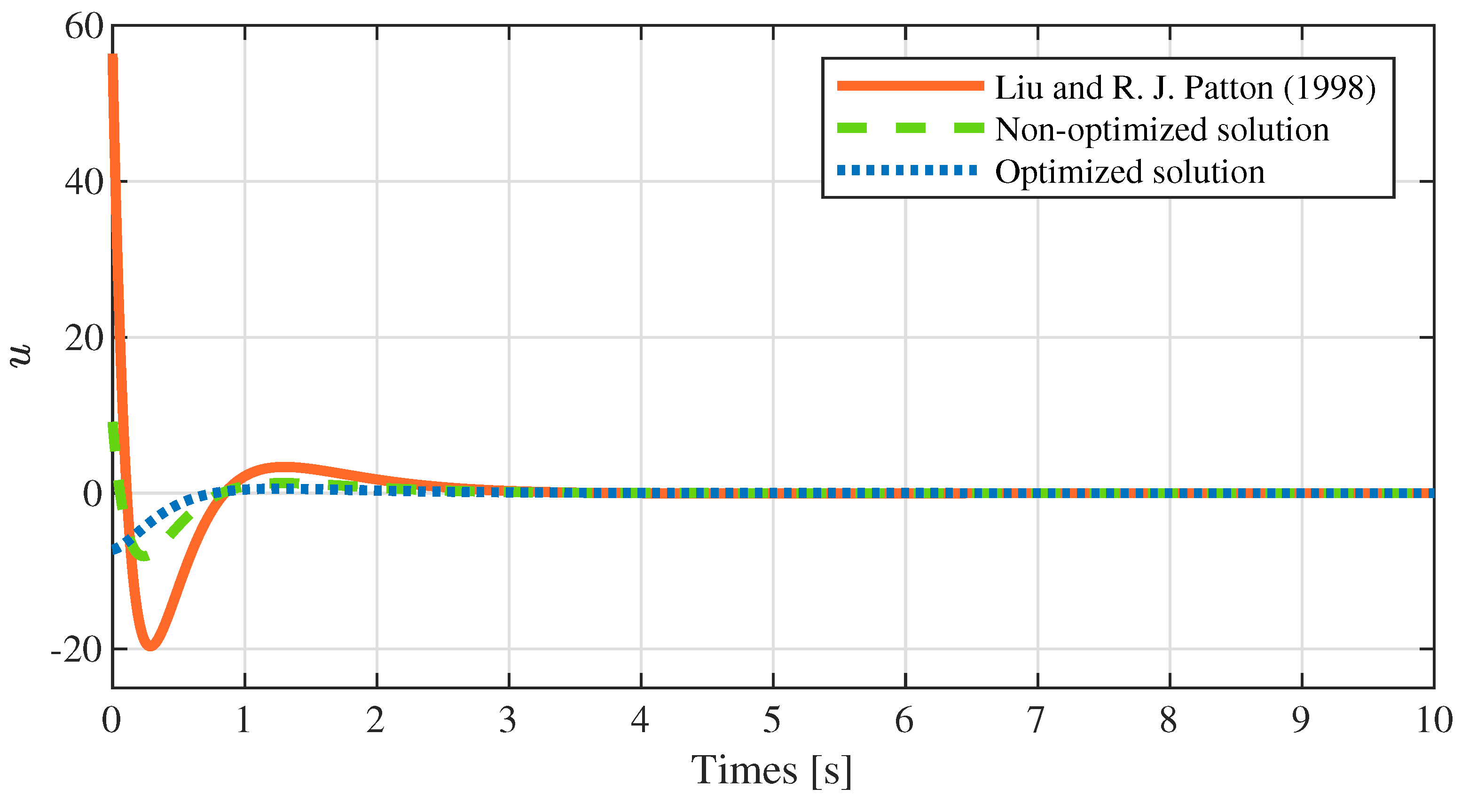
• The optimized dynamic compensator achieves superior control performance to Liu and the non-optimized dynamic compensator by utilizing the degrees of freedom offered in the parameter matrices (see Figure 5). Meanwhile, the optimized solution consumes less energy than the non-optimized solution and that of Liu (see control input in Figure 1).

Remark 4.

Through the data in the above simulation diagrams and tables, we can summarize two highlights of the method proposed in this paper. Firstly, we introduce a class of dynamic compensators and obtain the desired closed-loop eigenstructure, which makes up for the defect that the static output feedback cannot arbitrarily assign poles. Secondly, the degrees of freedom provided by two groups of arbitrary parameter matrices $Z_l$ and $Z_r$ in the parameter solution are directly utilized to realize the additional system design requirements.

Remark 5.

For the classical solutions to the problem PEA, the design process in [33,34] involves too many matrices calculation, so their results are complicated and without degrees of freedom. However, the greatest strength of the parametric method is that it can provide all degrees of freedom of design. In this paper, it is represented by two groups of arbitrary parameters $Z_l$ and $Z_r$. The selection of parameters only needs to meet several simple constraints, so it is very feasible. The eigenvalues of the closed-loop system ${\lambda }_l,{\lambda }_i^r,i=1,2,3$ in (69) may even be set undetermined and used as a part of the degrees of freedom as well. This possibility will be taken into account in more detail in subsequent work.

8. Conclusions

In this paper, a dynamic compensator-based parametric design approach for a class of linear systems is proposed. Based on the solutions of GSE, we only need to assign a subset of the left and right eigenvectors to obtain the desired closed-loop system eigenstructure, which reduces a large number of complex constraints, so the design of the controller will become simpler and cost effective. At the same time, the parametric expression of the dynamic output feedback controller is established based on two groups of parameter matrices $Z_r$ and $Z_l$, which realize the arbitrary pole assignment of the closed-loop system. Finally, an example and the simulation results are given, which further demonstrate the proposed approach’s effectiveness. More importantly, the degrees of freedom in $Z_r$ and $Z_l$ may be completely utilized to meet the additional design needs of the system, which is the main advantage of our proposed method.

References

- Duan, G.R.; Liu, G.P. Complete parametric approach for eigenstructure assignment in a class of second-order linear systems. Automatica 2002, 38, 725–729. [Google Scholar] [CrossRef]
- Rastgaar, M.; Ahmadian, M.; Southward, S. A review on eigenstructure assignment methods and orthogonal eigenstructure control of structural vibrations. Shock Vib. 2009, 16, 555–564. [Google Scholar] [CrossRef]
- Wang, G.S.; Liang, B.; Lv, Q.; Duan, G.R. Eigenstructure Assignment in Second-order Linear Systems: A Parametric Design Method. In Proceedings of the 2007 Chinese Control Conference, Zhangjiajie, China, 26–31 July 2007; pp. 9–13. [Google Scholar] [CrossRef]
- Gu, D.K.; Zhao, D.J.; Liu, Y.D.; Fu, Y.M. Complete parametric approach for eigenstructure assignment in second-order systems using displacement-plus-acceleration feedback. In Proceedings of the 2016 22nd International Conference on Automation and Computing (ICAC), Colchester, UK, 7–8 September 2016; pp. 183–187. [Google Scholar] [CrossRef]
- White, B. Eigenstructure assignment: A survey. Proc. Inst. Mech. Eng. P. J. Syst. Control 1995, 209, 1–11. [Google Scholar] [CrossRef]
- Lee, T.H. Adjoint method for design sensitivity analysis of multiple eigenvalues and associated eigenvectors. AIAA J. 2007, 45, 1998–2004. [Google Scholar] [CrossRef]
- Zhou, T.; Zhu, C. Robust Proportional-Differential Control via Eigenstructure Assignment for Active Magnetic Bearings-Rigid Rotor Systems. IEEE. Trans Ind. Electron. 2022, 69, 6572–6585. [Google Scholar] [CrossRef]
- Pal, M.; Bera, T. A Probabilistically Robust Eigenstructure Assignment Technique for Flight Control Design of UAVs. In Proceedings of the 2021 IEEE Aerospace Conference (50100), Big Sky, MT, USA, 6–13 March 2021; pp. 1–11. [Google Scholar] [CrossRef]
- Gu, D.K.; Zhang, D.W. Parametric control to a type of descriptor quasi-linear high-order systems via output feedback. Eur. J. Control 2021, 58, 223–231. [Google Scholar] [CrossRef]
- Baddou, A.; Maarouf, H.; Benzaouia, A. Partial eigenstructure assignment problem and its application to the constrained linear problem. Int. J. Syst. Sci. 2013, 44, 908–915. [Google Scholar] [CrossRef]
- Duan, G.R.; Irwin, G.W.; Liu, G.P. Partial eigenstructure assignment by state feedback: A complete parametric approach. In Proceedings of the 1999 European Control Conference (ECC), Karlsruhe, Germany, 31 August–3 September 1999; pp. 1890–1895. [Google Scholar] [CrossRef]
- Duan, G.R.; Wang, G.S. Partial eigenstructure assignment for descriptor linear systems: A complete parametric approach. In Proceedings of the 42nd IEEE International Conference on Decision and Control (IEEE Cat. No. 03CH37475), Maui, HI, USA, 9–12 December 2003; Volume 4, pp. 3402–3407. [Google Scholar] [CrossRef]
- Duan, G.R. Circulation algorithm for partial eigenstructure assignment via state feedback. Eur. J. Control 2019, 50, 107–116. [Google Scholar] [CrossRef]
- Gu, D.K.; Wang, R.Y.; Liu, Y.D. A parametric approach of partial eigenstructure assignment for high-order linear systems via proportional plus derivative state feedback. AIMS Math. 2021, 6, 11139–11166. [Google Scholar] [CrossRef]
- Gu, D.K.; Duan, S.; Wang, R.Y.; Liu, Y.D. Parametric design method for partial eigenstructure assignment of second-order linear systems via observer-based state feedback. Eur. J. Control 2023, 71, 100801. [Google Scholar] [CrossRef]
- Gu, D.K.; Wang, R.Y.; Liu, Y.D. Partial eigenstructure assignment for descriptor high-order linear systems via proportional plus derivative state feedback: A parametric approach. Trans. Inst. Meas. Control 2023, 01423312221150295. [Google Scholar] [CrossRef]
- Zhang, J.; Ouyang, H.; Yang, J. Partial eigenstructure assignment for undamped vibration systems using acceleration and displacement feedback. J. Sound. Vib. 2014, 333, 1–12. [Google Scholar] [CrossRef]
- Zhang, J.; Ouyang, H.; Zhang, Y.; Ye, J. Partial quadratic eigenvalue assignment in vibrating systems using acceleration and velocity feedback. Inverse. Probl. Sci. Eng. 2015, 23, 479–497. [Google Scholar] [CrossRef]
- Zhang, J.; Ye, J.; Ouyang, H. Static output feedback for partial eigenstructure assignment of undamped vibration systems. Mech. Syst. Signal. Process. 2016, 68, 555–561. [Google Scholar] [CrossRef]
- Belotti, R.; Richiedei, D.; Trevisani, A. Optimal design of vibrating systems through partial eigenstructure assignment. J. Mech. Des. 2016, 138, 071402. [Google Scholar] [CrossRef]
- Bai, Z.J.; Datta, B.N.; Wang, J. Robust and minimum norm partial quadratic eigenvalue assignment in vibrating systems: A new optimization approach. Mech. Syst. Signal. Process. 2010, 24, 766–783. [Google Scholar] [CrossRef] [Green Version]
- Zhang, L.; Yu, F.; Wang, X. An algorithm of partial eigenstructure assignment for high-order systems. Math. Methods. Appl. Sci. 2018, 41, 6070–6079. [Google Scholar] [CrossRef]
- Yu, P. Partial eigenstructure assignment problem for vibration system via feedback control. Asian. J. Control 2022, 24, 297–308. [Google Scholar] [CrossRef]
- Gu, D.K.; Zhang, D.W. Parametric control to second-order linear time-varying systems based on dynamic compensator and multi-objective optimization. Appl. Math. Comput. 2020, 365, 124681. [Google Scholar] [CrossRef]
- Gu, D.K.; Zhang, D.W. A parametric method to design dynamic compensator for high-order quasi-linear systems. Nonlinear Dyn. 2020, 100, 1379–1400. [Google Scholar] [CrossRef]
- Duan, G.R. On a type of generalized sylvester equations. In Proceedings of the 2013 25th Chinese Control and Decision Conference (CCDC), Guiyang, China, 25–27 May 2013; pp. 1264–1269. [Google Scholar] [CrossRef]
- Duan, G.R. Generalized Sylvester Equations: Unified Parametric Solutions; CRC Press: Boca Raton, FL, USA, 2015. [Google Scholar]
- dos Santos, J.F.S.; Pellanda, P.C.; Simoes, A.M. Robust pole placement under structural constraints. Syst. Control Lett. 2018, 116, 8–14. [Google Scholar] [CrossRef]
- Wang, X.T.; Zhang, L. Partial eigenvalue assignment with time delay in high order system using the receptance. Linear Algebra. Appl. 2017, 523, 335–345. [Google Scholar] [CrossRef]
- Duan, G.R. Parametric eigenstructure assignment via output feedback based on singular value decompositions. IEEE. Int. Conf. Control. Autom. 2003, 150, 93–100. [Google Scholar] [CrossRef]
- Zhang, B. Eigenstructure assignment for linear descriptor systems via output feedback. Asian. J. Control 2019, 21, 759–769. [Google Scholar] [CrossRef]
- Liu, G.P.; Patton, R. Eigenstructure Assignment for Control System Design; John Wiley & Sons, Inc.: Hoboken, NJ, USA, 1998. [Google Scholar]
- Lu, J.; Chiang, H.D.; Thorp, J.S. Partial eigenstructure assignment and its application to large scale systems. IEEE Trans. Automat. Control 1991, 36, 340–347. [Google Scholar] [CrossRef]
- Satoh, A.; Sugimoto, K. Partial eigenstructure assignment approach for robust flight control. J. Guid. Control Dyn. 2004, 27, 145–150. [Google Scholar] [CrossRef]
Figure 1.
Variation diagram of control input u.
Figure 2.
Variation diagram of state variable .
Figure 3.
Figure 4.
Figure 5.
Variation diagram of compensation vector .