Spectral Analysis of the Infinite-Dimensional Sonic Drillstring Dynamics

Abstract

By deploying sonic drilling for soil structure fracturing in the presence of consolidated/ unconsolidated formations, this technique greatly reduces the friction on the drillstring and bit by using energetic resonance, a bit-bouncing high-frequency axial vibration. While resonance must be avoided, to our knowledge, drilling is the only application area where resonance is necessary to break up the rocks. The problem is that the machine’s tool can encounter several different geological layers with many varieties of density. Hence, keeping the resonance of the tool plays an important role in drill processes, especially in tunnel or infrastructure shoring. In this paper, we analyze the sonic drillstring dynamics as an infinite-dimensional system from another viewpoint using the frequency domain approach. From the operator theory in defining the adequate function spaces, we show the system well-posedness. The hydraulic produced axial force that should preserve the resonant drillstring mode is defined from the spectrum study of the constructed linear operator guided by the ratio control from the top to tip boundary magnitudes.

1. Introduction

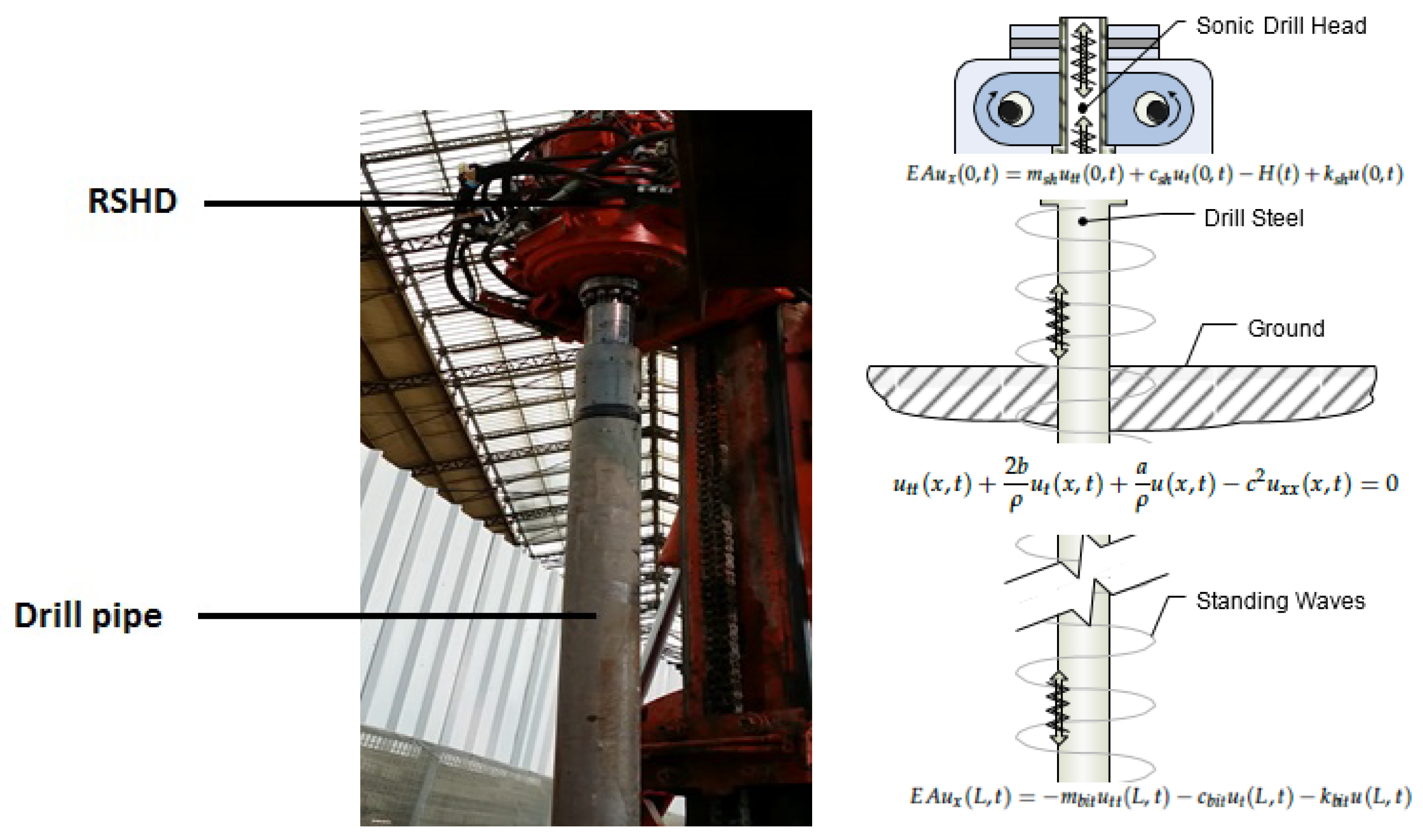
Sonic drilling has been used in industry for many years [1,2,3,4]. This technique makes penetrating for a large range of soils much easier. Most of the research has been conducted by the private sector, which has kept the expertise it has developed in-house and proprietary [5]. However, it is known from the current field studies that the main source of drillstring vibration is the force generated by two eccentric masses coupled to a hydraulic system. It can be defined as a harmonic force for deriving the mathematical equations. In reality, the excited force depends on the rock mechanical properties, the shape of the drill bit, the frequency of the masses, the air pressure, and the cross-sectional area of the hammer. In [6], bond graph modeling formalism is used to develop drillstring dynamics. Currently, sonic drilling rigs are operated mainly by “feel” and “ear.” Although equipped with numerous gages, the success of sonic drilling depends on the experience of the operator; less experienced drillers are not successful on sonic rigs. The main objective is to keep the drillstring resonant [7,8]. Technically, resonant frequencies of 50 to 150 Hz are audible, and the driller controls the energy generated by the sonic eccentrics according to the formation encountered to achieve maximum drilling productivity. If the damper cannot absorb all the energy entering the system, the vibration amplitude of the system will increase until the system fails. Therefore, the input force is an important operating parameter and a primary point of tuning to produce the maximum amplitude when the frequency of the vibration matches the natural frequency of vibration of the system (resonant frequency). Once the frequency is set, the operator manually moves the column and verifies that the tool moves smoothly while ensuring that the vibration mode is maintained during the penetration of the soil (see Figure 1). This process takes a lot of time and can have a negative impact on operating costs and machine loss. In the Newtun project, proposed as an alternative to conventional tunnel excavation [9], the reader will learn more details about the experimental drilling method: the type of drilling rig used, type of rock, type of drill pipe, drilling tools, etc.

Drillstring dynamics modeling is critical for the system analysis and control of damaging vibrations. Much research has been conducted to mathematically describe the physical phenomena that occur during the drilling process. Starting from linear algebra theory, researchers began with models with lumped parameters in which the drillstring is viewed as a mass-spring-damper system whose dynamics are described by an ordinary differential equation (ODE) (see [10,11,12,13,14]). This finite-dimensional system representation did not respect the distributed nature of the drilling structure. Consequently, distributed parameter models appeared and they provided a characterization of the drilling variables in an infinite dimension which added more accuracy to the model in reproducing the rod oscillatory behavior. For the case of a distributed parameter model, see [15,16,17,18,19,20,21]. The drawback of this second type of modeling was the complexity involved in its analysis and simulations. Then arose the neutral-type time-delay models which were directly derived from the distributed parameter ones. The transformation of the partial differential equations (PDE) model to the time-delay system was first introduced in [22]. This kind of modeling was used in [23,24,25,26,27] for control purposes.

This paper is organized as follows. In Section 2, we derive the mathematical model that describes the sonic drillstring dynamics. The drillstring dynamic global existence and the uniqueness of the solution is detailed in Section 3 (well-posedness). In Section 4, we analyze the spectrum of the defined operator and its exponential stability, and we prove that the operator does not contain a point on the imaginary axis. The details of the spectral analysis and the numerical results are presented in Section 5. Finally, some conclusions are part of Section 6.

Figure 1. Resonant sonic drill machinery for tunnel consolidation in Paris La Defense [28]. The right picture provided courtesy of Resodyn Corporation [7]. Annotations follow our mathematical analysis and the physical system parameters are given in

Table 1. Drillstring System Parameters [9].

L	76.2 m	ρ	7850 Kg/m3
E	2.1 × 10${}^{11}$ Pa	A	8.6 × 10${}^{-3}$ m${}^2$
$m_{sh}$	453.6 Kg	$m_{bit}$	8 Kg
$k_{sh}$	84,040,034.023 N/m	$c_{sh}$	10 N.S/m
$c^2=E/rho$	2.6752 × 10${}^7$ m${}^2/$s${}^2$	$m_{ec}$	28.4 Kg
$r_{ec}$	0.06 m	$k_{bit}$	1194.519 N/m
$c_{bit}$	0 N.s/m	b	0 N.s/m${}^4$
a	2334.434 N/m${}^4$	$\zeta$	50–200 Hz

.

Figure 1. Resonant sonic drill machinery for tunnel consolidation in Paris La Defense [28]. The right picture provided courtesy of Resodyn Corporation [7]. Annotations follow our mathematical analysis and the physical system parameters are given in Table 1.

2. Mathematical Model

In order to reduce the complexity of the system and thus derive a mathematical model, it is necessary to make some initial assumptions and simplifications of the system when choosing the boundary conditions [29]. It is assumed that the drillstring is a long pipe with a uniform cross-sectional area A and the effect of torsional vibrations is negligible. It is assumed that the forces exciting the drillstring act at the tip of the sonic drill. Because the damping along the length is very small, the sonic drill operator must be very careful not to overload the drillstring at resonance when the lower drill tip is not involved in drilling. Damping at the drill tip is the most important variable of the drilling system because it determines the drilling work that takes place.

The governing differential equations of motion for the sonic drill are derived from the force balance. We denote by $u\left(x,t\right)$ the longitudinal displacement of a rod’s section A, that is, a distance x from the vertices at time t.

$$\begin{array}{c}\hfill \rho Adx{u}_{tt}\left(x,t\right)+2bAdx{u}_t\left(x,t\right)+aAdxu\left(x,t\right)\\ \hfill +\sigma A-\left(\sigma .A+{\left(\sigma .A\right)}_{x}dx\right)=0\end{array}$$

(1)

where $\rho$ is the pipe density, E is the Young modulus, a and b are, respectively, the coupling and damping constants along the length of the drillstring, and $\sigma$ is the stress given by $\sigma =E{u}_x\left(x,t\right)$. So, we obtain

$$\begin{array}{c}\hfill \rho Adx{u}_{tt}\left(x,t\right)+2bAdx{u}_t\left(x,t\right)+aAdxu\left(x,t\right)\\ \hfill -EAdx{u}_{xx}\left(x,t\right)=0\end{array}$$

(2)

Dividing this last by $\rho Adx$, we obtain

$$u_{tt}\left(x,t\right)+\frac{2b}{\rho }{u}_t\left(x,t\right)+\frac{a}{\rho }u\left(x,t\right)-\frac{E}{\rho }{u}_{xx}\left(x,t\right)=0$$

(3)

We define the speed of the sound through the steel drill c by $c=\sqrt{\frac{E}{\rho }}$.

Equation (3) becomes

$$\begin{array}{c}\hfill u_{tt}\left(x,t\right)+\frac{2b}{\rho }{u}_t\left(x,t\right)+\frac{a}{\rho }u\left(x,t\right)-c^2{u}_{xx}\left(x,t\right)=0\end{array}$$

(4)

With $(x,t)\in (0,L)\times {\mathbb{R}}_{+}$. It remains to define the boundary conditions of the drillstring dynamics given above.

To calculate the natural frequencies of the drillstring, the boundary conditions at the ends of the string must be known when deriving the frequency functions. The mass of the sonic driver, the input force of the sonic driver, and the air spring are all located where x is zero. The mass of the sonic driver and the air spring are always boundary conditions. At the drillstring tip, where x equals the drillstring length L, there is a boundary condition caused by the coupling of the sonic drill tip to the material being drilled through. All boundary conditions are at the ends of the drillstring, and therefore all conditions must equal the apparent forces at the end conditions. The forces for the ends are determined by multiplying the elastic constant E of the drillstring by the cross-sectional area of the drillstring A, and also by the partial derivative of the local deflection u with respect to the location in space x, and equating this to the boundary condition, as shown in Figure 1 (right).

Top boundary condition ($t>0$):

$$EA{u}_x\left(0,t\right)=m_{sh}{u}_{tt}\left(0,t\right)+c_{sh}{u}_t\left(0,t\right)-H\left(t\right)+k_{sh}u\left(0,t\right)$$

(5)

where $m_{sh}$ is the mass of the sonic head, $k_{sh}$ and $c_{sh}$ are, respectively, the spring and the damping rates of the air spring on top of the sonic drill.

Tip boundary condition ($t>0$):

$$EA{u}_x\left(L,t\right)=-m_{bit}{u}_{tt}\left(L,t\right)-c_{bit}{u}_t\left(L,t\right)-k_{bit}u\left(L,t\right)$$

(6)

and the initial conditions are

$$u(x,0)=0,u_t(x,0)=0,x\in (0,L),$$

(7)

where $m_{bit}$ is the mass of the sonic drill bit, $k_{bit}$ and $c_{bit}$ are, respectively, the spring and the damping rates of the drill bit while drilling.

3. Well-Posedness

In this section, we will prove the global existence and the uniqueness of the solution of the problem (3)–(7). For this purpose, we will use a semigroup formulation of the initial-boundary value problem (3)–(7). If we denote $V:={\left(u,u_t,u\left(0\right),u_t\left(0\right),u\left(L\right),u_t\left(L\right)\right)}^T$, we define the energy space:

$$\begin{array}{c}\hfill \mathcal{H}=\{(u,v,w_1,w_2,z_1,z_2)\in H^1(0,L)\times L^2(0,L)\times {\mathbb{R}}^4,w_1=u\left(0\right),z_1=u\left(L\right)\}\end{array}$$

(8)

Clearly, $\mathcal{H}$ is a Hilbert space with respect to the inner product

$$\begin{array}{c}\hfill {〈V_1,V_2〉}_{\mathcal{H}}=\frac{a}{\rho }{\int }_0^L{u}^1{u}^{2}dx+c^2{\int }_0^L{u}_x^1{u}_x^{2}dx+{\int }_0^L{v}^1{v}^{2}dx\\ \hfill +c^2\frac{k_{sh}}{EA}{a}_1{b}_1+c^2\frac{m_{sh}}{EA}{a}_2{b}_2+c^2\frac{k_{bit}}{EA}{c}_1{d}_1+c^2\frac{m_{bit}}{EA}{c}_2{d}_2\end{array}$$

(9)

for

$V_1={(u^1,v^1,a_1,a_2,c_1,c_2)}^T$, $V_2={(u^2,v^2,b_1,b_2,d_1,d_2)}^T.$

Therefore if $H\in L^2(0,+\infty )$, the problem (3)–(7) is formally equivalent to the following abstract evolution equation in the Hilbert space $\mathcal{H}$:

$$\left\{\begin{array}{c}{V}^{\prime }\left(t\right)=\mathcal{A}V\left(t\right)+\mathcal{B}H\left(t\right),t>0,\hfill \\ V\left(0\right)=0\hfill \end{array}\right.$$

(10)

where ${}^{\prime }$ denotes the derivative with respect to time t.

The operator $\mathcal{A}$ is defined by

$$\mathcal{A}\left(\begin{array}{c}u\\ v\\ w_1\\ w_2\\ z_1\\ z_2\end{array}\right)=\left(\begin{array}{c}{\displaystyle v}\\ {\displaystyle c^2{u}_{xx}-\frac{2b}{\rho }v-\frac{a}{\rho }u}\\ w_2\\ {\displaystyle \frac{EA}{m_{sh}}{u}_x\left(0\right)-\frac{c_{sh}}{m_{sh}}{w}_2-\frac{k_{sh}}{m_{sh}}{w}_1}\\ z_2\\ {\displaystyle -\frac{EA}{m_{bit}}{u}_x\left(L\right)-\frac{c_{bit}}{m_{bit}}{z}_2-\frac{k_{bit}}{m_{bit}}{z}_1}\end{array}\right)\mathrm{and}\mathcal{B}:=\left(\begin{array}{c}0\hfill \\ 0\hfill \\ 0\hfill \\ \frac{1}{m_{sh}}\hfill \\ 0\hfill \\ 0\hfill \end{array}\right)$$

(11)

The domain of $\mathcal{A}$ is given by

$$\begin{array}{c}\hfill \mathcal{D}\left(\mathcal{A}\right)=\{{(u,v,w_1,w_2,z_1,z_2)}^T\in \mathcal{H};u\in H^2(0,L),v\in H^1(0,L),w_2=v\left(0\right),z_2=v\left(L\right)\}\end{array}$$

We have the following.

Theorem 1. 

The operator $\mathcal{A}$ generates a $C_0$ semigroup of contractions ${\left(e^{t\mathcal{A}}\right)}_{t\ge 0}$ on $\mathcal{H}$.

Proof. 

According to the Lumer–Phillips theorem, we should prove that the operator $\mathcal{A}$ is m-dissipative.

Let $V={(u,v,w_1,w_2,z_1,z_2)}^T\in \mathcal{D}\left(\mathcal{A}\right)$. By definition of the operator $\mathcal{A}$ and the scalar product of $\mathcal{H}$, we have

$${〈\mathcal{A}V,V〉}_{\mathcal{H}}=\frac{a}{\rho }{\int }_0^{L}v\left(x\right)u\left(x\right)dx+c^2{\int }_0^L{v}_x\left(x\right)u_x\left(x\right)dx+$$

$${\int }_0^L\left(c^2{u}_{xx}\left(x\right)-\frac{2b}{\rho }v\left(x\right)-\frac{a}{\rho }\right)v\left(x\right)dx+c^2\frac{k_{sh}}{EA}{w}_2{w}_1+$$

$$c^2\frac{m_{sh}}{EA}\left(\frac{EA}{m_{sh}}{u}_x\left(0\right)-\frac{c_{sh}}{m_{sh}}{w}_2-\frac{k_{sh}}{m_{sh}}{w}_1\right)w_2+c^2\frac{k_{bit}}{EA}{z}_1{z}_2+$$

$$c^2\frac{m_{bit}}{EA}\left(-\frac{EA}{m_{bit}}{u}_x\left(L\right)-\frac{c_{bit}}{m_{bit}}{z}_2-\frac{k_{bit}}{m_{bit}}{z}_1\right)z_2$$

From Green’s formula, we obtain

$${〈\mathcal{A}V,V〉}_{\mathcal{H}}=-\frac{2b}{\rho }{\int }_0^L{v}^2\left(x\right)dx-c^2\frac{c_{sh}}{EA}{w}_2^2-c^2\frac{k_{bit}}{EA}{z}_2^2\le 0.$$

(12)

Consequently the operator $\mathcal{A}$ is dissipative.

Now, we want to show that for $\lambda >0,\lambda I-\mathcal{A}$ is surjective.

For $F={(f_1,f_2,f_3,f_4,f_5,f_6)}^T\in \mathcal{H}$, let $V={(u,v,w_1,w_2,z_1,z_2)}^T\in \mathcal{D}\left(\mathcal{A}\right)$ be the solution of

$$\left(\lambda I-\mathcal{A}\right)V=F$$

(13)

which leads to

$$\begin{array}{cc}\hfill \lambda u-v& =f_1,\end{array}$$

(14)

$$\begin{array}{cc}\hfill \lambda v-c^2{u}_{xx}+\frac{2b}{\rho }v+\frac{a}{\rho }u& =f_2,\end{array}$$

(15)

$$\begin{array}{cc}\hfill \lambda w_1-w_2& =f_3,\end{array}$$

(16)

$$\begin{array}{cc}\hfill \lambda w_2-\frac{EA}{m_{sh}}{u}_x\left(0\right)+\frac{c_{sh}}{m_{sh}}{w}_2+\frac{k_{sh}}{m_{sh}}{w}_1& =f_4\end{array}$$

(17)

$$\begin{array}{cc}\hfill \lambda z_1-z_2& =f_5\end{array}$$

(18)

$$\begin{array}{cc}\hfill \lambda z_2+\frac{EA}{m_{bit}}{u}_x\left(L\right)+\frac{c_{bit}}{m_{bit}}{z}_2+\frac{k_{bit}}{m_{bit}}{z}_1& =f_6.\end{array}$$

(19)

To find the $V={(u,v,w_1,w_2,z_1,z_2)}^T\in \mathcal{D}\left(\mathcal{A}\right)$ solution of the system (14)–(19), we suppose u is determined with the appropriate regularity. Then, from (14), (16), and (18), we obtain

$$v=\lambda u-f_1,w_2=\lambda u\left(0\right)-f_3,z_2=\lambda u\left(L\right)-f_5.$$

(20)

Consequently, knowing u, we may deduce $v,w_1=u\left(0\right),w_2,z_1=u\left(L\right),z_2$ by (20).

We recall that because $V={(u,v,w_1,w_2,z_1,z_2)}^T\in \mathcal{D}\left(\mathcal{A}\right)$, we automatically obtain $w_2=v\left(0\right)$ and $z_2=v\left(L\right)$.

From Equations (15), (17), (19), and (20), u must satisfy

$${\lambda }^{2}u-c^2{u}_{xx}+\frac{2b}{\rho }\lambda u+\frac{a}{\rho }u=f_2+\frac{2b}{\rho }{f}_1+\lambda f_1,in(0,L)$$

(21)

with the boundary conditions

$$\begin{array}{cc}\hfill {\lambda }^{2}u\left(0\right)-\frac{EA}{m_{sh}}{u}_x\left(0\right)+\lambda \frac{c_{sh}}{m_{sh}}u\left(0\right)+\frac{k_{sh}}{m_{sh}}u\left(0\right)=f_4+\lambda f_3+\frac{c_{sh}}{m_{sh}}{f}_3,& \end{array}$$

(22)

$$\begin{array}{c}\hfill {\lambda }^{2}u\left(L\right)+\frac{EA}{m_{bit}}{u}_x\left(L\right)+\lambda \frac{c_{bit}}{m_{bit}}u\left(L\right)+\frac{k_{bit}}{m_{bit}}u\left(L\right)=f_6+\lambda f_5+\frac{c_{bit}}{m_{bit}}{f}_5.\end{array}$$

(23)

The variational formulation of problem (21), (22) is to find $(u,w_1,z_1)\in H:=\left\{(u,w_1,z_1);\omega \in H^1(0,L),w_1=u\left(0\right),z_1=u\left(L\right)\right\}$ such that

$$\begin{array}{c}\hfill {\int }_0^L\left\{\left({\lambda }^2+\frac{2b}{\rho }\lambda +\frac{a}{\rho }\right)u\omega +u_x{\omega }_x\right\}dx+c^2\frac{m_{sh}}{EA}\left({\lambda }^2+\lambda \frac{c_{sh}}{m_{sh}}+\frac{k_{sh}}{m_{sh}}\right)u\left(0\right)w\left(0\right)\\ \hfill +c^2\frac{m_{bit}}{EA}\left({\lambda }^2+\lambda \frac{c_{bit}}{m_{bit}}+\frac{k_{bit}}{m_{bit}}\right)u\left(L\right)w\left(L\right)\\ \hfill ={\int }_0^L\left(f_2+\left(\lambda +\frac{2b}{\rho }\right)f_1\right)\omega dx+c^{2}w\left(0\right)\left(f_4+\lambda f_3+\frac{c_{sh}}{m_{sh}}{f}_3\right)\\ \hfill +c^{2}w\left(L\right)\left(f_6+\left(\lambda +\frac{c_{bit}}{m_{bit}}\right)f_5\right)\end{array}$$

(24)

for any $(\omega ,{\xi }_1,{\xi }_2)\in H$. Because $\lambda >0$, the left-hand side of (24) defines a coercive bilinear form on H. Thus, by applying the Lax–Milgram theorem, there exists a unique $(u,w_1,z_1)\in H$ solution of (24). Now, choosing $\omega \in {\mathcal{C}}_c^{\infty }$, $(u,w_1,z_1)$ is a solution of (21) in the sense of distribution and therefore $u\in H^2(0,L)$. Thus, using Green’s formula and exploiting Equation (21) on $(0,L)$, we finally obtain

$$\begin{array}{c}\hfill c^2\frac{m_{sh}}{EA}\left({\lambda }^2+\lambda \frac{c_{sh}}{m_{sh}}+\frac{k_{sh}}{m_{sh}}\right)w\left(0\right)u\left(0\right)+c^2\frac{m_{bit}}{EA}\left({\lambda }^2+\lambda \frac{c_{bit}}{m_{bit}}+\frac{k_{bit}}{m_{bit}}\right)w\left(L\right)u\left(L\right)\\ \hfill =c^2\frac{m_{sh}}{EA}\left(f_4+\left(\lambda +\frac{c_{sh}}{m_{sh}}\right)f_3\right)w\left(0\right)+c^2\frac{m_{bit}}{EA}\left(f_6+\left(\lambda +\frac{c_{bit}}{m_{bit}}\right)f_5\right)w\left(L\right)\end{array}$$

(25)

Thus $u\in H^2(0,L)$ verifies (17), (19) and we recover $u,w_1=u\left(0\right),z_1=u\left(L\right)$, and $v\in H^1(0,L)$, and thus by (20), we obtain $w_2=v\left(0\right),z_2=v\left(L\right),$ and we have found the $V={(u,v,w_1,w_2,z_1,z_2)}^T\in \mathcal{D}\left(\mathcal{A}\right)$ solution of $\left(I-\mathcal{A}\right)V=F$. This completes the proof of Theorem 1. □

We have, in particular, that the Cauchy abstract problem

$$\left\{\begin{array}{c}{Z}^{\prime }\left(t\right)=\mathcal{A}Z\left(t\right),t>0,\hfill \\ Z\left(0\right)=Z^0={(u^0,v^0,w_1^0,w_2^0,z_1^0,z_2^0)}^T\hfill \end{array}\right.$$

(26)

admits for all $Z^0\in \mathcal{H}$ a unique solution $Z\left(t\right)=e^{t\mathcal{A}}{Z}^0\in C\left({\mathbb{R}}_{+};\mathcal{H}\right)$. Moreover, for $Z^0\in \mathcal{D}\left(\mathcal{A}\right),$ the system (26) admits a unique solution

$$Z\left(t\right)=(u\left(t\right),u_t\left(t\right),u\left(0\right),u_t\left(0\right),u\left(L\right),u_t\left(L\right))\in C\left({\mathbb{R}}_{+};\mathcal{D}\left(\mathcal{A}\right)\right)$$

and satisfies the following energy identity:

$$\begin{array}{c}\hfill E\left(t\right)-E\left(0\right)=-\frac{2b}{\rho }{\int }_0^L{u}_t^2\left(x\right)dx-c^2\frac{c_{sh}}{EA}{u}_t^2(0,t)-c^2\frac{k_{bit}}{EA}{u}_t^2(L,t),\forall t\ge 0,\end{array}$$

(27)

where

$$E\left(t\right):=\frac{1}{2}{∥Z\left(t\right)∥}_{\mathcal{H}}^2,\forall t\ge 0.$$

(28)

Thus, the well-posedness of problem (3)–(7) is ensured by

Proposition 1. 

Let $H\in L^2(0,+\infty )$, and then there exists a unique solution

$$V\left(t\right)={\int }_0^t{e}^{(t-s)\mathcal{A}}\mathcal{B}H\left(s\right)ds\in C\left({\mathbb{R}}_{+};\mathcal{H}\right)$$

of problem (10).

4. Stability of the Semigroup ${\mathit{e}}^{\mathit{t}\mathcal{A}}$

Recall the following frequency domain theorem for exponential stability from [30,31] of a $C_0$-semigroup of contractions on a Hilbert space:

Theorem 2. 

Let A be the generator of a $C_0$-semigroup of contractions $S\left(t\right)$ on a Hilbert space X. Then, $e^{tA}$ is exponentially stable, i.e., for all $t>0$,

$$\left|\right|e^{tA}{\left|\right|}_{\mathcal{L}\left(X\right)}\le C{e}^{-\delta t},$$

for some positive constants C and δ if and only if

$$\rho \left(A\right)\supset \left\{i\gamma \right|\gamma \in \mathbb{R}\}\equiv i\mathbb{R},$$

(29)

and

$$\underset{\left|\gamma \right|\to +\infty }{lim\; sup}\parallel (i\gamma I-A^{-1}{\parallel }_{\mathcal{L}\left(X\right)}<\infty ,$$

(30)

where $\rho \left(A\right)$ denotes the resolvent set of the operator A.

We are now in a position to state the first main result of this section:

Theorem 3. 

There exists $C,\delta >0$ such that

$${∥e^{t\mathcal{A}}∥}_{\mathcal{L}\left(\mathcal{H}\right)}\le C{e}^{-\delta t},\forall t>0.$$

Proof. 

Our first concern is to show that $i\gamma$ is not on the spectra of $\mathcal{A}$ for any real number $\gamma$, which clearly implies (29). We have the following:

Lemma 1. 

The spectrum of $\mathcal{A}$ contains no point on the imaginary axis.

Proof. 

Because the resolvent of $\mathcal{A}$ is compact, its spectrum $\sigma \left(\mathcal{A}\right)$ only consists of eigenvalues of $\mathcal{A}$. We will show that the equation

$$\mathcal{A}V=i\beta V$$

(31)

with $V={(u,v,w_1,w_2,z_1,z_2)}^T\in \mathcal{D}\left(A\right)$ and $\beta \in \mathbb{R}$ has only the trivial solution.

By taking the inner product of (31) with V and using

$$\Re {\langle \mathcal{A}V,V\rangle }_{\mathcal{H}}=-\frac{2b}{\rho }{\int }_0^L{v}^2\left(x\right)dx-c^2\frac{c_{sh}}{EA}{w}_2^2-c^2\frac{k_{bit}}{EA}{z}_2^2$$

(32)

one obtains $v=0,w_2=0,z_2=0$. Next, we obtain the following ordinary differential equation:

$$\left\{\begin{array}{c}i\beta u=0,(0,L),\hfill \\ -c^2{u}_{xx}+\frac{a}{\rho }u=0,(0,L),\hfill \\ i\beta u\left(0\right)=0,\hfill \\ -\frac{EA}{m_{sh}}{u}_x\left(0\right)+\frac{k_{sh}}{m_{sh}}{w}_1=0,\hfill \\ i\beta u\left(L\right)=0,\hfill \\ \frac{EA}{m_{bit}}{u}_x\left(L\right)+\frac{k_{bit}}{m_{bit}}{z}_1=0.\hfill \end{array}\right.$$

(33)

• If $\beta =0$, then

  $$\begin{array}{c}\hfill 0={\int }_0^L\left(-c^2{u}_{xx}+\frac{a}{\rho }u\right)dx=c^2{\int }_0^L{\left|u_x\left(x\right)\right|}^{2}dx\\ \hfill +\frac{a}{\rho }{\int }_0^L{\left|u\left(x\right)\right|}^{2}dx+c^2\frac{k_{sh}}{m_{sh}}{\left|u\left(0\right)\right|}^2+c^2\frac{k_{bit}}{m_{bit}}{\left|u\left(L\right)\right|}^2\end{array}$$

  (34)
  Hence, $u=0,w_1=u\left(0\right)=0,z_1=u\left(L\right)=0.$ This implies that $V\equiv 0$.
• If $\beta \ne 0$, then $u=0,w_1=u\left(0\right)=0$ and $z_1=u\left(L\right)=0$. So, $V\equiv 0$.

We deduce that the system (33) has only the trivial solution. □

Now, suppose that condition (30) does not hold. This gives rise, thanks to the Banach–Steinhaus theorem (see [32]), to the existence of a sequence of real numbers ${\gamma }_n\to \infty$ and a sequence of vectors $V_n={(u_n,v_n,w_n,p_n,z_n,q_n)}^T\in \mathcal{D}\left(\mathcal{A}\right)$ with $\parallel V_n{\parallel }_{\mathcal{H}}=1$ such that

$$\parallel (i{\gamma }_{n}I-\mathcal{A})V_n{\parallel }_{\mathcal{H}}\to 0\mathrm{a}\mathrm{s}n\to \infty ,$$

(35)

i.e.,

$$i{\gamma }_n{u}_n-v_n\equiv f_n\to 0\mathrm{i}\mathrm{n}{H}^1(0,L),$$

(36)

$$i{\gamma }_n{v}_n-c^2{\left(u_n\right)}_{xx}+\frac{2b}{\rho }{v}_n+\frac{a}{\rho }{u}_n\equiv g_n\to 0\mathrm{i}\mathrm{n}{L}^2(0,L),$$

(37)

$$i{\gamma }_n{w}_n-p_n=a_n\to 0\mathrm{i}\mathrm{n}\mathbb{C},$$

(38)

$$i{\gamma }_n{p}_n-\frac{EA}{m_{sh}}{\left(u_n\right)}_x\left(0\right)+\frac{c_{sh}}{m_{sh}}{p}_n+\frac{k_{sh}}{m_{sh}}{w}_n\equiv b_n\to 0\mathrm{i}\mathrm{n}\mathbb{C},$$

(39)

$$i{\gamma }_n{z}_n-q_n=r_n\to 0\mathrm{i}\mathrm{n}\mathbb{C},$$

(40)

$$i{\gamma }_n{q}_n+\frac{EA}{m_{bit}}{\left(u_n\right)}_x\left(L\right)+\frac{c_{bit}}{m_{bit}}{q}_n+\frac{k_{bit}}{m_{bit}}{z}_n\equiv s_n\to 0\mathrm{i}\mathrm{n}\mathbb{C}.$$

(41)

The ultimate outcome will be convergence of $\parallel V_n{\parallel }_{\mathcal{H}}$ to zero as $n\to \infty$, which contradicts the fact that $\forall n\in \mathbb{N},{∥V_n∥}_{\mathcal{H}}=1.$

Firstly, because

$$\begin{array}{c}\hfill {∥(i{\gamma }_{n}I-\mathcal{A})V_n∥}_{\mathcal{H}}\ge \left|\Re \left({\langle (i{\gamma }_{n}I-\mathcal{A})V_n,V_n\rangle }_{\mathcal{H}}\right)\right|=\\ \hfill -\Re {\langle \mathcal{A}{V}_n,V_n\rangle }_{\mathcal{H}}=\frac{2b}{\rho }{\int }_0^L{\left|v_n\left(x\right)\right|}^{2}dx+c^2\frac{c_{sh}}{EA}{\left|p_n\right|}^2+c^2\frac{k_{bit}}{EA}{\left|q_n\right|}^2\end{array}$$

(42)

From (35), we deduce that

$$v_n\to 0,\to 0\mathrm{in}{L}^2(0,L)and{p}_n\to 0,q_n\to 0\mathrm{in}\mathbb{C}.$$

(43)

Therewith,

$$w_n\to 0,z_n\to 0\mathrm{in}\mathbb{C}.$$

(44)

Now, let us take the inner product of (37) with $u_n$. A straightforward computation gives

$$\begin{array}{c}\hfill c^2{\int }_0^L|{\left(u_n\right)}_x{|}^{2}dx+\frac{a}{\rho }{\int }_0^L{\left|u_n\right|}^{2}dx=-{\int }_0^{L}i{\gamma }_n{u}_n{v}_{n}dx+\\ \hfill {\int }_0^L{g}_n{u}_{n}dx-\frac{2b}{\rho }{\int }_0^L{v}_n{u}_{n}dx-c^2\frac{k_{sh}}{m_{sh}}|w_n{|}^2-c^2\frac{k_{bit}}{m_{bit}}{\left|p_n\right|}^2\\ \hfill -\left(i{\gamma }_n{w}_n{p}_n+\frac{c_{sh}}{m_{sh}}{p}_n{w}_n\right)-\left(i{\gamma }_n{z}_n{p}_n+\frac{c_{bit}}{m_{bit}}{q}_n{p}_n\right)\to 0.\end{array}$$

(45)

In the light of (43), (44), and (45), we conclude that ${∥V_n∥}_{\mathcal{H}}\to 0$ which was our objective.

Lastly, the sufficient conditions of Theorem 2 are fulfilled and the proof of Theorem 3 is completed. □

5. Spectral Analysis and Numerical Study

$V={(u,v,w_1,w_2,z_1,z_2)}^T\in \mathcal{D}\left(\mathcal{A}\right)$ is an eigenfunction of $\mathcal{A}$ of the associated eigenvalue $\mu$ iff

$$\left\{\begin{array}{c}v=\mu u\hfill \\ c^2{u}_{xx}-\frac{2b}{\rho }\mu u-\frac{a}{\rho }u={\mu }^{2}u\hfill \\ w_2=\mu w_1\hfill \\ \frac{EA}{m_{sh}}{u}_x\left(0\right)-\frac{csh}{m_{sh}}\mu w_1-\frac{k_{sh}}{m_{sh}}{w}_1={\mu }^2{w}_1\hfill \\ z_2=\mu z_1\hfill \\ -\frac{EA}{m_{bit}}{u}_x\left(L\right)-\frac{c_{bit}}{m_{bit}}\mu z_1-\frac{k_{bit}}{m_{bit}}{z}_1={\mu }^2{z}_1{z}_2=\mu z_1\hfill \end{array}\right.$$

equivalent to

$$\left\{\begin{array}{c}{c}^2{u}_{xx}-\left({\mu }^2+\frac{2b}{\rho }\mu +\frac{a}{\rho }\right)u=0,(0,L),\hfill \\ \frac{EA}{m_{sh}}{u}_x\left(0\right)=\left({\mu }^2+\frac{c_{sh}}{m_{sh}}\mu +\frac{k_{sh}}{m_{sh}}\right)u\left(0\right),\hfill \\ \frac{EA}{m_{bit}}{u}_x\left(L\right)=-\left({\mu }^2+\frac{c_{bit}}{m_{bit}}\mu +\frac{k_{bit}}{m_{bit}}\right)u\left(L\right).\hfill \end{array}\right.$$

5.1. Frequency Domain Analysis

We take the Laplace transform with respect to the time t of (4)–(7) and the temporal frequency will be denoted $\lambda =\zeta +i\xi$. We denote by $\widehat{u}\left(x,\lambda \right)$, $\widehat{H}\left(\lambda \right)$, respectively, the Laplace transform of $u\left(x,t\right)$ and $H\left(t\right)$ such that $\widehat{u}\left(\lambda \right):={\int }_0^{+\infty }{e}^{-\lambda t}u\left(t\right)dt,\Re \lambda >0.$ So, we obtain, for $\zeta =\Re \lambda >0$,

$$\begin{array}{c}\hfill \left\{\begin{array}{c}\left({\zeta }^2+\frac{2b}{\rho }\zeta +\frac{a}{\rho }\right)\widehat{u}\left(x,\zeta \right)-c^2\frac{d^2\widehat{u}}{d{x}^2}\left(x,\zeta \right)=0,\forall x\in (0,L),\hfill \\ EA\frac{d\widehat{u}}{dx}\left(0,\zeta \right)=\left(m_{sh}{\zeta }^2+c_{sh}\zeta +k_{sh}\right)\widehat{u}(0,\zeta )-\widehat{H}\left(\zeta \right),\hfill \\ EA\frac{d\widehat{u}}{dx}\left(L,\zeta \right)=\left(-m_{bit}{\zeta }^2-c_{bit}\zeta -k_{bit}\right)\widehat{u}(L,\zeta ).\hfill \end{array}\right.\end{array}$$

where H(t) = $e^{\mu t}\phi \left(0\right)$, $\mu$ is an eigenvalue of $\mathcal{A}$, and ${(\phi ,\mu \phi ,\phi \left(0\right),\phi \left(L\right),\mu \phi \left(0\right),\mu \phi \left(L\right))}^T$ is the associated eigenfunction.

$$\begin{array}{c}\hfill \begin{array}{c}\left({\zeta }^2+\frac{a}{\rho }\right)\widehat{u}\left(x,\zeta \right)-c^2\frac{d^2\widehat{u}}{d{x}^2}\left(x,\zeta \right)=0,\forall x\in (0,L),\hfill \\ EA\frac{d\widehat{u}}{dx}\left(0,\zeta \right)=\left(m_{sh}{\zeta }^2+EA\frac{d\widehat{u}}{dx}\left(L,\zeta \right)\right)=\left(-m_{bit}{\zeta }^2-k_{bit}\right)\widehat{u}(L,\zeta ).\hfill \end{array}\end{array}$$

(46)

$$H\left(t\right)=e^{{\mu }_{c}t}\phi \left(0\right),$$

where ${\mu }_c$ is an eigenvalue of ${\mathcal{A}}_c$ and ${(\phi ,{\mu }_c\phi ,\phi \left(0\right),\phi \left(L\right),{\mu }_c\phi \left(0\right),{\mu }_c\phi \left(L\right))}^T$ is the associated eigenfunction.

5.2. Numerical Simulation

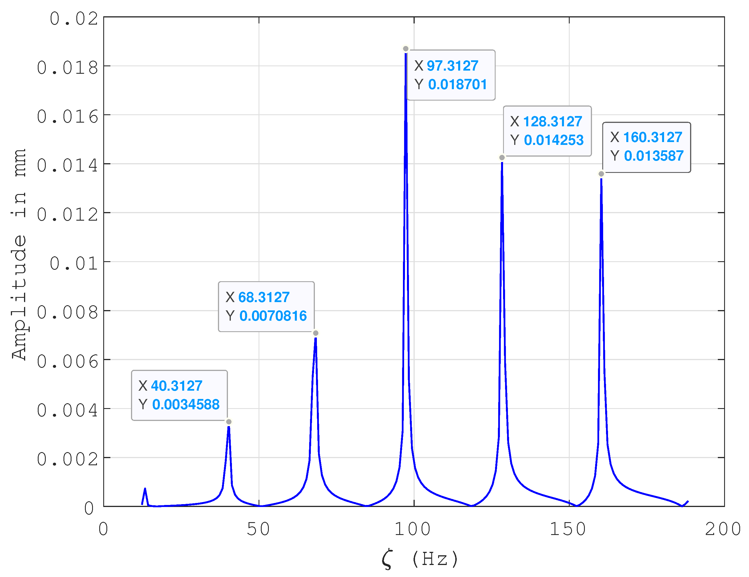
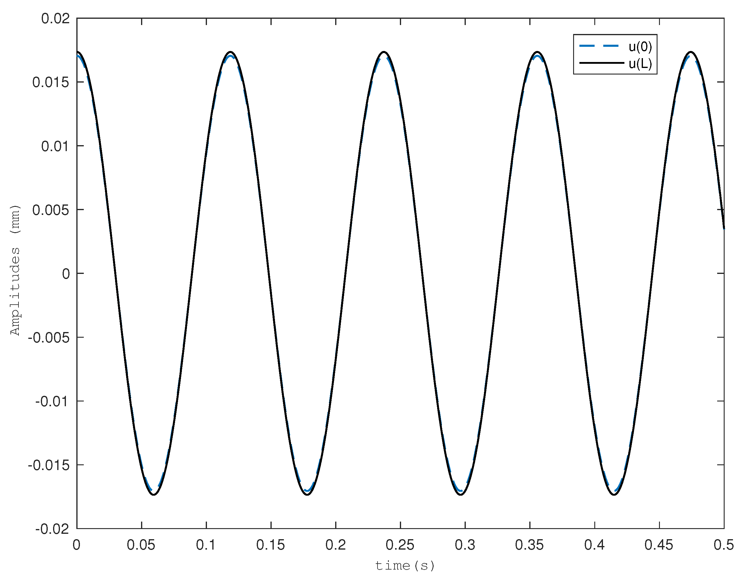
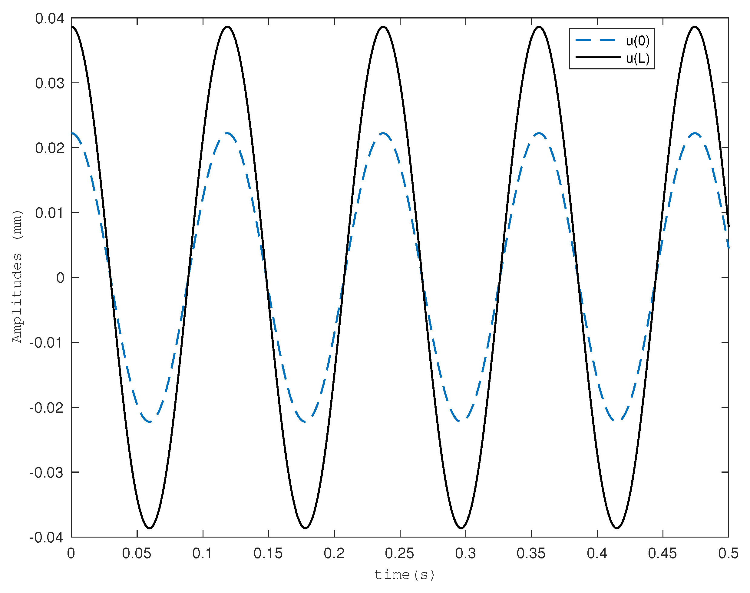
The differential operator was discretized using the Matlab Cheb/Chebfun algorithm in order to compute the associated eigenvalues [33]. Figure 2 shows the various values of the temporal frequencies that must be taken in the formulation of the eccentric masses frequency of rotation (mechanical part producing the percussion force). A maintained frequency around $\zeta =68 \mathrm{H}\mathrm{z}$ produces a practical ration ($\frac{u\left(L\right)}{u\left(0\right)}=1.73$) in the amplitude boundaries from the top to the drill bit bouncing (Figure 3) which is an equilibrium in the forces supported by devices. Figure 4 illustrates an increase in amplitude at the expense of a rather strong input amplitude which may not be provided by the system. Finally, a set of the drillstring system parameters used in the simulation is presented in Table 1.

6. Conclusions

A rigorous spectral analysis is detailed for the sonic distributed parameter drillstring dynamics where from the operator construction, formally equivalent to the abstract evolution equation in the defined Hilbert space, the problem well-posedness is proved after a semigroup formulation of the initial-boundary value problem. Details of the spectral/frequency domain analysis and the numerical operator descretization show that the input-control amplitude which is harmonic depends on an appropriate resonant mode around 68 Hz, leading to a $1.73$ ratio of amplitudes between the input/output system boundaries. Indeed, in order to complete our investigation, controlling these vibrations allows, on the one hand, the optimization of the drilling by channeling the energy along the drillstring and, on the other hand, the possibility to later engage the drilling head by a manipulator robot without fearing its malfunction. Based on this fact, a vibration model with distributed parameters has been established and its boundary control and integration represent the perspective of this work.

References

- Rockefeller, W.C. Mechanical Resonant Systems in High-Power Applications; United Engineering Center: New York, NY, USA, 1967. [Google Scholar]
- Mao, Z.X. Research on Sonic Drilling Technology Report; China University of Geosciences: Beijing, China, 2007. [Google Scholar]
- Terry, D.B. Resonant Sonic Drilling at Three Former MGP Sites: Benefits and Limitations; GEI Consultants Inc.: Woburn, MA, USA, 2003. [Google Scholar]
- Barrow, J.C. The resonant sonic drilling method: An innovative technology for environmental restoration programs. Groundw. Monit. Remediat. 1994, 14, 153–160. [Google Scholar] [CrossRef]
- Cheatham, J.B. The State of Knowledge of Rock/Bit Tooth Interactions under Simulated Deep Drilling Conditions; TerraTek Report; Bartlesville Energy Research Center, Department of Energy: Bartlesville, OK, USA, 1977. [Google Scholar]
- Sazidy, M.S.; Rideout, D.G.; Butt, S.D.; Arvani, F. Modeling Percussive Drilling Performance Using Simulated Visco-Elasto-Plastic Rock Medium; American Rock Mechanics Association: Salt Lake City, UT, USA, 2010. [Google Scholar]
- Lucon, P.A. Resonance: The Science Behind the Art of Sonic Drilling. Ph.D. Thesis, Montana State University, Bozeman, MT, USA, 2013. [Google Scholar]
- Latrach, K.; Beji, L. Axial vibrations tracking control in resonant sonic tunnel drilling system. In Proceedings of the 2015 54th IEEE Conference on Decision and Control (CDC), Osaka, Japan, 15–18 December 2015. [Google Scholar]
- Latrach, K. Vers la Robotisation Duforage sonique de Pré-soutèNement: Contrôle Frontière de Vibration Axiale. Master’s Thesis, University of Paris-Saclay, Orsay, France, 24 September 2018. [Google Scholar]
- Halsey, W.; Kyllingstad, A.; Kylling, A.; Rogaland Research Ins. Torque Feedback Used to Cure Slip- Stick Motion. In Proceedings of the SPE Annual Technical Conference and Exhibition, Houston, TX, USA, 2–5 October 1988. [Google Scholar]
- Sananikone, P. Method and Apparatus for Determining the Torque Applied to a Drillstring at the Surface. U.S. Patent 5,205,163, 27 April 1993. [Google Scholar]
- Pavone, D.R.; Desplans, J.P. Application of High Sampling Rate Downhole Measurements for Analysis and Cure of Stick slip in Drilling. In Proceedings of the SPE Annual Technical Conference and Exhibition, New Orleans, LA, USA, 25–28 September 1994. [Google Scholar]
- Jansen, J.D.; Van Den Steen, L. Active Damping of Self-excited Torsional Vibrations in Oil Well Drillstrings. J. Sound Vib. 1995, 179, 647–668. [Google Scholar] [CrossRef]
- Serrarens, A.F.A.; Van de Molengraft, M.J.G.; Kok, J.J.; Van den Steen, L. H∞ control for suppressing stick-slip in oil well drillstrings. IEEE Control. Syst. 1998, 18, 19–30. [Google Scholar]
- Tucker, W.R.; Wang, C. An Integrated Model for Drill-String Dynamics. J. Sound Vib. 1999, 224, 123–165. [Google Scholar] [CrossRef]
- Tucker, W.R.; Wang, C. On the Effective Control of Torsional Vibrations in Drilling Systems. J. Sound Vib. 1999, 224, 101–122. [Google Scholar] [CrossRef]
- Challamel, N. Rock Destruction Effect on the Stability of a Drilling Structure. J. Sound Vib. 2000, 233, 235–254. [Google Scholar] [CrossRef]
- Fridman, E.; Mondie, S.; Saldivar, B. Bounds on The Response of a Drilling Pipe Model. IMA J. Math. Control. Inf. 2010, 27, 513–526. [Google Scholar] [CrossRef]
- Saldivar, B.; Mondié, S.; Loiseau, J.J.; Rasvan, V. Stickslip Oscillations In Oilwell Drillstrings: Distributed Parameter and Neutral Type Retarded Model Approaches. In Proceedings of the 18th IFAC World Congress, Milano, Italy, 28 August–2 September 2011. [Google Scholar]
- Sagert, C.; Di Meglio, F.; Krstic, M.; Rouchon, P. Backstepping and Flatness Approaches For Stabilization of the Stick-Slip Phenomenon for drilling. IFAC Symp. Syst. Struct. Control. 2013, 46, 779–784. [Google Scholar] [CrossRef]
- Qian, Y.; Wang, Y.; Wang, Z.; Xia, B.; Liu, L. The rock breaking capability analyses of sonic drilling. J. Low Freq. Noise Vib. Act. Control. 2021, 40, 2014–2027. [Google Scholar] [CrossRef]
- Cooke, K.L.; Krumme, D.W. Differential-difference equations and nonlinear initial-boundary value problems for linear hyperbolic partial differential equations. J. Math. Anal. Appl. 1968, 24, 372–387. [Google Scholar] [CrossRef]
- Mounier, H.; Rudolph, J.; Petitot, M.; Fliess, M. A fexible rod as a linear delay system. In Proceedings of the 3rd European Control Conference, Roma, Italy, 5–8 September 1995; pp. 3676–3681. [Google Scholar]
- Balanov, A.G.; Janson, N.B.; McClintock, P.V.E.; Tucker, R.W.; Wang, C.H.T. Bifurcation Analysis of a Neutral Delay Differential Equation Modeling the Torsional Motion of a Driven Drill-string. J. Chaos Solut. Fractals 2003, 15, 381–394. [Google Scholar] [CrossRef]
- Blakely, J.N.; Corron, N.J. Experimental Observation of Delay-Induced Radio Frequency Chaos in a Transmission Line Oscillator. Chaos. J. Nonlinear Sci. 2004, 14, 1035–1041. [Google Scholar] [CrossRef] [PubMed]
- Barton, D.A.W.; Krauskopf, B.; Wilson, R.E. Homoclinic Bifurcations in a Neutral Delay Model of a Transmission Line Oscillator. J. Nonlinearity 2007, 20, 809–829. [Google Scholar] [CrossRef]
- Saldivar, B.; Knuppel, T.; Woittennek, F.; Boussaada, I.; Mounier, H.; Niculescu, S.I. Flatness-based Control of Torsional-Axial Coupled Drilling Vibrations. In Proceedings of the 19th World Congress The Inter. Federation of Automatic Control, Cape Town, South Africa, 24–29 August 2014. [Google Scholar]
- Benchikh, L.; Perpezat, D.; Beji, L.; Cascarino, S. Method of Drilling a Ground Using a Robotic Arm. Patent WO 2016/005701 A2, 14 January 2016. [Google Scholar]
- Rao, S.; Singiresu, S. Vibration of Continuous Systems; John Wiley and Sons, Inc.: Hoboken, NJ, USA, 2007. [Google Scholar]
- Prüss, J. On the spectrum of C0-semigroups. Trans. Am. Math. Soc. 1984, 284, 847–857. [Google Scholar]
- Huang, F. Characteristic conditions for exponential stability of linear dynamical systems in Hilbert space. Ann. Differ. Equ. 1985, 1, 43–45. [Google Scholar]
- Brezis, H. Analyse Fonctionnelle. In Théorie et Applications; Masson: Paris, France, 1992. [Google Scholar]
- Abell, M.L.; Braselton, J.P. Differential Equations with Maple V; Academic Press: Cambridge, MA, USA, 1994. [Google Scholar]
Figure 2.
Drillstring sonic drill model frequency response.
Figure 3.
Amplitudes for and for Hz.
Figure 4.
Amplitudes for and for = 73 Hz.