Prediction of ECOG Performance Status of Lung Cancer Patients Using LIME-Based Machine Learning

Abstract

The Eastern Cooperative Oncology Group (ECOG) performance status is a widely used method for evaluating the functional abilities of cancer patients and predicting their prognosis. It is essential for healthcare providers to frequently assess the ECOG performance status of lung cancer patients to ensure that it accurately reflects their current functional abilities and to modify their treatment plan accordingly. This study aimed to develop and evaluate an AdaBoost classification (ADB-C) model to predict a lung cancer patient’s performance status following treatment. According to the results, the ADB-C model has the highest “Area under the receiver operating characteristic curve” (ROC AUC) score at 0.7890 which outperformed other benchmark models including Logistic Regression, K-Nearest Neighbors, Decision Trees, Random Forest, XGBoost, and TabNet. In order to achieve model prediction explainability, we combined the ADB-C model with a LIME-based explainable model. This explainable ADB-C model may assist medical professionals in exploring effective cancer treatments that would not negatively impact the post-treatment performance status of a patient.

1. Introduction

As the field of big data continues to evolve, healthcare (disease management and health prediction) is shifting its paradigm to precision medicine, custom medicine, and participatory medicine focusing on the characteristics and participation of individual patients [1]. For effective treatment/intervention using health promotion, health care, disease prevention, and customized medicine, in particular, accurate prediction models based on reliable medical/healthcare big data are crucial [2,3]. In recent years, the use of medical big data has been actively carried out in the field of early diagnosis, intervention, and treatment of cancer [4,5]. Developing a prognosis model to predict a patient’s performance status after receiving treatment is critical for all-round customized treatments in cancer patients.

Lung cancer is not only one of the most prevalent cancers worldwide, but it also ranks the second among the causes of cancer-related deaths [6]. In South Korea, the 5-year survival rate for lung cancer patients was 32.4% (duration 2014–2018) [7], a cancer type with a low survival rate. However, with the recent expansion of health check-ups, the chances of a complete cure are increasing through early diagnosis, and the survival period is being continuously extended with the advancement of chemotherapy and radiation therapy [8]. In patients with lung cancer, functional status is a critical factor that can not only predict prognosis, but also determine the quality of life [9]. It has been reported that functional status is closely linked to symptom experience, meaning that as symptoms become more severe, functional abilities decline [10]. To extend the survival of lung cancer patients and enhance their quality of life, it is crucial to implement systematic symptom management led by health professionals.

The ECOG Performance Status Scale (ECOG PS) [11,12], which was developed by the Eastern Cooperative Oncology Group, is a widely used method for evaluating the functional abilities of cancer patients and predicting their prognosis. There are various factors that can influence the ECOG PS of lung cancer patients, including age, tumor stage, comorbid conditions, treatment side effects, psychological factors, and physical symptoms [13]. It is crucial to remember that the ECOG PS is not a permanent measurement and can alter as the patient’s health status and treatment evolve. Therefore, it is important for healthcare providers to frequently assess the ECOG PS of lung cancer patients to ensure that it accurately reflects their current functional abilities and to modify their treatment plan accordingly.

According to recent studies, classification is the most often used machine-learning (ML) problem in the medical industry [14], and solutions based on AdaBoost (ADB) [15] algorithm make up a sizeable portion of the study. Applications in clinical medicine include the detection of diseases such as diabetes, hypertension, Alzheimer’s disease, and various malignancies [16,17,18,19]. Non-clinical evaluations of subhealth status and self-reported mental health are also applied [20,21]. Additionally, ADB has been employed as a preprocessing technique for automatically picking out the feature importance of high-dimensional data [22,23]. Nevertheless, ADB is regarded as a typical black box due to its internal structure: an ensemble of often hundreds to thousands of shallow decision trees. The ensemble classifies data instances using a weighted majority vote, which is challenging to analyze numerically. Despite its wide use in medicine, ADB persists as a black box; thus, explaining how it works remains difficult.

The recently developed framework known as local interpretable model-agnostic explanation (LIME) may be used with any black-box classification model to generate an explanation for a singular manifestation [24]. This technique finds the fewest features that most strongly influence the likelihood of a single-class outcome for a single observation while also presenting a local explanation for the classification. Therefore, LIME can explain the AdaBoost, or any other black-box machine learning models, to provide interpretable explanations of the model’s behavior around individual instances. LIME has been evaluated for use in numerous medical applications [25,26,27] due to its accelerated capacity to generate explanations.

In this research, we aim to develop and evaluate an ADB-based prognosis model that could help medical professionals consider the ECOG PS of lung cancer patients when receiving treatment options. As a result, we provide a hybrid model for predicting a cancer patient’s ECOG PS following treatment, which combines a LIME-based explainability model with the ADB model. The combined model can explain the ADB classifier’s predictions properly and comprehensively. To evaluate the model’s performance, we compare the ADB model with other machine learning models, including Logistic Regression (LR), K-Nearest Neighbors, Decision Trees (DT), Random Forest (RF) and XGBoost (XGB). We also compared our old traditional model with a TabNet classification model, a recently released explainability deep learning model that outperforms several prediction models on tabular data. We hope that our explainability model might assist medical professionals in exploring effective cancer treatments that would not negatively impact the post-treatment ECOG PS of a patient.

The construction of this research paper is as follows: In Section 2, a related background study is discussed with proper explanations and results. Section 3 presents the materials and methods of our research. Section 4 includes the results of our prediction model and relevant discussions. Section 5 points out the limitations and future plans of this study. In the final section, we outline our concluding remarks.

2. Background Study

Clinical data for lung cancer and the ADB model interact exceptionally effectively in previous research studies [28,29,30]. The earlier studies listed below demonstrate the ADB’s excellent performance in terms of predicting lung cancer or survival of lung cancer. Despite the fact that research on the ADB model to predict cancer patient ECOG PS is lacking, these studies used lung cancer clinical datasets that are quite similar to ours. As a result, we decided to include the ADB model in our research for a successful outcome.

Ingle et al. [28] utilized AdaBoost algorithm to predict different lung cancer types. The proposed model was trained with features extracted from lung CT images. The AdaBoost model outperformed the Decision Tree, Random Forest, and K-Nearest Neighbors, with 90.74% accuracy, 81.8% sensitivity, 93.9% specificity, 0.8 F1 score, and 0.93 ROC AUC.

Using several machine learning models, Sim et al. [29] presented research on health-related quality of life (HRQOL) in the 5-year survival of lung cancer prediction model. The performance of the models was assessed by k-fold 5 cross-validation into two different feature sets using AdaBoost, Bagging, Decision Tree, Random Forest, and Logistic Regression. The performance of the model was compared to the clinical (HRQOL) data of 809 lung cancer surgery survivors. The results showed that AdaBoost and Random Forest outperformed the other models. The best accuracy was attained by AdaBoost, with 94.8 and 94.9% of AUC.

For predicting lung cancer survival, Safiyari et al. [30] employed a variety of ensemble learning techniques, including Bagging, MultiBoosting, AdaBoost, Dagging, and Random SubSpace. They also used Logistic Regression, Random Forest, Bayes Net, SMO, Decision Stump, C4.5, Simple Cart, and RIPPER. The authors assessed the prediction model using the undersampling technique on the Surveillance, Epidemiology, and End Results (SEER) dataset containing 643,924 samples and 149 variables. AUC and accuracy metrics for AdaBoost were found to be 94.9% and 88.98%, respectively, better than other competing methods.

3. Materials and Methods

3.1. Materials

At the Korean Central Cancer Registry, there were 2829 cases of lung cancer reported nationwide in 2016. The Korean Association for Lung Cancer and Korean Central Cancer Registry chose data using a systematic sampling method for initial analysis in order to investigate the specific clinical characteristics, treatment information, and outcomes of Korean lung cancer patients (13 national or regional cancer centers) [31]. Gender, age, smoking history, body mass index, performance status, histopathologic type, symptoms, clinical stage (determined by the seventh edition of the TNM International Staging System), ECOG PS, treatment method, and survival status were all collected in accordance with a standardized protocol [32]. Telephone interviews, medical records, and the database of the National Health Insurance (NIH) of Korea were used to gather survival data for every patient. The Institutional Review Board at the National Cancer Center (NCC) examined and approved the study protocol. Due to this study’s retrospective nature, informed consent was waived. In this study, we finally analyzed the clinical data of 2063 lung cancer patients.

3.2. Data Preprocessing

Preprocessing of the dataset was necessary before the model could be fitted. There were a total of 2829 patients and 328 columns of identifying information in the raw data collection. In the beginning, we eliminated 18 redundant columns relating to the serial number and date/time values. The dataset’s categorical variables were then encoded using label encoding. In this study, the “ECOG” column, which stands for ECOG PS, was selected as the target variable.

To account for missing values, columns containing 50% null values and rows with missing values on “ECOG” were removed from the dataset. Since this dataset included both numerical and categorical variables, we combined the forward-fill (ffill) and back-fill (bfill) techniques to fill in the remaining null values with values from the columns that were not empty. After deleting unnecessary columns and addressing missing values, the dataset was reduced to 2063 patients with 286 variables and the target feature. The dataset was divided into two sets, one for training and one for testing, with an 80:20 split, in order to complete the essential setup for the model to learn.

As indicated previously, the target feature “ECOG” refers to the Eastern Corporative Oncology Group score, which measures a patient’s level of functioning in terms of self-care, daily activities, and physical capabilities.

Table 1. ECOG Performance Status Scale and the number of each score values in the dataset.

Score	ECOG Performance Status	Number of Values
0	Fully active, able to carry on all pre-disease performance without restriction	904
1	Restricted in physically strenuous activity but ambulatory and able to carry out work of a light or sedentary nature, e.g., light house work, office work	888
2	Ambulatory and capable of all self-care but unable to carry out any work activities; up and about more than 50% of waking hours	164
3	Capable of only limited self-care; confined to bed or chair more than 50% of waking hours	73
4	Completely disabled; cannot carry on any self-care; totally confined to bed or chair	34
5	Dead	0

displays each score’s precise definition as well as how many values of each score there are overall in the dataset. As shown in Table 1, the number of score 0 is excessively out of proportion to the other scores. This imbalanced data may cause machine learning models to overfit during the prediction phase. We opted to aggregate values of scores from 1 to 5 into one group signifying “limited in physical activity,” encoded as value 1, in order to manage the unbalanced problem without changing the dataset’s size. The value and significance of score 0 remain unchanged. After processing, only two values were present in the “ECOG” column: 0 = fully active and able to execute all pre-disease functions without limitation; 1 = physical activity restricted. The ratio between the number of score 0 values (class 0) and the number of score 1 values (class 1) is 904:1159

3.3. Feature Selection

Feature selection is crucial before developing machine learning models. Feature selection methods help identify and prioritize the most critical and highly regarded features included in a dataset. There are three approaches to selecting features: wrapper, filter, and embedded method [33]. The embedded method is an intermediate option between the filter method and the wrapper method because the embedded method includes the qualities of both methods [34]. In particular, the embedded technique is computationally simpler than the wrapper method while still being more computationally intensive than the filter method. This reduced computational burden occurs despite the fact that the embedded method permits interactions with the classifier (i.e., it incorporates the classifier’s bias into feature selection, which tends to improve classifier performance) in the same manner as wrapper methods.

In an embedded technique, feature selection is incorporated or built into the classification algorithm. The classifier modifies its internal settings and chooses the proper weights/importance given to each feature to generate the greatest classification accuracy during the training phase. As a result, in an embedded method, the process of finding the ideal feature subset and building the model are combined into a single step [35].

In this research, the ADB, RF, and XGB models, which have their own built-in feature selection methods, are examples of embedded methods. Consequently, we selected important features from the dataset using the feature selection procedures of the corresponding models. In addition, we utilized the ExtraTree (ET) model [36], a variant of Random Forests with more randomization at each stage for selecting an optimal cut/split or decision boundary, to select essential features. In contrast to Random Forests, where features are divided based on a score (such as entropy) and instances of the training set are bootstrapped, the ET split criteria are random, and the entire training set is considered. The resulting trees have more leaf nodes and are more computationally efficient. Due to its randomization, the ET algorithm also alleviates the problem of high variance in Random Forests and thus provides a superior bias-variance trade-off. In this study, we employed the default models of RandomForestClassifier, ExtraTreeClassifier, XGBClassifier, and AdaBoostClassifier from the sklearn library in Python version 3.11.3 to fit the training set, then selected features with an importance score of 0.01 or higher.

3.4. Development of ML Models

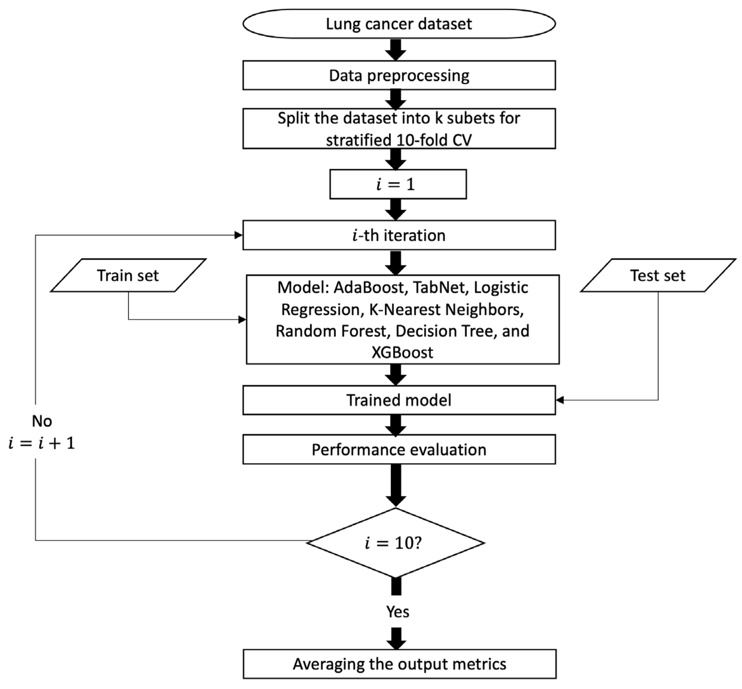
All classification experiments were developed by using the Python programming language. An overview of the model pipeline is graphically depicted in Figure 1. In our research, machine learning models were evaluated using the stratified 10-fold cross-validation (CV) method. When utilizing a k-fold CV, the dataset is divided into k equal-sized sections, and cases are randomly chosen for each fold. A portion of each subset is utilized for testing, while the remaining portion serves as the training set. Each subset is utilized as the test set once during the k evaluations of the model. During a stratified k-fold cross-validation, each subset is divided into groups with about the same class labels as the original dataset.

3.4.1. AdaBoost Classification (ADB-C) Model

A classification task is a traditional learning issue that may be expressed as a search for a good classifier/classification rule, h, utilizing given data $\{x_i,y_i\},i=\mathrm{1,2},...,m$. In this case, $x$ is a vector of $m$ predictors, and the class of the pattern associated with $x$ is shown by $y$, which takes the values $\{-1,1\}$. When a classifier’s error rate is only marginally better than random guessing, we call it a weak classifier, and when it is significantly better than random guessing, we call it a strong classifier.

In the majority of instances, it may be challenging to attain adequate accuracy using a single classifier [37]. Numerous methods, such as noise injection, might be utilized to strengthen a weak classifier by stabilizing its decision [38]. A different strategy is to build several weak classifiers instead of just one and combine them to create a powerful classifier. Many of these combining approaches have recently been created, and Freund and Schapire’s ADB algorithm is one of the more well-known and efficient ones [39]. ADB aims to discover a highly accurate classifier by merging a large number of weak classifiers, each of which may be just moderately accurate [40,41,42]. The core concept behind the ADB method is to construct a unique probabilistic distribution of learnable patterns (the training set), based on prior outcomes, at each step (for each classifier). Each design has a weight assigned to it. It is initially set to $1/m$, and at each step, the weight of each pattern that was incorrectly categorized is increased (or conversely, the weight of each sample that was properly classified is dropped), focusing the new classifiers on complicated patterns. This allows for the training of a chain of training sets and classifiers. As a result, the final decision can be reached by a weighted majority vote. The concept of the ADB algorithm includes the following steps:

Given: $\left(x_1,y_1\right),\dots .,(x_m,y_m)$ where $x_i\in \mathcal{X},y_i\in \{-1,1\}$.

Initialize: $D_1\left(i\right)=\frac{1}{m} for i=1,\dots .,m.$

For $t=1,\dots .,T$:

• Train weak learner using distribution $D_t$;
• Get weak hypothesis $h_t:\mathcal{X}\to \{-1,1\}$;
• Aim: select $h_t$ with low weighted error:

  $${\epsilon }_t={Pr}_{i-D_t}[h_t\left(x_i\right)\ne y_i]$$
• Choose ${\alpha }_t=\frac{1}{2}ln\left(\frac{1-{\epsilon }_t}{{\epsilon }_t}\right)$;
• Update, for i = 1, …, m:

  $$D_{t+1}\left(i\right)=\frac{D_1\left(i\right)exp(-{\alpha }_t{y}_i{h}_t{(x}_i))}{Z_t}$$

  where Zt is a normalization factor (chosen so that Dt + 1 will be a distribution).

Output the final hypothesis:

$$H(x)=sign({\sum }_{t=1}^T{\alpha }_t{h}_t(x))$$

(1)

In this study, we used sklearn library in Python to build the ADB-C model. For fine-tuning hyper-parameters of the model, we used Optuna library, an automated search for optimal hyperparameters framework using Python [43].

3.4.2. TabNet Classification (TN-C) Model

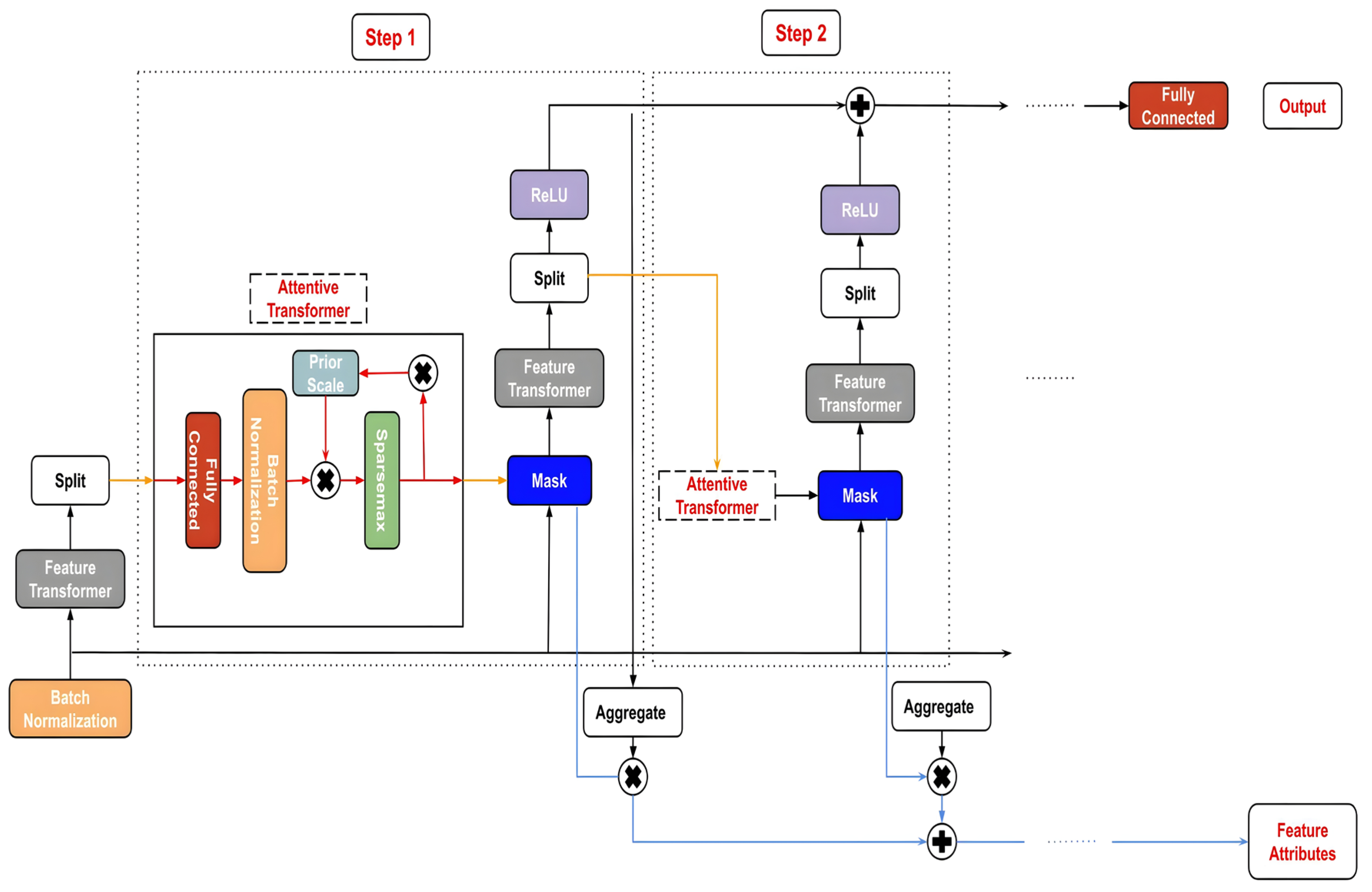
TabNet (TN) is a deep learning model that is constructed on the foundation of sequential multistep processing [44]. TN’s architecture enhances the ability to learn high-dimensional features and helps in feature selection. Each nth stage generates an output for a Feature Transformer block after processing a d-dimensional feature vector. This feature transformer block has several levels that are either common to all decision steps or specific to a certain decision step. A batch normalization layer, a Gated Liner Unit (GLU) activation, and fully linked layers are all present in every block. The GLU also has a link to a normalization residual connection, which reduces the variation over the whole network. This multi-layered block improves the parameter efficiency of the network and aids in feature selection.

A thorough explanation of the TN’s architecture is given in Figure 2. An attentive transformer, mask, feature transformer, split node, and ReLu activation are all included in each phase. Before connecting to a fully linked layer and the output, the steps are sequentially increased by up to N steps. A fully linked layer, batch normalization, prior scaling, and sparsemax dimensionality reduction are all included in Attentive Transformer. Significant feature contributions for aggregation are produced using the mask function.

The TN-C model in this research was built by pytorch_tabnet version 4.0. The hyper-parameters inside model were also fine-tuned by Optuna framework.

3.4.3. Performance Comparison with Other Machine Learning Models

Five machine learning models, including Logistic Regression [45], K-Nearest Neighbors [46], Random Forest [47], Decision Tree [48], and XGBoost [49], are used as benchmarks for comparison in order to validate the prediction performance of the proposed method. These techniques have been applied to the field of lung cancer prediction and ECOG PS prediction with positive outcomes [28,29,50]. The same training and test sets are used for all models’ evaluations. Notably, the Optuna framework also yields the optimal settings for these benchmarks.

3.5. Model Evaluation

After the implementation models, evaluating the proposed ML models’ performance is an important step. The most often used terminology for a binary classification test are precision, recall, and F1-score, which all offer statistical evaluation of the performance of a classifier model. These metrics were calculated as follows:

• Accuracy estimates the number of positive and negative events that are accurately classified.

Accuracy = (True_positive + True_negative)/(True_positive + True_negative + False_positive + False_negative)

(2)

• Precision is defined as the proportion of positive cases that are actually positive.

Precision = True_positive/(True_positive + False_positive)

(3)

• Recall is the proportion of positive cases that are predicted to be positive out of all positive instances.

Recall = True_positive/(True_positive + False_negative)

(4)

• F1 score is the harmonic mean of precision and recall.

F1 score = 2 × (Precision × Recall) × (Precision + Recall)

(5)

Additionally, we also utilized “Area under the receiver operating characteristic curve value” (ROC AUC) to assess the model’s performance. An AUC summarizes a model’s overall diagnostic test accuracy, whereas a ROC curve plots the True Positive Rate (TPR) versus the False Positive Rate (FPR) of a diagnostic test. The range of the ROC AUC metric is [0, 1], with 0 signifying a completely erroneous result, 0.5 meaning the classifier is unable to distinguish between positive and negative class outcomes, 0.7–0.8 being rated good, 0.8–0.9 being deemed great, and >0.9 being regarded as outstanding. The ROC AUC is defined as follows:

$$ROC AUC={\int }_1^{0}TPR\left(t_i\right)d\left(FPR\left(t_i\right)\right)$$

(6)

where $TPR\left(t_i\right)$ and $FPR\left(t_i\right)$ denote the true positive rate and false positive rate for a threshold $t_i$.

In our investigation, it was assumed that a model with the greatest ROC AUC had the best predictive capacity. If the ROC AUC remained stable, the model with the highest recall was considered the best.

3.6. Local Interpretable Model-Agnostic Explanations (LIME)

LIME [24] usability and clarity are its most intriguing features. This strategy aims to use an interpretable representation of the input data that is simple enough for humans to understand [51]. As a result, the output of LIME is a set of explanations that emphasizes how each characteristic contributed to the prediction of a data sample. LIME repeatedly perturbs an observation to produce duplicated feature data in order to explain it [51]. The prediction model is then used to generate predictions on the altered data. Following this, each data point in the perturbed data is compared to the original data point of the dataset, and the Euclidean distance between the two points is calculated to indicate the distance between the disturbed data point and the original observation. This provides an indication of which input features the model deems most relevant for making predictions.

The fundamental objective is to provide an explanation that is trustworthy and understandable. In order to do this, LIME minimizes the subsequent objective function as follows:

$$\xi \left(x\right)={argmin}_{g\in G}\mathcal{L}(f,g,{\pi }_x)+\Omega \left(g\right)$$

(7)

where $f$ is the original model, g is the interpretable model, $x$ represents the original observation, ${\pi }_x$ denotes the proximity measure from all permutations to the original observation, $\mathcal{L}(f,g,{\pi }_x)$ component is a measure of unfaithfulness of $g$ in approximating $f$ in the locality defined by π, and $\mathsf{\Omega }\left(g\right)$ is a measure of model complexity.

4. Results

4.1. Feature Selection Results

After retrieving important features selected by RF, ET, XGB, and ADB embedded methods, we employed the default ADB-C, LR, XGB, KNN, DT, and TN-C models to evaluate the effectiveness of feature selection methods. The comparison results are shown in

Table 2. Performance comparison of feature selection methods.

Features Set	Model	Accuracy	Precision	Recall	F1-Score	ROC AUC
All features	RF	0.7369	0.7329	0.8385	0.7818	0.7726
	XGB	0.7085	0.7268	0.7743	0.7490	0.7531
	ADB-C	0.7078	0.7256	0.7743	0.7486	0.7488
	LR	0.7036	0.7099	0.8014	0.7524	0.7369
	TN-C	0.6905	0.6781	0.8768	0.7608	0.7186
	KNN	0.6219	0.6589	0.6782	0.6679	0.6526
	DT	0.6372	0.6784	0.6732	0.6755	0.6321
RF feature selection	ADB-C	0.7050	0.7173	0.7866	0.7496	0.7481
	RF	0.7112	0.7202	0.7965	0.7560	0.7457
	LR	0.6961	0.7015	0.8002	0.7472	0.7323
	XGB	0.6974	0.7157	0.7682	0.7400	0.7306
	KNN	0.6427	0.6724	0.7139	0.6920	0.6591
	TN-C	0.6537	0.6470	0.8495	0.7334	0.6583
	DT	0.5921	0.6413	0.6251	0.6323	0.5875
ET feature selection	ADB-C	0.7071	0.7257	0.7731	0.7478	0.7663
	RF	0.7168	0.7232	0.8088	0.7625	0.7619
	XGB	0.7057	0.7267	0.7669	0.7453	0.7460
	LR	0.7085	0.7128	0.8076	0.7561	0.7410
	TN-C	0.6482	0.6454	0.8383	0.7272	0.6681
	KNN	0.6295	0.6591	0.7078	0.6820	0.6495
	DT	0.6233	0.6705	0.6548	0.6613	0.6188
XGB feature selection	LR	0.7237	0.7097	0.8619	0.7779	0.7531
	ADB-C	0.7230	0.7093	0.8606	0.7773	0.7523
	XGB	0.7244	0.7098	0.8631	0.7786	0.7479
	RF	0.7216	0.7096	0.8557	0.7755	0.7466
	KNN	0.6981	0.7441	0.7167	0.7151	0.7399
	DT	0.7209	0.7124	0.8459	0.7730	0.7378
	TN-C	0.7182	0.7073	0.8533	0.7728	0.7253
ADB feature selection	ADB-C	0.7230	0.7325	0.8002	0.7645	0.7795
	RF	0.7237	0.7314	0.8076	0.7670	0.7774
	LR	0.7140	0.7252	0.7916	0.7565	0.7666
	XGB	0.6994	0.7200	0.7620	0.7395	0.7536
	TN-C	0.6614	0.6502	0.8742	0.7433	0.6738
	KNN	0.6213	0.6653	0.6597	0.6610	0.6490
	DT	0.6385	0.6840	0.6609	0.6710	0.6353

AdaBoost Classification model = ADB-C, Logistic Regression model = LR, TabNet Classification model = TN-C, XGBoost Classification model = XGB, Random Forest Classification model = RF, K-Nearest Neighbors Classification model = KNN, Decision Tree Classification model = DT.

. When using all features, the default RF model had a ROC AUC of 0.7726, which was superior to the top models using RF feature selection, ET feature selection, and XGB feature selection. In the case of utilizing feature selection methods, the default ADB-C model outperformed the majority of the methods in terms of ROC AUC score. The default ADB-C model obtained the highest ROC AUC (0.7795), particularly when using features selected by the ADB feature selection method. In this study, out of 286 variables, only 35 features chosen by the ADB feature selection method were used to determine and optimize the optimal prediction model.

Table 3. Variables and their description.

Variables	Description	Field Type
age	Age	Continuous: ( ) years old
DLCO	Carbon monoxide diffusing capacity (DLCO)	Continuous: ( ) mL/min/mmHg
FVC	Forced vital capacity (FVC)	Continuous: ( ) L
FEV1	The first second of forced expiration (FEV1)	Continuous: ( ) L
HC_T	Tumor stage	Categorical: Tx (0), T1a (1), T1b (2), T1 NOS (3), T2a (4), T2b (5), T2 NOS (6), T3 (7), T4 (8), Unknown (9)
HC_MAXSIZE	Tumor maximal size	Continuous: ( ) cm
DLCO_PERCENT	DLCO percent predictive value	Continuous: ( )%
H_METHOD_8	Bx from distant metastasis (liver, adrenal, bone, brain, skin, etc.)	Categorical: No (0), Yes (1)
H_METHOD_11	Other diagnosis method	Categorical: No (0), Yes (1)
H_NAME_5	Small cell carcinoma	Categorical: No (0), Yes (1)
OP_NAME_9	Other operation approach	Categorical: No (0), Yes (1)
HC_NSITE1_1	Hilar lymph nodes (#10) in clinical 1 stage	Categorical: No encroachment (0), Encroachment (1)
gender	Gender	Categorical: Male (1), Female (2)
OP_APPROACH_1	Thoracotomy/Open operative approach	Categorical: No (0), Yes (1)
OP_APPROACH_3	Mediastinum operative approach	Categorical: No (0), Yes (1)
MED3_REG_CODE_5	Paclitaxel	Categorical: Not use (0), Use (1)
MED3_REG_CODE_27	Durvalumab	Categorical: Not use (0), Use (1)
HC_MSITE2_2	Extra thoracic lymph node	Categorical: No (0), Metastasis (1)
HC_MSITE1_1	Malignant pleural effusion	Categorical: No (0), Yes (1)
S_NAME_1	Squamous cell carcinoma	Categorical: No (0), Yes (1)
MED1_REG_CODE_15	Crizotinib	Categorical: No (0), Yes (1)
HC_NSITE2_3	Lower paratracheal lymph nodes (#4) in clinical 2 stage	Categorical: No encroachment (0), Encroachment (1)
HC_NSITE3_11	Lobar lymph node	Categorical: No encroachment (0), Encroachment (1)
H_METHOD_4	Lymph node needle aspiration and/or biopsy	Categorical: No (0), Yes (1)
TREAT_S	Surgery	Categorical: No (0), Yes (1)
REASON	Reason	Categorical: Symptoms (1), Incidental discovery (abnormal findings on chest imaging) (2), Unknown (9)
PFT	Pulmonary function test performed	Categorical: No (0), Yes (1)
TX_COM_2	Radiation therapy	Categorical: No (0), Yes (1)
S_LOCATION_1	Tumor is located in right upper lobe	Categorical: No (0), Yes (1)
TX_COM	Treatment carried out in the hospital	Categorical: No (0), Yes (1), Last month (2), Unknown (9)
SYMPTOMS_9	Other symptoms	Categorical: No (0), Yes (1)
WEIGHT	Weight	Continuous: ( ) kg
SYMPTOMS_8	Pain (chest, head, spine, abdomen, extremity)	Categorical: No (0), Yes (1)
HEIGHT	Height	Continuous: ( ) cm
SYMPTOMS_4	Dyspnea	Categorical: No (0), Yes (1)

provides details on the 35 variables.

4.2. Performances of ADB-C Model and TN-C Model

After identifying the key characteristics to train in the ML models, only 2063 patients and 35 variables remained in our dataset. As a result, the dataset was not excessively large. In order to achieve the ideal models, we might thus employ a wide search space to fine-tune the hyperparameters of the ADB-C and other benchmark models. We optimized the hyper-parameters of both the ADB-C model and other benchmark models by Optuna, and the optimal hyper-parameters for each model are as follows:

• ADB-C: ‘algorithm’: ’SAMME’, ‘learning_rate’: 0.9871, ‘n_estimators’: 727.
• TN-C: ‘mask_type’: ‘entmax’, ‘n_da’: 64, ‘n_steps’: 6, ‘gamma’: 1, ‘n_shared’: 4, ‘lambda_sparse’: 2.53e-06, ‘bn_momentum’: 0.9997, ‘patienceScheduler’: 10, ‘patience’: 24, ‘epochs’: 92, ‘optimizer_fn’: ‘torch.optim.adam.Adam’.
• LR: ‘C’: 2.3567, ‘max_iter’: 452
• KNN: ‘n_neighbors’: 19, ‘weights’: ‘distance, ‘p’: 1.
• DT: ‘criterion’: ‘gini’, ‘splitter’: ‘best’, ‘max_depth’: 5, ‘min_samples_split’: 8, ‘min_samples_leaf’: 1, ‘max_features’: ‘sqrt’.
• XGB: ‘learning_rate’: 0.0259, ‘n_estimators’: 393, ‘max_depth’: 3, ‘subsample’: 0.6381, ‘colsample_bytree’: 0.365.

In our dataset, the ROC AUC of the ADB-C model was the best. In details, ADB-C model had ROC AUC = 0.7890, while LR had ROC AUC = 0.7863, and XGB model had ROC AUC = 0.7859. RF, DT, and TN-C had ROC AUC of 0.7817, 0.7343, and 0.7242, respectively. The ROC AUC was only 0.7180 for the KNN model, which was the lowest. Other performance scores are displayed in

Table 4. Performance of optimized prediction models.

Model	Accuracy	Precision	Recall	F1-Score	ROC AUC
ADB-C	0.7223	0.7274	0.8126	0.7671	0.7890
LR	0.7258	0.7330	0.8051	0.7670	0.7863
XGB	0.7300	0.7384	0.8064	0.7703	0.7859
RF	0.7334	0.7333	0.8286	0.7775	0.7817
DT	0.7029	0.7337	0.7448	0.7371	0.7343
TN-C	0.6475	0.6852	0.6118	0.5879	0.7242
KNN	0.6732	0.7075	0.7152	0.7106	0.7180

AdaBoost Classification model = ADB-C, Logistic Regression model = LR, TabNet Classification model = TN-C, XGBoost Classification model = XGB, Random Forest Classification model = RF, K-Nearest Neighbors Classification model = KNN, Decision Tree Classification model = DT.

. As can be observed, the ADB-C model outscored other models on ROC AUC and accuracy. Moreover, the ADB-C model had a good recall score (0.8126). This also suggests that our model is exceptionally good at predicting true positive cases in the total number of positive cases (patients with physical activity restrictions).

4.3. Evaluation of LIME-Based Stacking Ensemble Model

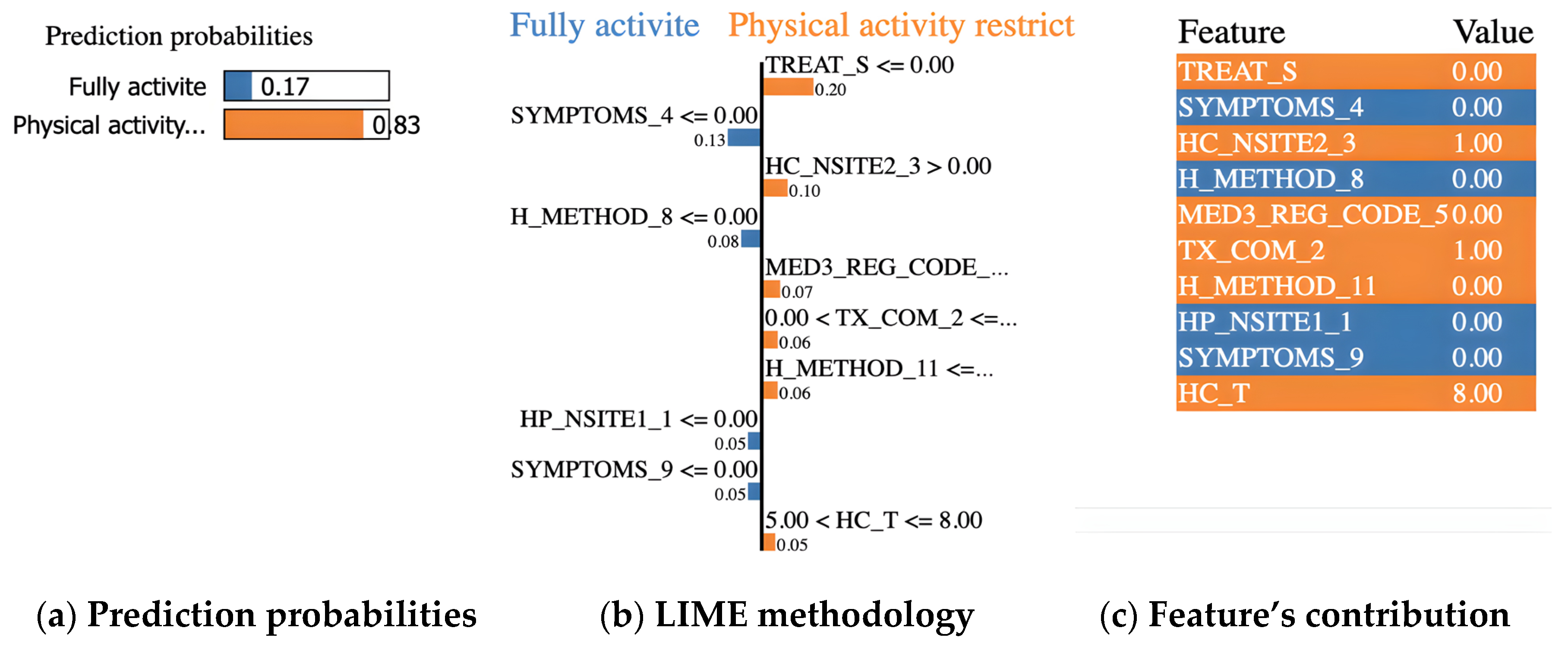
We chose a specific instance to analyze in order to show how the LIME model works with the ADB-C model to predict a cancer patient’s ECOG PS following treatment. Figure 3 depicts a description of a lung cancer patient with physical activity restricted. Figure 3c summarizes the patient’s state and contributing circumstances. We summarized the states of a patient by 10 features with the most impact in a total of 35 variables as listed below:

• TREAT_S = 0 (surgery in the past: no)
• SYMPTOMS_4 = 0 (dyspnea: no)
• HC_NSITE2_3 = 1 (lower paratracheal lymph nodes (#4) in clinical 2 stage: encroachment)
• H_METHOD_8 = 0 (Bx from distant metastasis (liver, adrenal, bone, brain, skin, etc.): no)
• MED3_REG_CODE_5 = 0 (paclitaxel: not use)
• TX_COM_2 = 1 (radiation therapy: yes)
• H_METHOD_11 = 0 (other diagnosis method: no)
• HP_NSITE1_1 = 0 (hilar lymph nodes (#10) in clinical 1 stage: no)
• SYMPTOMS_9 = 0 (other symptoms: no)
• HC_T = 8 (tumor stage: T4)

Our ADB-C model predicted that the patient would have physical activity restricted with a probability of 83%, as shown in Figure 3a. Figure 3b depicts the LIME methodology. The blue bars represent the variables that significantly contribute to the prediction’s rejection, whereas the orange bars represent the states and factors that considerably contribute to the prediction’s support. According to the explanation, at the time of the prediction, “Surgery (TREAT_S), Lower paratracheal lymph nodes (#4) in clinical 2 stage (HC_NSITE2_3), Paclitaxel (MED3_REG_CODE_5), Radiation therapy (TX_COM_2), Other diagnosis method (H_METHOD_11), and Tumor stage (HC_T)” were the target’s main factors and states that most contribute to the prediction of physical activity restricted patient.

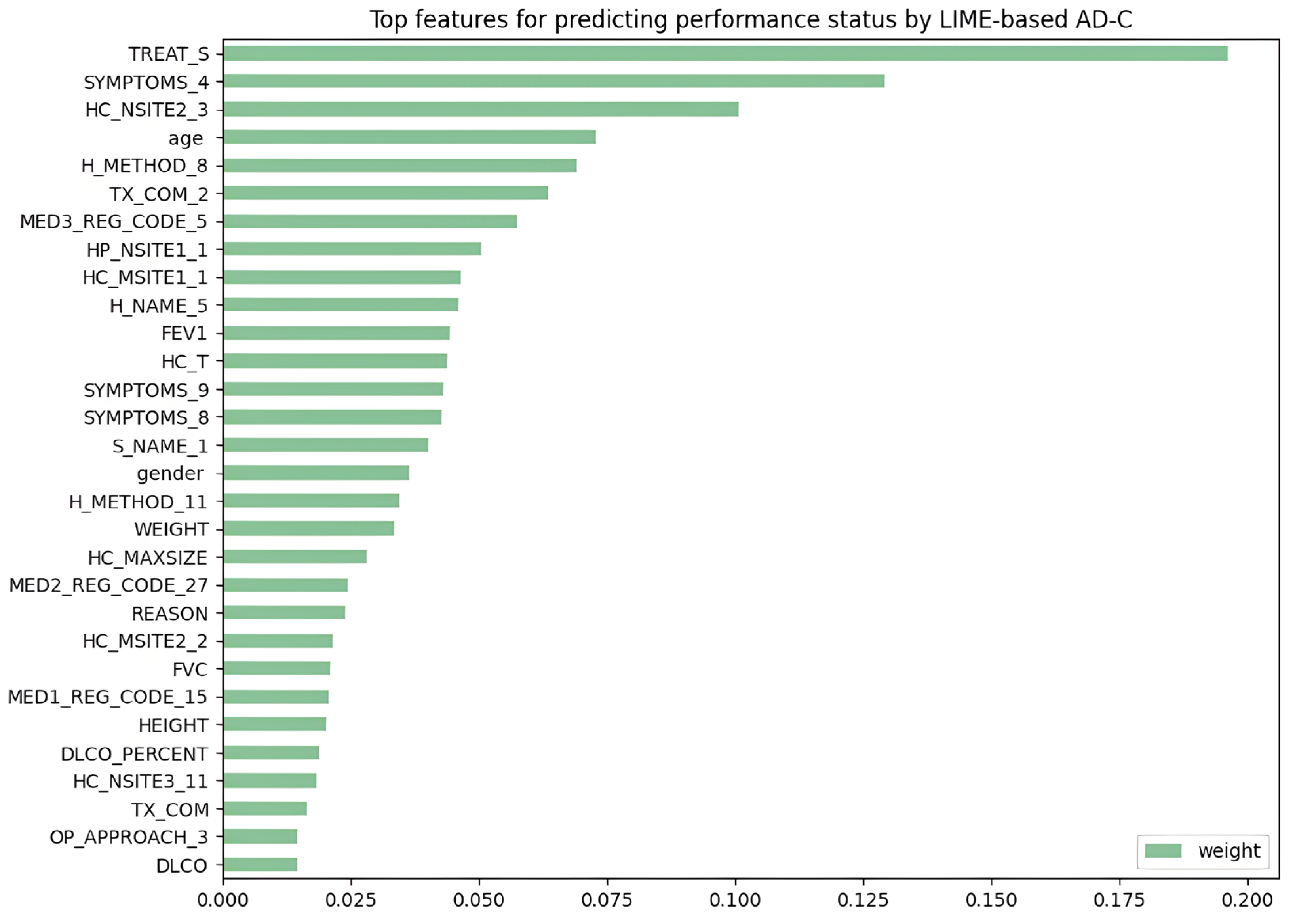
After applying LIME to all testing data in cases of a lung cancer patient with limited physical activity, we evaluated the relative contributions of variables for predicting ECOG PS in lung cancer patients. With a weight of 19.8%, TREAT_S (surgery) contributed the most to model prediction, while SYMPTOMS_4 (dyspnea) contributed 13.8%. HC_NSITE2_3 (lower paratracheal lymph nodes (#4) in clinical 2 stage), age (age), the H_METHOD_8 (biopsy from distant metastasis (liver, adrenal, bone, brain, skin, etc.)), and the TX_COM_2 (radiation therapy) were responsible for 10.9%, 7.7%, 7.5% and 6.8% of the weights, respectively. As seen in Figure 4, the top variables for ECOG PS prediction were arranged in detail.

5. Discussion

The significance of this work is that we developed a LIME-based ADB-C prediction model for ECOG PS following treatment of lung cancer patients in order to explain the patient’s ECOG PS assessment of AI in a way that medical practitioners can understand. Currently, there is still a lack of studies on prediction models for the ECOG PS of lung cancer patients. Therefore, our LIME-based ADB-C model has the potential to become a helpful tool for predicting patients’ ECOG PS prior to receiving therapy for lung cancer. As a result, healthcare practitioners can adapt their treatment approach accordingly.

The impact of therapy approaches on the ECOG PS has been demonstrated in a previous study [52]. Although our model is still constrained by the fact that it does not account for all therapies and patient clinical traits, it is still trustworthy. The explanation for this is that our model predicts ECOG PS using features related to lung cancer patient therapy approaches. However, our proposed model requires the addition of features and data from ECOG PS from 2 to 4 in order to have a complete model that can objectively predict the ECOG PS with more important features in future research.

In previous research, Andreano et al. [53] proposed a Logistic Regression model for predicting the ECOG PS in lung cancer patients using administrative healthcare data including 4488 patients with 11 features. The target feature was dichotomized as “poor” (ECOG PS between 3 and 5) and “good” (ECOG PS between 0 and 2) based on all other factors in the dataset. The dataset was split into 50:50 for training and validation. The ROC AUC scores of the model were 0.76 and 0.73 on the training set and validation set, respectively. In comparison with our findings, the ADB-C model in our study has a higher ROC AUC score of 0.7735. Besides improving performance, our LIME-based ADB-C model might be preferable to previous research in actual usage because of its interpretation ability.

In another related study, Agrawal et al. [50] used a Non-Small Cell Lung Cancer dataset of 31,425 patients with at least one ECOG PS to create models using Logistic Regression (LR) or XGBoost (XGB) for predicting ECOG PS at different diagnosis stages. The LR model achieved better performance when only using 220 features, with the ROC AUC score of 0.73. With 22,000 features and the XGB model, the final ECOG PS of a patient could be estimated with the ROC AUC score of up to 0.81. When generating more interpretable models with 110 or 40 characteristics, the XGB model performed with the ROC AUC score of 0.77. In comparison with our analysis, the XGB model outperforms the ADB-C model if a massive number of characteristics (up to 22,000) are employed. Although this XGB model may outperform our approach, a prediction model with 22,000 variables is too difficult for medical experts to evaluate and understand. This previous study suggested that we should explore expanding the number of features in our prediction model to improve performance. Future research should focus on finding ways to select the important features.

According to previous research, TN’s performance is outstanding. Arik et al. [44] revealed that TN outperforms eXtreme Gradient Boosting (XGBoost), a well-known performance leader for learning from tabular data. Shwartz-Ziv et al. [54] and Fayaz et al. [55] countered that XGBoost outperforms TN across all datasets, including the datasets used in the study that established the TN model. Fayaz et al. also showed that applying several deep learning algorithms to tabular data does not increase performance, indicating that deep learning is not always superior to other methods. Additionally, similar to the findings of this study, Kadra et al. [56] found that basic Multilayer Perceptron (MLP) performed better than TN, which is thought to be a consequence of a mechanism known as regularization cocktails. As a result, it is feasible that ADB-C outperformed TN-C in our study, even though TN is a new and strong deep learning model for tabular data. This is because ADB is preferable for our dataset. Until recently, studies comparing the performance of TN and boosting models utilizing disease data have been insufficient; thus, further study is needed in the future.

ECOG PS has been the topic of previous research [57,58] on cancer patients. In research involving 3825 patients with metastatic colorectal cancer receiving 5-fluorouracil, Köhne et al. [57] found that an ECOG PS between 0 and 1 was linked to a longer duration of survival than an ECOG PS of more than 1. Schiller et al. [58] demonstrated that patients with an ECOG PS of 2 had a significantly worse survival result than patients with an ECOG PS of 0 or 1 in the setting of non-small-cell lung cancer patients receiving first-line, doublet, and platinum-based chemotherapy regimens. In fact, a patient with an ECOG PS of 0 had a twofold higher chance of surviving at one year than a person with an ECOG PS of 2. As a result, predicting ECOG PS before applying therapeutic approaches is important to help doctors to choose treatment methods to minimize the impact on patient’s ECOG PS following treatment. This helps to increase the patient’s survival and recovery rate after treatment. Consequently, our model can indirectly contribute to an increase in the post-treatment survival rates of cancer patients. Through our proposed model, treatments can be carefully considered to minimize the impact on the lung cancer patient’s ECOG PS and provide the best treatment results.

The ECOG PS measurements are typically reported by physicians. The ECOG PS scoring by healthcare professionals is subjective in nature, and physicians may overestimate performance status, either unintentionally or to obtain approval for a specific treatment or clinical trial participation [52]. Zimmermann et al. [59] demonstrated, in particular, that differences in the ECOG PS between physicians and nurses might exist even in the same lung cancer patient. Therefore, our work has more value since it can aid in measuring the ECOG PS by looking at indicators that predict results more objectively.

6. Limitation and Future Research

The following are some of this study’s limitations. First, the dataset is unbalanced and insufficient in size; thus, our model cannot produce the same outcomes as the ECOG measurement. In order to find a better performance model, we need to gather more data in future research to have a full state of ECOG PS in the target feature and a balanced dataset. We might also examine other models, such as stacking ensemble models and several deep learning models. Second, we only obtained significant features using the embedded feature selection methods such as RF, ET, XGB, and ADB. To enhance the model’s performance, future research must go further into techniques for feature selection such as filter methods (Fisher’s score, chi-square, etc.) and wrapper methods (recursive feature elimination, permutation importance, etc.), and features selected by medical experts. Finally, LIME explanations are not always stable or consistent due to the usage of different samples or the determination of which local data points are included in the local model. LIME interpretations of our model need to be thoroughly discussed and evaluated by medical experts.

7. Conclusions

When cancer patients receive treatments, therapies can have side effects on their health or performance status. Therefore, it is very important to choose a treatment regimen that has the least impact on the functioning status of cancer patients. In this paper, we developed an ADB-C model, an old traditional machine learning model, and a TN-C model, a recent robust deep learning model on tabular data, to predict a cancer patient’s ECOG PS following treatment. Because the dataset was unbalanced, the target feature was dichotomized as “physical activity restricted” encoded as value 1 (ECOG PS: 1–5), and “full activity state” encoded as value 0 (ECOG PS = 0) based on all other features in the dataset. According to our overall analysis, ADB-C outperformed the TN-C and the previous research’s Logistic Regression model. It achieved an accuracy of 0.7223, precision of 0.7274, recall of 0.8126, F1-Score of 0.7671, and ROC AUC of 0.7890. In conclusion, this work developed a LIME-based ADB-C model to explain predictions of the “full activity state” or “physical activity restricted” state obtained by a “black box” ensemble model. The outcomes present a reliable ADB-C model that can help medical professionals to predict the ECOG PS after therapy in lung cancer patients. The LIME explanations demonstrate that our boosting model produces human-like judgements based on incredibly logical factors. More research on enhancing LIME and the characteristics that increase its trust among physicians is required for “black-box” machine-learning predictive technologies to be broadly implemented in healthcare.

References

- Hong, S.; Won, Y.-J.; Lee, J.J.; Jung, K.-W.; Kong, H.-J.; Im, J.-S.; Seo, H.G. Cancer Statistics in Korea: Incidence, Mortality, Survival, and Prevalence in 2018. Cancer Res. Treat. 2021, 53, 301–315. [Google Scholar] [CrossRef] [PubMed]
- Price, W.N.; Cohen, I.G. Privacy in the Age of Medical Big Data. Nat. Med. 2019, 25, 37–43. [Google Scholar] [CrossRef] [PubMed]
- Snyder, M.; Zhou, W. Big Data and Health. Lancet Digit. Health 2019, 1, e252–e254. [Google Scholar] [CrossRef] [PubMed]
- Parikh, R.B.; Gdowski, A.; Patt, D.A.; Hertler, A.; Mermel, C.; Bekelman, J.E. Using Big Data and Predictive Analytics to Determine Patient Risk in Oncology. Am. Soc. Clin. Oncol. Educ. Book 2019, 39, e53–e58. [Google Scholar] [CrossRef]
- Jiang, P.; Sinha, S.; Aldape, K.; Hannenhalli, S.; Sahinalp, C.; Ruppin, E. Big Data in Basic and Translational Cancer Research. Nat. Rev. Cancer 2022, 22, 625–639. [Google Scholar] [CrossRef]
- Cancer. Available online: https://www.who.int/news-room/fact-sheets/detail/cancer (accessed on 5 May 2023).
- Sun, D.; Cao, M.; Li, H.; He, S.; Chen, W. Cancer Burden and Trends in China: A Review and Comparison with Japan and South Korea. Chin. J. Cancer Res. 2020, 32, 129–139. [Google Scholar] [CrossRef]
- Lee, J.; Kim, Y.; Kim, H.Y.; Goo, J.M.; Lim, J.; Lee, C.-T.; Jang, S.H.; Lee, W.-C.; Lee, C.W.; Choi, K.S.; et al. Feasibility of Implementing a National Lung Cancer Screening Program: Interim Results from the Korean Lung Cancer Screening Project (K-LUCAS). Transl. Lung Cancer Res. 2021, 10, 723–736. [Google Scholar] [CrossRef]
- Friedlaender, A.; Banna, G.L.; Buffoni, L.; Addeo, A. Poor-Performance Status Assessment of Patients with Non-Small Cell Lung Cancer Remains Vague and Blurred in the Immunotherapy Era. Curr. Oncol. Rep. 2019, 21, 107. [Google Scholar] [CrossRef]
- Mohan, A.; Singh, P.; Singh, S.; Goyal, A.; Pathak, A.; Mohan, C.; Guleria, R. Quality of Life in Lung Cancer Patients: Impact of Baseline Clinical Profile and Respiratory Status. Eur. J. Cancer Care 2007, 16, 268–276. [Google Scholar] [CrossRef]
- ECOG Performance Status Scale—ECOG-ACRIN Cancer Research Group. Available online: https://ecog-acrin.org/resources/ecog-performance-status/ (accessed on 5 May 2023).
- Rittberg, R.; Green, S.; Aquin, T.; Bucher, O.; Banerji, S.; Dawe, D.E. Effect of Hospitalization During First Chemotherapy and Performance Status on Small-Cell Lung Cancer Outcomes. Clin. Lung Cancer 2020, 21, e388–e404. [Google Scholar] [CrossRef]
- Kelly, K. Challenges in Defining and Identifying Patients with Non-Small Cell Lung Cancer and Poor Performance Status. Semin. Oncol. 2004, 31, 3–7. [Google Scholar] [CrossRef]
- Habehh, H.; Gohel, S. Machine Learning in Healthcare. Curr. Genom. 2021, 22, 291–300. [Google Scholar] [CrossRef] [PubMed]
- Freund, Y. An Adaptive Version of the Boost by Majority Algorithm. In Proceedings of the Twelfth Annual Conference on Computational Learning Theory, Santa Cruz, CA, USA, 7–9 July 1999. [Google Scholar] [CrossRef]
- Asgari, S.; Scalzo, F.; Kasprowicz, M. Pattern Recognition in Medical Decision Support. BioMed Res. Int. 2019, 2019, 6048748. [Google Scholar] [CrossRef] [PubMed]
- Rajendra Acharya, U.; Vidya, K.S.; Ghista, D.N.; Lim, W.J.E.; Molinari, F.; Sankaranarayanan, M. Computer-Aided Diagnosis of Diabetic Subjects by Heart Rate Variability Signals Using Discrete Wavelet Transform Method. Knowl.-Based Syst. 2015, 81, 56–64. [Google Scholar] [CrossRef]
- Yoo, I.; Alafaireet, P.; Marinov, M.; Pena-Hernandez, K.; Gopidi, R.; Chang, J.-F.; Hua, L. Data Mining in Healthcare and Biomedicine: A Survey of the Literature. J. Med. Syst. 2011, 36, 2431–2448. [Google Scholar] [CrossRef] [PubMed]
- Dolejsi, M.; Kybic, J.; Tuma, S.; Polovincak, M. Reducing False Positive Responses in Lung Nodule Detector System by Asymmetric Adaboost. In Proceedings of the 2008 5th IEEE International Symposium on Biomedical Imaging: From Nano to Macro, Paris, France, 14–17 May 2008. [Google Scholar] [CrossRef]
- Yin, Z.; Sulieman, L.M.; Malin, B.A. A Systematic Literature Review of Machine Learning in Online Personal Health Data. J. Am. Med. Inform. Assoc. 2019, 26, 561–576. [Google Scholar] [CrossRef]
- Sun, S.; Zuo, Z.; Li, G.Z.; Yang, X. Subhealth State Classification with AdaBoost Learner. Int. J. Funct. Inform. Pers. Med. 2013, 4, 167. [Google Scholar] [CrossRef]
- Shakeel, P.M.; Tolba, A.; Al-Makhadmeh, Z.; Jaber, M.M. Automatic Detection of Lung Cancer from Biomedical Data Set Using Discrete AdaBoost Optimized Ensemble Learning Generalized Neural Networks. Neural Comput. Appl. 2019, 32, 777–790. [Google Scholar] [CrossRef]
- Rangini, M.; Jiji, D.G.W. Identification of Alzheimer’s disease using AdaBoost classifier. In Proceedings of the International Conference on Applied Mathematics and Theoretical Computer Science, Lefkada Island, Greece, 8–10 August 2023; Volume 34, p. 229. [Google Scholar]
- Ribeiro, M.T.; Singh, S.; Guestrin, C. Why should I trust you? Explaining the predictions of any classifier. In Proceedings of the 22nd ACM SIGKDD International Conference on Knowledge Discovery and Data Mining, San Francisco, CA, USA, 13–17 August 2016; pp. 1135–1144. [Google Scholar]
- Alves, M.A.; Castro, G.Z.; Oliveira, B.A.S.; Ferreira, L.A.; Ramírez, J.A.; Silva, R.; Guimarães, F.G. Explaining Machine Learning Based Diagnosis of COVID-19 from Routine Blood Tests with Decision Trees and Criteria Graphs. Comput. Biol. Med. 2021, 132, 104335. [Google Scholar] [CrossRef]
- Hassan, M.R.; Islam, M.F.; Uddin, M.Z.; Ghoshal, G.; Hassan, M.M.; Huda, S.; Fortino, G. Prostate Cancer Classification from Ultrasound and MRI Images Using Deep Learning Based Explainable Artificial Intelligence. Future Gener. Comput. Syst. 2022, 127, 462–472. [Google Scholar] [CrossRef]
- Magesh, P.R.; Myloth, R.D.; Tom, R.J. An Explainable Machine Learning Model for Early Detection of Parkinson’s Disease Using LIME on DaTSCAN Imagery. Comput. Biol. Med. 2020, 126, 104041. [Google Scholar] [CrossRef] [PubMed]
- Ingle, K.; Chaskar, U.; Rathod, S. Lung Cancer Types Prediction Using Machine Learning Approach. In Proceedings of the 2021 IEEE International Conference on Electronics, Computing and Communication Technologies (CONECCT), Bangalore, India, 9–11 July 2021. [Google Scholar] [CrossRef]
- Sim, J.; Kim, Y.A.; Kim, J.H.; Lee, J.M.; Kim, M.S.; Shim, Y.M.; Zo, J.I.; Yun, Y.H. The Major Effects of Health-Related Quality of Life on 5-Year Survival Prediction among Lung Cancer Survivors: Applications of Machine Learning. Sci. Rep. 2020, 10, 10693. [Google Scholar] [CrossRef]
- Safiyari, A.; Javidan, R. Predicting Lung Cancer Survivability Using Ensemble Learning Methods. In Proceedings of the 2017 Intelligent Systems Conference (IntelliSys), London, UK, 7–8 September 2017. [Google Scholar] [CrossRef]
- Kim, Y.-C.; Won, Y.-J. The Development of the Korean Lung Cancer Registry (KALC-R). Tuberc. Respir. Dis. 2019, 82, 91. [Google Scholar] [CrossRef] [PubMed]
- Park, C.K.; Kim, S.J. Trends and Updated Statistics of Lung Cancer in Korea. Tuberc. Respir. Dis. 2019, 82, 175. [Google Scholar] [CrossRef] [PubMed]
- Guyon, I.; Gunn, S.; Nikravesh, M.; Zadeh, L.A. (Eds.) Feature Extraction: Foundations and Applications. In Studies in Fuzziness and Soft Computing; Springer: Berlin/Heidelberg, Germany, 2008; Volume 207, ISBN 978-3-540-35488-8. [Google Scholar]
- Guo, Y.; Chung, F.-L.; Li, G.; Zhang, L. Multi-Label Bioinformatics Data Classification with Ensemble Embedded Feature Selection. IEEE Access 2019, 7, 103863–103875. [Google Scholar] [CrossRef]
- Pudjihartono, N.; Fadason, T.; Kempa-Liehr, A.W.; O’Sullivan, J.M. A Review of Feature Selection Methods for Machine Learning-Based Disease Risk Prediction. Front. Bioinform. 2022, 2, 927312. [Google Scholar] [CrossRef]
- Geurts, P.; Ernst, D.; Wehenkel, L. Extremely Randomized Trees. Mach. Learn. 2006, 63, 3–42. [Google Scholar] [CrossRef]
- Richards, G.; Wang, W. What Influences the Accuracy of Decision Tree Ensembles? J. Intell. Inf. Syst. 2012, 39, 627–650. [Google Scholar] [CrossRef]
- Nematzadeh, Z.; Ibrahim, R.; Selamat, A. Improving Class Noise Detection and Classification Performance: A New Two-Filter CNDC Model. Appl. Soft Comput. 2020, 94, 106428. [Google Scholar] [CrossRef]
- Hatwell, J.; Gaber, M.M.; Atif Azad, R.M. Ada-WHIPS: Explaining AdaBoost Classification with Applications in the Health Sciences. BMC Medical Informatics and Decision Making 2020, 20, 250. [Google Scholar] [CrossRef]
- Pradhan, K.; Chawla, P. Medical Internet of Things Using Machine Learning Algorithms for Lung Cancer Detection. J. Manag. Anal. 2020, 7, 591–623. [Google Scholar] [CrossRef]
- Zhang, M.H.; Xu, Q.S.; Daeyaert, F.; Lewi, P.J.; Massart, D.L. Application of Boosting to Classification Problems in Chemometrics. Anal. Chim. Acta 2005, 544, 167–176. [Google Scholar] [CrossRef]
- Tan, C.; Li, M.; Qin, X. Study of the Feasibility of Distinguishing Cigarettes of Different Brands Using an Adaboost Algorithm and Near-Infrared Spectroscopy. Anal. Bioanal. Chem. 2007, 389, 667–674. [Google Scholar] [CrossRef] [PubMed]
- Akiba, T.; Sano, S.; Yanase, T.; Ohta, T.; Koyama, M. Optuna: A nex-generation hyperparameter optimization framework. In Proceedings of the 25th ACM SIGKDD International Conference on Knowledge Discovery & Data Mining, New York, NY, USA, 4–8 August 2019. [Google Scholar] [CrossRef]
- Arik, S.Ö.; Pfister, T. TabNet: Attentive Interpretable Tabular Learning. Proc. AAAI Conf. Artif. Intell. 2021, 35, 6679–6687. [Google Scholar] [CrossRef]
- Hosmer, D.W., Jr.; Lemeshow, S.; Sturdivant, R.X. Applied Logistic Regression; John Wiley & Sons: Hoboken, NJ, USA, 2013; Volume 398. [Google Scholar]
- Peterson, L. K-Nearest Neighbor. Scholarpedia 2009, 4, 1883. [Google Scholar] [CrossRef]
- Cutler, A.; Cutler, D.R.; Stevens, J.R. Random Forests. In Ensemble Machine Learning, 2nd ed.; Zhang, C., Ma, Y.Q., Eds.; Springer: New York, NY, USA, 2012; pp. 157–175. [Google Scholar] [CrossRef]
- Patel, H.H.; Prajapati, P. Study and Analysis of Decision Tree Based Classification Algorithms. Int. J. Comput. Sci. Eng. 2018, 6, 74–78. [Google Scholar] [CrossRef]
- Chen, T.; Guestrin, C. XGBoost. In Proceedings of the 22nd ACM SIGKDD International Conference on Knowledge Discovery and Data Mining, San Francisco, CA, USA, 13–17 August 2016. [Google Scholar] [CrossRef]
- Agrawal, S.; Narayanan, B.; Chandrashekaraiah, P.; Nandi, S.; Vaidya, V.; Sun, P.; Cabrera, C.; Svensson, D.; Khosla, S.; Stepanski, E.; et al. Machine Learning Imputation of Eastern Cooperative Oncology Group Performance Status (ECOG PS) Scores from Data in CancerLinQ Discovery. J. Clin. Oncol. 2020, 38, e19318. [Google Scholar] [CrossRef]
- Vilone, G.; Longo, L. Notions of Explainability and Evaluation Approaches for Explainable Artificial Intelligence. Inf. Fusion 2021, 76, 89–106. [Google Scholar] [CrossRef]
- Sheffield, K.M.; Bowman, L.; Smith, D.M.; Li, L.; Hess, L.M.; Montejano, L.B.; Willson, T.M.; Davidoff, A.J. Development and Validation of a Claims-Based Approach to Proxy ECOG Performance Status across Ten Tumor Groups. J. Comp. Eff. Res. 2018, 7, 193–208. [Google Scholar] [CrossRef]
- Andreano, A.; Russo, A.G. Administrative Healthcare Data to Predict Performance Status in Lung Cancer Patients. Data Brief 2021, 39, 107559. [Google Scholar] [CrossRef]
- Shwartz-Ziv, R.; Armon, A. Tabular Data: Deep Learning Is Not All You Need. Inf. Fusion 2022, 81, 84–90. [Google Scholar] [CrossRef]
- Fayaz, S.A.; Zaman, M.; Kaul, S.; Butt, M.A. Well-tuned simple nets excel on tabular datasets. Int. J. Adv. Comput. Sci. Appl. 2022, 13, 23928–23941. [Google Scholar] [CrossRef]
- Kadra, A.; Lindauer, M.; Hutter, F.; Grabocka, J. Is Deep Learning on Tabular Data Enough? An Assessment. Adv. Neural Inf. Process. Syst. 2021, 34, 23928–23941. [Google Scholar]
- Köhne, C.-H.; Cunningham, D.; Di Costanzo, F.; Glimelius, B.; Blijham, G.; Aranda, E.; Scheithauer, W.; Rougier, P.; Palmer, M.; Wils, J.; et al. Clinical Determinants of Survival in Patients with 5-Fluorouracil- Based Treatment for Metastatic Colorectal Cancer: Results of a Multivariate Analysis of 3825 Patients. Ann. Oncol. 2002, 13, 308–317. [Google Scholar] [CrossRef] [PubMed]
- Schiller, J.H.; Harrington, D.; Belani, C.P.; Langer, C.; Sandler, A.; Krook, J.; Zhu, J.; Johnson, D.H. Comparison of Four Chemotherapy Regimens for Advanced Non–Small-Cell Lung Cancer. N. Engl. J. Med. 2002, 346, 92–98. [Google Scholar] [CrossRef]
- Zimmermann, C.; Burman, D.; Bandukwala, S.; Seccareccia, D.; Kaya, E.; Bryson, J.; Rodin, G.; Lo, C. Nurse and Physician Inter-Rater Agreement of Three Performance Status Measures in Palliative Care Outpatients. Support. Care Cancer 2009, 18, 609–616. [Google Scholar] [CrossRef] [PubMed]
Figure 1.
Process flow diagram for predictive models.
Figure 2.
TabNet’s architecture.
Figure 3.
Example of a prediction for a lung cancer patient with physical activity restricted.
Figure 4.
LIME-based ADB-C’s top features for predicting “physical activity restricted” cases.