
Adaptive Self-Organizing Map Using Optimal Control
by
 , , , , and
Ali Najem Alkawaz
1 ,
,
Jeevan Kanesan
1,*,
Irfan Anjum Badruddin
2,*,
Sarfaraz Kamangar
2,
Mohamed Hussien
3,
Maughal Ahmed Ali Baig
4 and
N. Ameer Ahammad
5 1
Department of Electrical Engineering, Faculty of Engineering, Universiti Malaya, Kuala Lumpur 50603, Malaysia
2
Mechanical Engineering Department, College of Engineering, King Khalid University, Abha 61421, Saudi Arabia
3
Department of Chemistry, Faculty of Science, King Khalid University, P.O. Box 9004, Abha 61413, Saudi Arabia
4
Department of Mechanical Engineering, CMR Technical Campus, Hyderabad 501401, Telangana, India
5
Department of Mathematics, Faculty of Science, University of Tabuk, Tabuk 71491, Saudi Arabia
*
Authors to whom correspondence should be addressed.
Mathematics 2023, 11(9), 1995; https://doi.org/10.3390/math11091995
Submission received: 31 December 2022
/
Revised: 5 April 2023
/
Accepted: 20 April 2023
/
Published: 23 April 2023
(This article belongs to the Special Issue Mathematical Problems in Mechanical Engineering, 2nd Edition)
Abstract
:The self-organizing map (SOM), which is a type of artificial neural network (ANN), was formulated as an optimal control problem. Its objective function is to minimize the mean quantization error, and the state equation is the weight updating equation of SOM. Based on the objective function and the state equations, the Hamiltonian equation based on Pontryagin’s minimum principle (PMP) was formed. This study presents two models of SOM formulated as an optimal control problem. In the first model, called SOMOC1, the design is based on the state equation representing the weight updating equation of the best matching units of the SOM nodes in each iteration, whereas in the second model, called SOMOC2, it considers the weight updating equation of all the nodes in the SOM as the state updating equation. The learning rate is treated as the control variable. Based on the solution of the switching function, a bang-bang control was applied with a high and low learning rate. The proposed SOMOC2 model performs better than the SOMOC1 model and conventional SOM as it considers all the nodes in the Hamiltonian equation, and the switching function obtained from it is influenced by all the states, which provides one costate variable for each. The costate determines the marginal cost of violating the constraint by the state equations, and the switching function is influenced by this, hence producing a greater improvement in terms of the mean quantization error at the final iteration. It was found that the solution leads to an infinite order singular arc. The possible solutions for the suitable learning rates during the singular arc period are discussed in this study.
Keywords:
self-organizing map; artificial neural network; optimal control problem; Pontryagin’s minimum principleMSC:
49K991. Introduction
Deep Learning (DL), machine learning (ML), and other forms of Artificial Intelligence (AI) are on the rise in terms of solving numerous varieties of modern business problems and research, and they are used in engineering applications [1]. Clustering is a type of unsupervised learning method. This simply means that the references are drawn from datasets that contains input data without labeled responses. However, clustering is useful to find generative features, meaningful structure, and groupings that are inherent in a set of examples. The SOM algorithm was formulated as an optimal control problem with the objective to reduce the quantization error. Hence, giving more flexibility to engineers to manipulate many attributes of optimal control to be further improved, and thus enhancing SOM to obtain more accurate results in shorter periods of time. The slow learning process speed becomes an obstacle for SOM to be employed in real time and dynamic system applications. However, by applying optimal control with the aim to reduce the mean quantization error, a more accurate solution can be obtained. Basically, SOMs differ in the way that they use competitive learning and cooperative learning as opposed to error-correction learning. There are many methods that can be applied to solve optimal control problems. One of the methods that has obtained the most attention in recent years is Pontryagin’s minimum principle (PMP). PMP is used in the optimal control theory to identify the optimum feasible control for bringing a dynamical system from one state to another, especially in the face of limitations on the state or input controls. The proper Hamiltonian equation must be formulated to obtain the adjoint equation and switching function. SOM has been modeled as a PMP problem using MATLAB based on the SOM toolbox. Furthermore, the main advantage of using SOM over other clustering algorithms, which we can easily point out, is its ability to reduce dimensionality and perform grid clustering, ultimately revealing similarities in the data that are easy to observe. This means that this algorithm implements a characteristic, non-linear projection from the high-dimensional space of input onto a low dimensional regular grid, which can be effectively utilized to visualize and explore the properties of the data [2]. The first issue with SOM, which may become a bottleneck for the analysis, is the data. To implement SOM, enough data for generating meaningful clusters are required, as insufficient or extraneous data might add additional randomness to the clusters [3]. This further motivates us to improve the SOM algorithm using the optimal control as the current data analysis, which requires a large amount of data to be clustered. When training with huge amounts of data, the training tends to be slower [4]. However, once the training has been completed, new data can be mapped quickly to the SOM. The error measured during the training period can be improved to obtain an improved clustering. The quantization error will be addressed in this study and improved using the optimal control. Generally, the smaller the quantization error, the better the quantization [5]. Moreover, in [6], a synthetic neural network-based SOM for the classification problem of Coronary Heart Disease (CHD) was proposed. The simulation results show a better accuracy and error rate compared to another dataset. The authors of [7] introduced a path planning and control method for a humanoid robot, which requires a path planning system that can take data representing an external sensor, extract the connected paths, and link the paths together to form the Cartesian motion for the robotic system. A comparison of the back-propagation model and the SOMs model in terms of planning the motion in a humanoid robot is presented in this study, showing that SOM performs better and achieves better results. Color image segmentation is based on the SOM and K-means algorithms proposed by [8]; the outcomes show that SOM performs better in terms of discriminating the main features of the image, whereas the results from the K-means algorithm present the minimum number of the non-connected regions corresponding to the objects that are contained in the image. SOM also performs better in terms of noise toleration and topology preservation. In [9], the researchers argue that SOM dataset can be efficiently used for clustering as it can classify image objects with an unknown probability distribution without requiring the determination of complicated parameters. They defined a hierarchical SOM and used it to construct the clustering method. The appropriate number of classes and the hierarchical relations in the datasets can be effectively revealed through SOM. However, the error loss and the learning speed are not discussed in this study. In [10], a classification system based on a Principal Component Analysis Convolutional Network (PCN) was proposed, where convolutional filters are used to extract discriminative and hierarchical features. According to the experimental results, the proposed PCN system is feasible for real-time applications because of its robustness against various challenging distortions, such as translations, rotations, illumination conditions, and noise contaminations. In general, optimal control problems consist of mathematical expressions that include the objective function and all constraints, and are collectively known as optimization problems. The constraints include the state equation, any conditions that must be satisfied at the beginning and end of the time horizon, and anything that restricts choices between the beginning and end. At a minimum, dynamic optimization problems must include the objective function, the state equation(s), and initial conditions for the state variables [11]. Furthermore, in [12], they proposed the application of the Backtracking Search Algorithm (BSA) on fed-batch fermentation processes. However, all the case studies presented in this paper consisted of single objective problems. It is interesting to evaluate the performance of metaheuristics in solving multi-objective fed-batch fermentation problems. Therefore, the problem that is being addressed in this work is to reduce the mean quantization error of SOM by formulating the conventional self-organizing map algorithm as the optimal control problem. The mean quantization error equation becomes the objective function to be minimized and the online mode weight updating equation becomes the state equation. In terms of new designs of the Power Amplifier (PA) for next-generation wireless communication, the researchers in [13] suggested a new approach to enhance the performance of the PAs in the context of efficiency and linearity. The aim is to eliminate the design cost and space. Additionally, the authors of [14] explored the effect of two classes of grass-trimming machine engine noise on the operator in the natural working environment. The experimental results indicate that the sound pressure level of the grass trimmer machine’s engine exceeds the noise limit recommended for other machine engines by approximately 98 h per week. The authors of [15] carried out a Genetic Algorithm (GA) to determine the optimal chip placement of the Multi-Chip Model (MCM) and Printed Circuit Board (PCB) under certain thermal constraints. The comparison results of the optimal placement utilizing a GA with other placement techniques were elaborated. However, the evaluation is valid under steady-state conditions and for MCM or PCB constant characteristics. The chip/component can only be a specific standard size. Furthermore, [16] developed a Variable Order Ant System (VOAS) to optimize the area and wirelength by combining the VOAS with a floorplan model called a Corner List (CL), where two classes of ants are introduced to determine the local information in this study. The results showed that VOAS has better improvement, purely in terms of area optimization and the composite function of the area and wirelength compared to other benchmark techniques. The author of [17] proposed a Hierarchical Congregated Ant System (H-CAS) to perform a variable order bottom-up hierarchical placer that can generate compact placement in a chip layout for hard and soft modules of floor planning. The empirical outcomes demonstrated that H-CAS performs a more efficient placer than state-of-the-art technique in terms of the circuit size, complexity increase, stability, and scalability. Additionally, H-CAS excels in all other techniques for higher-size issues in area minimization. Additionally, a novel non-linear consequent part recurrent T2FS (NCPRT2FS) for the prediction and identification of renewable energy systems was proposed [18]. Furthermore, this study took the advantages of the non-linear consequent and recurrent structure, in order to create a better model for highly non-linear systems and assist with the proper selection for the identification of system dynamics, respectively. The simulations indicated that the NCPRT2FS based on the backpropagation algorithm and adaptive optimization rate performed better than the other techniques in terms of identifications with fewer errors and a smaller number of fuzzy rules. Another work proposed a sequential quadratic Hamiltonian (SQH) algorithm for solving non-smooth supervised learning problems (SLPs) where the stability of the proposed algorithm is theoretically investigated in the framework of residual neural networks with a Runge–Kutta structure; a numerical comparison of the SQH algorithm with the extended method of successive approximation (EMSA) was involved. The numerical results showed a better performance of the SQH algorithm in terms of the efficiency and robustness of the training process [19]. On the hand, a sequential quadratic Hamiltonian (SQH) scheme for solving non-smooth quantum optimal control problems was discussed in [20], where the numerical and theoretical outcomes that were presented demonstrate the ability of the SQH scheme to solve control problems that are governed by quantum spin systems. The main contribution of this study is to create a SOM model based on Hamiltonian optimal control theory. This is mainly to tackle the error of the algorithm to obtain minimal errors compared to the conventional SOM algorithm. Specifically, the contributions can be summarized as follows: Firstly, minimize the error loss of SOM using the optimal control by utilizing quantization and topological errors as the main measurement to assess the quality of the SOC algorithm. Secondly, develop an input control as an adaptive learning rate using the bang-bang control.
2. Background
This section provides a brief background of artificial neural networks, clustering, self-organization maps, and optimal control using Pontryagin’s minimum principle. The MATLAB Toolbox utilized in this work is explained at the end of this section.
2.1. Artificial Neural Networks
Artificial neural networks (ANNs) are a machine approximation of biological neural networks such as the connective structure of the human brain for the purpose of learning. Moreover, the ANN algorithm is divided into supervised learning, unsupervised learning, and semi-supervised learning. In supervised learning, models are trained using labeled data including the required output. While unsupervised learning does not include output variables, which means that the data are not labeled. On the other hand, a combination of both supervised and unsupervised learning is called semi-supervised learning. This type of learning includes unlabeled data and labeled data. Additionally, this type of learning is useful in cases where labelling all the data would be time consuming, cost-prohibitive, or infeasible [10,21].
2.2. Clustering
Clustering is a basic challenge in many data-driven application fields, and the quality of the data representation has a significant impact on the performance of clustering. As a result, feature modifications, whether linear or non-linear, have been extensively employed to develop a better data representation for clustering. However, clustering using K-means tends to be slower and provide higher errors. Hence, the self-organization map is highly beneficial in clustering as it typically produces fewer errors compared to K-means because it preserves the topology of its nodes on the dataset [17,22].
2.3. Self-Organization Map
A self-organization map (SOM) is a type of ANN that is taught using unsupervised learning to generate a small, discernible representation of the training samples’ input space, called a map, which is a way to reduce dimensionality. Moreover, SOM mapping processes begin with weight vector initialization. Every weight vector has neighboring weights that are close to it. The picked weight is rewarded by the fact that the randomly picked sample vector is more similar. The neighbors of that weight are also rewarded by being able to become more like the chosen sample vector. Furthermore, SOM is defined as an unsupervised class based on competitive learning, where the output neurons compete amongst themselves to be activated [3]. Meanwhile, back-propagation is applied in supervised learning to learn the weights of a multi-layer neural network with a fixed architecture. A network forward propagation of activation produces an output and a backward propagation produces an error to find the weight changes. In the study, the incrementing number of hidden neurons leads to the better approximation in the SOM and more neurons are used in SOM compared to back-propagation. Moreover, there is less risk of local minima, stable convergence, and faster training. The SOM may be considered a good tool for classification and clustering processes. Generally, the SOM consists of two layers, the input layer and the output layer. The difficulties faced when deploying SOM algorithm are that in the normalization of the input’s space, the classifications lose their precision and the neurons cannot differentiate between the original inputs. Moreover, the standardization of the input vectors may provoke serious problems if a similarity or linearity between the inputs parameters are detected. To overpass this inconvenience, the use of supplementary tools that can handle the input’s space without affecting the classification ability, such as PCA, is required [23]. The SOM toolbox has been introduced as a tool in the visualization of high-dimensional data. However, the SOM toolbox generally facilitates the utilization of the SOM algorithm, encompassing data formatting, construction, preprocessing, initialization, and training using SOM. The default topology of the SOM is hexagonal [24,25].
2.4. Optimal Control Problem Using Pontryagin’s Minimum Principle
The optimal control way of solving the optimization problem makes use of Pontryagin’s minimum principle. In the optimal control theory, the variable is called the costate variable. is equal to the marginal value of relaxing the constraint, which means that is equal to the marginal value of the state variable . The costate variable plays a critical role in dynamic optimization.
The Hamiltonian is a function employed to solve a problem of optimal control for a dynamical system. It can be understood as an instantaneous increment of the Lagrangian expression of the problem that is to be optimized over a certain period [26,27]. The Hamiltonian equation can be written as follows:
where is the objective function and is the state equation, is the state variable(s) and is the set of choice variable(s). For the solution using the Hamiltonian to yield the same minimum, the following conditions must be satisfied:
- , the Hamiltonian should be minimised with respect to the control variable at every point in time.
- the costate variable changes over time at a rate equal to minus the marginal value of the state variable to the Hamiltonian.
- , the state equation must always be satisfied.
For this work, the first-order necessary condition is sufficient, as the problem is solved using Pontryagin’s maximum principle (PMP). On the other hand, the second-order sufficient condition is not always necessary in the PMP of the optimal control. The second-order sufficient condition is a more stringent condition that provides a sufficient condition for optimality by analyzing the convexity of the Hamiltonian. However, it is not necessary for the application of the maximum principle. This has been discussed in several pieces of literatures on optimal control theory, such as [28,29]. In particular, ref. [28] states that “it is generally not necessary to determine whether the second-order conditions hold” for the maximum principle to be applicable. Similarly, Sanders notes that “it is important to keep in mind that the maximum principle is concerned only with first-order conditions”.
Therefore, while the second-order sufficient condition can provide a useful criterion for determining optimality in some cases, it is not necessarily important in the context of the maximum principle of optimal control.
3. Methodology
This section describes the implementation algorithms, including the formulation of SOM as an optimal control and solving it using Pontryagin’s minimum principle. The definitions of all the parameters used in this study are listed in Table 1.
3.1. SOM Logic and Algorithm
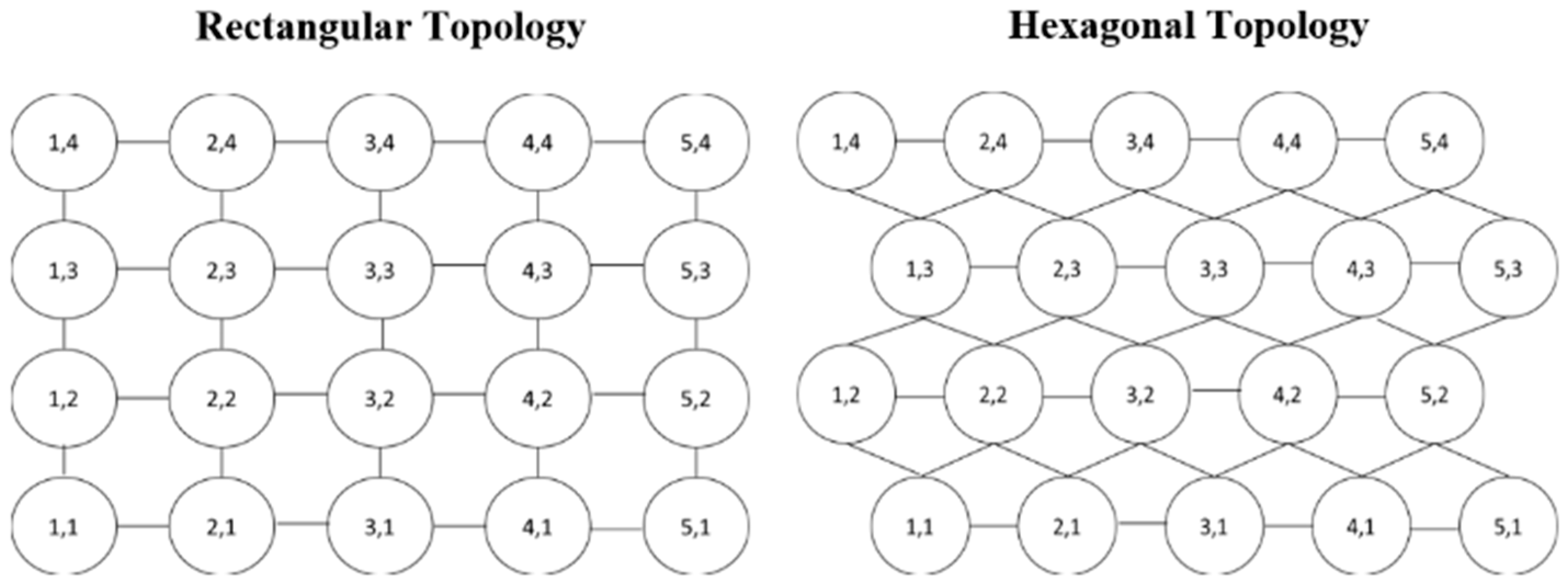
In this section, a single-layer 2D grid is utilized as the weights that are assigned according to the datasets. Generally, SOM weights could be assigned as either a rectangular or hexagonal topology, as shown in Figure 1.
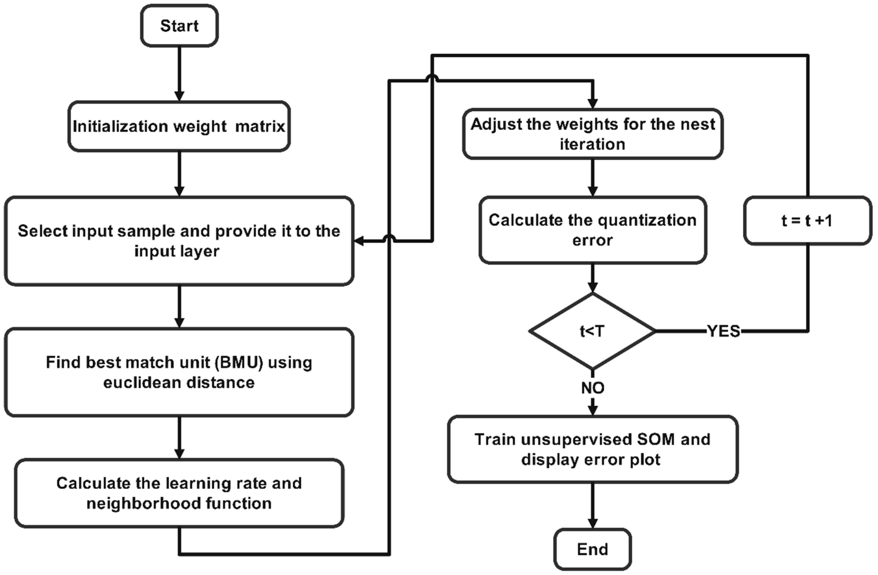
In this study, the weights were initialized in the hexagonal topology. Moreover, the number of neurons in the map is fixed and decided in advance. In practice, a reasonable number of weight maps might be chosen according to the clusters that need to be identified to prevent the weight neurons becoming widely spaced over the input dataset, resulting in a poor model distribution. In this study, random initialization of weights are used. As shown in Figure 2, after the flowchart of SOM algorithm and the weight initialization, a datapoint will be selected randomly from the dataset. Following the searching for the best matching unit (BMU) compares the Euclidean distance between the randomly selected input and all the other weights.
The weight with a shorter distance to the selected datapoint is chosen as BMU. The Euclidean distance formula is given as follows:
After finding the BMU, the learning rate, α(t), is updated, and the neighborhood function, h(t), is calculated. To calculate h(t), radius, σ(t), is supplied and the Euclidean distance, d, between the BMU and the other weight that need to be updated is calculated. Generally, this is performed for all the SOM nodes. The formulas for the learning rate, radius, the neighborhood function, and Euclidean distance are express as follows:
where σ0 chosen in this study is 5 and T is the total epoch. The weight matrix is updated using the following formula:
After updating the weight matrix, the average quantization error is calculated as follows:
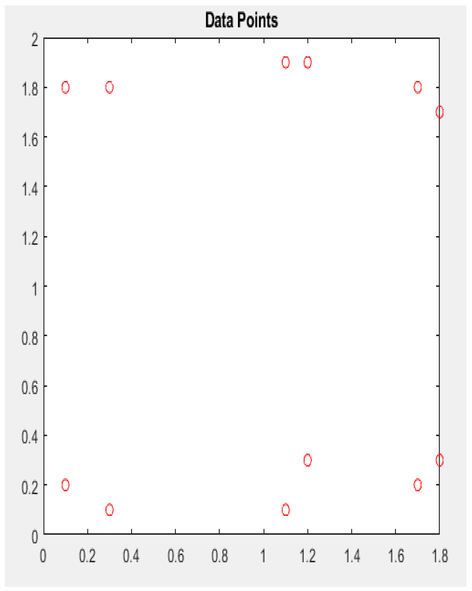
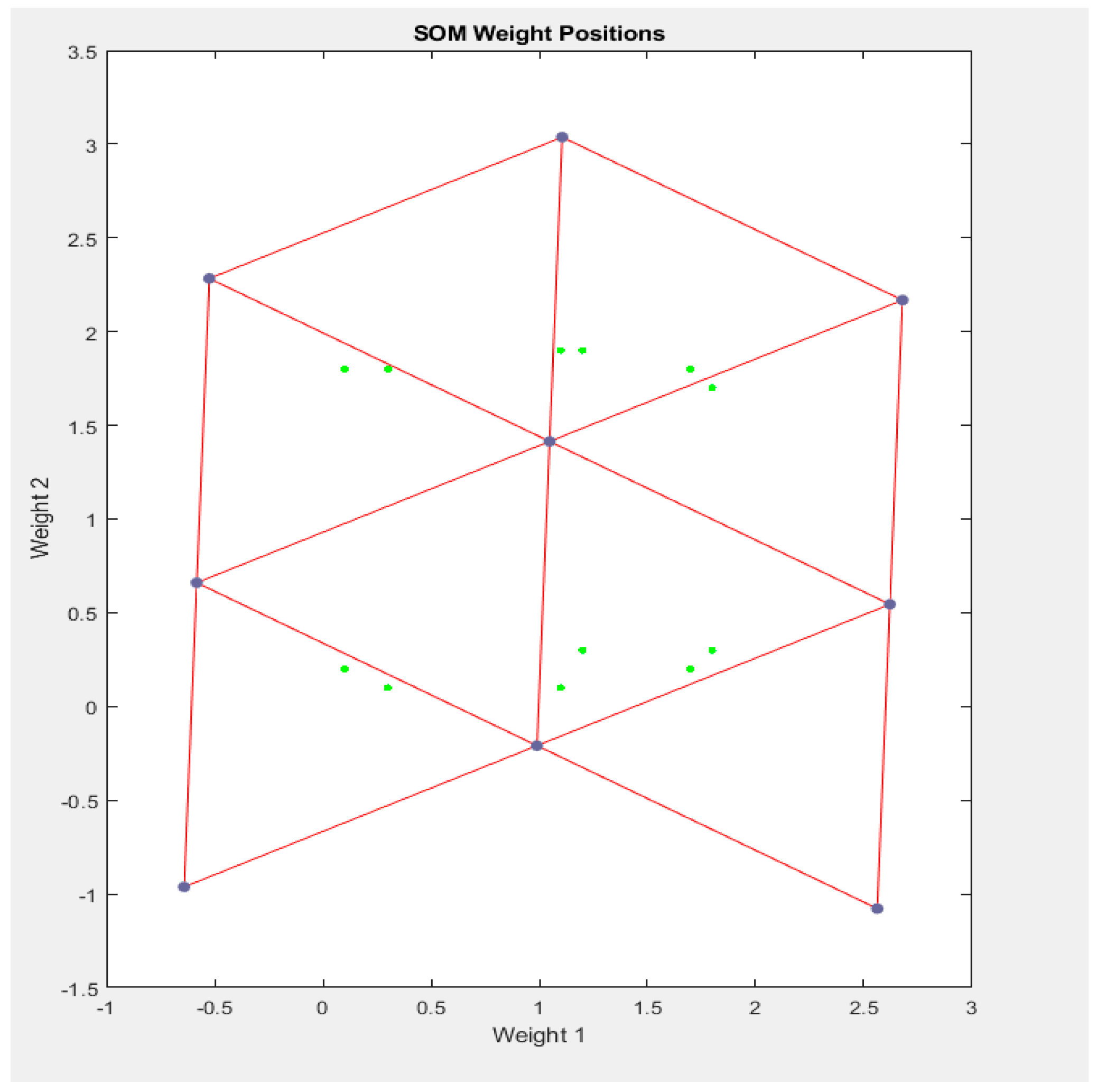
where x(t) is the input sample, BMU is the best matching unit. Hence, the average quantization error at a specific iteration can be interpreted as the average of the sum of differences between all x vectors and its best matching unit at the specific iteration. This error function is justified as it does the opposite of what the algorithm does, where the algorithm finds a BMU to update. Following the calculation of error, the next iteration is continued until reaching the stopping value T, which is the total epoch or iteration. The steps of the implementations of SOM algorithm are presented in Algorithm 1 [30]. These are the basic steps in the conventional SOM (CSOM) method. The conventional method discussed in this section is then formulated as optimal control problem. Examples of the working principle are performed in MATLAB using the Deep Learning Toolbox. A randomly generated dataset was used to portray the clustering process using SOM. Figure 3 shows that the dataset has 12 datapoints. SOM with map size of 3 by 3 was used to cluster this dataset. The result can be seen in the trained SOM column. We can observe that the 3 weights on the top and the 3 weights on the bottom are assigned to 2 datapoints each. This simply means that each weight of the SOM map is a cluster by itself, and that all the clusters were identified. In terms of our results, the easiest way to visualize self-organization map is in networks with two-dimensional (2D) input vectors and 2D weights. In the example shown, the network’s input consists of two attribute values, which are x and y, and each of which represents a position in 2D space. This network will map 2D structures in such a way that a mesh that encompasses the inputs will be generated. A simple 2D dataset along with 2D SOM weights was used to demonstrate the training of SOM.
| Algorithm 1 SOM algorithm |
| Input: A set of parameters, X = [x1, x2, …, xn]. |
| Output: set of prototype Y = [y1, y2, …, xm]. |
| 1: Initialized (Y) randomly |
| 2: repeat select x ϵ X randomly |
| 3: find y✕ such that d(x, y✕) = min{d(x, y)|y ϵ Y} |
| 4: for all y ϵ N(y✕) do |
| 5: y = y + η(x − y) |
| 6: reduce learning rate η |
| 7: until satisfy condition |
| 8: end for |
The datapoints in the 2D graph and the map initialization on the dataset are illustrated in Figure 3. However, Figure 4 shows the initialize and trained SOM model on the respective dataset. It can be observed that this network seeks to arrange the neurons such that a comparatively small distance between all neurons emerges. These experiments served as a catalyst for developing an optimal control-based Kohonen self-organizing map algorithm. This experiment was performed using the Deep Learning Toolbox in MATLAB; however, for this project, code has been written in MATLAB based on the functions on SOM toolbox.
3.2. Formulation of SOM as Optimal Control Problem
After thorough grasp on the fundamentals of optimal control by reviewing research papers on solving optimal control using Pontryagin’s Minimum Principal problem, reading the lecture notes, and understanding the overall operation of SOM, SOM has been modeled as optimal control problem in two different possible methods. As for the weight updating rule in SOM, the two most used approaches to adapt the SOM weights are the online and batch mode. Only online mode is considered in this project to use the learning rate as the control variable in the optimal control problem and the datasets used for analysis contain only two attributes. This is after understanding the fundamental way of the SOM nodes organizes themselves on the dataset to cluster. When the datapoint is selected randomly in each iteration, the best matching unit or the closest SOM node to the datapoint is affected the most during the weight updating process. The first method is modeled taking this effect into account. This is denoted as SOMOC1 throughout this study. In the first model, SOMOC1, SOM has been modeled as optimal control problem considering only the best matching unit’s weight updating equations as the state equations in the Hamiltonian equation formation. In the second model, which is denoted as SOMOC2 throughout this report, all the nodes of the SOM are considered as the state equations in the formation of Hamiltonian equation. The performance of these two proposed algorithms is evaluated on the synthetic datasets.
Generally, the Hamiltonian takes the form to solve the Pontryagin’s minimum principal problem [31,32]:
where is the objective function and is the state equation, is the state variable(s) and is the set of choice variable (s).
- (1)
- Formulation of SOMOC1 Model
The objective function of minimizing the mean quantization error is express as follows:
In formulating the SOM algorithm as the optimal control problem to minimize the objective function stated above, the state equations considered in the first model are the best matching unit’s weight updating equations. The weights of the SOM in twodimensions are represented in x and y dimensions. Both the weights are updated at the same time throughout the training period. Hence, the weight updating equations are defined as two equations, one for the x dimension and another for the y dimension. The equations are as follows:
The simplified state equation to interpret easily is as follows:
The Hamiltonian equation for the SOM as optimal control problem considering only the best matching unit’s weight updating equation as the state equations is as follows:
where x(t) denotes datapoint at time t, represent the x, y coordinates of the best match units, respectively. represent x, y, coordinates of SOM nodes with two costate. Then, the costate equations are express as follows:
The summation of means all the datapoints that select the specific best matching unit at the specific iteration as its best matching unit during the calculation of quantization error. The switching function will be as follows:
- (2)
- Formulation of SOMOC2 model
Consider SOM with the map of (N × M) dimension on the cartesian x and y plane. When the weights are represented in the format of [(N × M),2] matrix, and all the equations to update the weights of the SOM are considered as the state equations, the Hamiltonian equation will be as follows:
The costate equations will be as follows:
The switching function is as follows:
where r is all the datapoints that select the same SOM node as its best matching unit. An example of the formula formulated above is shown below. Consider SOM with the map of (2 × 2) dimension and four datapoints . The weights are represented in the format of [(2 × 2),2] matrix and all datapoints are listed in Table 2. The formulation of Hamiltonian Equation (28).
where and are best matching unit for the respective datapoint in the radical in which it is situated. The best matching unit for the respective datapoint is calculated using the Euclidean distance formula. It is written as and to represent the fact that the best matching unit is any weight between that range of weight values of the SOM, as stated in Table 3. and are the coordinates of the randomly selected datapoints in x and y dimensions, respectively. The costate equations are as follows:
In the above costate equations, to are the datapoints that have selected the specific weights that are derived with respect to the costate equation as its best matching unit. The switching function will be as follows:
4. Results and Discussion
This section describes the data collection and the experimental results. Moreover, this section benchmarks the proposed model with several datasets to justify the robustness of the proposed work. A comparison between both the proposed SOM algorithms is also presented in this section. All simulation results were conducted in MATLAB toolboxes on a 1.8 GHz Intel Core i7-8565U, with 8GB of memory, and NVIDIA GeForce MX150.
4.1. Data Collection and Preparation
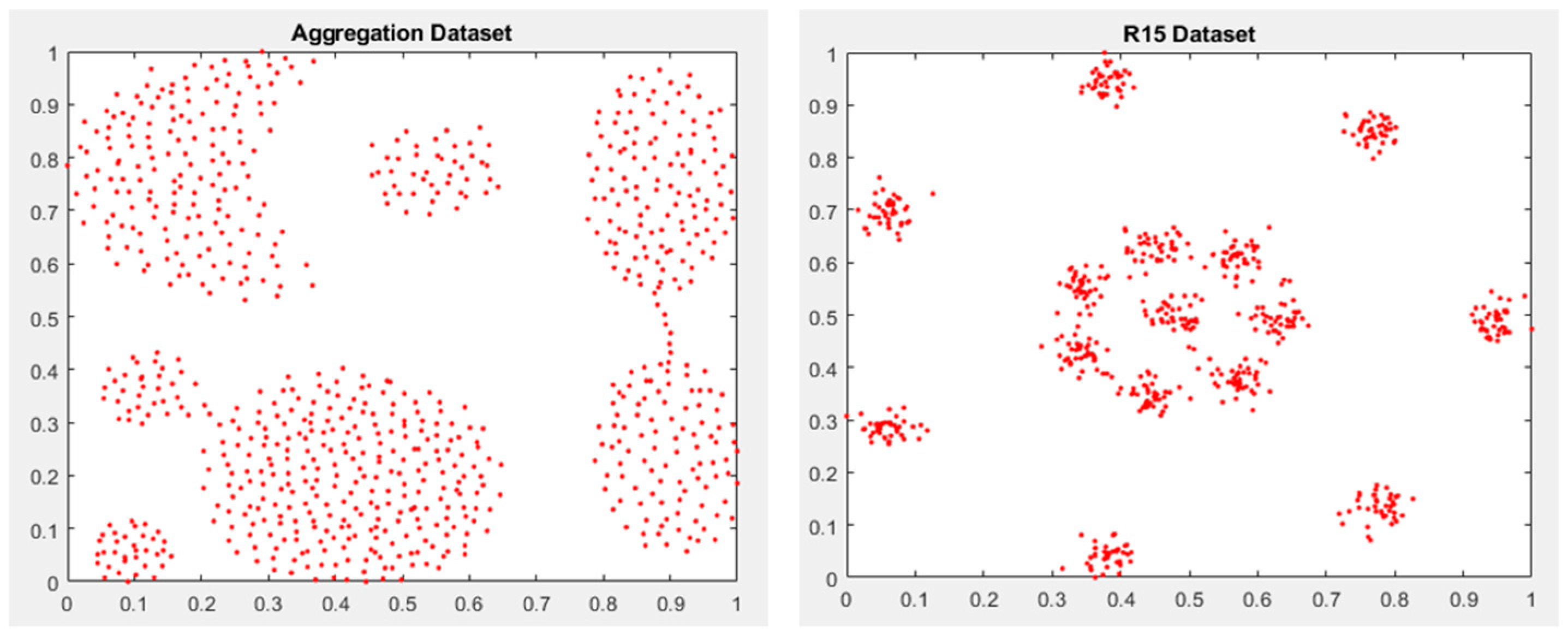
In this work, two datasets are utilized, namely, the aggregation dataset and the R15 dataset. The datasets are obtained from UCI machine learning repository as shown in Figure 5.
Normalization is a process in database design that is used to reduce data redundancy and improve data integrity by organizing data into separate tables based on their relationships. This way, data are stored in a more efficient and consistent manner, reducing the risk of data duplication. Furthermore, normalization datasets are essential when attributes are dealt with at a different scale; otherwise, it can dilute the efficacy of an equally essential attribute (on the lower scale), since other attributes have bigger values. In other words, when dealing with multiple attributes that have values on various scales, this may lead to bad data models. The purpose of normalization is to ensure that every datapoint has the same scale, ensuring that each characteristic is equally meaningful. One of the most prevalent methods of data normalizing is min–max normalization. The minimum value of each feature is converted to a 0, the highest value is converted to a 1, and all other values are converted to a decimal between 0 and 1. One notable drawback of min–max normalization is that it does not handle outliers well. The formula for min–max normalization is given as follows [33]:
The normalized values will be closer to 0 if the unnormalized data have a significant standard deviation. In this work, a min-max normalization method was employed because the synthetic datasets used to evaluate the performance of SOMOC1 and SOMOC2 do not contain any outliers. Furthermore, all the synthetic datasets used in this study are related to clustering algorithms. Mainly, the nodes of the SOM were normalized as well.
4.2. Comparing the Performance of the Proposed Algorithms
A comparison was performed using both the algorithms SOMOC1 and SOMOC2 by comparing with the conventional SOM method. The map size to be used on the dataset was obtained based on the heuristic SOM initializing formula proposed in [34]. The formula utilized to determine the nodes is given as follows:
where M is the number of neurons, which is an integer close to the result of the right-hand side of the equation, and N is the number of datapoints. The datasets used in this section are named aggregation and R15. The samples chosen randomly throughout the epochs were kept identical in the three algorithms when run on each dataset for comparison.
- (1)
- Experiment Results Based on Aggregation Dataset
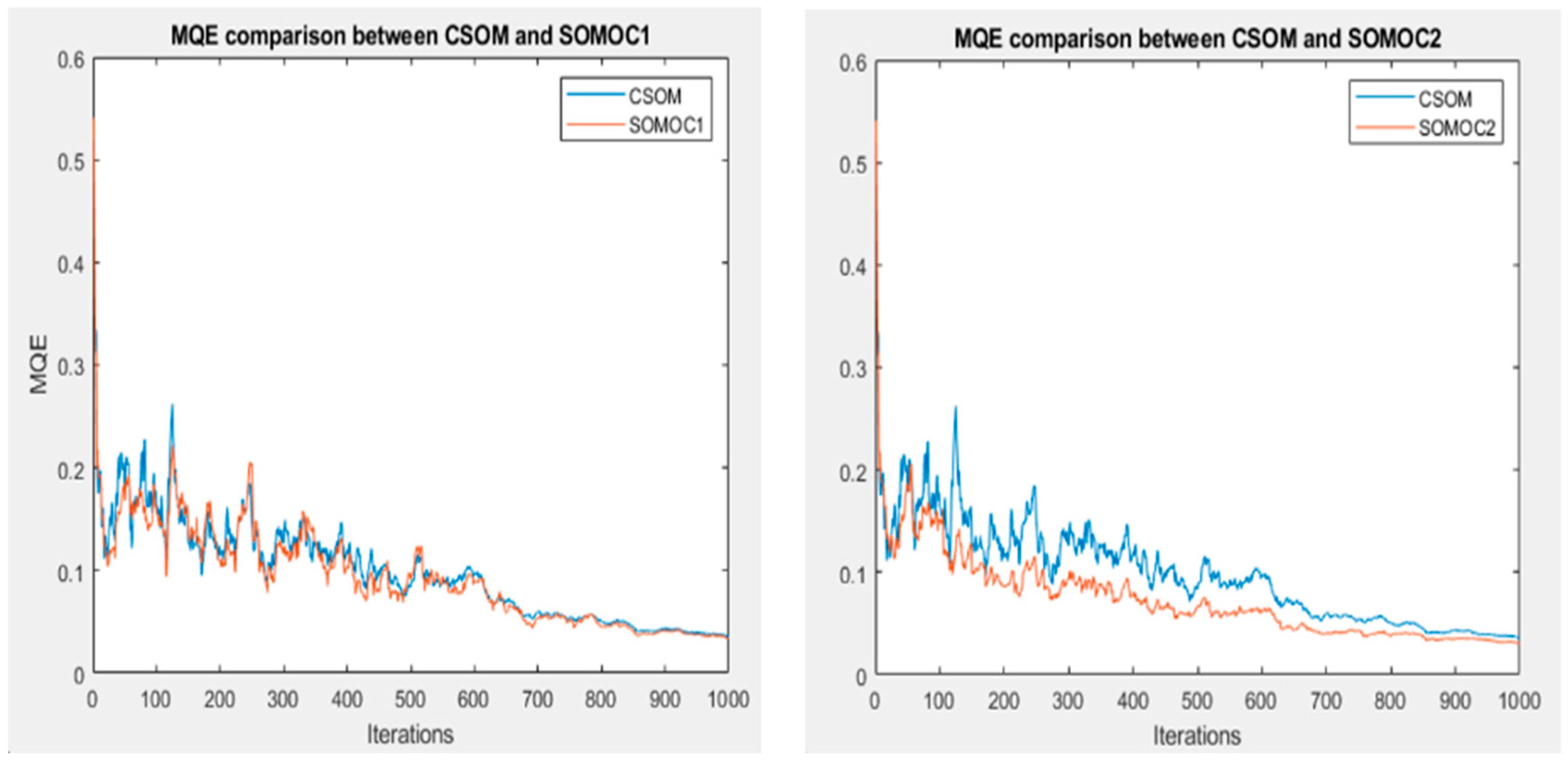
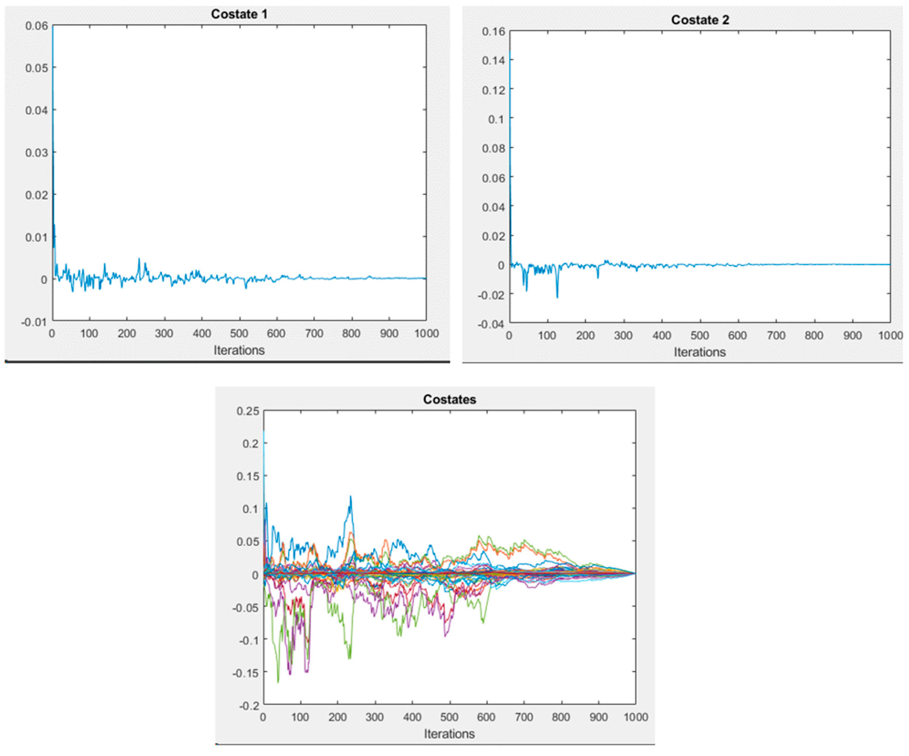
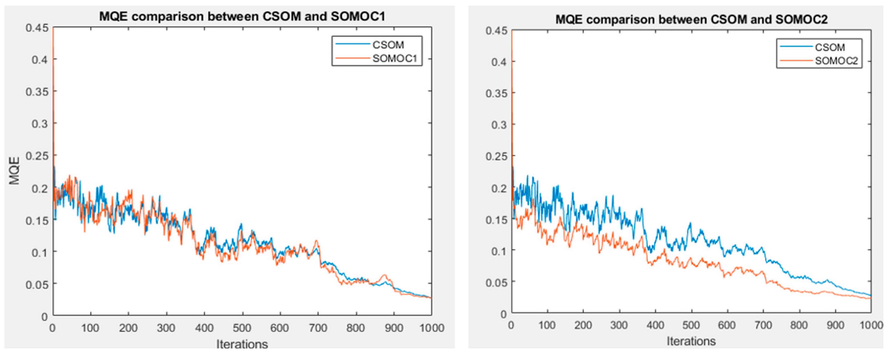
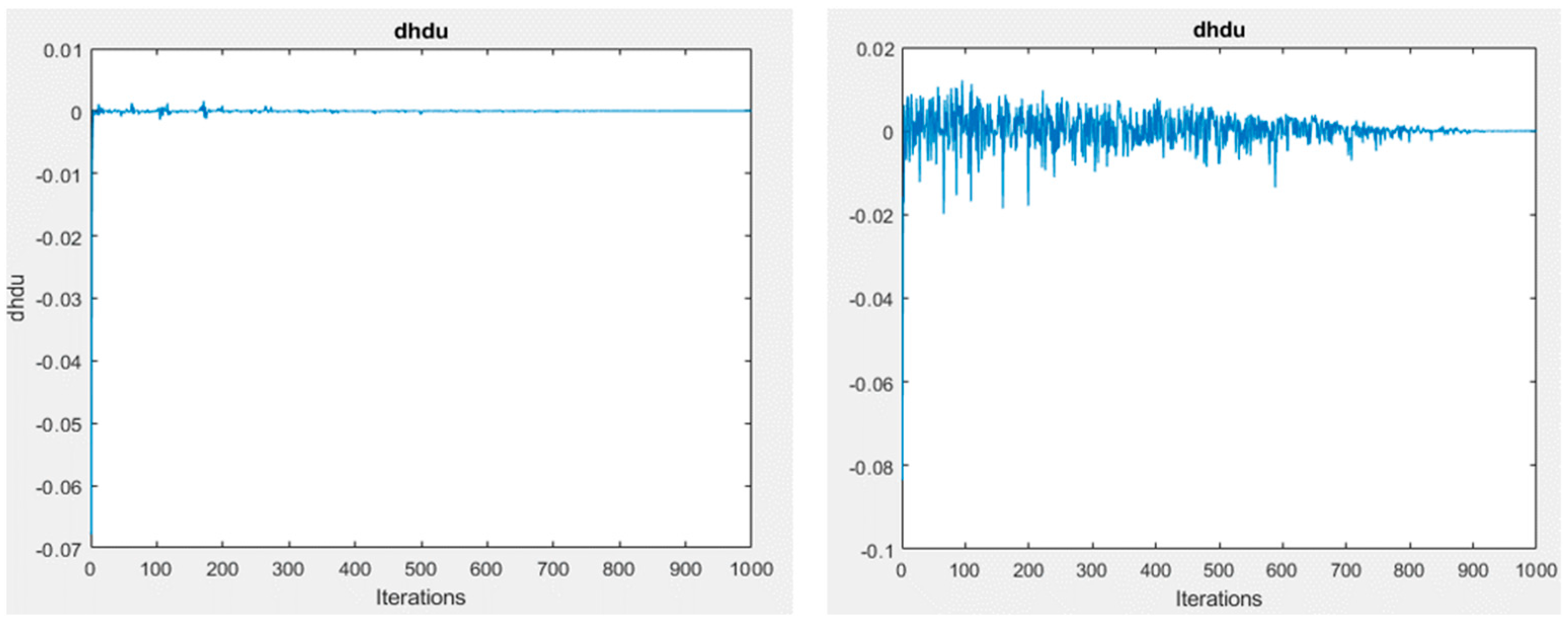
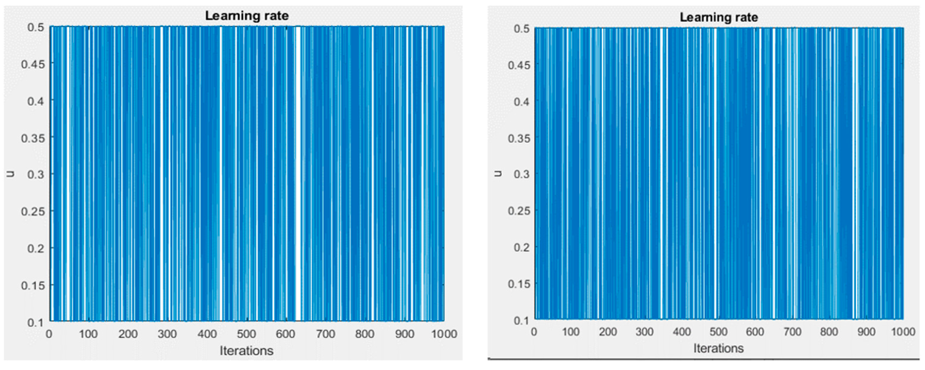
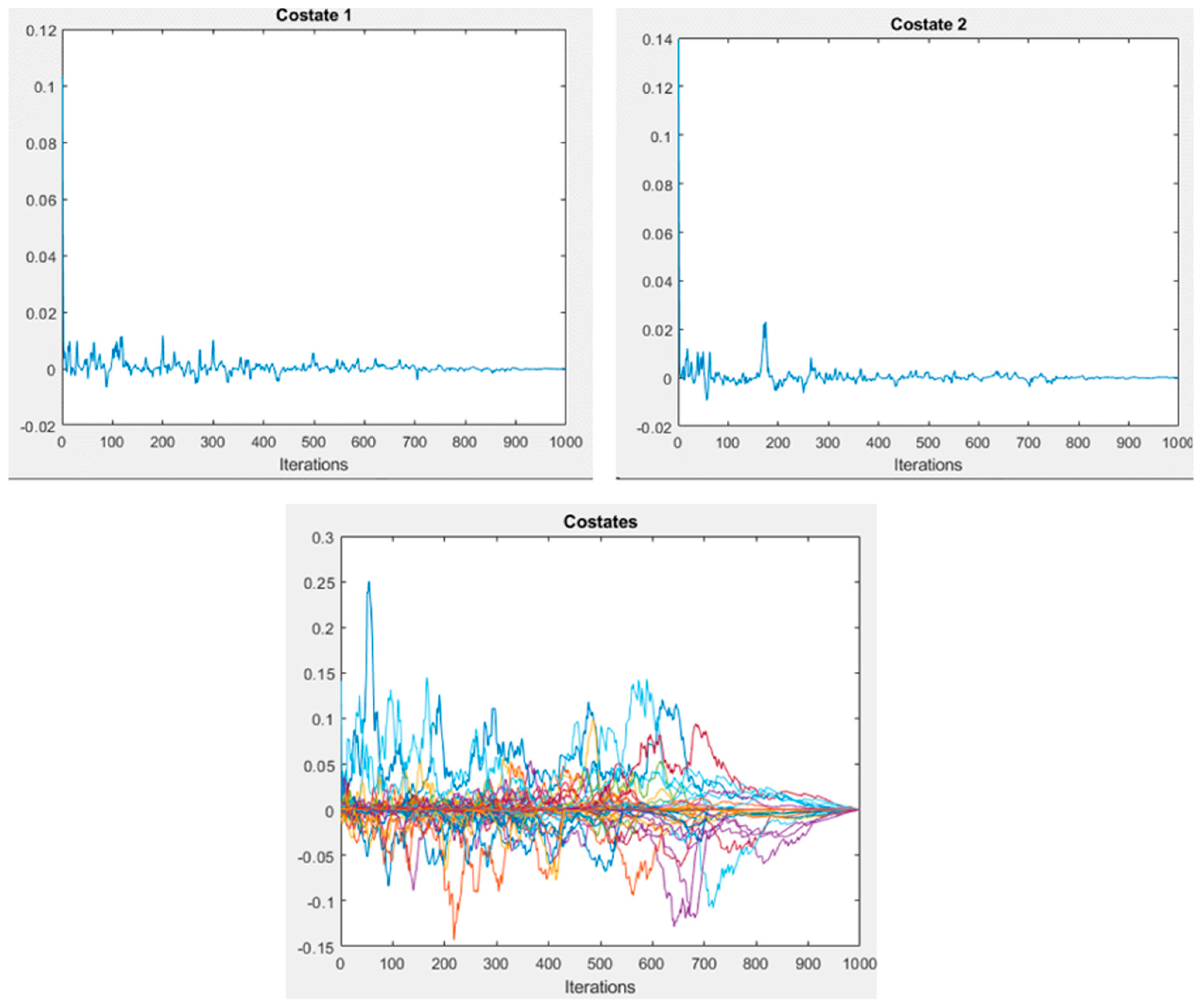
The map size chosen for this dataset is 12 × 12 with 1000 iterations. The formulated equations of the SOMOC1 and SOMOC2 algorithms are discussed in Section 3.2. SOMOC1 has T values of 788 and on the other hand, the SOMOC2 algorithm has 788, 12, and 12 for T, N, and M, respectively. The values for the costates were found using the ODE45 function in MATLAB, and those values are used to find the values of the switching function. Based on the values of the switching function, the minimum and maximum learning rate, or the control variable were supplied to the training algorithms. The comparison quantization errors of CSOM, SOMOC1, and SOMOC2 based on the aggregation dataset are illustrated in Figure 6 and the switch functions, control variables, and costates are shown in Figure 7, Figure 8 and Figure 9, respectively. Figure 9 shows the costate variable of SOMOC1 and SOMOC2 based on aggregation dataset, it can be observed that costate of SOMOC2 includes all possible values of costate which is represented in different color
- (2)
- Experiment results based on R15 Dataset
The map size chosen for this dataset is 11 × 11 with 1000 iterations. The formulated equations of the SOMOC1 and SOMOC2 algorithms are discussed in Section 3.2. Moreover, SOMOC1 has T values of 600 and on the other hand, the SOMOC2 algorithm has 600, 11, and 11 for T, N, and M, respectively. The values for the costates were found using the ODE45 function in MATLAB, and those values are used to find the values of the switching function. Based on the values of the switching function, minimum and maximum learning rate, or the control variable were supplied to the training algorithms. The comparison quantization errors of CSOM, SOMOC1, and SOMOC2 based on an aggregation dataset are illustrated in Figure 10, and the switch functions, control variables, and costates are shown in Figure 11, Figure 12 and Figure 13, respectively. Figure 13 shows the costate variable of SOMOC1 and SOMOC2 based on R15 dataset, it can be observed that costate of SOMOC2 includes all possible costate values which is represented in different color.
The comparison performance of The comparison performance of the average results from 10 runs are demonstrated in Table 4. SOMOC1 shows an improvement of 4.34% over CSOM on the aggregation dataset and a 3.61% improvement on dataset R15 in terms of the final average quantization error. SOMOC2 shows an improvement of 14.35% over CSOM on the aggregation dataset and a 22.36% improvement over CSOM in dataset R15 in terms of the final objective function value. The time taken to complete the training does not show a significant improvement in both the proposed algorithms, but SOMOC2 managed to reach the saturation point of the mean quantization error earlier than CSOM.
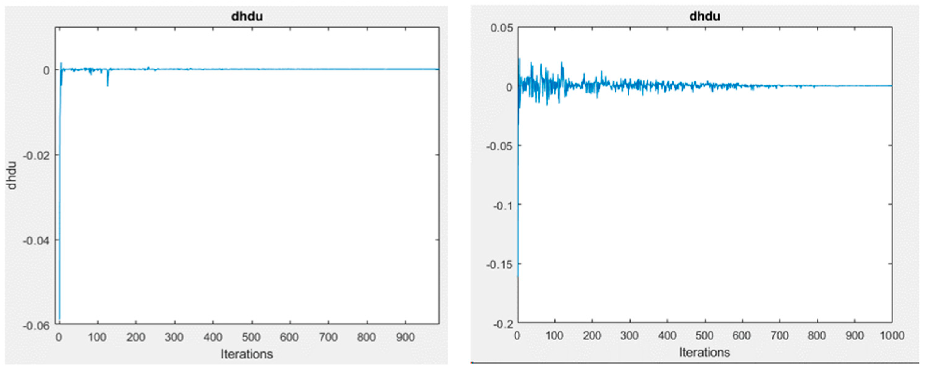
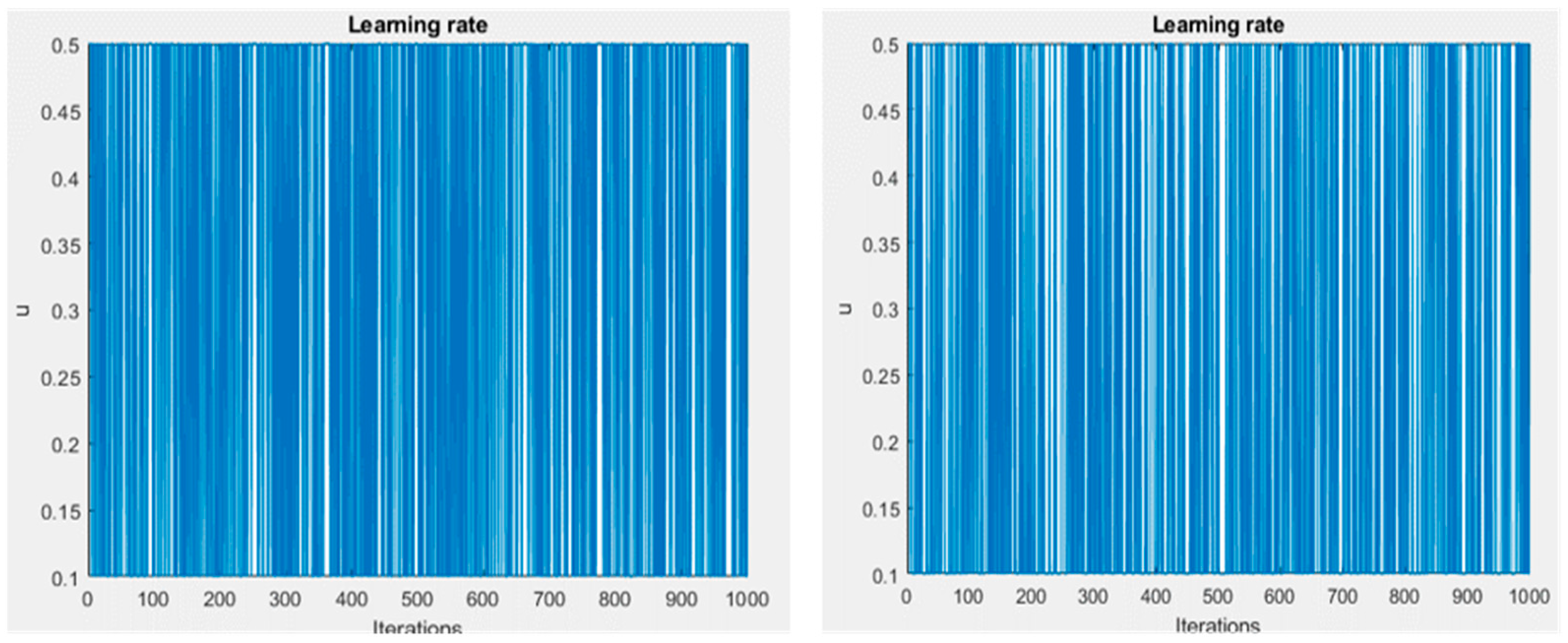
However, it can be seen from results that produced by the proposed algorithms, it has is a fluctuation at the beginning of the training that approaches the value of 0 as the training progresses. The value of fluctuates right above and below 0 as the training progresses and causes the applied bang-bang control method to frequently choose the minimum and maximum learning rate value during the training. This can be seen in the plots of the learning rates or the control variable shown for all the cases above.
Furthermore, in the case of SOMOC2 algorithm, reaches a value with a fifth decimal place or a very small value as the training progresses. This simply means that it is in the singular arc period. The reason for the to fluctuate in the first place is due to the derivative of the objective function. The objective function in the Hamiltonian equation is the mean quantization error that produces a positive value. The mean quantization error is the average of the absolute difference value of all the datapoints and its best matching unit present in a dataset. When it is differentiated against the weight of the SOM, either the weight in the x or y dimension to obtain the adjoint equations, the costates are highly impacted by this differentiation. What happens here is that, when differentiated against the respective weight in the x or y dimension to obtain the adjoint equation, the numerator will contain the difference between either the x or y coordinate of the datapoint and the weight. The numerator can now be either positive or negative. Hence, the values differ so much at the beginning of training. This value impacts the costate values and subsequently leads to high fluctuations in the early part of . However, this is the marginal cost that is obtained to minimize the constraints imposed by the state equation. This is justified as the SOMOC1 and SOMOC2 models choose the highest learning rate at the beginning of the training as the switching function values are negative. The fluctuation is expected to be obtained to minimize the objective function. However, the switching function enters the singular arc period as the training progresses. The possible solutions to address this problem are through finding an equation for the learning rate when it enters the singular arc period. To obtain the value of the learning rate during the singular arc, the formulated of the Hamiltonian equations for SOMOC1 and SOMOC2, the switching function, and , are differentiated against time, . However, the formula for the learning rate could not be formulated, as it vanishes during the derivation. This leads to an infinite order singular arc problem. Possible solutions to this problem are suggested in the next section. Moreover, to show the impact of the clustering, two random orders have been chosen to compare with benchmark datasets in terms of the average error and time consumed, as shown in Table 4 and Table 5, respectively. Furthermore, the comparisons of CSOM, SOMOC1, and SOMOC2 of random average 10 runs are listed in Table 6.
5. Conclusions and Future Study
In this work, the conventional SOM, which utilizes the online mode weight updating equation, has been modeled as an optimal control problem, which has been formulated as a Hamiltonian equation while considering the online mode weight updating equation as the state equation and the mean quantization error as the objective function. Furthermore, two models have been proposed in this work: the first model is SOMOC1, which formulates the Hamiltonian equation in such a way that the weights are represented in the x and y dimensions of the best matching unit that is considered in the state equation. However, the reason to consider only the best matching unit is to target the certain cluster identified by the best matching unit and minimize the error. The second model is SOMOC2, in which all the SOM nodes are considered as the state equations in the formulation of the Hamiltonian equation. SOMOC2 provides better results compared to the conventional SOM because the algorithms now have the option to choose between the control variable, which is the learning rate depending on the switching function that is influenced by the costates and aims to minimize the objective function by relaxing the state equations. The state equations represent the constraints of the minimization problem, and the costate variables represent the marginal cost of violating those constraints. Since the SOMOC2 model comprises all the weights of the SOM in the Hamiltonian equation, it tends to provide better results compared to the SOMOC1 model. Despite SOMOC2 choosing all the node weights, it shows marginally less computational time compared to SOMOC1. In SOMOC1, which works with the best matching unit (BMU) node, the sorting process is carried out to search for the BMU weight. The empirical results demonstrate that the SOMOC2 algorithm shows a better performance than the SOMOC1 algorithm. Generally, SOMOC2 provides a 15% better improvement in terms of the error compared to CSOM. In the future, more complex and larger datasets should be used in our developed models to verify the application of SOMOC1 and 2 to larger dataset problems. Further study could be achieved to find an equation or a proper learning rate that is appropriate to be applied to the singular arc period, and with this, the training of SOM could be more adaptive in such a way to minimize the quantization error.
Author Contributions
Conceptualization, A.N.A. and J.K.; Data curation, I.A.B., M.H., M.A.A.B. and N.A.A.; Formal analysis, I.A.B., S.K., M.H. and M.A.A.B.; Funding acquisition, I.A.B. and S.K.; Investigation, A.N.A. and J.K.; Methodology, A.N.A., J.K. and I.A.B.; Resources, M.A.A.B. and N.A.A.; Software, S.K., M.H., M.A.A.B. and N.A.A.; Validation, S.K., M.H. and N.A.A.; Writing—original draft, J.K.; Writing—review and editing, A.N.A. and I.A.B. All authors have read and agreed to the published version of the manuscript.
Funding
This work was supported by the Malaysian Ministry of Higher Education through the Fundamental Research Grant Scheme under Grant FRGS/1/2020/ICT02/UM/02/2. Also, the work is supported by Deanship of Scientific Research at King Khalid under grant number (RGP.1/74/43).
Data Availability Statement
Not applicable.
Acknowledgments
The authors would like to extend their sincere appreciation to the Malaysian Ministry of Higher Education through the Fundamental Research Grant Scheme under Grant FRGS/1/2020/ICT02/UM/02/2. The authors extend their appreciation to the Deanship of Scientific Research at King Khalid University for funding this work through the Small Groups Project under grant number (RGP.1/74/43).
Conflicts of Interest
The authors declare no conflict of interest.
References
- Soon, F.C.; Khaw, H.Y.; Chuah, J.H.; Kanesan, J. Vehicle logo recognition using whitening transformation and deep learning. Signal Image Video Process. 2018, 13, 111–119. [Google Scholar] [CrossRef]
- Vesanto, J.; Alhoniemi, E. Clustering of the self-organizing map. IEEE Trans. Neural Netw. 2000, 11, 586–600. [Google Scholar] [CrossRef] [PubMed]
- Kohonen, T. The self-organizing map. Proc. IEEE 1990, 78, 1464–1480. [Google Scholar] [CrossRef]
- Wehrens, H. Data mapping: Linear methods versus nonlinear techniques. Compr. Chemom. 2009, 2, 619–633. [Google Scholar]
- Sun, Y. On quantization error of self-organizing map network. Neurocomputing 2000, 34, 169–193. [Google Scholar] [CrossRef]
- Widiyaningtyas, T.; Zaeni, I.A.E.; Wahyuningrum, P.Y. Self-Organizing Map (SOM) For Diagnosis Coronary Heart Disease. In Proceedings of the 2019 4th International Conference on Information Technology, Information Systems and Electrical Engineering (ICITISEE), Yogyakarta, Indonesia, 20–21 November 2019; pp. 286–289. [Google Scholar]
- Wankhede, S.B. Study of back-propagation and self organizing maps for robotic motion control: A survey. In Proceedings of the 2017 International Conference on Trends in Electronics and Informatics (ICEI), Tirunelveli, India, 11–12 May 2017; pp. 537–540. [Google Scholar]
- Ristic, D.M.; Pavlovic, M.; Reljin, I. Image segmentation method based on self-organizing maps and K-means algorithm. In Proceedings of the 2008 9th Symposium on Neural Network Applications in Electrical Engineering, Belgrade, Serbia, 25–27 September 2008; pp. 27–30. [Google Scholar]
- Zhang, X.-Y.; Chen, J.-S.; Dong, J.-K. Color clustering using self-organizing maps. In Proceedings of the 2007 International Conference on Wavelet Analysis and Pattern Recognition, Beijing, China, 2–4 November 2007; pp. 986–989. [Google Scholar]
- Soon, F.C.; Khaw, H.Y.; Chuah, J.H.; Kanesan, J. Semisupervised PCA convolutional network for vehicle type classification. IEEE Trans. Veh. Technol. 2020, 69, 8267–8277. [Google Scholar] [CrossRef]
- Chong, E.K.; Zak, S.H. An Introduction to Optimization; John Wiley & Sons: Hoboken, NJ, USA, 2013; Volume 75. [Google Scholar]
- Zain, M.Z.B.M.; Kanesan, J.; Kendall, G.; Chuah, J.H. Optimization of fed-batch fermentation processes using the Backtracking Search Algorithm. Expert Syst. Appl. 2018, 91, 286–297. [Google Scholar] [CrossRef]
- Eswaran, U.; Ramiah, H.; Kanesan, J. Power amplifier design methodologies for next generation wireless communications. IETE Technol. Rev. 2014, 31, 241–248. [Google Scholar] [CrossRef]
- Badruddin, I.A.; Hussain, M.K.; Ahmed, N.S.; Kanesan, J.; Mallick, Z. Noise characteristics of grass-trimming machine engines and their effect on operators. Noise Health 2009, 11, 98–102. [Google Scholar] [CrossRef]
- Jeevan, K.; Quadir, G.; Seetharamu, K.; Azid, I. Thermal management of multi-chip module and printed circuit board using FEM and genetic algorithms. Microelectron. Int. 2005, 22, 3–15. [Google Scholar] [CrossRef]
- Hoo, C.-S.; Jeevan, K.; Ganapathy, V.; Ramiah, H. Variable-Order ant system for VLSI multiobjective floorplanning. Appl. Soft Comput. 2013, 13, 3285–3297. [Google Scholar] [CrossRef]
- Hoo, C.-S.; Yeo, H.-C.; Jeevan, K.; Ganapathy, V.; Ramiah, H.; Badruddin, I.A. Hierarchical congregated ant system for bottom-up VLSI placements. Eng. Appl. Artif. Intell. 2013, 26, 584–602. [Google Scholar] [CrossRef]
- Tavoosi, J.; Suratgar, A.A.; Menhaj, M.B.; Mosavi, A.; Mohammadzadeh, A.; Ranjbar, E. Modeling renewable energy systems by a self-evolving nonlinear consequent part recurrent type-2 fuzzy system for power prediction. Sustainability 2021, 13, 3301. [Google Scholar] [CrossRef]
- Hofmann, S.; Borzì, A. A sequential quadratic hamiltonian algorithm for training explicit RK neural networks. J. Comput. Appl. Math. 2022, 405, 113943. [Google Scholar] [CrossRef]
- Breitenbach, T.; Borzì, A. A sequential quadratic Hamiltonian scheme for solving non-smooth quantum control problems with sparsity. J. Comput. Appl. Math. 2020, 369, 112583. [Google Scholar] [CrossRef]
- Alkawaz, A.N.; Abdellatif, A.; Kanesan, J.; Khairuddin, A.S.M.; Gheni, H.M. Day-Ahead Electricity Price Forecasting Based on Hybrid Regression Model. IEEE Access 2022, 10, 108021–108033. [Google Scholar] [CrossRef]
- Min, E.; Guo, X.; Liu, Q.; Zhang, G.; Cui, J.; Long, J. A survey of clustering with deep learning: From the perspective of network architecture. IEEE Access 2018, 6, 39501–39514. [Google Scholar] [CrossRef]
- Lasri, R. Clustering and classification using a self-organizing MAP: The main flaw and the improvement perspectives. In Proceedings of the 2016 SAI Computing Conference (SAI), London, UK, 13–15 July 2016; pp. 1315–1318. [Google Scholar]
- Vesanto, J.; Himberg, J.; Alhoniemi, E.; Parhankangas, J. Self-organizing map in Matlab: The SOM Toolbox. In Proceedings of the Matlab DSP Conference, Espoo, Finland, 16–17 November 1999; pp. 16–17. [Google Scholar]
- MathWorks. Plotsomhits. 2022. Available online: https://www.mathworks.com/help/deeplearning/ref/plotsomhits.html (accessed on 1 November 2022).
- Ferguson, B.S.; Lim, G.C.; Lim, G.C. Introduction to Dynamic Economic Models; Manchester University Press: Manchester, UK, 1998. [Google Scholar]
- Alkawaz, A.N.; Kanesan, J.; Khairuddin, A.S.M.; Chow, C.O.; Singh, M. Intelligent Charging Control of Power Aggregator for Electric Vehicles Using Optimal Control. Adv. Electr. Comput. Eng. 2021, 21, 21–30. [Google Scholar] [CrossRef]
- Kirk, D.E. Optimal Control Theory: An Introduction; Courier Corporation: North Chelmsford, MA, USA, 2004. [Google Scholar]
- Macki, J.; Strauss, A. Introduction to Optimal Control Theory; Springer Science & Business Media: Berlin/Heidelberg, Germany, 2012. [Google Scholar]
- Günter, S.; Bunke, H. Self-organizing map for clustering in the graph domain. Pattern Recognit. Lett. 2002, 23, 405–417. [Google Scholar] [CrossRef]
- Casas, E. Pontryagin’s principle for state-constrained boundary control problems of semilinear parabolic equations. SIAM J. Control. Optim. 1997, 35, 1297–1327. [Google Scholar] [CrossRef]
- Serrao, L.; Onori, S.; Rizzoni, G. ECMS as a realization of Pontryagin’s minimum principle for HEV control. In Proceedings of the 2009 American Control Conference, St. Louis, MO, USA, 10–12 June 2009; pp. 3964–3969. [Google Scholar]
- Ramakrishna, S.S.; Anuradha, T. AN EFFECTIVE FRAMEWORK FOR DATA CLUSTERING USING IMPROVED K-MEANS APPROACH. Int. J. Adv. Res. Comput. Sci. 2018, 9, 516–520. [Google Scholar] [CrossRef]
- Gorgoglione, A.; Castro, A.; Gioia, A.; Iacobellis, V. Application of the Self-organizing Map (SOM) to Characterize Nutrient Urban Runoff. In Proceedings of the International Conference on Computational Science and Its Applications, Cagliari, Italy, 1–4 July 2020; pp. 680–692. [Google Scholar]
Figure 1.
Structure of two topologies.

Figure 2.
Flowchart of the SOM algorithm.

Figure 3.
Random data.

Figure 4.
Initialized and trained SOM model on the respective dataset.

Figure 5.
Left: aggregation dataset, right: R15 dataset.

Figure 6.
Comparison of quantization errors obtained from SOMOC1 and SOMOC2.

Figure 7.
Switching function: left: SOMOC1, right: SOMOC2.

Figure 8.
Control variable: left: SOMOC1, right: SOMOC2.

Figure 9.
Costate 1 and 2 of SOMOC1 and costate of SOMOC2 based on an aggregation dataset.

Figure 10.
Figure 2: Comparison of quantization errors obtained from SOMOC1 and SOMOC2.
Figure 10.
Figure 2: Comparison of quantization errors obtained from SOMOC1 and SOMOC2.

Figure 11.
Figure 3: Switching function: left: SOMOC1, right: SOMOC2.
Figure 11.
Figure 3: Switching function: left: SOMOC1, right: SOMOC2.

Figure 12.
Learning rate (control signal variable) of SOMOC1 and SOMOC2.

Figure 13.
Costate 1 and 2 of SOMOC1 and costate of SOMOC2 based on an R15 dataset.


Table 1.
The symbols and definition used in this study.
| Symbol | Definition |
|---|---|
| Datapoint at time t | |
| x—coordinate of the randomly chosen datapoint | |
| y—coordinate of the randomly chosen datapoint | |
| Neighborhood function at time t | |
| /u(t) | Learning rate at time t/control at time t |
| Total number of datapoints | |
| x—coordinate of the best matching unit | |
| y—coordinate of the best matching unit | |
| x—coordinate of the SOM node | |
| y—coordinate of the SOM node |
Table 2.
The datapoints and its representation.
| Datapoints | Coordinates | |
|---|---|---|
| x | y | |
Table 3.
The SOM weights and its representation.
| Weights | Coordinates | |
|---|---|---|
| x | y | |
Table 4.
Comparison between CSOM, SOMOC1, and SOMOC2 averaged over 10 runs.
| Datasets | Aggregation | R15 | ||||
|---|---|---|---|---|---|---|
| SOM Algorithms | CSOM | SOMOC1 | SOMOC2 | CSOM | SOMOC1 | SOMOC2 |
| Average MQE | 0.095711 | 0.091741 | 0.070850 | 0.113570 | 0.105027 | 0.080154 |
| Final MQE | 0.036482 | 0.034899 | 0.031247 | 0.028119 | 0.027102 | 0.021832 |
| Time taken | 1.144511 | 1.154533 | 1.143495 | 1.019185 | 1.027379 | 1.018741 |
Table 5.
Comparison between CSOM, SOMOC1, and SOMOC2 averaged over 10 runs for randomized order 1.
| Datasets | Aggregation | R15 | ||||
|---|---|---|---|---|---|---|
| SOM Algorithms | CSOM | SOMOC1 | SOMOC2 | CSOM | SOMOC1 | SOMOC2 |
| Average MQE | 0.093245 | 0.092671 | 0.072342 | 0.113570 | 0.111584 | 0.078735 |
| Final MQE | 0.034212 | 0.032389 | 0.030489 | 0.027543 | 0.027099 | 0.023288 |
| Time taken | 1.156281 | 1.144356 | 1.153432 | 1.023321 | 1.026871 | 1.018232 |
Table 6.
Comparison between CSOM, SOMOC1, and SOMOC2 averaged over 10 runs for randomized order 2.
| Datasets | Aggregation | R15 | ||||
|---|---|---|---|---|---|---|
| SOM Algorithms | CSOM | SOMOC1 | SOMOC2 | CSOM | SOMOC1 | SOMOC2 |
| Average MQE | 0.095711 | 0.091741 | 0.0718230 | 0.113570 | 0.105027 | 0.079632 |
| Final MQE | 0.036482 | 0.034899 | 0.0310971 | 0.027234 | 0.026995 | 0.022842 |
| Time taken | 1.139519 | 1.154576 | 1.146389 | 1.019185 | 1.027379 | 1.019732 |
Disclaimer/Publisher’s Note: The statements, opinions and data contained in all publications are solely those of the individual author(s) and contributor(s) and not of MDPI and/or the editor(s). MDPI and/or the editor(s) disclaim responsibility for any injury to people or property resulting from any ideas, methods, instructions or products referred to in the content. |
© 2023 by the authors. Licensee MDPI, Basel, Switzerland. This article is an open access article distributed under the terms and conditions of the Creative Commons Attribution (CC BY) license (https://creativecommons.org/licenses/by/4.0/).
Share and Cite
MDPI and ACS Style
Alkawaz, A.N.; Kanesan, J.; Badruddin, I.A.; Kamangar, S.; Hussien, M.; Ali Baig, M.A.; Ahammad, N.A. Adaptive Self-Organizing Map Using Optimal Control. Mathematics 2023, 11, 1995. https://doi.org/10.3390/math11091995
AMA Style
Alkawaz AN, Kanesan J, Badruddin IA, Kamangar S, Hussien M, Ali Baig MA, Ahammad NA. Adaptive Self-Organizing Map Using Optimal Control. Mathematics. 2023; 11(9):1995. https://doi.org/10.3390/math11091995
Chicago/Turabian StyleAlkawaz, Ali Najem, Jeevan Kanesan, Irfan Anjum Badruddin, Sarfaraz Kamangar, Mohamed Hussien, Maughal Ahmed Ali Baig, and N. Ameer Ahammad. 2023. "Adaptive Self-Organizing Map Using Optimal Control" Mathematics 11, no. 9: 1995. https://doi.org/10.3390/math11091995
Note that from the first issue of 2016, this journal uses article numbers instead of page numbers. See further details here.