
Dry Friction Analysis in Doped Surface by Network Simulation Method

1
Department of Thermal and Fluid Engineering, Faculty of Industrial Engineering, Politechnic University of Cartagena, 30202 Cartagena, Spain
2
Department of Mathematics, Faculty of Mathematics, University of Murcia, 30100 Murcia, Spain
3
Department of Mechanical Engineering, Materials and Manufacturing, Faculty of Industrial Engineering, Politechnic University of Cartagena, 30202 Cartagena, Spain
4
Department of Automation, Electrical Engineering and Electronic Technology, Faculty of Industrial Engineering, Politechnic University of Cartagena, 30202 Cartagena, Spain
*
Author to whom correspondence should be addressed.
†
These authors contributed equally to this work.
Mathematics 2023, 11(6), 1341; https://doi.org/10.3390/math11061341
Submission received: 10 January 2023
/
Revised: 1 March 2023
/
Accepted: 6 March 2023
/
Published: 9 March 2023
(This article belongs to the Special Issue Theory and Application of Dynamical Systems in Mechanics)
Abstract
:Dry friction cannot be understood on a macroscopic scale without knowing what happens at the contact of sliding surfaces on an atomic scale. Tests on this scale are very expensive and very sensitive to the effects of contamination or inaccurate fittings. On the other hand, the sample dimensions are small because of the requirements of the test equipment, which makes it difficult to generalise the conclusions drawn. This work reviews the models used to analyse friction processes, and proposes the application of one of the models, the Frenkel–Kontorova–Tomlinson (FKT) model, to study the dry frictional behaviour of doped surfaces. The study shows that for concreted types of doped pattern, the behaviour can change from chaotic to periodic depending on the stiffness, which in turn are associated with temperature.
1. Introduction
Understanding friction at nanoscale is crucial for the design of mechanisms in this scale. In this way, it seems possible to deduce from the tests performed that Amontons’ and Coulomb’s laws of friction seem to work at the macroscopic scale. At the moment, it is very difficult to predict the frictional properties of a given contact, although the optimisation of these properties on surfaces of specific use is gaining importance due to the miniaturisation of mechanical systems [1,2,3,4,5,6,7,8,9,10,11,12,13] in nanotechnology.
The simplest model to interpret the experimental results related to dry friction is the Prandtl–Tomlinson (PT) model, based on the work of Prandtl [14] and Tomlinson [15]. This model consists of a point mass dragged on a surface, considered to be a reference of the relative motion, interacting elastically with a point belonging to the surface with relative motion. Hereafter, the first surface will be referred to as moving and the second as fixed. The interaction with the fixed surface is implemented by a sinusoidal potential. This potential generates the friction force at the atomic scale and is considered one of the main mechanisms of energy dissipation at the nanometre scale [16,17].
The Frenkel–Kontotova (FK) model introduces several point masses that interact elastically with each other instead of with the moving surface [16,18,19]. As in the PT model, these masses interact with the fixed surface via a sinusoidal potential.
Another common model in friction analysis is the Burridge–Knopoff (BK) model [23], used in earthquake simulation. In this model, a discrete number of masses interact elastically with each other and with the moving surface. Their interaction with the fixed surface is represented by a velocity-dependent frictional force. In this kind of model, Carlson and Langer considered that the friction force decreases asymptotically with velocity, with the blocks performing a stick–slip motion [24,25,26,27].
Awrejcewicz et al. employed a BK model with only two masses to simplify the tests [28,29,30,31]. In their solutions, bifurcations between deterministic and chaotic behaviours related to the dependence between friction force and velocity are observed.
Despite the apparent simplicity of the above models, dry friction sometimes exhibits unexpected behaviours. Some of these behaviours can be used in industrial designs but others can seize a mechanism, preventing its practical use. In the first group is the abrupt reduction of the force needed to initiate movement between two surfaces in contact if they meet certain conditions. This phenomenon was explained by Aubry, who showed that a very small force can overcome the friction if the amplitude of the periodic potential, which represents the interaction between the surfaces, does not exceed a certain limit value and the ratio between the constants of the crystal lattices of the adsorbed layer and the substrate surface approaches an irrational number [32]. These conditions produce a break in analyticity, which is the key to explaining this sharp reduction in friction force.
From an experimental point of view, the use of devices, such as atomic force microscopes (AFM), which use a nanometre-sized tip on a smooth surface at the atomic level, is an alternative to numerical simulation using the models mentioned [33,34]. Thus, the scanning force microscope (SFM) [35], with high spatial resolution, shows that there are some phenomena at the nanoscale similar to those observed at the macroscopic scale, while others are completely different. Among the latter is the correspondence between the friction force at the nanoscale with the contact area. Also relevant is the independence between the mean contact pressure and the shear stress, which does not occur in the macroscopic world [36,37].
In this sense, Greenwood showed that the effective contact area between macroscopically flat bodies with microscopic roughness increases linearly with load [38,39]. This eliminates any contradiction between macroscopic and nanoscopic friction laws. On the other hand, the relative independence between friction force and sliding velocity, on the macroscopic as well as on the nanoscopic scale, can be explained by the stick–slip motion of the atoms during the toe-sample interaction potential. Provided that the sliding velocity of the atoms is much larger than the relative velocity of the two bodies, the energy dissipated will be independent of variations in the relative sliding velocity of the bodies.
As mentioned for the case of nanoscopic scale, in the microscopes, the tip atoms have a typical stick–slip motion on the sample surface. These atoms jump from one potential minimum, which represents the interaction between the two elements, to the next, [40]. Their trajectories are similar to a sawtooth curve that tries to avoid passing over the position of a sample atom associated with the maximum potential of the interaction. Because of this specific behaviour, the AFM images represent only the periodicity of the interaction potential minima, which usually does not coincide with the atomic structure of a sample when its crystal structure is not trivial.
It is not easy to determine which factors set the value of the friction force. Thus, several tests with AFMs and SFMs show the sensitivity of the friction force to small changes in the surface structure or sliding direction in the reference system of the crystal lattice. The relationship is so clear that this feature has often been used to recognise chemically distinct regions in a sample or individual domains. However, these relationships have not been able to explain differences in friction force on other surfaces [41,42].
In addition to the devices that analyse the surfaces, it is necessary to develop the nanostructures that form the surfaces on which to study friction. The goal is to develop the ability to place a single atom in a precise position to create any desired structure.
Among the advances in this field, it is worth mentioning the work of Gibbons, who developed a material doping technology with several potential advantages over conventional doping [43]. Stroccio et al. studied the dynamics of a single Co atom on a Cu(111) surface during low-temperature scanning with a scanning tunneling microscope (STM) [44]. Manova et al. mentioned deposition technologies, including ion beam and physical vapour deposition (PVD) [45]. However, they mentioned the difficulties of applying these technologies, including particle contamination and low productivity, [46].
2. Surface Doping Patterns and Physical Modelling
We will consider an elementary model of doping of the upper surface of the sliding, composed of the juxtaposition on a line of atoms not doped (untreated) and doped (treated) completing a segment. An example of such a disposition can be seen in Figure 1, where empty circles represent the first type of atoms and circles with another circle inside represent the second type.
The disposition of the atoms can be represented by
where and for , represent the number of untreated atoms and of treated, respectively. The sign + means here just the juxtaposition of atoms.
To ease the fabrication we will consider the case where all alphas and betas are equal.
If the total number of atoms is N, then we state an equation which is a diophantine equation where we are looking for integer solutions of the variables.
In this model, when sliding, the N atoms in the upper surface coincide with M in the lower and the ratio M/N has to be chosen. We choose the value suggesting that is a rational approximation of the golden number which is incommensurable. This is a convenient election if we take into account of the Aubry transitions [32] since they lead to an incommensurable number, creating a minimum rigidity.
A repeating pattern includes a number of atoms of the untreated surface material, followed by a number of inserted atoms. At the end of the pattern, there should be a number of untreated atoms. In this way, the edges of the doped surface will have no inserted atoms, which will increase its stability. The general equation that does not have a repeating pattern is:
where N are the atoms of the moving surface, which coincides with a fixed number of atoms on the reference surface of the motion.
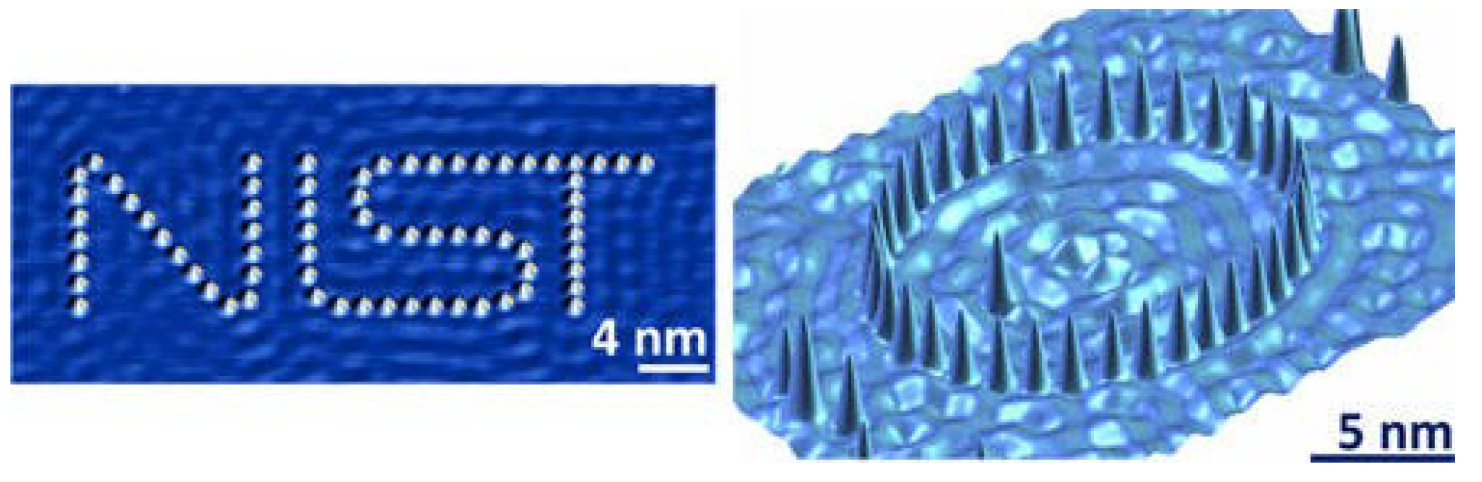
Any doping scheme should follow a repeated pattern to facilitate fabrication. The autonomous construction of the NIST trademark nanostructure is depicted on the left of Figure 2. Fluid electron “waves” on the copper material are produced by fluctuations on the Cu surface, which reflect the Co atoms. The reflected waves can provide patterns when the adatoms create the desired pattern, as seen by the elliptic border on the right side of the Figure 2.
The equation that defines the number of i repetitions of normal and inserted atoms the surface is:
In this type of model, there are several atoms on the moving surface, N, which coincides with several atoms on the fixed surface, M. Therefore, is equal to , where l is the atom–atom distance on the upper surface and is the distance between atoms on the fixed surface. For simplicity, is considered in this work to be equal to unity. We also consider the quotient, , to be an approximation of the golden number, , the incommensurable case. This number is approximated by a term of the Fibonacci series, namely 144/233. Thus, the mobile surface, N, is 233. The incommensurable case ensures that the critical rigidity is referred to as the Aubry transition [32]. When the stiffness exceeds the critical value, the atoms in the network make fast transitions.
With , Equation (4) can be written as:
One way to solve the equation is to consider the known variable . In the following, the equation will be solved for values of between 1 and 5. Thus, for , the result is:
Depending of N a fixing we can choose integer solutions of Equation (6). Since , . This means that and for each value of a value of i. An example of the election of the parameter is shown in Table 1.
If we opt for the solution and , we obtain the contamination pattern shown in Figure 1.
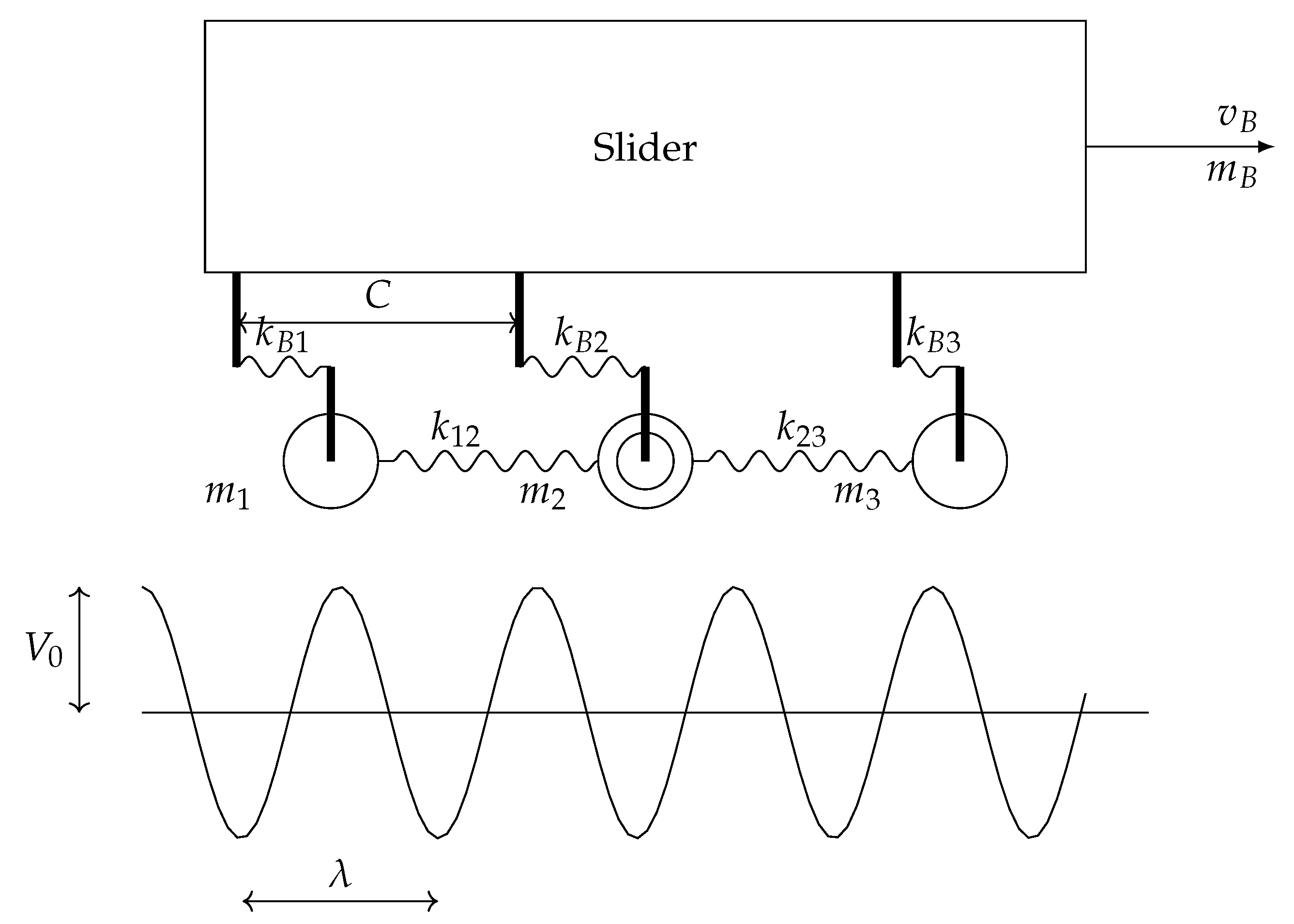
The problem to be solved on doped surfaces is made using the FKT approach. Figure 3 shows a scheme of this model. Springs reflect the atom–atom interaction in the top sliding body’s surface layer and their atom–atom relationship with the bulk. The interaction potential between these atoms and the reference surface of the relative motion is made by a trigonometric function.
Regarding a sliding surface atom noted with j and the relative displacement of the atom of mass m by , the inertial force is represented by . The viscous damping force associated with the absolute motion of the atom is represented by the terms and , and the elastic forces by and .
The force chosen to represent the interaction between atom j and the fixed surface is:
with j from 1 to N, we can set up an equation for each of the atoms as follows:
Or more generally, the balancing equation is:
From the ratio between the number of atoms of both surfaces, a boundary condition is established for the variation of the position of the first and last atom of this section. Thus, atom 1 and of the mobile surface must have equal relative variation with respect to their equilibrium positions:
This condition allows the model to be reduced to a system with N atoms.
From the above, the non-linear, one-dimensional model consists of a system of differential equations each associated with the atom j plus boundary conditions. All variables and all parameters are dimensionless; the stiffness/mass ratio unit is and the length unit is . The remaining units are referred to in terms of these fundamental units. The relative displacement of each of the N atoms results, the total non-stationary friction force for a constant moving surface velocity, , is defined by:
3. Network Simulation Method
The Network Simulation Method (NSM) [50,51,52] entails breaking down the investigated system into electrical circuits with identical governing equations. Electrical variables correspond to physical variables in the original system.
The physical problem will be addressed after the equations of the circuits are solved using classic numerical integration. As a result, NGSpice enables us to simulate electric circuits and analyse their responses.
Solano et al. [53,54] include a more extensive discussion of the precision of the NSM in some circumstances when convergence is difficult to obtain. Kirchoff’s rules and a suitable time step are used to solve the analogous electrical network for this approach, which assumes a steady convergence [55,56,57,58]. Several efforts have been dedicated to truncation error employing PSpice, which is where NGSpice acquires its name [59,60,61].
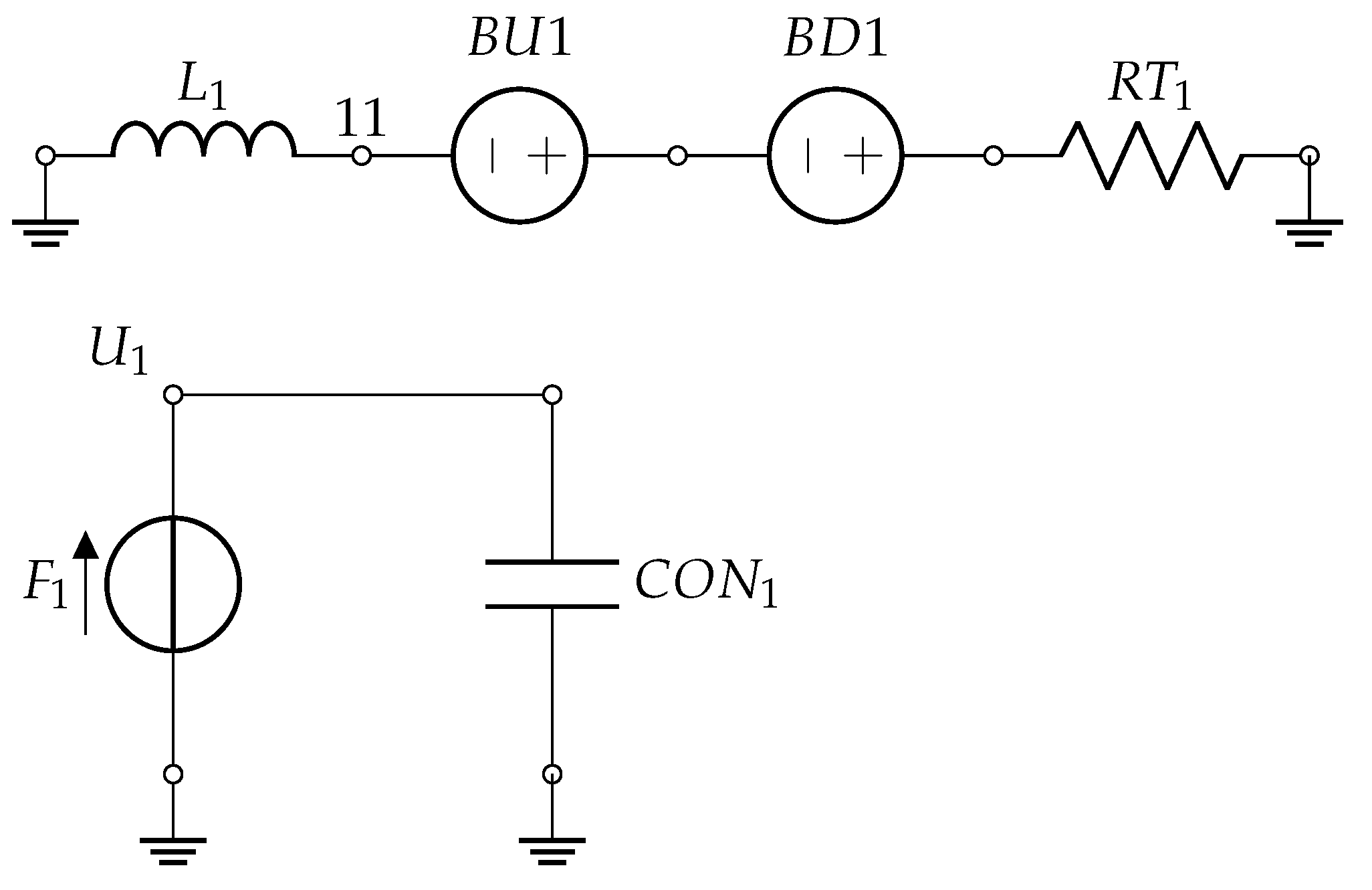
Figure 4 shows the circuits associated with the balance equation. In the left-hand circuit, the coil represents the inertial term, or first summand of Equation (9). The first voltage source represents the stiffness terms, the second voltage source represents the force associated with the interaction potential with the fixed surface, and the resistor represents the damping term. The bottom circuit performs the integration of the current by the top circuit, and the relative velocity of each atom, since the displacement value must be used in the first voltage source of the left-hand circuit.
4. Simulations and Results
The values of the parameters used in this paper follow the works of Weiss and Elmer [21,22]. Table 2 shows the design of experiments with four doping patterns and three values of as variables.
In a non-doped surface, the elastic force between the atoms is defined by the stiffness, , whose value has been chosen as 1.4, the same value used in a published article [54]. When we have a doped surface, the elastic force between the original atoms and the new one must be different, which is why we have chosen different stiffness values.
The values selected for the variable are typical of undoped surfaces showing the transition between chaotic and periodic behaviour.
The remaining parameters are , equal to 0.5, M/N, equal to 144/233, b/m, equal to 0.1, , equal to 1, , equal to zero and , equal to 0.1.
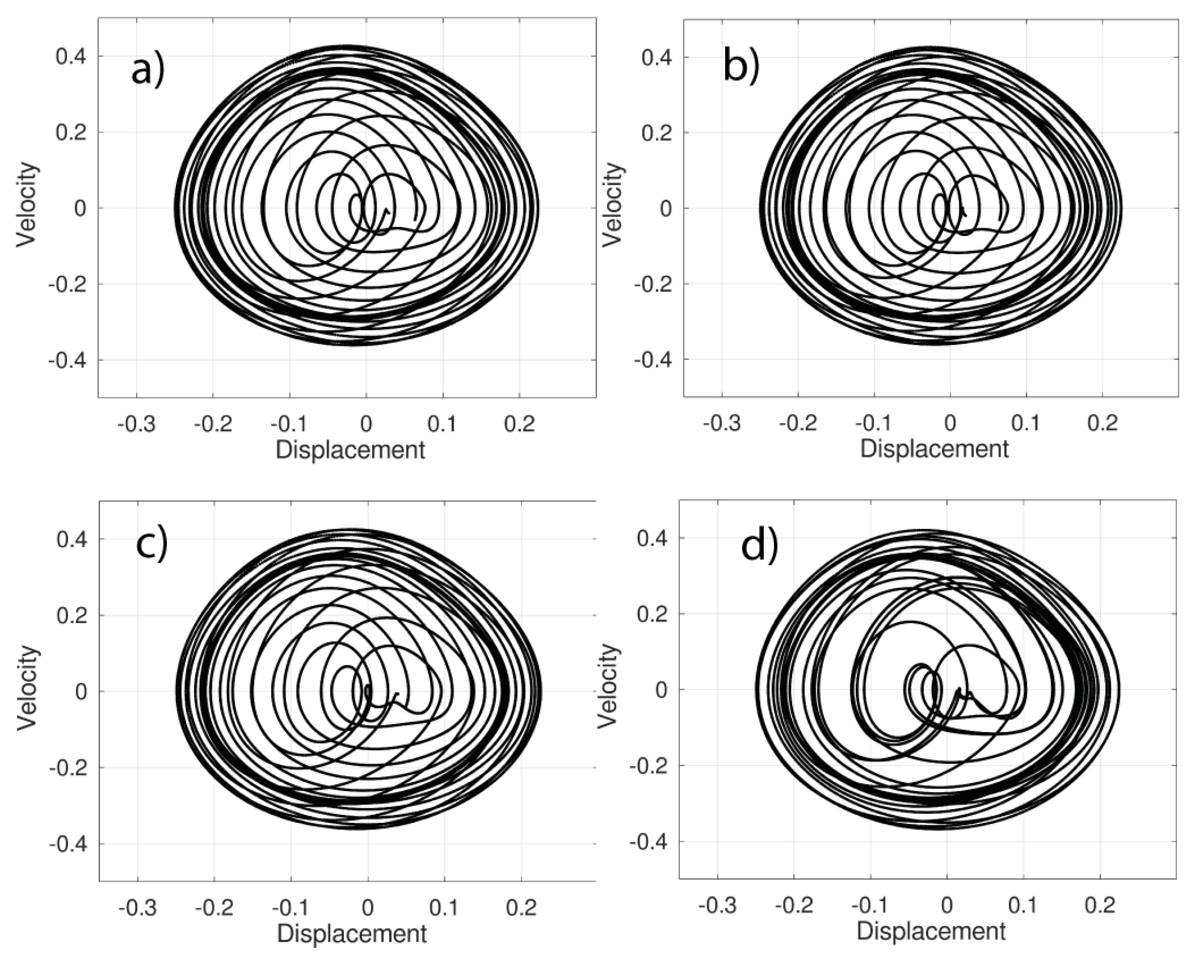
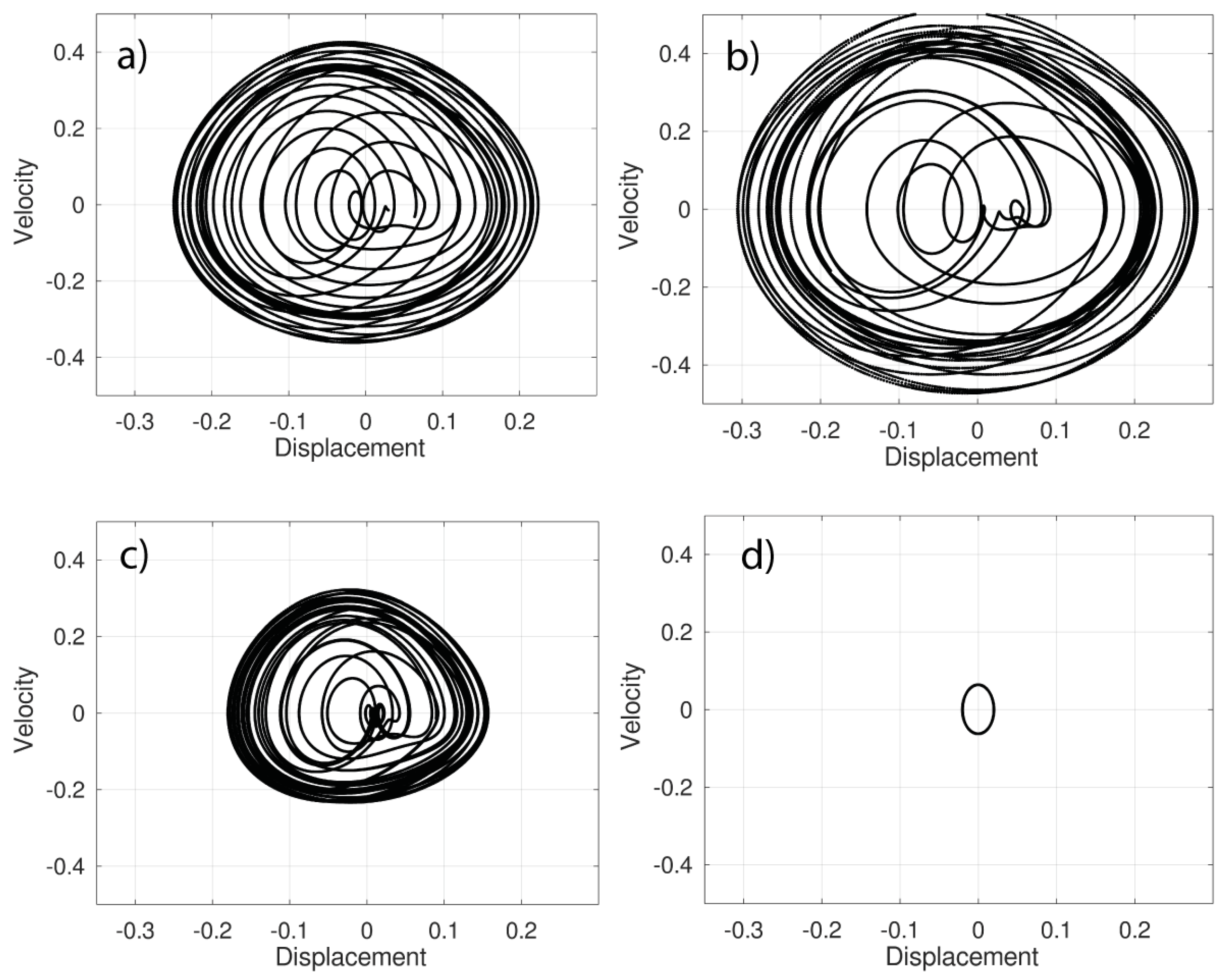
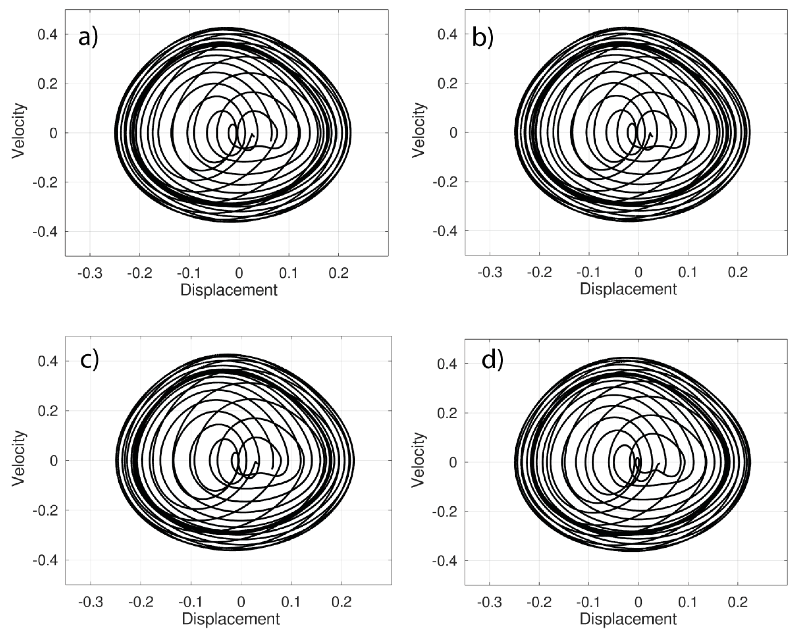
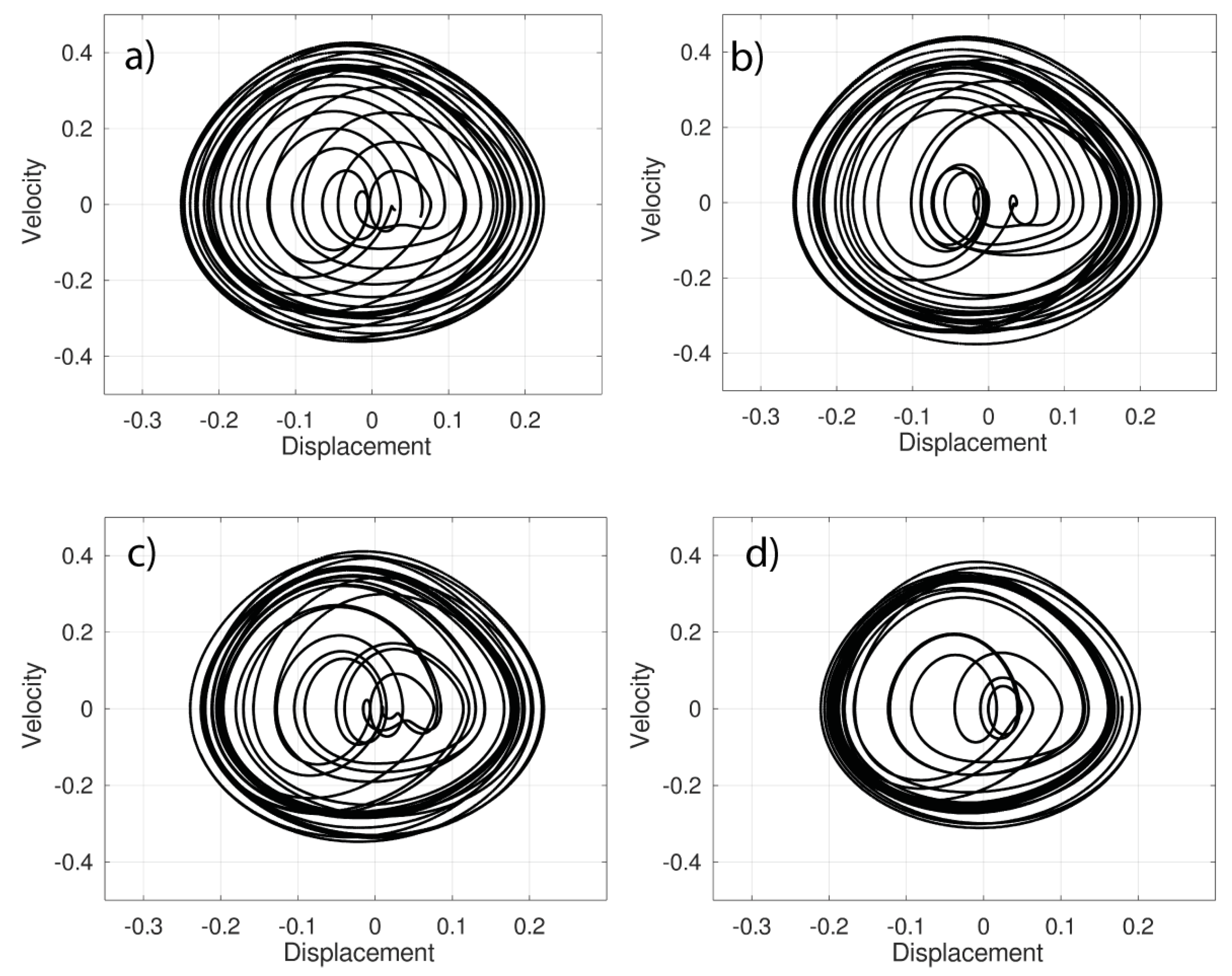
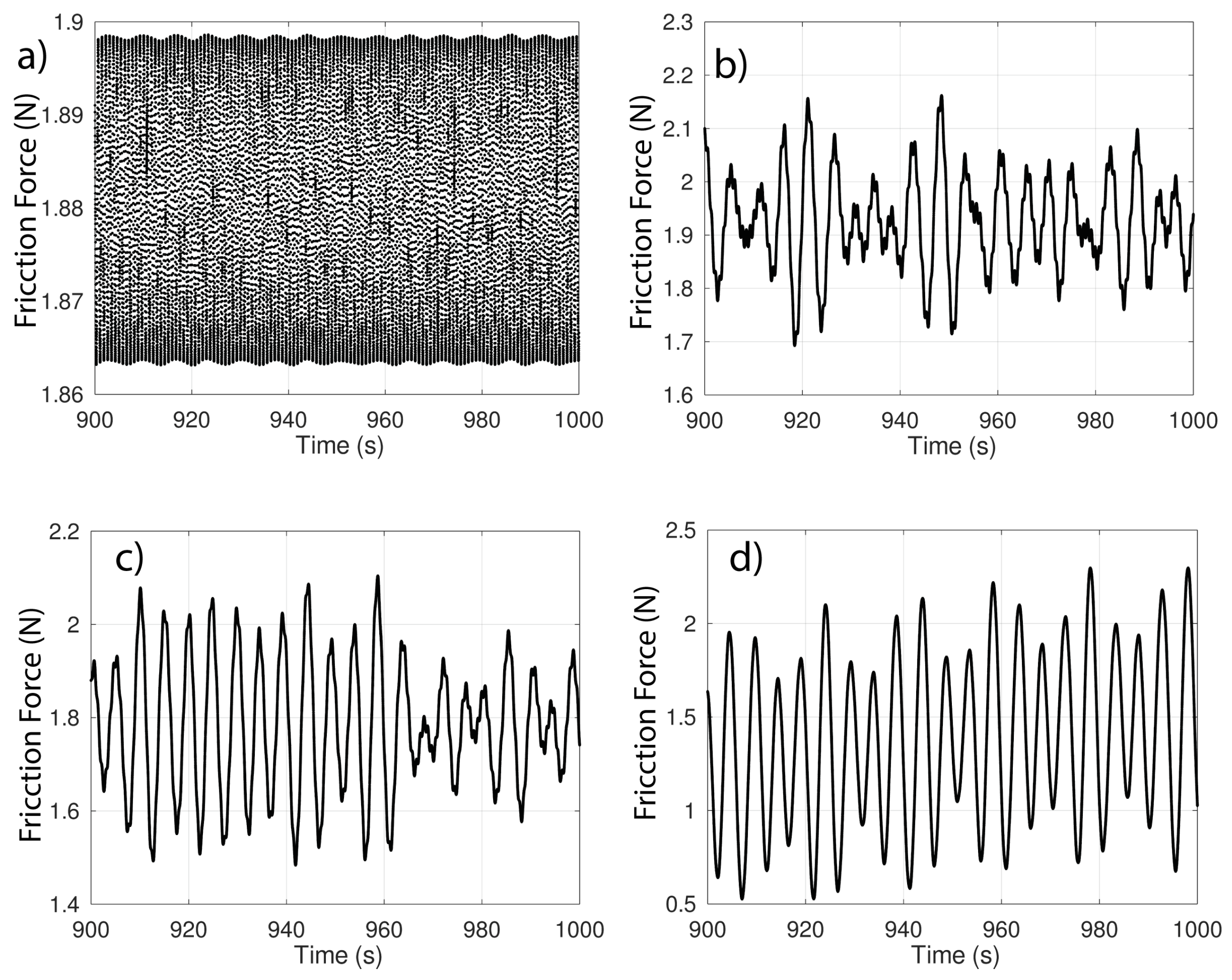
Figure 5, Figure 6, Figure 7 and Figure 8 show the phase diagrams for atom 55 without doping and with each of the doping types proposed in Table 2. Figure 9, Figure 10, Figure 11 and Figure 12 show the friction force without doping and with each of the doping types proposed in Table 3.
Table 3 shows the friction forces for undoped surfaces and for different doping patterns. The table shows that for the second doping pattern and , the highest friction force is achieved. However, with the same doping pattern and , the lowest friction force value is reached. In this case, the phase diagram indicates a behaviour.
In Figure 5, we can observe the transition between the value corresponding to 1.5, Figure 5c, and the value 1.7, Figure 5d. In Figure 5b,c we can see that the orbits are distributed in two clearly differentiated zones, the periphery and the interior, while in Figure 5d the orbits tend to overlap.
In Figure 6, the differences observed in Figure 5 are more evident. In addition, a change in size is evident, which is more abrupt in the transition between Figure 6c,d.
Figure 7 shows the two zones indicated in the comment to Figure 5: periphery and interior. This doping is not very sensitive to the variation of the parameter.
Figure 8 shows a similar behaviour to that of the system in Figure 5. However, the doping schemes corresponding to these figures, types 1 and 4, Table 2, are very different. In contrast, the doped types 1 and 3, which are very similar, show different behaviours.
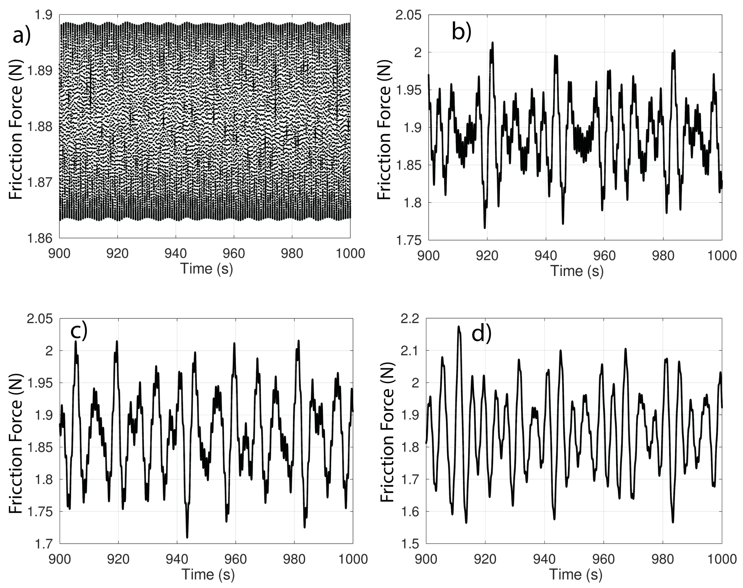
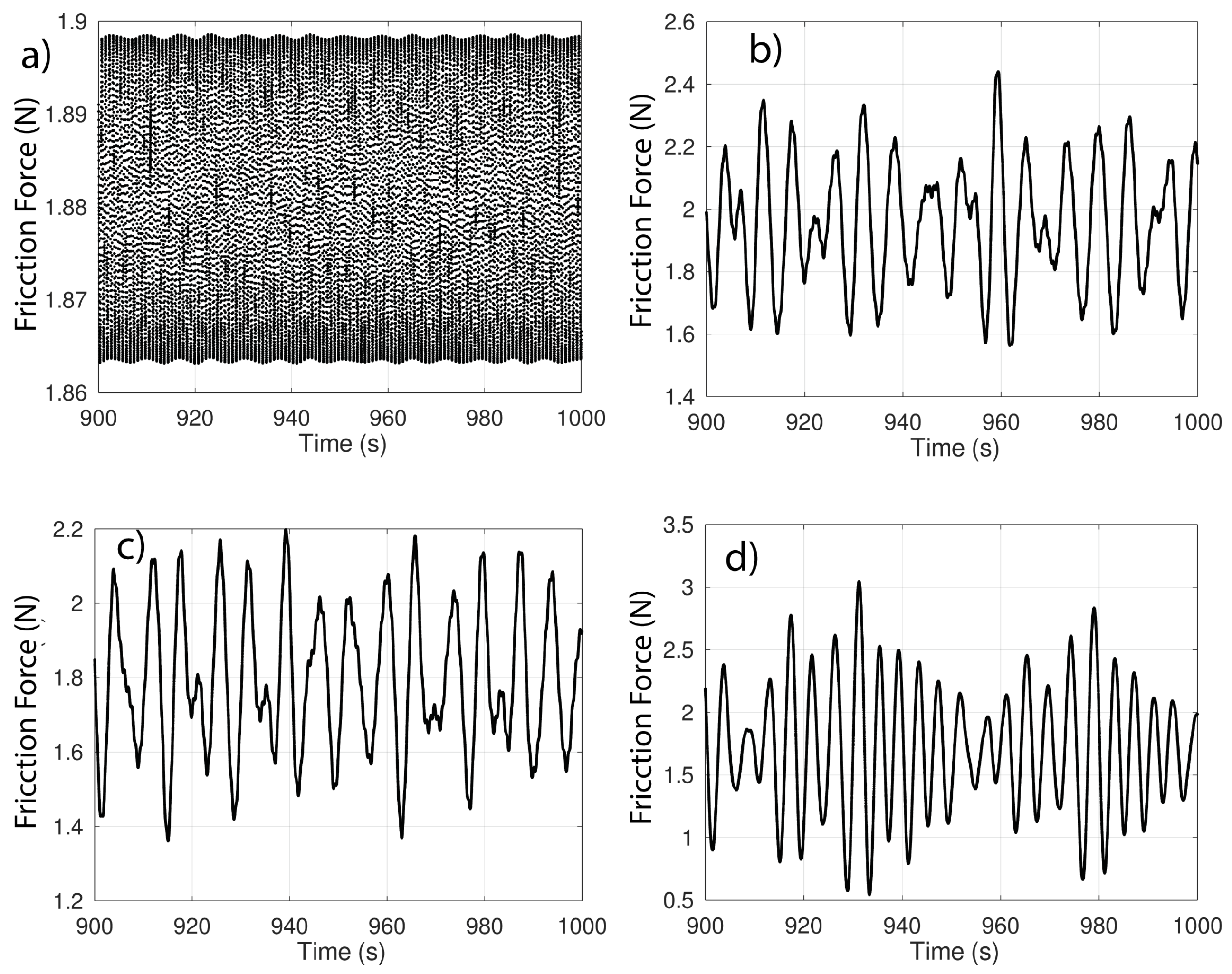
Figure 9, Figure 10, Figure 11 and Figure 12 show different values of the average friction force with varying amplitudes around this average value.
Figure 9 shows how the friction force decreases as the stiffness increases, but the amplitude of the oscillation increases. The increase in stiffness should result in an increase in friction force, but also a decrease in deflection, which in turn decreases the friction force. Therefore, the effect of the decrease in deformation outweighs the effect of the increase in stiffness.
In Figure 10, which corresponds to doping 2, the drop in friction force is more pronounced than for Figure 9, corresponding to doping 1.
Figure 11 shows almost no change in the friction force, with the oscillation amplitudes remaining practically in the same range for the different values of .
Figure 12 shows a decrease in friction force with stiffness, although the amplitudes of the oscillations increase.
The phase diagrams, Figure 5, Figure 6, Figure 7 and Figure 8, show two distinct zones for all stiffness values except for the second type of doping and the highest stiffness considered. Referring to Figure 9, Figure 10, Figure 11 and Figure 12, the increase in stiffness implies a decrease in friction force except for the third type of doping, where the decrease is negligible.
Table 3 shows the friction forces for surfaces without doping and for different doping patterns.
5. Conclusions
Understanding friction at the atomic scale is a helpful means for the improvement of mechanisms operating at these scales. In turn, it can serve as a reference for understanding the changes that occur when moving from the microscopic to the macroscopic scale.
In this study, surfaces with different doping patterns have been analysed and significant changes in frictional behaviour have been identified. This work shows the power of the models to minimize testing time under laboratory conditions. On the other hand, the ideal conditions used in these models can be used to identify doping pattern with low friction to be tested in laboratory conditions.
In terms of particular results, it is observed that an increase in the doping proportion, the second type of doping pattern proposed, can reduce the friction values as a function of the stiffness introduced.
It is evident that the doping pattern that uses more doping atoms provides the widest range of friction force values.
Author Contributions
J.S. Network simulation method, numerical simulation. F.B. Differential equations, dynamical system. J.A.M. Numerical simulation, network simulation method. F.M. Network simulation method, friction forces. All authors have read and agreed to the published version of the manuscript.
Funding
This research received no external funding.
Conflicts of Interest
The authors declare that they have no known competing financial interests or personal relationships that could have appeared to influence the work reported in this paper.
Abbreviations
The following abbreviations are used in this manuscript:
| FKT | Frenkel–Kontorova–Tomlinson model |
| PT | Prandtl–Tomlinson model |
| FK | Frenkel-Kontorova model |
| AFM | Atomic force microscope |
| SFM | Scanning force microscope |
| STM | Scanning tunneling microscope |
| PVD | Physical vapour deposition |
| VLSI | Very-large-scale integration |
| NSM | Network Simulation Method |
| FE | Forward-Euler |
| BE | Backward-Euler |
| LTE | Local truncation error |
| TR | Trapezoidal procedure |
References
- Jonsmann, J.; Sigmund, O.; Bouwstra, S. Compliant thermal microactuators. Sens. Actuators A Phys. 1999, 76, 463–469. [Google Scholar] [CrossRef]
- Mahalik, N.P. Micromanufacturing and Nanotechnology; Springer: Berlin/Heidelberg, Germany, 2006. [Google Scholar]
- Ouyang, X.; Tilley, D.; Keogh, P.; Yang, H.; Johnson, N.; Bowen, C.; Hopkins, P. Piezoelectric actuators for screw-in cartridge valves. In Proceedings of the 2008 IEEE/ASME International Conference on Advanced Intelligent Mechatronics, Xi’an, China, 2–5 July 2008; pp. 49–55. [Google Scholar]
- Engel, U.; Eckstein, R. Microforming—From basic research to its realization. J. Mater. Process. Technol. 2002, 125, 35–44. [Google Scholar] [CrossRef]
- Razali, A.R.; Qin, Y. A review on micro-manufacturing, micro-forming and their key issues. Procedia Eng. 2013, 53, 665–672. [Google Scholar] [CrossRef] [Green Version]
- Abtahi, M.; Vossoughi, G.; Meghdari, A. Dynamic Modeling of Scratch Drive Actuators. J. Microelectromech. Syst. 2015, 24, 1370–1383. [Google Scholar] [CrossRef]
- Fu, M.; Chan, W.L. A review on the state-of-the-art microforming technologies. Int. J. Adv. Manuf. Technol. 2013, 67, 2411–2437. [Google Scholar] [CrossRef]
- Singh, A.; Suh, K.Y. Biomimetic patterned surfaces for controllable friction in micro-and nanoscale devices. Micro Nano Syst. Lett. 2013, 1, 1–11. [Google Scholar] [CrossRef] [Green Version]
- Liu, Y.; Li, J.; Hu, X.; Zhang, Z.; Cheng, L.; Lin, Y.; Zhang, W. Modeling and control of piezoelectric inertia–friction actuators: Review and future research directions. Mech. Sci. 2015, 6, 95–107. [Google Scholar] [CrossRef] [Green Version]
- Schneider, J.; Djamiykov, V.; Greiner, C. Friction reduction through biologically inspired scale-like laser surface textures. Beilstein J. Nanotechnol. 2018, 9, 2561–2572. [Google Scholar] [CrossRef]
- Oscurato, S.L.; Salvatore, M.; Maddalena, P.; Ambrosio, A. From nanoscopic to macroscopic photo-driven motion in azobenzene-containing materials. Nanophotonics 2018, 7, 1387–1422. [Google Scholar] [CrossRef]
- Kumar, P.K.; Nithishkumar, D.; Gabriel, V.K.; Jerbin, J.; Joseph, J.J. Experimental study on frictional characteristics of alumina surface through biologically inspired catfish and shark fish scale like laser textures under dry and lubricating condition. In Proceedings of the AIP Conference Proceedings; AIP Publishing LLC: Melville, NY, USA, 2021; Volume 2417, p. 020006. [Google Scholar]
- Sharma, S.K.; Kodli, B.K.; Saxena, K.K. Micro forming and its applications: An overview. Key Eng. Mater. 2022, 924, 73–91. [Google Scholar] [CrossRef]
- Prandtl, L. Ein Gedankenmodell zur kinetischen Theorie der festen Körper. ZAMM-J. Appl. Math. Mech. Angew. Math. Und Mech. 1928, 8, 85–106. [Google Scholar] [CrossRef]
- Tomlinson, G. CVI. A molecular theory of friction. Lond. Edinburgh Dublin Philos. Mag. J. Sci. 1929, 7, 905–939. [Google Scholar] [CrossRef]
- Sánchez-Pérez, J.; Marín, F.; Morales, J.; Cánovas, M.; Alhama, F. Modeling and simulation of different and representative engineering problems using Network Simulation Method. PLoS ONE 2018, 13, e0193828. [Google Scholar] [CrossRef] [Green Version]
- Sircar, A.; Patra, P.K. A simple generalization of Prandtl–Tomlinson model to study nanoscale rolling friction. J. Appl. Phys. 2020, 127, 135102. [Google Scholar] [CrossRef] [Green Version]
- Kontorova, T.; Frenkel, J. On the theory of plastic deformation and twinning. II. Zh. Eksp. Teor. Fiz. 1938, 8, 1340–1348. [Google Scholar]
- Quapp, W.; Bofill, J.M. An Analysis of Some Properties and the Use of the Twist Map for the Finite Frenkel–Kontorova Model. Electronics 2022, 11, 3295. [Google Scholar] [CrossRef]
- Alhama, F.; Marín, F.; Moreno, J. An efficient and reliable model to simulate microscopic mechanical friction in the Frenkel–Kontorova–Tomlinson model. Comput. Phys. Commun. 2011, 182, 2314–2325. [Google Scholar] [CrossRef]
- Weiss, M.; Elmer, F.J. Dry friction in the Frenkel-Kontorova-Tomlinson model: Static properties. Phys. Rev. B 1996, 53, 7539. [Google Scholar] [CrossRef] [PubMed]
- Weiss, M.; Elmer, F.J. Dry friction in the Frenkel-Kontorova-Tomlinson model: Dynamical properties. Z. Phys. B Condens. Matter 1997, 104, 55–69. [Google Scholar] [CrossRef] [Green Version]
- Burridge, R.; Knopoff, L. Model and theoretical seismicity. Bull. Seismol. Soc. Am. 1967, 57, 341–371. [Google Scholar] [CrossRef]
- Carlson, J.M.; Langer, J. Properties of earthquakes generated by fault dynamics. Phys. Rev. Lett. 1989, 62, 2632. [Google Scholar] [CrossRef] [PubMed]
- Erickson, B.A.; Birnir, B.; Lavallée, D. Periodicity, chaos and localization in a Burridge–Knopoff model of an earthquake with rate-and-state friction. Geophys. J. Int. 2011, 187, 178–198. [Google Scholar] [CrossRef] [Green Version]
- Barbot, S. Slow-slip, slow earthquakes, period-two cycles, full and partial ruptures, and deterministic chaos in a single asperity fault. Tectonophysics 2019, 768, 228171. [Google Scholar] [CrossRef]
- Stefanou, I. Control instabilities and incite slow-slip in generalized Burridge-Knopoff models. arXiv 2020, arXiv:2008.03755. [Google Scholar]
- Awrejcewicz, J.; Olejnik, P. Stick-slip dynamics of a two-degree-of-freedom system. Int. J. Bifurc. Chaos 2003, 13, 843–861. [Google Scholar] [CrossRef]
- Galvanetto, U. Some discontinuous bifurcations in a two-block stick–slip system. J. Sound Vib. 2001, 248, 653–669. [Google Scholar] [CrossRef] [Green Version]
- Galvanetto, U.; Bishop, S. Characterisation of the dynamics of a four-dimensional stick-slip system by a scalar variable. Chaos Solitons Fractals 1995, 5, 2171–2179. [Google Scholar] [CrossRef]
- Van de Vrande, B.; Van Campen, D.; De Kraker, A. An approximate analysis of dry-friction-induced stick-slip vibrations by a smoothing procedure. Nonlinear Dyn. 1999, 19, 159–171. [Google Scholar] [CrossRef]
- Bishop, A. Solitons in condensed matter physics. Phys. Scr. 1979, 20, 409. [Google Scholar] [CrossRef]
- Schwarz, U.D.; Hölscher, H. Atomic-Scale Friction Studies Using Scanning Force Microscopy. In Modern Tribology Handbook, Two Volume Set; CRC Press: Boca Raton, FL, USA, 2000; pp. 671–696. [Google Scholar]
- Fan, P.; Goel, S.; Luo, X.; Upadhyaya, H.M. Atomic-scale friction studies on single-crystal gallium arsenide using atomic force microscope and molecular dynamics simulation. Nanomanuf. Metrol. 2021, 5, 39–49. [Google Scholar] [CrossRef]
- Hälg, D.; Gisler, T.; Tsaturyan, Y.; Catalini, L.; Grob, U.; Krass, M.D.; Héritier, M.; Mattiat, H.; Thamm, A.K.; Schirhagl, R.; et al. Membrane-based scanning force microscopy. Phys. Rev. Appl. 2021, 15, L021001. [Google Scholar] [CrossRef]
- Meyer, E.; Heinzelmann, H. Scanning force microscopy (SFM). In Scanning Tunneling Microscopy II; Springer: Berlin/Heidelberg, Germany, 1995; pp. 99–149. [Google Scholar]
- Ducourtieux, S.; Poyet, B. Development of a metrological atomic force microscope with minimized Abbe error and differential interferometer-based real-time position control. Meas. Sci. Technol. 2011, 22, 094010. [Google Scholar] [CrossRef]
- Greenwood, J. Fundamentals of friction. In Macroscopic and Microscopic Processes; Springer Science and Business Media, B.V.: Berlin/Heidelberg, Germany, 1992. [Google Scholar]
- Greenwood, J.A.; Williamson, J.P. Contact of nominally flat surfaces. Proc. R. Soc. Lond. Ser. A Math. Phys. Sci. 1966, 295, 300–319. [Google Scholar]
- Myshkin, N.; Grigoriev, A.Y.; Chizhik, S.; Choi, K.; Petrokovets, M. Surface roughness and texture analysis in microscale. Wear 2003, 254, 1001–1009. [Google Scholar] [CrossRef]
- Manabe, K.-i. Metal Micro-Forming. Metals 2020, 10, 813. [Google Scholar] [CrossRef]
- Bučinskas, V.; Subačiūtė-Žemaitienė, J.; Dzedzickis, A.; Morkvėnaitė-Vilkončienė, I. Robotic micromanipulation: A) actuators and their application. Robot. Syst. Appl. 2021, 1, 2–23. [Google Scholar] [CrossRef]
- Gibbons, J.F. Ion implantation in semiconductors—Part I: Range distribution theory and experiments. Proc. IEEE 1968, 56, 295–319. [Google Scholar] [CrossRef]
- Stroscio, J.A.; Celotta, R.J. Controlling the dynamics of a single atom in lateral atom manipulation. Science 2004, 306, 242–247. [Google Scholar] [CrossRef] [PubMed] [Green Version]
- Manova, D.; Gerlach, J.W.; Mändl, S. Thin film deposition using energetic ions. Materials 2010, 3, 4109–4141. [Google Scholar] [CrossRef] [PubMed] [Green Version]
- Mundra, S.; Pardeshi, S.; Bhavikatti, S.; Nagras, A. Development of an integrated physical vapour deposition and chemical vapour deposition system. Mater. Today Proc. 2021, 46, 1229–1234. [Google Scholar] [CrossRef]
- Kizu, R.; Misumi, I.; Hirai, A.; Kinoshita, K.; Gonda, S. Development of a metrological atomic force microscope with a tip-tilting mechanism for 3D nanometrology. Meas. Sci. Technol. 2018, 29, 075005. [Google Scholar] [CrossRef]
- Misumi, I.; Sugawara, K.; Kizu, R.; Hirai, A.; Gonda, S. Extension of the range of profile surface roughness measurements using metrological atomic force microscope. Precis. Eng. 2019, 56, 321–329. [Google Scholar] [CrossRef]
- Sun, L.; Wang, Q.J.; Zhao, N.; Zhang, M. Discrete convolution and FFT modified with double influence-coefficient superpositions (DCSS–FFT) for contact of nominally flat heterogeneous materials involving elastoplasticity. Comput. Mech. 2021, 67, 989–1007. [Google Scholar] [CrossRef]
- Peusner, L. The Principles of Network Thermodynamics: Theory and Biophysical Applications. Ph.D. Thesis, Harvard University, Cambridge, MA, USA, 1970. reprinted by Entropy, Lincoln, MA, USA, 1987. [Google Scholar]
- Nagel, L.W. SPICE2: A Computer Program to Simulate Semiconductor Circuits. Ph.D. Thesis, University of California, Berkeley, CA, USA, 1975. [Google Scholar]
- Nagel, L.; Pederson, D. Simulation program with integrated circuit emphasis. In Proceedings of the Midwest Symposium on Circuit Theory, Waterloo, ON, Canada, 12 April 1973. [Google Scholar]
- Solano, J.; Balibrea, F.; Moreno, J.A. Applications of the Network Simulation Method to Differential Equations with Singularities and Chaotic Behaviour. Mathematics 2021, 9, 1442. [Google Scholar] [CrossRef]
- Solano, J.; Balibrea, F.; Moreno, J.A.; Marín, F. Analysis of Chaotic Response of Frenkel-Kontorova-Tomlinson Model. Symmetry 2020, 12, 1413. [Google Scholar]
- Andreev, V.; Ostrovskii, V.; Karimov, T.; Tutueva, A.; Doynikova, E.; Butusov, D. Synthesis and Analysis of the Fixed-Point Hodgkin–Huxley Neuron Model. Electronics 2020, 9, 434. [Google Scholar] [CrossRef] [Green Version]
- Kaplun, D.I.; Tutueva, A.V.; Butusov, D.N.; Karimov, A.I.; Toming, J. Memristive Circuit Simulation Using the Semi-Implicit Multistep Method. In Proceedings of the 2019 42nd International Conference on Telecommunications and Signal Processing (TSP), Budapest, Hungary, 1–3 July 2019; pp. 98–101. [Google Scholar]
- Leonov, G.A.; Kuznetsov, N.V. Time-varying linearization and the Perron effects. Int. J. Bifurc. Chaos 2007, 17, 1079–1107. [Google Scholar] [CrossRef] [Green Version]
- Tutueva, A.; Butusov, D.; Okhota, A.; Pesterev, D.; Rodionova, E. The dynamical analysis of the modified rossler system. In Proceedings of the IOP Conference Series: Materials Science and Engineering; IOP Publishing: Bristol, UK, 2019; Volume 630, p. 012006. [Google Scholar]
- Vladimirescu, A. The SPICE Book; Wiley: Hoboken, NJ, USA, 1994. [Google Scholar]
- Skowronn, D.; Li, D.; Tymerski, R. Simulation of networks with ideal switches. Int. J. Electron. 1994, 77, 715–730. [Google Scholar] [CrossRef]
- Constantinescu, F.; Gheorghe, A.G.; Nițescu, M. The energy balance error for circuit transient analysis. Rev. Roum. Sci. Techn.–Électrotechn. Énerg. 2010, 55, 243–250. [Google Scholar]
Figure 1.
Doping pattern corresponding to (empty circles) and (circles with an inner circle).

Figure 2.
Nanostructure with the NIST logo made of Co atoms on a copper surface (left). Elliptic quantum fence manufactured with Co atoms on the Cu (111) layer (right). Source: NIST.
Figure 2.
Nanostructure with the NIST logo made of Co atoms on a copper surface (left). Elliptic quantum fence manufactured with Co atoms on the Cu (111) layer (right). Source: NIST.

Figure 3.
Schematic diagram of the FKT model.

Figure 4.
Balancing equation circuits (top) and integrator (bottom).

Figure 5.
Phase diagram: no doping with (a), and first type of doping with (b), (c) and (d).

Figure 6.
Phase diagram: no doping with (a), and second type of doping with (b), (c) and (d).

Figure 7.
Phase diagram: no doping with (a), and third type of doping with (b), (c) and (d).

Figure 8.
Phase diagram: no doping with (a), and fourth type of doping with (b), (c) and (d).

Figure 9.
Friction force: no doping with (a), and first type of doping with (b), (c) and (d).

Figure 10.
Friction force: no doping with (a), and second type of doping with (b), (c) and (d).

Figure 11.
Friction force: no doping with (a), and third type of doping with (b), (c) and (d).

Figure 12.
Friction force: no doping with (a), and fourth type of doping with (b), (c) and (d).


Table 1.
Values of i and for .
| i | |
|---|---|
| 1 | 116 |
| 3 | 58 |
| 7 | 29 |
| 28 | 8 |
| 57 | 4 |
| 115 | 2 |
| 231 | 1 |
Table 2.
Doping patterns in the FKT model and values of .
| Type of Doping | a | b | j | |
|---|---|---|---|---|
| 1 | 114 | 5 | 1 | 1.3 |
| 114 | 5 | 1 | 1.5 | |
| 114 | 5 | 1 | 1.7 | |
| 2 | 1 | 1 | 116 | 1.3 |
| 1 | 1 | 116 | 1.5 | |
| 1 | 1 | 116 | 1.7 | |
| 3 | 116 | 1 | 1 | 1.3 |
| 116 | 1 | 1 | 1.5 | |
| 116 | 1 | 1 | 1.7 | |
| 4 | 25 | 1 | 8 | 1.3 |
| 25 | 1 | 8 | 1.5 | |
| 25 | 1 | 8 | 1.7 |
Table 3.
Average friction force without and with four types of doping.
| Average Friction Force | ||
|---|---|---|
| Type of Doping | Friction Force | |
| Without doping | - | 1.880 |
| 1 | 1.3 | 1.880 |
| 1.5 | 1.880 | |
| 1.7 | 1.880 | |
| 2 | 1.3 | 3.1295 |
| 1.5 | 0.8913 | |
| 1.7 | ||
| 3 | 1.3 | 1.8885 |
| 1.5 | 1.8696 | |
| 1.7 | 1.8475 | |
| 4 | 1.3 | 1.9542 |
| 1.5 | 1.7933 | |
| 1.7 | 1.7709 | |
Disclaimer/Publisher’s Note: The statements, opinions and data contained in all publications are solely those of the individual author(s) and contributor(s) and not of MDPI and/or the editor(s). MDPI and/or the editor(s) disclaim responsibility for any injury to people or property resulting from any ideas, methods, instructions or products referred to in the content. |
© 2023 by the authors. Licensee MDPI, Basel, Switzerland. This article is an open access article distributed under the terms and conditions of the Creative Commons Attribution (CC BY) license (https://creativecommons.org/licenses/by/4.0/).
Share and Cite
MDPI and ACS Style
Solano, J.; Balibrea, F.; Moreno, J.A.; Marín, F. Dry Friction Analysis in Doped Surface by Network Simulation Method. Mathematics 2023, 11, 1341. https://doi.org/10.3390/math11061341
AMA Style
Solano J, Balibrea F, Moreno JA, Marín F. Dry Friction Analysis in Doped Surface by Network Simulation Method. Mathematics. 2023; 11(6):1341. https://doi.org/10.3390/math11061341
Chicago/Turabian StyleSolano, Joaquín, Francisco Balibrea, José Andrés Moreno, and Fulgencio Marín. 2023. "Dry Friction Analysis in Doped Surface by Network Simulation Method" Mathematics 11, no. 6: 1341. https://doi.org/10.3390/math11061341
Note that from the first issue of 2016, this journal uses article numbers instead of page numbers. See further details here.