
Numerical Study on the Orthogonality of the Fields Radiated by an Aperture
by
 , , , and
Lucas Polo-López
1,2,
Juan Córcoles
2,
Jorge A. Ruiz-Cruz
2,*,
José R. Montejo-Garai
3 and
Jesús M. Rebollar
3 1
Institut d’Electronique et des Technologies du numéRique (IETR), UMR CNRS 6164, INSA Rennes, 35700 Rennes, France
2
Group of RadioFrequency: Circuits and Systems (RFCAS), Escuela Politécnica Superior, Universidad Autónoma de Madrid, 28049 Madrid, Spain
3
Information Processing and Telecommunications Center, Universidad Politécnica de Madrid, 28040 Madrid, Spain
*
Author to whom correspondence should be addressed.
Mathematics 2023, 11(5), 1198; https://doi.org/10.3390/math11051198
Submission received: 3 January 2023
/
Revised: 21 February 2023
/
Accepted: 24 February 2023
/
Published: 28 February 2023
(This article belongs to the Special Issue Mathematical Modeling and Numerical Analysis for Applied Sciences)
Abstract
:This work studies the orthogonality of the fields radiated by the different modes of a radiating aperture. Waveguide modes exhibit an orthogonality property at the aperture cross-section that can be used to simplify calculations. However, it is unclear whether this property can be extended to the radiated fields produced by these same modes in apertures antennas, such as horns or open-ended waveguides. A numerical study has been carried out, analysing how the waveguide orthogonality extends to the radiated modal fields. It is observed that propagating modes and also modes that are well below cutoff follow this same behaviour. However, modes that are close to cutoff exhibit values in between those far from this transition region.
1. Introduction
Aperture antennas can take several forms, such as horns, reflectors, or slots, among others. Hence, thanks to this flexibility, they can be used in a wide range of different micro- and milli-metre-wave wireless systems [1,2]. The increasing demand in the performance for these kind of systems makes it necessary to develop efficient modelling strategies that allow us to create sophisticated designs, which obtain the best possible characteristics [3,4,5,6,7,8].
These efficient modelling techniques are based on having a deep understanding of the electromagnetic problem under study, with the objective of exploiting symmetries or orthogonality properties that may appear in order to reduce the computation times.
Several analysis and synthesis techniques [9,10,11,12,13,14] perform a modal expansion of the aperture field distribution in order to compute the total radiated field as the summation of the fields radiated by each modal field function weighted by their corresponding complex modal amplitudes. As is well known, these modal fields are orthogonal between them, since they constitute an orthogonal basis for the fields at the aperture [15]. Nevertheless, to the best of the author’s knowledge, it has not been addressed by the literature whether this orthogonality is also satisfied by their corresponding radiated fields.
In order to address this subject, the present work shows, first, the formulation to perform the modal expansion of the aperture radiated fields and then presents several numerical examples to assess the orthogonality of the radiated fields.
2. Modal Expansion of the Far-Field Produced by a Radiating Aperture
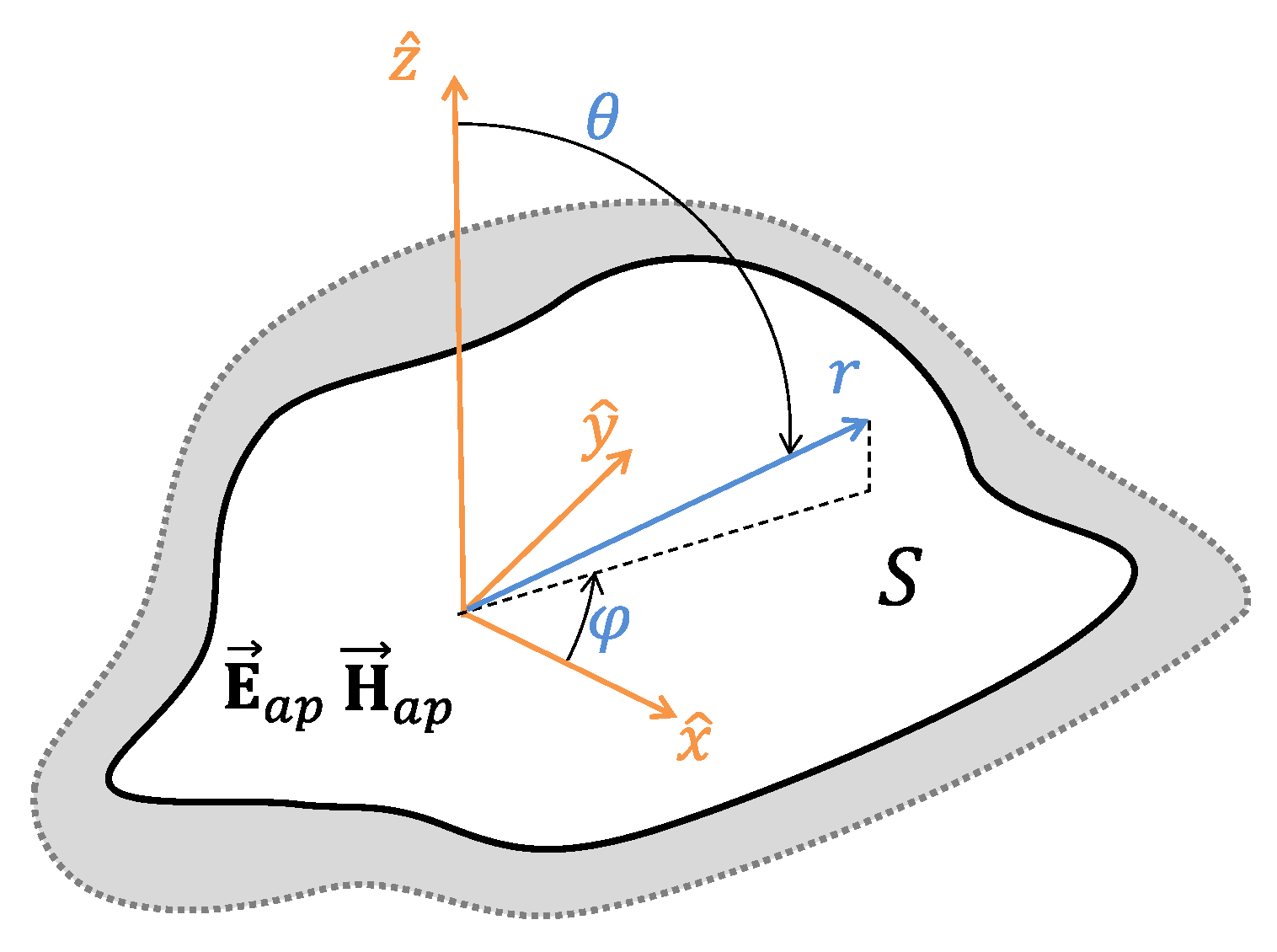
The field radiated by an aperture lying on the -plane, similar to the one depicted in Figure 1, can be computed from the transverse components of the electromagnetic field at the aperture using the well known equivalence principle [16] (Ch. 7) [17], denoted here by the linear integral operator, , as:
Please note that refer to a two-dimensional coordinate system used to calculate the transverse electromagnetic field at the aperture, while correspond to the tridimensional coordinate system used to express the radiated fields (as illustrated in Figure 1). Three different formulations of this equivalence principle () exist, depending on which type of currents are considered as a radiation source. As is well known, the accuracy of the equivalence principle is proportional to the aperture size ([16], Ch. 7 and [17]).
If both electric and magnetic currents are considered (alternative versions of these formulas can be obtained if only electric or only magnetic currents are considered as the radiation source), the equivalence principle in (1) takes the form:
where and represent the two-dimensional Fourier transform of the transversal electric and magnetic fields at the aperture S [16] (Ch. 7) (the x and y subscripts denote that the Fourier transform is computed for the x or y component of the field):
where is the free space wavenumber, is the free space magnetic permeability, is the free space electric permittivity, is the free space intrinsic impedance, S is the aperture surface in Figure 1, are the spherical coordinates with their standard definition, and , .
Nevertheless, instead of operating directly with the total fields at the aperture, it is more convenient to write them as the weighted sum of modal functions corresponding to a waveguide with a section S equal to the aperture geometry [15] (Ch. 3):
where represents the complex amplitudes of the electric () and magnetic () fields of the m-th mode, which can be computed as:
The term represents the mode impedance and is an arbitrary normalization constant. Additionally, the scalar function (which is real valued and frequency independent) is proportional to the longitudinal component of either the magnetic or electric field, depending on whether the m-th mode is transverse electric (TE) or transverse magnetic (TM). This function, which is assumed here to be normalized as , can be calculated by solving the Helmholtz equation with the adequate boundary conditions imposed by the aperture geometry [15]. For this work, they are considered known, calculated either analytically (as in the circular and squared cases) or numerically (represented, without loss of generality, by a polygonal case). The summation (4) is usually ordered by the cutoff frequency of the modes [15], and thus, each mode is identified by a single index m, its cutoff wavenumber is identified by , and its cutoff frequency by .
Certain waveguide geometries present analytical solutions for the modal fields. This is the case, for example, of circular and rectangular waveguides. The following expressions can be obtained to calculate the TE and TM modes of a circular waveguide of radius r:
with roots [18] (Ch. 9) and normalization constants:
for TE and TM modes, respectively. Please note that the formulas consider a standard polar coordinate system () whose origin is placed at the centre of the waveguide ().
Additionally, the following formulas can be derived for the TE and TM modes, respectively, of a rectangular waveguide in a system whose origin is at the centre of the rectangle:
with cut-off wavenumbers and normalization constants:
where a and b are, respectively, the width and height of the waveguide. It must be emphasized that the modal expansion can also be applied to waveguide geometries that do not present closed-form expressions for their modal field functions by calculating these modal fields numerically.
Therefore, thanks to this modal expansion and taking into consideration that the transformation denoted by is linear, (1) can be rewritten as:
where denotes the electric field radiated by the m-th mode:
Hence, the equivalence principle (2) can be applied to the electromagnetic field at the aperture on a modal basis; that is, the field radiated by each mode is computed independently, and then the total radiated field is obtained as the combination of the different , weighted by their corresponding modal amplitudes [12,13].
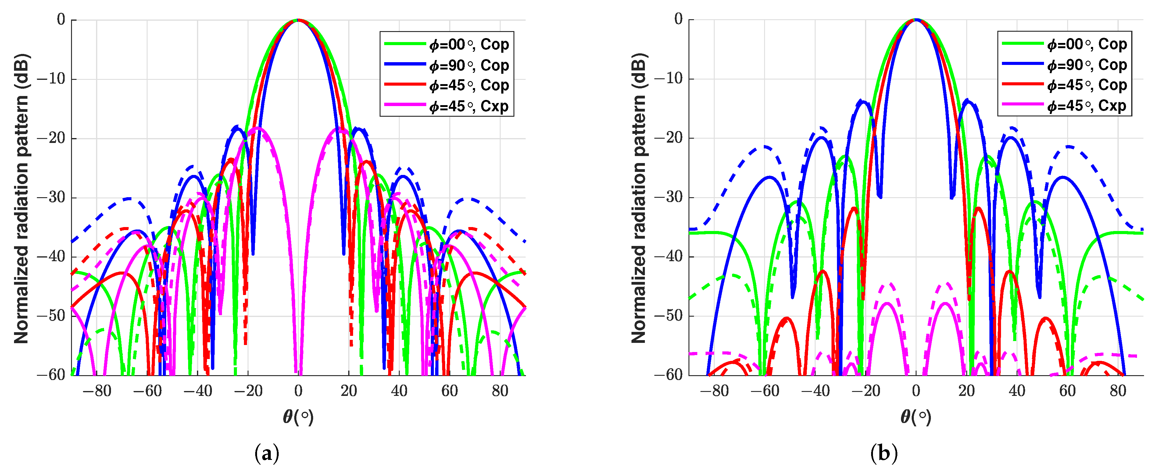
In order to verify this approach to calculate the radiated field produced by a modal field function, the obtained results have been compared with those provided by a third party commercial electromagnetic simulation software [19]. As an example, Figure 2 shows the radiation pattern corresponding to the fundamental mode of both a circular (radius ) an a squared aperture (side ). It can be observed that there is a good correspondence between both sets of results.
3. Radiated Field Cross-Products Matrix
The total power radiated by any antenna () can be computed from the integration of the radiated electric field [20] as:
It should be noted that the integration is calculated over an hemispheric surface, since the equivalence principle assumes that the aperture is placed on an infinite ground plane, and, therefore, it radiates only towards the free space region at one of the sides of such plane. Then, by applying (14), the former equation can be expressed using matrix notation:
where H denotes the Hermitian operator (transpose conjugate) and is the vector of complex modal amplitudes . Hence, knowing the matrix of the radiated field cross-products for a certain aperture geometry, it is possible to determine the power radiated by any field distribution at that aperture with the Hermitian quadratic form in (17).
4. Numerical Study of the Orthogonality for the Radiated Fields of Each Mode
The modal fields in (5) and (6) present the following orthogonality property [15] (Ch. 5) defined over the aperture surface S:
where is the Kronecker delta. Using (5) and (6), it can be easily shown that, for propagating modes (i.e., ), .
Moreover, when modes in (5) and (6) are written with (typical scenario that will be used later), is equal to 1 for propagating modes.
However, it is unclear if this same orthogonality is also exhibited by the fields (15) radiated by these modes, i.e., whether the following equation holds true:
The value of (18) for the fields radiated by an arbitrarily shaped aperture can be obtained with a good computational efficiency using a numerical approach based on the Lebedev-Laikov quadrature [21]. This technique approximates the value of a surface integral over a sphere as a weighted summation of different evaluations of the function to integrate over a grid of N points. Each evaluation of the function is weighted in the summation by a quadrature coefficient associated to the grid point , given by [21], where the function is evaluated, which are specified by the corresponding quadrature rule. Therefore, can be approximated as:
where and are defined as:
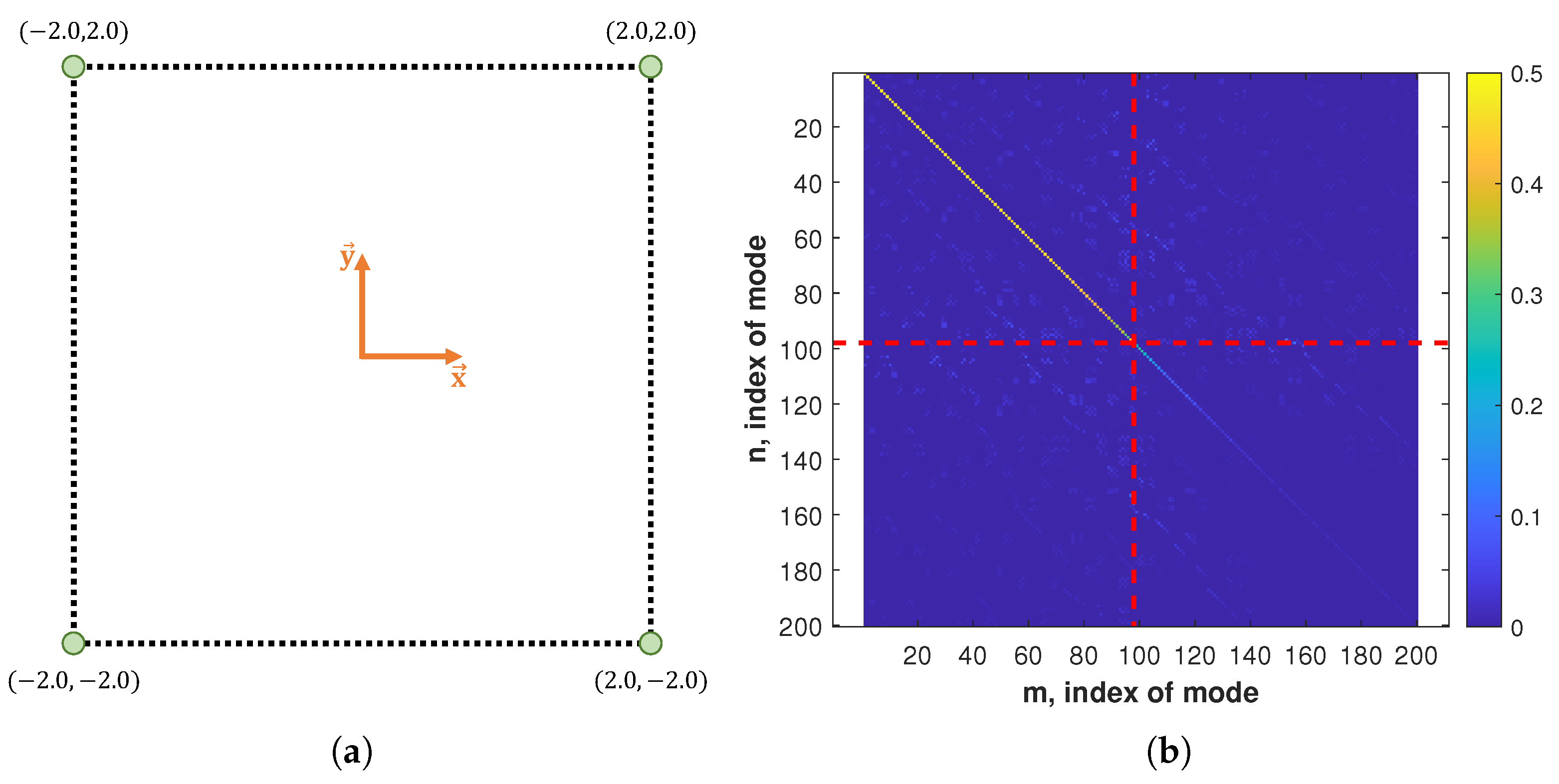
Then, it is possible to evaluate (21) for different aperture geometries. For example a typical circular aperture with a radius of , as illustrated in Figure 3a. For this geometry, Figure 3b displays a graphical representation of .
Two significant facts can be observed in these data. First of all, it can be seen that evanescent modes (mode number 78 and subsequent) present a decreasing contribution to the radiated power, which becomes smaller with the mode order. In addition, it can be observed that the submatrix corresponding to the propagating modes is almost a diagonal matrix, with the elements outside of the diagonal being almost zero. The average of the elements outside of the main diagonal is , while the average value for the elements in the main diagonal corresponding to the propagative modes is 0.49.
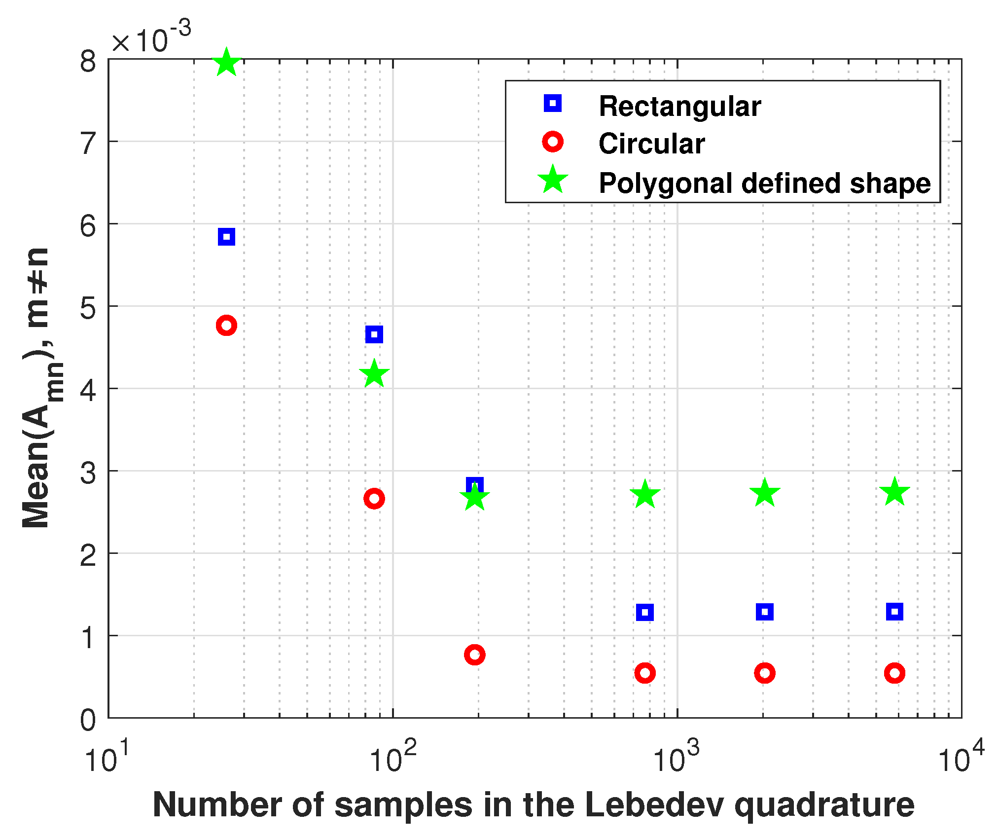
Indeed, the fact that the off-diagonal elements are not exactly zero can be explained by the convergence of the Lebedev-Laikov quadrature. The presented results have been obtained with a Lebedev-Laikov scheme of (which is the greatest possible number of points as defined in [21]). However, it has been checked that, when using grids with fewer points, these off-diagonal elements take higher values that progressively diminish when increasing the number of points at the grid, as shown in Figure 4.
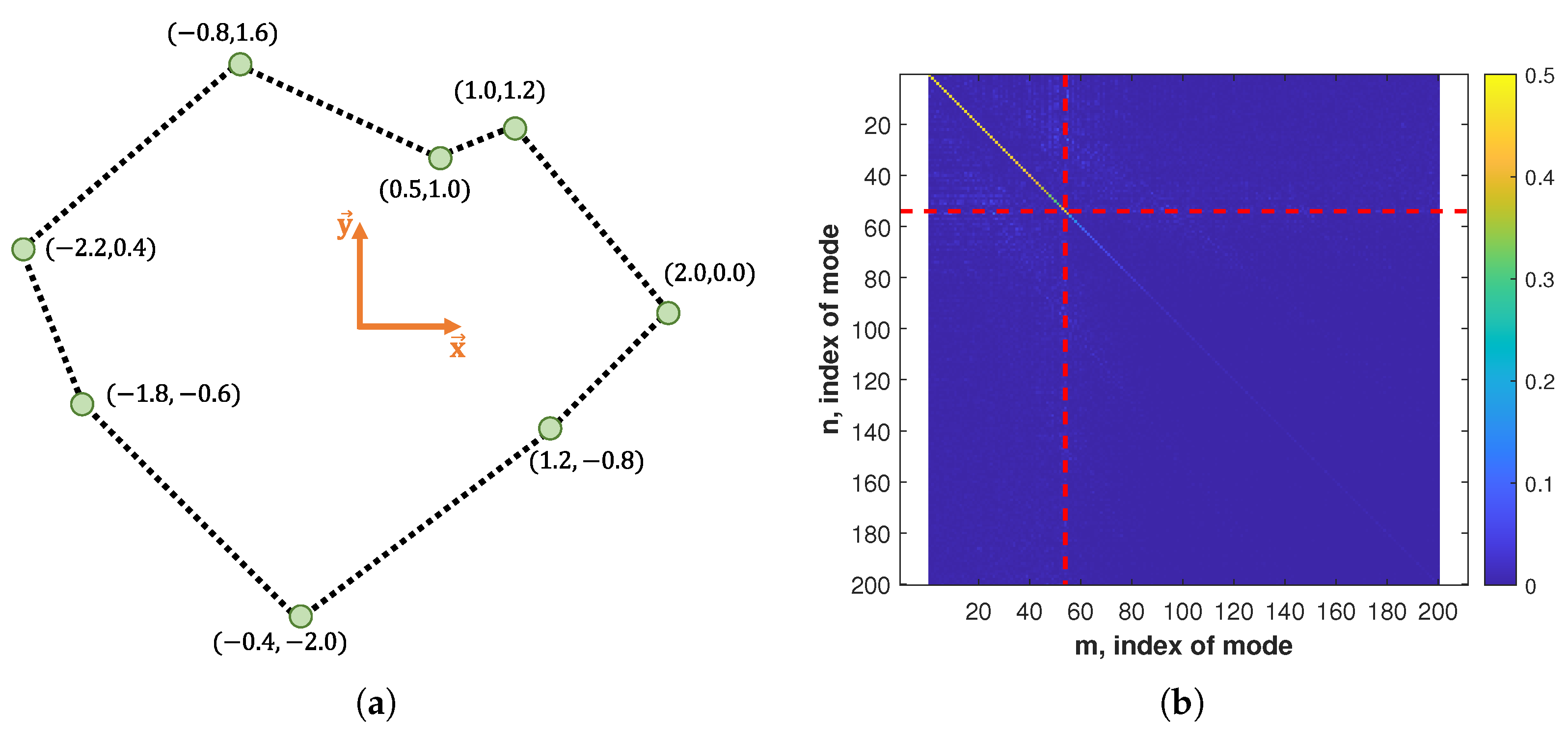
This matrix has also been computed for other aperture geometries. Figure 5b shows the results obtained for a squared aperture with a side , such as the one depicted in Figure 5a. As it can be appreciated, this aperture geometry exhibits a behaviour similar to the circular one, and the average of the off-diagonal elements is , while the average of the main diagonal elements is 0.49. In addition, in order to study the orthogonality in a geometry that does not present any symmetries, the aperture of Figure 6a [12] is analysed. The obtained matrix is represented in Figure 6b and, as it can be observed, it presents the same diagonal pattern as the circular and squared cases (average value of off-diagonal elements equal to and average value of diagonal elements equal to 0.45). The study of the convergence of the Lebedev-Laikov quadrature has also been carried out for these two geometries, and the results are also depicted in Figure 4. As it can be observed, for the squared and polygonal apertures, the average value of the off-diagonal elements also diminishes when the number of points in the quadrature is increased, as it happened for the circular aperture case.
Finally, Table 1 presents the numeric values of the main diagonal of for the three studied apertures. Since this matrix presents an elevated number of elements, three subsets of values are presented for each aperture: propagating modes, modes that are well below cutoff, and modes that are in the transition region between propagation and cutoff. As it can be observed, the elements in the main diagonal of do indeed follow (20) when the modes are either well above cutoff (propagating) or well below cutoff (evanescent), while few modes close to cutoff exhibit values in between.
Although these examples do not constitute a formal demonstration, it can be concluded that, at least, the fields radiated by the different modes of an aperture exhibit a certain orthogonality analogous to that of the waveguide modes.
5. Conclusions
This work has studied the orthogonality of the electromagnetic fields radiated by the modal field functions of a radiating aperture from a numerical perspective. The guided fields of these modes are orthogonal between each other at the aperture; however, to the best of the author’s knowledge, up until now, no work had addressed whether this orthogonality applies to their radiated fields (e.g., fields radiated by horn antennas or open-ended waveguides).
In this paper, several numerical examples have been presented, suggesting that this orthogonality does in fact extend to the radiated fields produced by propagating modes and also by modes that are below cutoff. However, in the transition region between propagating modes and evanescent modes, numerical values show a behaviour in the middle of the two.
Author Contributions
Conceptualization, L.P.-L., J.C. and J.A.R.-C.; software, J.A.R.-C., J.R.M.-G. and J.M.R.; validation, L.P.-L.; writing—original draft preparation, L.P.-L.; writing—review and editing, J.C. and J.A.R.-C.; project administration, J.A.R.-C. and J.R.M.-G.; funding acquisition, J.C., J.A.R.-C., J.R.M.-G. and J.M.R. All authors have read and agreed to the published version of the manuscript.
Funding
This work was supported by the Spanish Government under grant PID2020-116968RB-C32/C31 (DEWICOM) and TED2021-130650B-C21 (ANT4CLIM) funded by MCIN/AEI/10.13039/501100011033 (Agencia Estatal de Investigacion) and by UE (European Union) “NextGenerationEU”/PRTR.
Institutional Review Board Statement
Not applicable.
Informed Consent Statement
Not applicable.
Data Availability Statement
Not applicable.
Conflicts of Interest
The authors declare no conflict of interest. The funders had no role in the design of the study; in the collection, analyses, or interpretation of data; in the writing of the manuscript, or in the decision to publish the results.
References
- Balanis, C. Antenna Theory: Analysis and Design; Wiley: Hoboken, NJ, USA, 2015. [Google Scholar]
- Shafai, L.; Sharma, S.; Rao, S. Handbook of Reflector Antennas and Feed Systems Volume II: Feed Systems; Antennas and Propagation, Artech House: Norwood, MA, USA, 2013. [Google Scholar]
- Bucci, O.M.; Isernia, T.; Morabito, A.F. Optimal Synthesis of Directivity Constrained Pencil Beams by Means of Circularly Symmetric Aperture Fields. IEEE Antennas Wirel. Propag. Lett. 2009, 8, 1386–1389. [Google Scholar] [CrossRef]
- Ghosh, S.; Lee-Yow, C. A multimode monopulse feed with equalized gain in sum and difference patterns. In Proceedings of the Antennas and Propagation Society Symposium 1991 Digest, London, ON, Canada, 24–28 June 1991; Volume 3, pp. 1832–1835. [Google Scholar] [CrossRef]
- Subbarao, B.; Fusco, V.F. Single aperture monopulse horn antenna. IEEE Microw. Wireless Compon. Lett. 2005, 15, 80–82. [Google Scholar] [CrossRef]
- Stoumpos, C.; Fraysse, J.P.; Goussetis, G.; Sauleau, R.; Legay, H. Quad-Furcated Profiled Horn: The Next Generation Highly Efficient GEO Antenna in Additive Manufacturing. IEEE Open J. Antennas Propag. 2022, 3, 69–82. [Google Scholar] [CrossRef]
- Morabito, A.F.; Di Donato, L.; Laganà, A.R.; Isernia, T.; Bucci, O.M. Recent advances in the optimal synthesis of multibeam satellite antennas. In Proceedings of the 2013 7th European Conference on Antennas and Propagation (EuCAP), Gothenburg, Sweden, 8–12 April 2013; pp. 3911–3912. [Google Scholar]
- Shen, R.; Ye, X.; Miao, J. Design of a Multimode Feed Horn Applied in a Tracking Antenna. IEEE Trans. Antennas Propag. 2017, 65, 2779–2788. [Google Scholar] [CrossRef]
- Bhattacharyya, A.K.; Goyette, G. A novel horn radiator with high aperture efficiency and low cross-polarization and applications in arrays and multibeam reflector antennas. IEEE Trans. Antennas Propag. 2004, 52, 2850–2859. [Google Scholar] [CrossRef]
- Savenko, P.O.; Tkach, M.D. The mathematical features of the synthesis of antennas with a flat aperture according to the prescribed amplitude directivity pattern. In Proceedings of the 2011 VIII International Conference on Antenna Theory and Techniques, Kyiv, Ukraine, 20–23 September 2011; pp. 247–249. [Google Scholar] [CrossRef]
- Andriychuk, M.I.; Kravchenko, V.F.; Savenko, P.O.; Tkach, M.D. Synthesis of plane radiating systems according to the prescribed power radiation pattern. In Proceedings of the 2013 IX Internatioal Conference on Antenna Theory and Techniques, Odessa, Ukraine, 16–20 September 2013; pp. 126–132. [Google Scholar] [CrossRef]
- Polo-López, L.; Córcoles, J.; Ruiz-Cruz, J.A.; Montejo-Garai, J.R.; Rebollar, J.M. On the Theoretical Maximum Directivity of a Radiating Aperture From Modal Field Expansions. IEEE Trans. Antennas Propag. 2019, 67, 2781–2786. [Google Scholar] [CrossRef]
- Polo-López, L.; Córcoles, J.; Ruiz-Cruz, J.A. Modal Field Synthesis of Monopulse Difference Patterns for Radiating Aperture. IEEE Trans. Antennas Propag. 2020, 68, 8203–8208. [Google Scholar] [CrossRef]
- Polo-López, L.; Córcoles, J.; Ruiz-Cruz, J.A. Contribution of the Evanescent Modes to the Power Radiated by an Aperture. In Proceedings of the 2021 IEEE MTT-S International Microwave Symposium (IMS), Atlanta, GA, USA, 6–11 June 2021; pp. 474–477. [Google Scholar] [CrossRef]
- Collin, R. Field Theory of Guided Waves; IEEE/OUP Series on Electromagnetic Wave Theory; IEEE Press: Piscataway, NJ, USA, 1991. [Google Scholar]
- Stutzman, W.L.; Thiele, G. Antenna Theory and Design; Wiley: Hoboken, NJ, USA, 1998. [Google Scholar]
- Olver, A.; Clarricoats, P.; Kishk, A.; Shafai, L. Microwave Horns and Feeds; Electromagnetic Waves Series; IET: London, UK; New York, NY, USA, 1994. [Google Scholar]
- Abramowitz, M.; Stegun, I. Handbook of Mathematical Functions; Dover Publications Inc.: New York, NY, USA, 1956. [Google Scholar]
- CST Microwave Studio 2020. Available online: https://www.cst.com/ (accessed on 21 February 2023).
- IEEE Std 145-2013 (Revision of IEEE Std 145-1993); IEEE Standard for Definitions of Terms for Antennas. IEEE: Piscataway, NJ, USA, 2014; pp. 1–50. [CrossRef]
- Lebedev, V.; Laikov, D. A quadrature formula for the sphere of the 131st algebraic order of accuracy. Dokl. Math. 1999, 59, 477–481. [Google Scholar]
Figure 1.
Representation of an aperture of arbitrary geometry (S) opened on an infinite ground plane (grey) along with the coordinate system used in the formulation presented in this paper.
Figure 1.
Representation of an aperture of arbitrary geometry (S) opened on an infinite ground plane (grey) along with the coordinate system used in the formulation presented in this paper.

Figure 2.
Radiation pattern produced by the fundamental mode of a circular (a) and a squared (b) aperture calculated by the approach proposed in (15) (solid line) and by the commercial electromagnetic simulator CST Microwave Studio (dashed line). , , , .
Figure 2.
Radiation pattern produced by the fundamental mode of a circular (a) and a squared (b) aperture calculated by the approach proposed in (15) (solid line) and by the commercial electromagnetic simulator CST Microwave Studio (dashed line). , , , .

Figure 3.
(a) Representation of the circular apertures (the coordinates of the vertices are normalized to ). (b) Representation of the magnitude of the elements in for a circular waveguide with a radius of .
Figure 3.
(a) Representation of the circular apertures (the coordinates of the vertices are normalized to ). (b) Representation of the magnitude of the elements in for a circular waveguide with a radius of .

Figure 4.
Average of the off-diagonal elements of calculated with Lebedev-Laikov schemes of different number of samples. The results are presented for the three aperture geometries studied in the paper.
Figure 4.
Average of the off-diagonal elements of calculated with Lebedev-Laikov schemes of different number of samples. The results are presented for the three aperture geometries studied in the paper.

Figure 5.
(a) Representation of the squared aperture (the coordinates of the vertices are normalized to ). (b) Representation of the magnitude of the elements in for a square waveguide with a side of .
Figure 5.
(a) Representation of the squared aperture (the coordinates of the vertices are normalized to ). (b) Representation of the magnitude of the elements in for a square waveguide with a side of .

Figure 6.
(a) Representation of the polygonal defined aperture (the coordinates of the vertices are normalized to ). (b) Representation of the magnitude of the elements in for the polynomial aperture.
Figure 6.
(a) Representation of the polygonal defined aperture (the coordinates of the vertices are normalized to ). (b) Representation of the magnitude of the elements in for the polynomial aperture.


Table 1.
Values of for apertures of different geometry. The values of are normalized to .
| Circular | Squared | Polygonal | ||||||
|---|---|---|---|---|---|---|---|---|
| 1 | 0.146 | 0.484 | 1 | 0.125 | 0.480 | 1 | 0.154 | 0.482 |
| 2 | 0.146 | 0.484 | 2 | 0.125 | 0.480 | 2 | 0.186 | 0.485 |
| 3 | 0.191 | 0.459 | 3 | 0.177 | 0.461 | 3 | 0.241 | 0.467 |
| 4 | 0.243 | 0.471 | 4 | 0.177 | 0.459 | 4 | 0.265 | 0.475 |
| 5 | 0.243 | 0.471 | 5 | 0.250 | 0.481 | 5 | 0.314 | 0.479 |
| ⋮ | ⋮ | ⋮ | ||||||
| 74 | 0.972 | 0.479 | 95 | 0.976 | 0.489 | 51 | 0.972 | 0.294 |
| 75 | 0.972 | 0.479 | 96 | 0.976 | 0.489 | 52 | 0.983 | 0.376 |
| 76 | 0.981 | 0.499 | 97 | 0.999 | 0.033 | 53 | 0.990 | 0.410 |
| 77 | 0.981 | 0.499 | 98 | 0.999 | 0.033 | 54 | 0.999 | 0.911 |
| 78 | 1.009 | 0.118 | 99 | 1.007 | 0.091 | 55 | 1.001 | 0.410 |
| 79 | 1.009 | 0.117 | 100 | 1.007 | 0.092 | 56 | 1.020 | 0.176 |
| 80 | 1.020 | 0.071 | 101 | 1.007 | 0.092 | 57 | 1.022 | 0.123 |
| 81 | 1.020 | 0.071 | 102 | 1.007 | 0.091 | 58 | 1.032 | 0.160 |
| ⋮ | ⋮ | ⋮ | ||||||
| 196 | 1.560 | 0.001 | 196 | 1.397 | 0.033 | 196 | 1.922 | 0.006 |
| 197 | 1.581 | 0.005 | 197 | 1.397 | 0.003 | 197 | 1.927 | 0.007 |
| 198 | 1.581 | 0.005 | 198 | 1.397 | 0.003 | 198 | 1.927 | 0.010 |
| 199 | 1.586 | 0.025 | 199 | 1.397 | 0.003 | 199 | 1.929 | 0.004 |
| 200 | 1.586 | 0.025 | 200 | 1.397 | 0.003 | 200 | 1.942 | 0.010 |
Disclaimer/Publisher’s Note: The statements, opinions and data contained in all publications are solely those of the individual author(s) and contributor(s) and not of MDPI and/or the editor(s). MDPI and/or the editor(s) disclaim responsibility for any injury to people or property resulting from any ideas, methods, instructions or products referred to in the content. |
© 2023 by the authors. Licensee MDPI, Basel, Switzerland. This article is an open access article distributed under the terms and conditions of the Creative Commons Attribution (CC BY) license (https://creativecommons.org/licenses/by/4.0/).
Share and Cite
MDPI and ACS Style
Polo-López, L.; Córcoles, J.; Ruiz-Cruz, J.A.; Montejo-Garai, J.R.; Rebollar, J.M. Numerical Study on the Orthogonality of the Fields Radiated by an Aperture. Mathematics 2023, 11, 1198. https://doi.org/10.3390/math11051198
AMA Style
Polo-López L, Córcoles J, Ruiz-Cruz JA, Montejo-Garai JR, Rebollar JM. Numerical Study on the Orthogonality of the Fields Radiated by an Aperture. Mathematics. 2023; 11(5):1198. https://doi.org/10.3390/math11051198
Chicago/Turabian StylePolo-López, Lucas, Juan Córcoles, Jorge A. Ruiz-Cruz, José R. Montejo-Garai, and Jesús M. Rebollar. 2023. "Numerical Study on the Orthogonality of the Fields Radiated by an Aperture" Mathematics 11, no. 5: 1198. https://doi.org/10.3390/math11051198
Note that from the first issue of 2016, this journal uses article numbers instead of page numbers. See further details here.