Comparison of Statistical Production Models for a Solar and a Wind Power Plant

Abstract

Mathematical models to characterize and forecast the power production of photovoltaic and eolian plants are justified by the benefits of these sustainable energies, the increased usage in recent years, and the necessity to be integrated into the general energy system. In this paper, starting from two collections of data representing the power production hourly measured at a solar plant and a wind farm, adequate time series methods have been used to draw appropriate statistical models for their productions. The data are smoothed in both cases using moving average and continuous time series have been obtained leading to some models in good agreement with experimental data. For the solar power plant, the developed models can predict the specific power of the next day, next week, and next month, with the most accurate being the monthly model, while for wind power only a monthly model could be validated. Using the CUSUM (cumulative sum control chart) method, the analyzed data formed stationary time series with seasonality. The similar methods used for both sets of data (from the solar plant and wind farm) were analyzed and compared. When compare with other studies which propose production models starting from different measurements involving meteorological data and/or machinery characteristics, an innovative element of this paper consists in the data set on which it is based, this being the production itself. The novelty and the importance of this research reside in the simplicity and the possibility to be reproduced for other related conditions even though every new set of data (provided from other power plants) requires further investigation.

1. Introduction

The interest in energy generated from alternative unconventional sources are increasing given the pollution caused by the energy obtained from fossil fuel sources. In the case of wind or solar power plants, the generation is rather uncertain because it mainly depends on the meteorological conditions. An important problem is the integration of renewable energy production into existing energy systems, so the forecast models for the generation are important, in order to have an optimal scheduling. Therefore, with the penetration of renewable energies into power generation systems, the focus has shifted towards production forecasting from the new sources.

Research directed to obtain mathematical models of power prediction from photovoltaic plants is justified by the benefits of this sustainable energy and by the increased production in recent years. Adequate predictions are developed to optimize the use of solar energy and to provide sufficient knowledge about the availability of solar resources in any location [1,2].

Since solar energy is dependent on the circadian cycle, seasonal changes, and geographical location, orientation, and position of the panel, etc., various forecasting methods have a local character. Hence, it is necessary to examine the nature of the data and the seasonality to obtain proper models that can be used for prediction of energy production [3].

There are two main ways to predict the power plant production from solar energy conversion. One way is to formulate and solve complex models based on the weather forecasts. The other method uses statistical models to forecast solar production to a lower accuracy than the previous proceeding but with less computational demands. Recent works combine these two main methods in many interesting manners and with efficient instruments.

Complex mathematical models can be found, for instance in Lachhab et al. [4], where the energy balance equation of the thermal collector is solved, or in simulations using appropriate programs such as in the papers of Ngoc et al. [5] and Amusat et al. [6]. Interesting mathematical models are presented in Das et al. [7] and in Jakhrani et al. [8] where a mathematical model for computing the power output of solar photovoltaic (PHV) modules was formulated by combining analytical and numerical methods. Models involving mathematical programming to optimize renewable energy systems are reported by Sánchez et al. [9], mathematical equations adjusted according to the data of local radiation such as in Filho et al. [10], or procedures to model solar cell, panel, and array design of the photovoltaic system as developed by Kadeval et al. [11]. The climatic conditions were considered to develop appropriate models for solar power plant production in Guerra et al. [12], while physical parameters were employed in Premkumar et al. [13]. Estimations based on meteorological data were reported in Zhu et al. [14].

Moreover, statistical analyses and specific models have been proposed in Haitham et al. [15], multiple regression models were developed to estimate the power generation of the solar power plant with changing weather conditions in Kim et al. [16], vector autoregression models were developed in Jung et al. [17], Kalman filters were used in Yang et al. [18], and statistical methods based on multi-regression analysis and the Elmann artificial neural network were developed by De Giorgi et al. [19]. Other probabilistic models can be found in Agoua et al. [20] or Pasari et al. [21]. Weibull distribution methods were analyzed in Kam et al. [22] and also used in Bashahu et al. [23]. Statistical regression methods for short-term forecasting of photovoltaic electricity production were presented in Zamo et al. [24,25] for hourly and daily prediction, respectively. Beta distribution models present important applications such as in Yusof Sulaiman et al. [26]. Other statistical approaches such as Feed Forward Neural Networks and Least Square Support Vector Regression are used in Fentis et al. [27].

Combined methods can be found in AlKandari et al. [28] where a hybrid model was introduced involving machine-learning methods with statistical methods, and in Batsala et al. [29] where statistical methods were applied using the harmonic function which allows the consideration of the main meteorological factors of power changes of photo-modules.

Eolian energy, produced by wind turbines, converts mechanical energy to electrical energy. This is an alternative to burning fossil fuels, and is abundant, renewable, wide-spread, clean, causes no greenhouse gas emissions during operation, does not use water, and occupies a small land surface. The net effects on the environment are far less problematic than those of fossil fuel sources. However, it is faced with different problems like the erratic nature of energy generation and frequency instability. To reduce such issues, there are two general methods: one of them involving knowledge of future weather conditions, wind speed, or power trends and another one through the usage of statistical methods to model the power production.

An accurate method of forecasting wind speed and power generation can help energy system operators to reduce the risk of unreliable power supplies, even if wind power may not be delivered [30]. Rapid growth in wind power, as well as an increase in wind generation requires deep research in various fields. Wind power is variable and intermittent over various timescales since it is weather dependent. Thus, precise forecasting of wind production can be considered as an important contribution for reliable large-scale eolian power integration. Wind energy prediction methods are used to plan unit engagement, scheduling, and delivery by operators of the system, and to maximize benefit by electricity traders [31].

For wind forecasting, a large range of methods are classified according to timescale or methodology is available. In terms of timescale, a classification of wind forecasting approaches can be made based on the prediction horizon into three categories: immediate short-term (eight hours ahead) forecasting, short-term (day ahead) forecasting, and long-term (multiple days ahead) forecasting [31]. Applications of specific time horizons in electricity systems are different. Based on their methodology, wind forecasting schemes can also be classified into two categories [31]: physical approaches (which are deterministic approaches) representing a physical or deterministic method based on lower atmosphere or numerical weather prediction using weather forecasting data like temperature, pressure, surface roughness, and obstacles (in general, wind speed obtained from the local meteorological services and transformed to the wind turbines at the wind farm is converted into wind power [32]); and statistical approaches based on vast amount of historical data without considering meteorological conditions (it usually involved artificial intelligence such as neural networks or neuro-fuzzy networks and statistical methods like time series analysis approaches [33,34]. Hybrid approaches, combine physical methods and statistical methods (particularly using weather forecast and time series analysis) [31].

Regarding statistical methods applied in wind farm production, a special class is formed by studies which evaluate the energy potential by modeling the wind speed such as the stochastic models of Weibull and Rayleigh using the probability density function approach as in [35,36,37,38,39,40], only Rayleigh model in [41,42], or only Weibull distribution in [43]. Ref. [44] reports a very interesting study where Weibull and Rayleigh models were proposed for wind speed and also tested for modeling the wind power density. The ARMA (autoregressive moving average) approach has been used in Milligan et al. [45] to model both wind speed and wind power output. An extended analysis of many models revealed Weibull and Rayleigh distributions to be the most appropriate for wind speed and energy production in Islam et al. [46]. In Zhou et al. [47], for estimating average wind power density, three distributions of kernel, Weibull, and Rayleigh types for the wind speed have been proposed and compared by using meteorological tower data; the connection between the best model and the wind speed distribution over that terrain was highlighted together with an accurate model for wind energy. An extreme wind speed stochastic model and Bayes estimation under inverse Rayleigh distribution have been presented in Chiodo et al. [48]. Finsler, Weibull, and Rayleigh distribution functions were provided models given by Dokur et al. [49].

Complex methods to determine prediction models of wind speed for the ultra-short, short-, medium-, and long-term, starting from computational intelligence techniques, based on artificial neural network models, Autoregressive Integrated Moving Average (ARIMA), and hybrid models including forecasting using wavelets followed by the usage of the methodology on a big database can be seen in Barbosa de Alencar et al. [50]. Long-term wind generation corroboration with power ramp simulations was presented in Ekström et al. [51]. In Guilizzoni et al. [52], some techniques from financial analysis were applied to obtain wind speed forecasting models.

For the energy generation forecasting of one power plant in order to involve it in the general national energy system, high accuracy is not demanded. Hence, some statistical methods are adopted in this paper and time series models are used for this process.

Since the photovoltaic generation presents typical behavioral structures, with time-varying, seasonal, and trend patterns in their production, forecasting mathematical models would be important instruments in predicting the possible production from these sources, based on past statistics data. This approach would aid the operators in estimating the generation capabilities of the distributed generation sources.

A consistent statistical analysis requires a huge amount of data, which is relevant for predictive modeling. The efficiency of time series and the use of their theory have been capitalized by the authors in Meghea et al. [53]. The expertise of the author in applied statistics has been demonstrated in [54,55,56,57,58]. Taking into account the methods proposed by the cited works not only for photovoltaic generation but also for wind farm production, the power production data were not exploited.

Due to the stochastic nature of wind, eolian power generation differs from conventional energy generation. Wind forecast models have become essential for effective electrical grid management [50,59]. Usual weather prediction is a problem. The wind is typically created by small pressure gradients operating over large distances that are difficult to forecast accurately. At the same time, turbulent and chaotic processes are important and more difficult to forecast. An important factor is the local topography which can have a strong influence on the generation of wind, but it is not included in standard weather models [31]. Plant power curves are highly non-linear, and hence small errors in wind predictions can produce big errors in electric power which is concretized in unexpected losses for the plant and downtime and may operate sub-optimally.

In balancing supply and demand in any electricity system, wind power forecasting plays a key role, if we consider the uncertainty associated with wind power production. Accurate wind energy forecasting reduces the need for additional balancing energy and backup power to integrate wind generation. Wind energy forecasting methods allow for better distribution, scheduling, and integration of units in the electricity system.

This paper applies the time series methods in wind power forecasting and prediction. Firstly, the data set of the electric power of a Romanian eolian plant was analyzed to determine the properties of the time series and based on this, statistical models for power production were proposed. Then, the quality of forecasts was analyzed, and the efficacy of the different methods over various forecast time horizons was investigated.

Starting from two data collections, one for solar power production and another one from a wind power plant, a statistical analysis based on some specific time series methods was performed in this work. The data representing the obtained amount of energy processed via statistical methods have not been previously studied directly. Therefore, it is useful to capitalize this potential to draw some mathematical models for power production involving this kind of information. The time series instruments involved in this study include the moving average and CUSUM chart, combined with other statistical tools such as the regression method.

2. Materials and Methods

2.1. Time Series Methods Applied for PHV Production

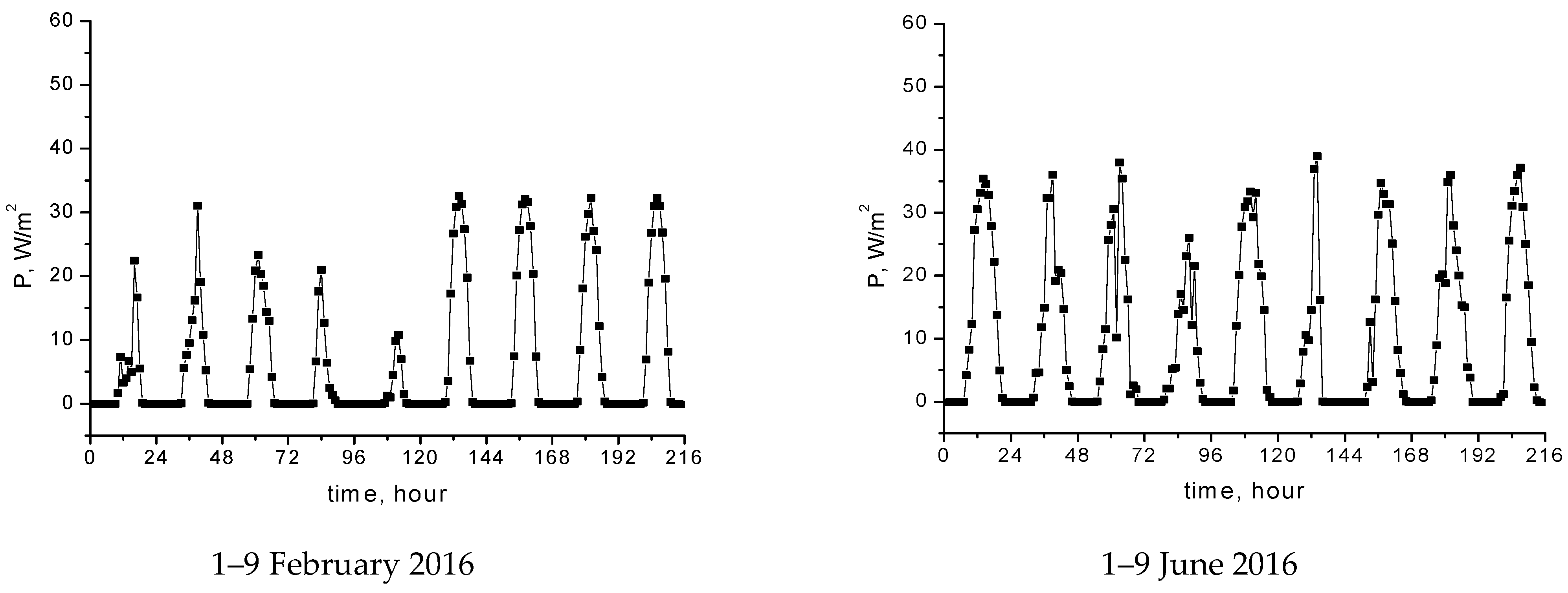
For any statistical analysis, an important aspect is the collection and sampling of the data. In this paper the data are collected from a photovoltaic power plant located in the southeastern part of Romania during the 1 January 2016–31 December 2016 period. The sampled data contain the specific power values for every hour in the given period and these data were used to develop the model. Half of the data accounts for the zero value since the solar irradiance was negligible for 12 h in a day and this is highlighted in the graphs in Figure 1. Hence, the considered time series formed by the hourly data were discontinuous and a new continuous time series was constructed involving the average daily specific power and this was used to predict the average specific power.

A time series was formed with statistical data, collected at regular intervals. A time series represents a sequence of observations on a characteristic measured at successive moments in time or over successive periods. The variable can be measured every hour, day, week, month, or year, or at any other fixed time interval. The model of the data is an important factor in understanding how the time series behaved in the past. If such a demeanor can be expected to continue in the future, the past pattern can be used to select an appropriate prediction method.

From the analysis of the graphs in Figure 1, it follows that the lack of production was higher in winter and lower in summer months, while the maximum specific power delivered was lower in the winter and higher in the summer months.

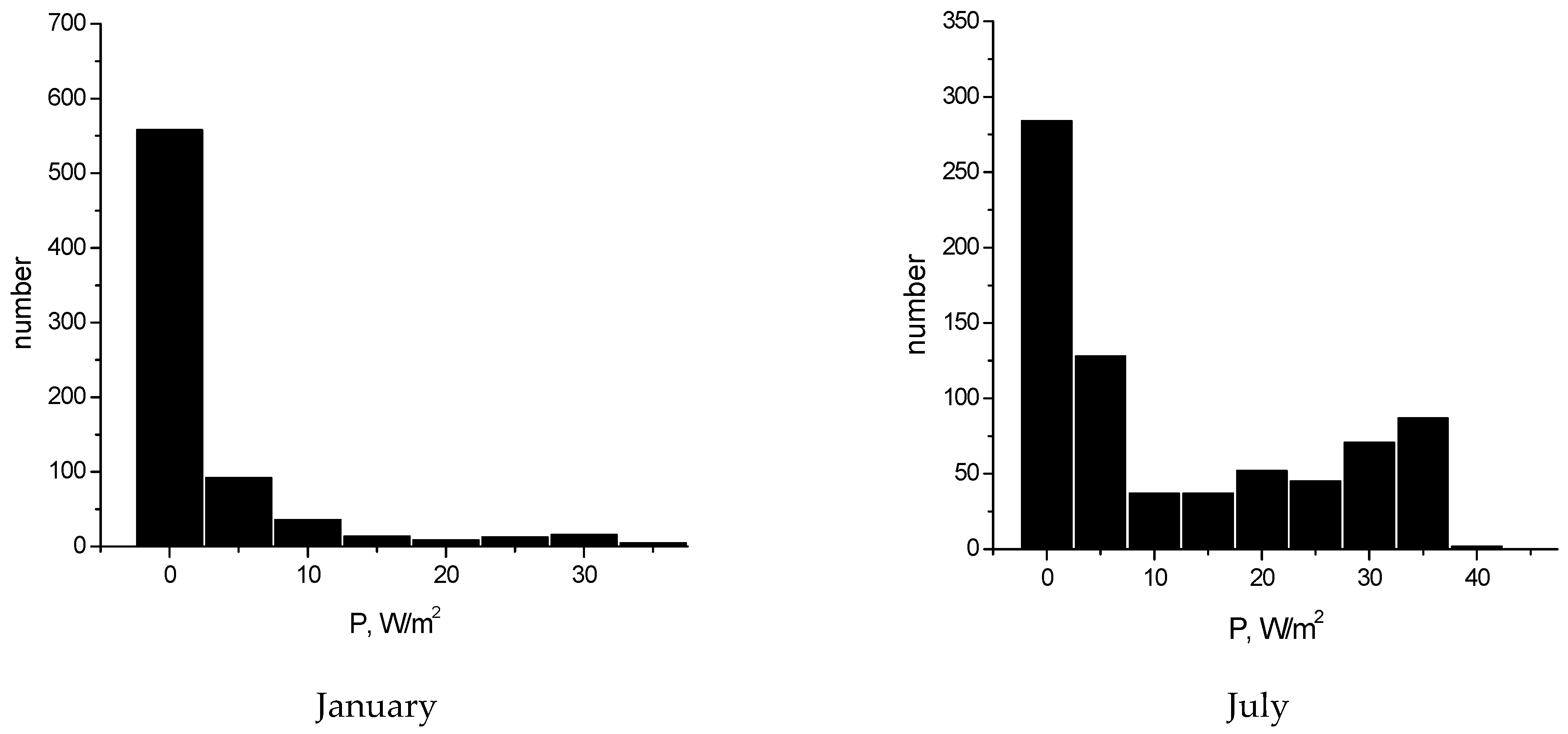
The variation of the circadian cycle overlapped as expected by the variations of the meteorological factors. As a result, the data have a high degree of fluctuation. The same behavior is evidenced by the histograms in Figure 2.

To smooth the past history data, the moving averages provide an efficient and simple method. There are several straightforward moving average methods including simple, double, and weighted moving averages. In all cases, the objective is to smooth past data to estimate the trend cycle component. The moving average describes the procedure of the trend cycle. Each average is computed by dropping the oldest observation and including the next observation.

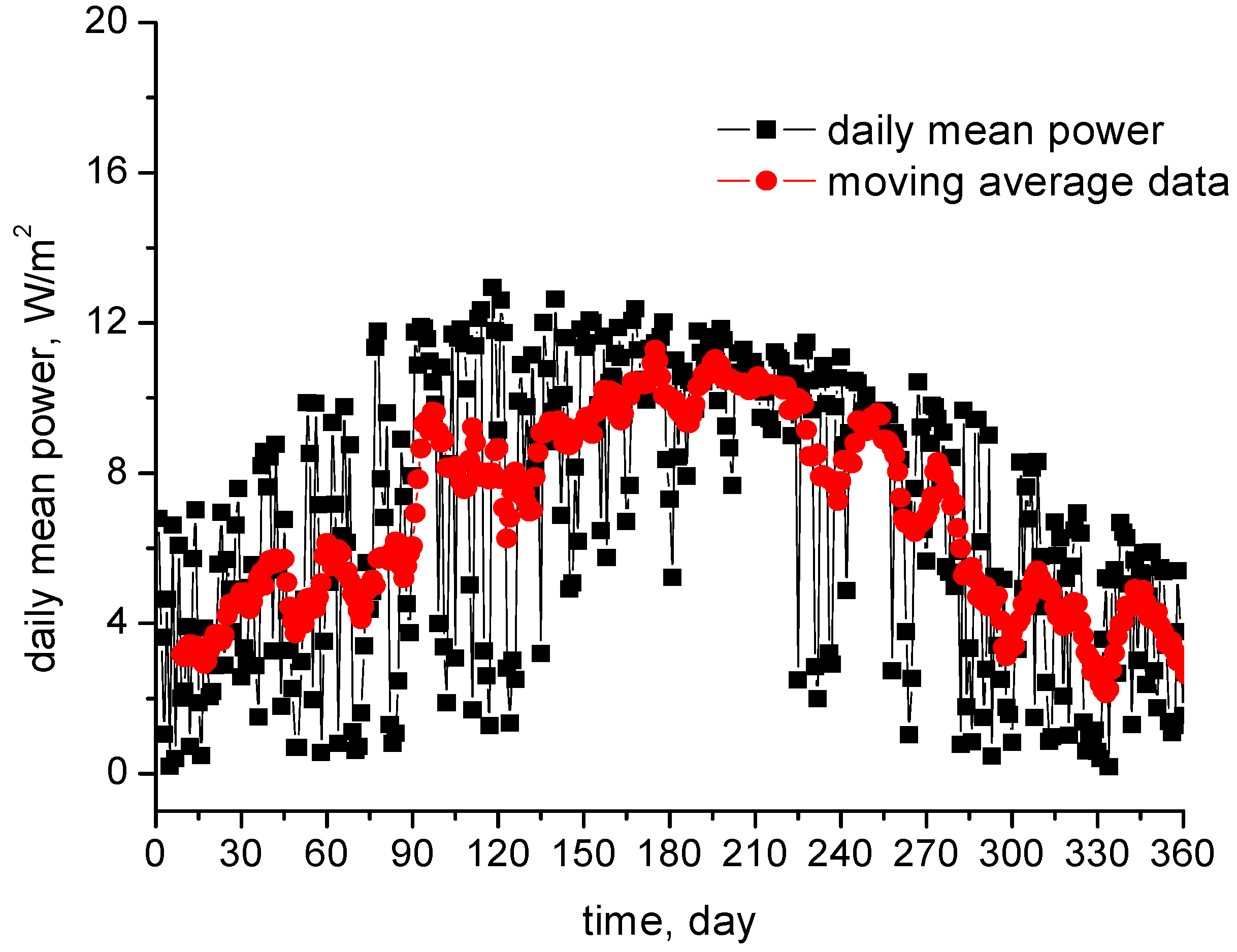
The graph in Figure 3 of the daily average data shows high fluctuations. The attenuation of fluctuations with the moving average (n = 6) highlighted the seasonality of the time series.

The value n = 6 seemed to be optimal for smoothing the data over the entire year. The above graph highlights the fact that the smallest production values were in winter, i.e., at the beginning and at the end of the time interval considered, while the highest amount of power was obtained in summer, in the middle of the data period.

The data from Figure 4 are correlated by nonlinear regression in the following mathematical model (by using the ORIGIN program):

$$y\left(t\right)=6.87+3.38\sin \left[\frac{\pi \left(t-84.79\right)}{177.58}\right].$$

The moving average data from the last figure are those presented in Figure 3 and for these data the above model was obtained.

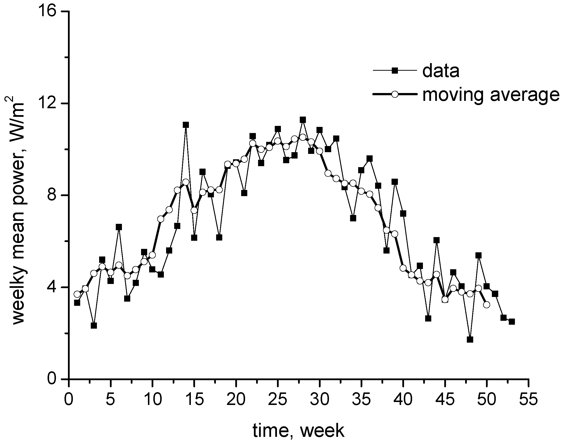
In the following figure, the weekly means of the given data (collected hourly) together with the moving averages of these means were compared. Once again, the seasonality of the moving average data was revealed; at the left and right extremes of the following graph, the small values corresponded to the winter weeks, and larges values were observed in the middle for the summer weeks.

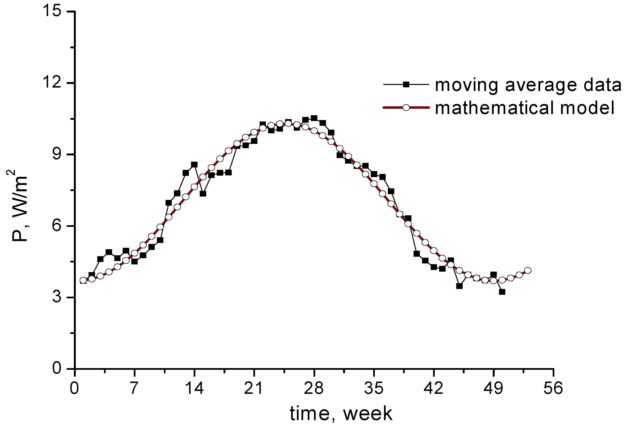
The seasonality was more clearly evidenced if the weekly average data are studied as highlighted by the data from Figure 5 via a moving average with n = 6. Using the ORIGIN program, for the weekly moving average data, the following mathematical model that correlates these data is obtained:

$$y\left(t\right)=7+3.3\sin \left[\frac{\pi \left(t-12.48\right)}{24.34}\right].$$

This last model is consistent with time series as revealed by the graph in Figure 6. The coefficient of determination computed with the same program was R² = 0.90.

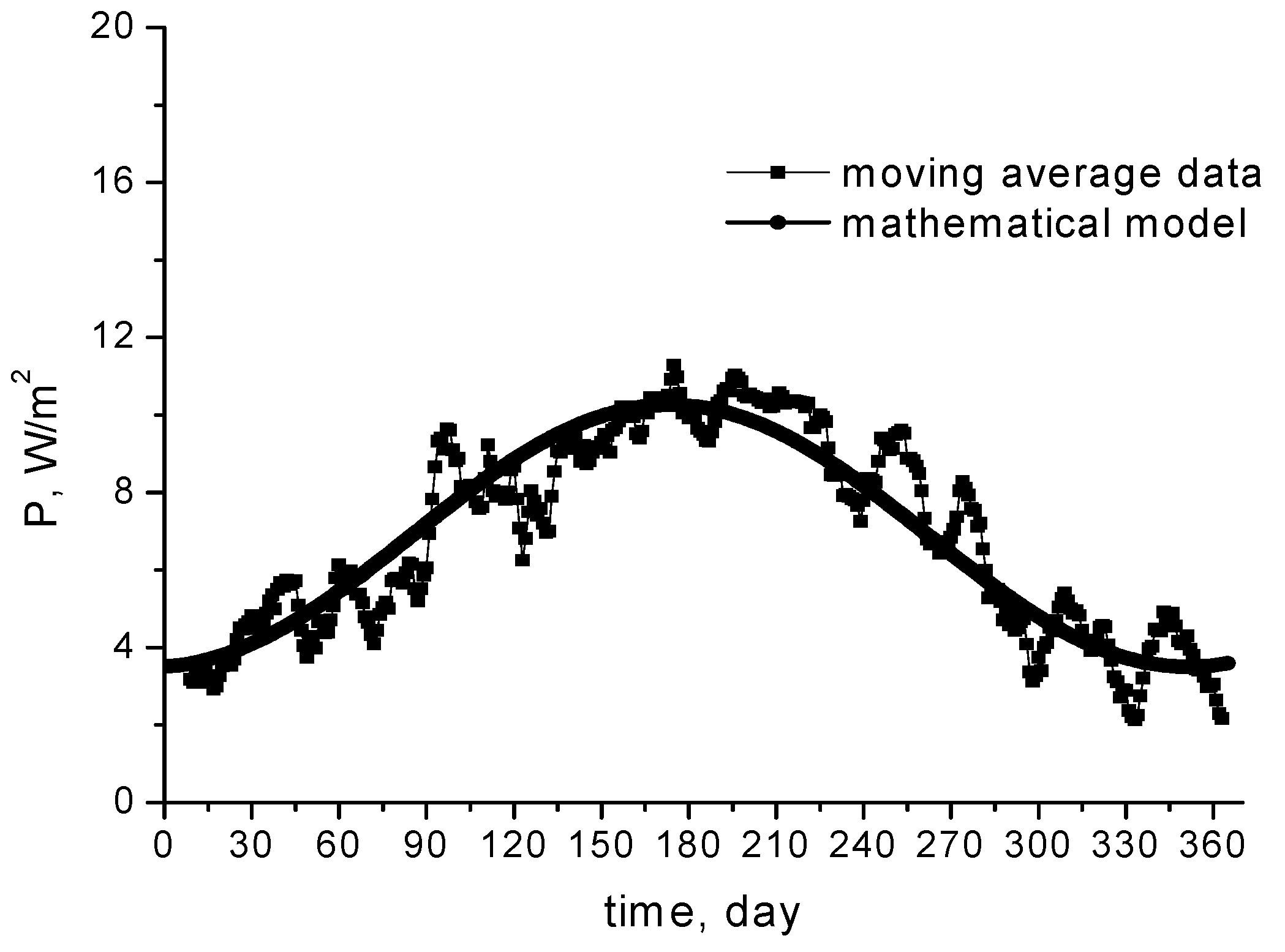
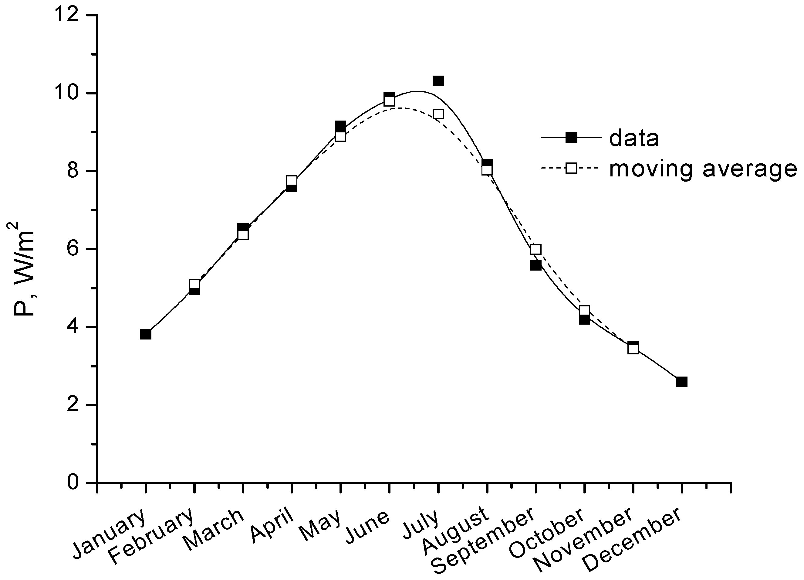
A similar procedure was used for the monthly averages. The monthly means of the collected hourly data were taken and once again the moving average was considered. The resulting graphs are presented in Figure 7, where one can conclude once again that the seasonality produced the low values at the margins which represent the amount of power in winter months, while the production in the summer months was considerably higher.

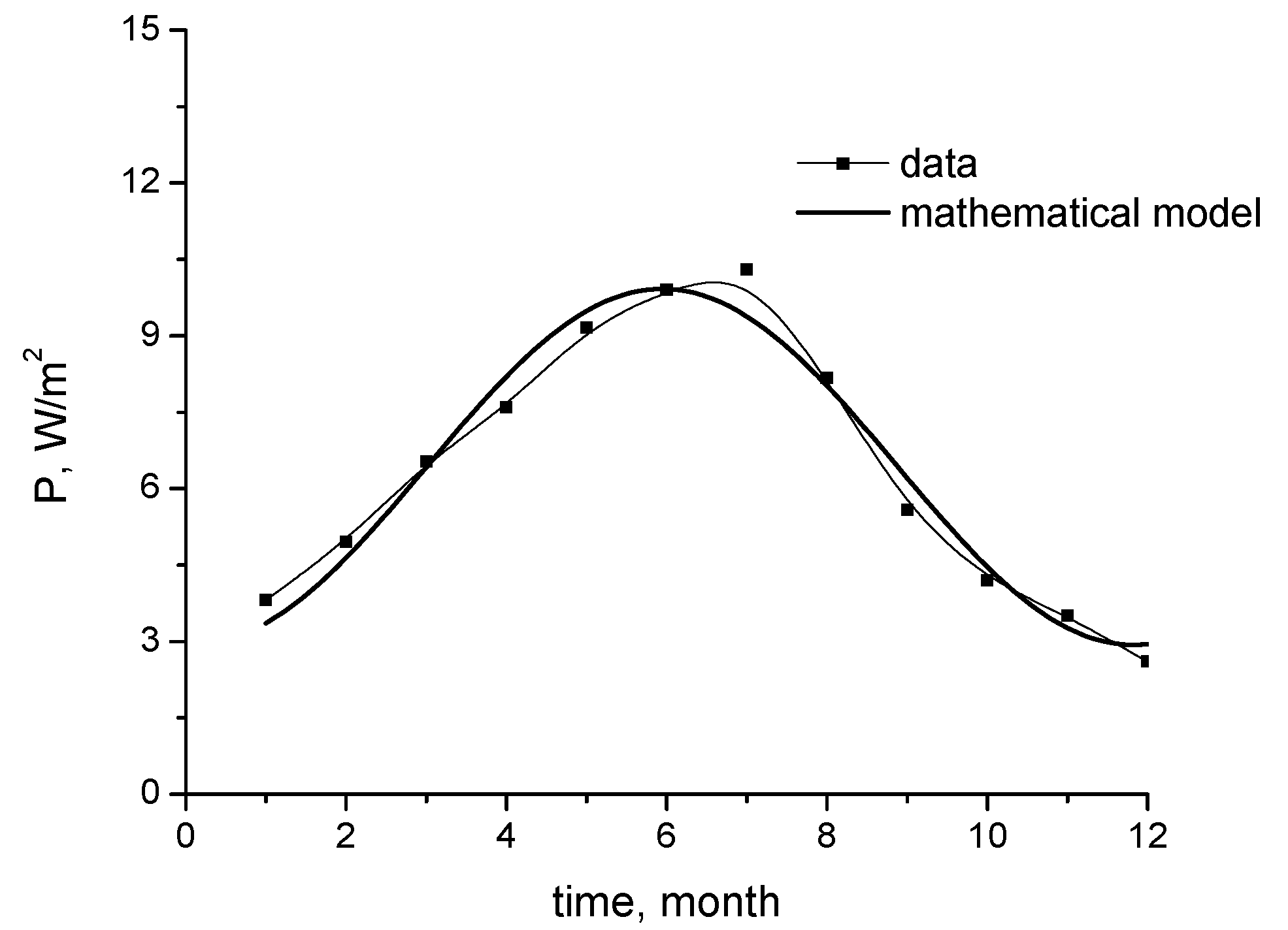
If the same reasoning is applied to the monthly moving average values from Figure 7, the following regression equation (with the coefficient of determination R² = 0.95) was obtained to draw the monthly production:

$$y\left(t\right)=6.4+3.4\sin \left[\frac{\pi \left(t-3\right)}{5.8}\right].$$

The graphical representation of this curve is illustrated in Figure 8 where this mathematical model is superposed over the monthly moving averages.

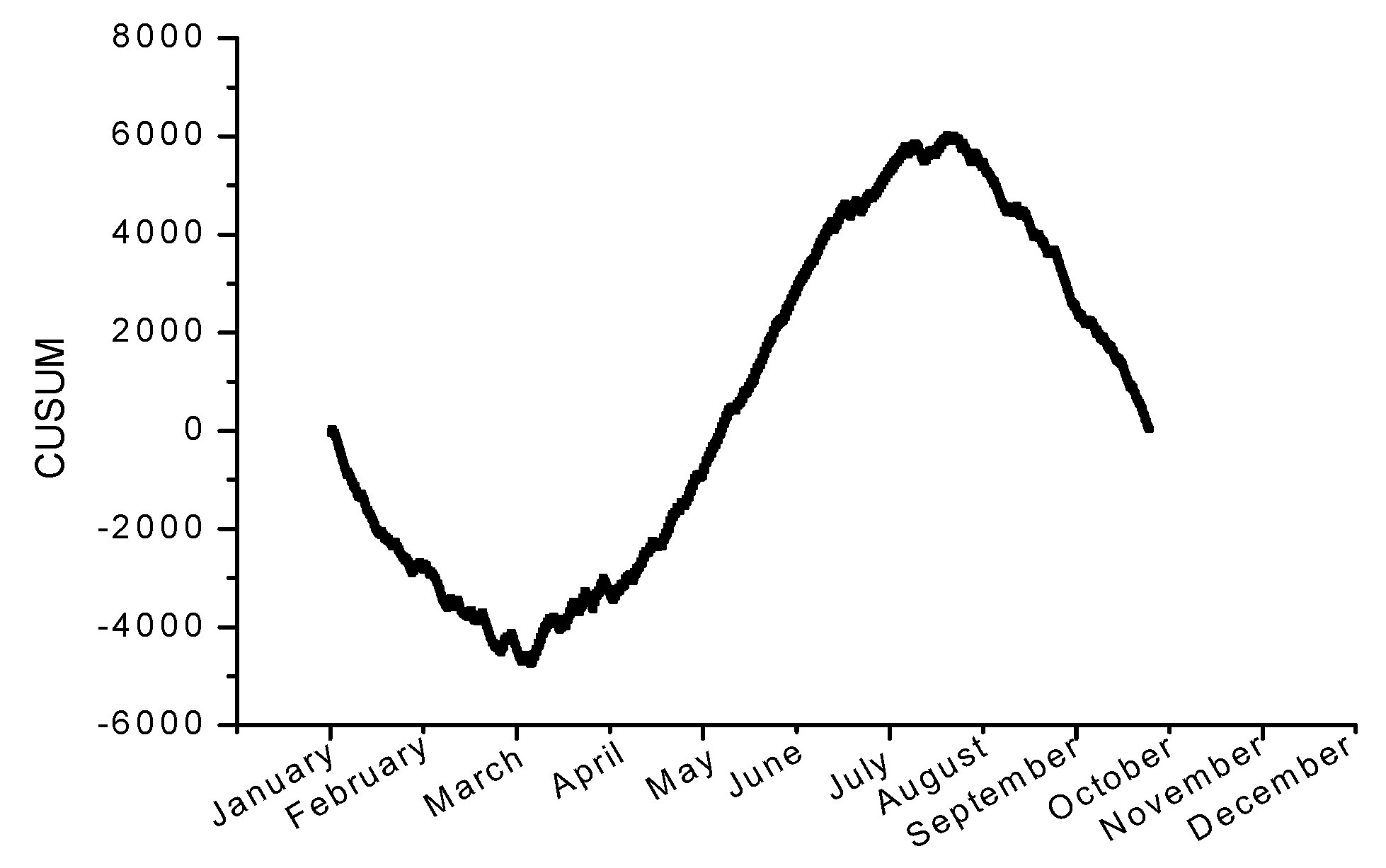
The most sensitive method of trend variation is the CUSUM method. In statistical quality control, the CUSUM chart is used for monitoring changes in trend. The chart from Figure 9 highlights the seasonal character of the original time series data.

The correlation of the data with a linear regression model resulted in a slope of the equation close to zero. It can be deduced that the series was stationary. The same result was obtained if the standard deviation of each seasonality cycle was analyzed.

The statistical analysis of the data revealed that it forms a stationary time series with seasonality.

2.2. Time Series Methods Applied for Eolian Production

The experimental data collected during 2014–2017 from an electric wind power station located in Dobrogea, Romania were analyzed. These data, measured hourly, form a time series. A time series is a set of statistical data, usually collected at regular intervals. As mentioned before, a time series is a sequence of observations on a variable measured at successive points in time or over successive periods of time. The measurements may be taken every hour, day, week, month, or year, or at any other regular interval. The pattern of the data is an important factor in understanding how the time series has behaved in the past. If such behavior can be expected to continue in the future, the past pattern can be used to select an appropriate forecasting method.

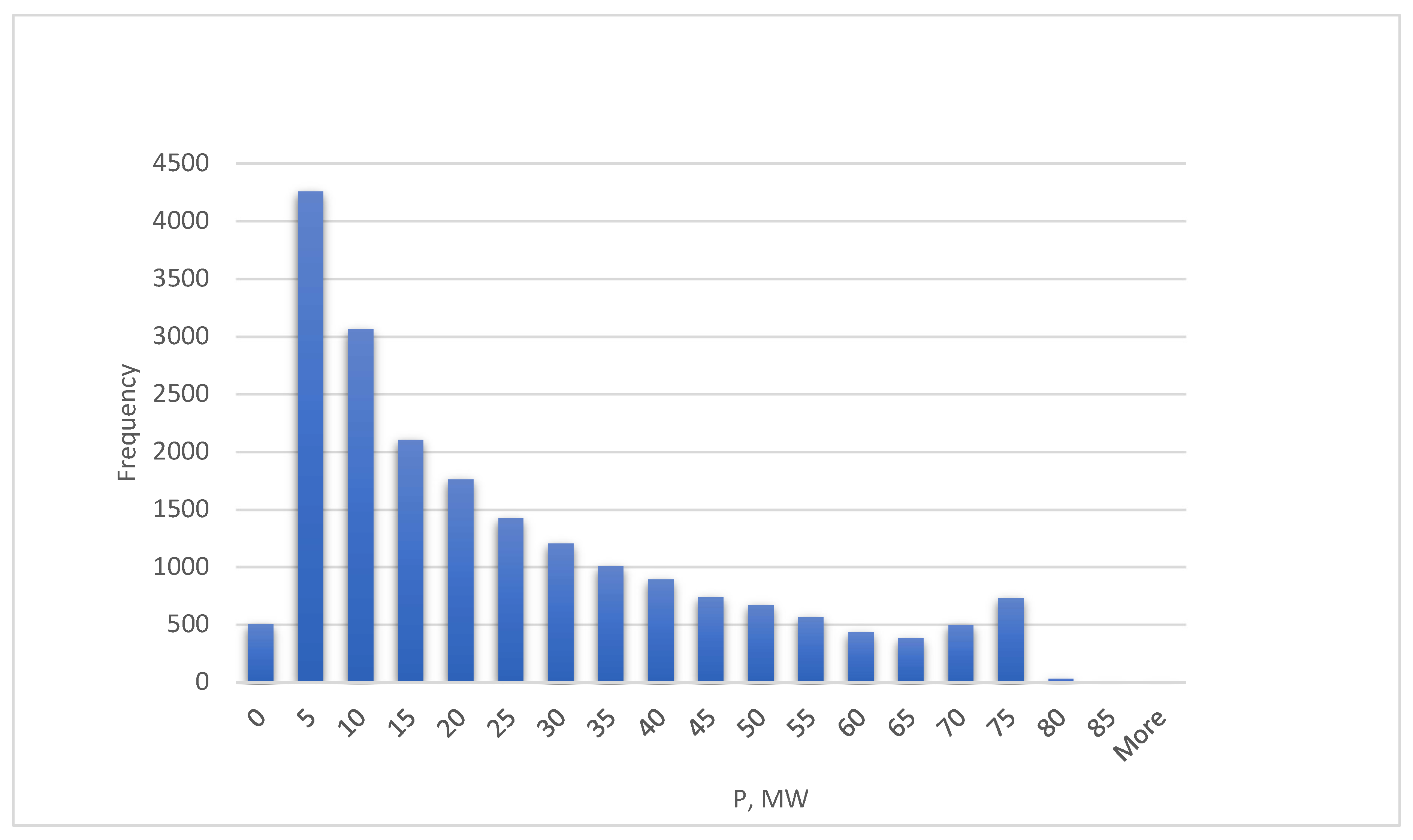
The histogram of these data presented in Figure 10 is asymmetric with a long tail towards positive values. This histogram suggests that the time series has periodic or seasonal properties.

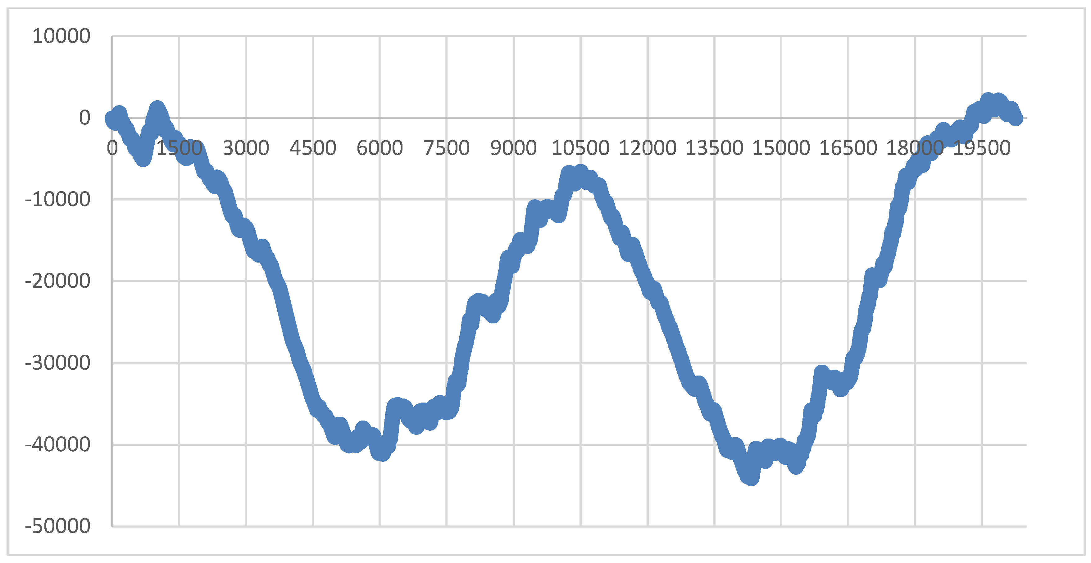
To support this assertion, the CUSUM chart of these data was built since this chart is very sensitive to the trends of the data (Figure 11). The analysis of this chart showed seasonal trend changes. These changes occurred in the months with the highest meteorological instability in the region, namely in April and November, while August is a month of maximal meteorological stability in Romania. At the same time, the small fluctuations of the trend suggest that they may vary with the circadian cycle, either weekly or monthly. In other words, the time scale at which the model is formulated may influence its quality.

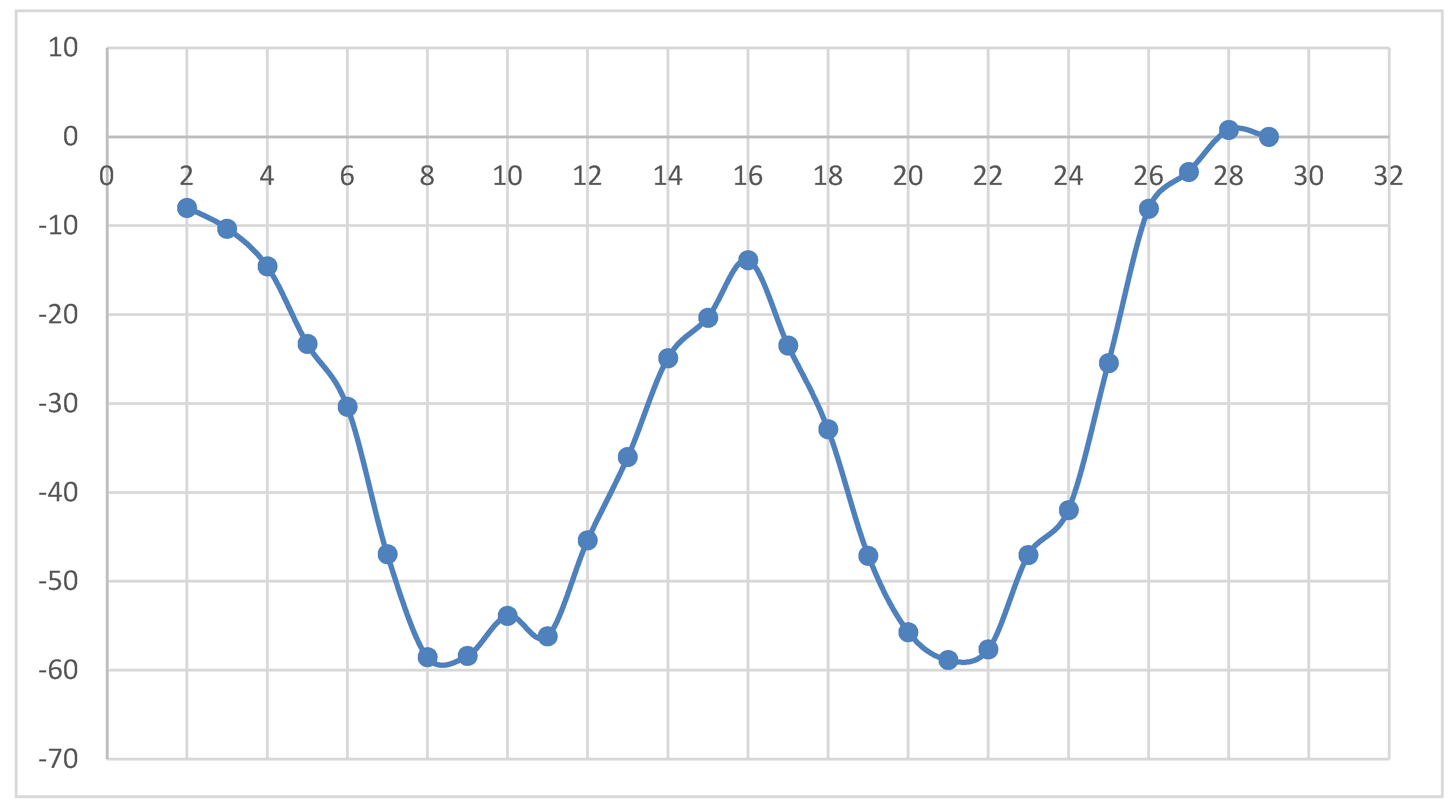
Replacing these data with monthly average values smoothed the fluctuations and better outlined the seasonal trends of the data as shown in Figure 12.

The CUSUM chart is used to monitor the mean of a process based on samples taken from the process at given time points (hours, shifts, days, weeks, months, etc.). The measurements of the samples at a given time constitute a subgroup. Instead of examining the mean of each subgroup independently, the CUSUM chart shows the accumulation of information of current and previous samples.

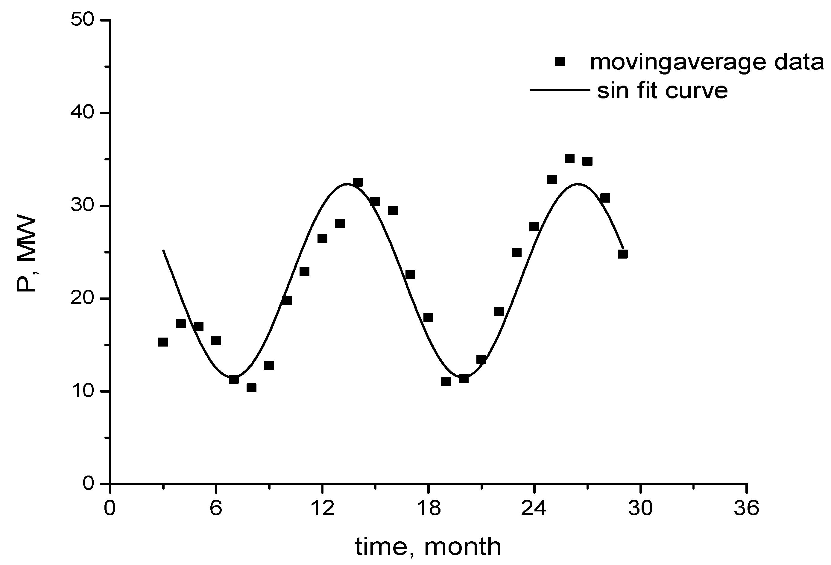
In the figure above, the monthly means treated with moving average are represented together with a proposed mathematical model. The data from Figure 13 were correlated by a nonlinear regression as in the following equation:

$$y\left(t\right)=21.91+10.42\sin \left[\frac{\pi \left(t-10.17\right)}{6.4}\right].$$

Moving averages provide a simple method for smoothing past history data. There are several straightforward moving averages including simple, double, and weighted moving averages. In all cases, the objective is to smooth the past data to estimate the trend of a cycle component. The moving average describes the procedure of trend cycle. Each average is computed by dropping the oldest observation and including the next observation.

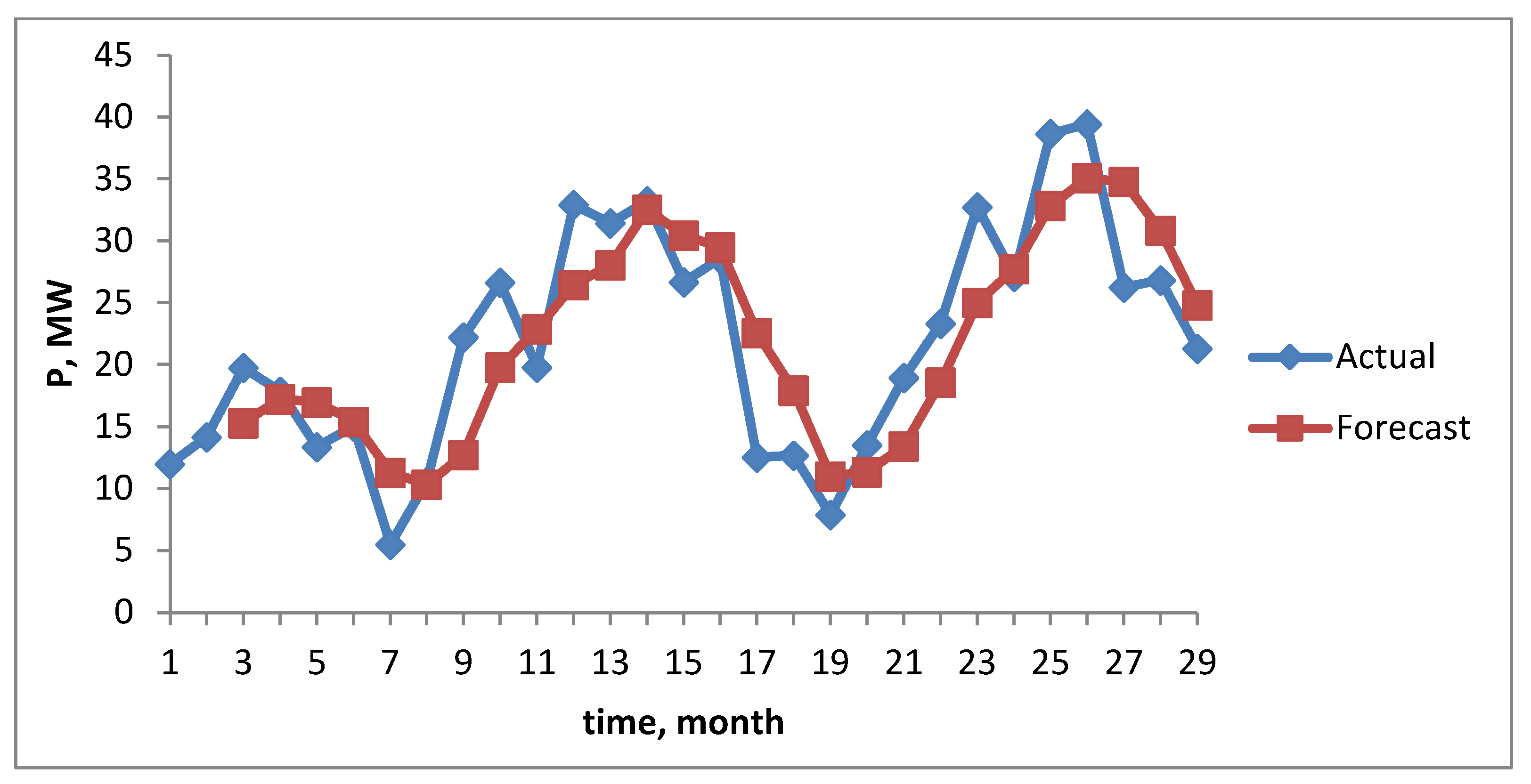
The curves presented in Figure 14 reveal a good agreement between the experimental data (smoothed with moving average) and the statistical model obtained.

3. Results and Discussion

This research first obtained a mathematical model for the power prediction of a photovoltaic plant which is justified by the benefits of this sustainable energy and by the increased production in recent years. At the basis of the study, there is a collection of data representing the hourly power measurements performed during a one-year period. It could be possible to reveal some trends using data over several years, but for this approach we need corresponding information, and this can be the goal of other research. Nevertheless, the seasonal trend established in this study for solar power production seemed to make the analysis of data collected over several years less relevant. In addition, taking into account the fact that the annual solar irradiance presented similar behaviors in different years in the same considered region, and such a statistical approach does not impose a high accuracy, this not being asked for a global evaluation, the analyzed dataset can be considered satisfactory.

Since the collected data form a discontinuous time series, the general properties and procedures cannot be directly applied. For this reason, the moving average (with n = 6) has been used to smooth the data of the analyzed time series in order to obtain mathematical models in good agreement with the experimental data. Since the fluctuations are rather large, many values for n have been tested to obtain the best data smoothing. The value n = 6 was considered the smallest values which could confer the needed smoothness to the time series, and it was sufficiently high to maintain the trend. The time series constructed in this manner are continuous. Prediction models have been developed for the specific power of the next day, next week, and next month. The monthly model was the most accurate, taking into account the superposition of the graphs from Figure 8 and the value of the coefficient of determination. It was proven that the data formed a stationary time series with seasonality by using the CUSUM method.

Similar methods were applied for the second set of data provided from a wind farm. In this case, once again the moving average was used to smooth the data. By using the CUSUM chart of the monthly average data, the seasonal trend of the data was obtained. For the smoothed data, mathematical models of power prediction for the next day, week and month were tested. However, only the model which forecasted the wind power production of the next month was validated. For this reason, the series of results for solar power production could not be extended for obtaining the eolian energy plant production.

Time series data often arise when monitoring a continuous phenomenon involving a huge volume of measurements. The reason for using the properties of time series is to understand the driving forces and structures that produce the observed data and to draw a model for the data to allow for forecasting, monitoring, feedback, and feed forward control. There was a major difference between modeling the data via time series methods and using the process monitoring methods, since in the time series analysis the data points taken over time may have internal structures such as trends or seasonal variations.

The monitored data formed a discontinuous time series. For such a time series, the general theory and its properties do not work. For this reason, by using the moving average to smooth the data of the analyzed time series, some mathematical models in good agreement with the experimental data were obtained.

By comparing the two models for solar and wind production, one can remark that the characterization with time series was more appropriate for the first case. The CUSUM charts clearly revealed the trend and the seasonality in both cases.

For both power productions (solar and eolian) modeling and forecasting, theoretical analyses based on stochastic models of Weibull, Beta, and Rayleigh distributions using probability density function approaches, various statistical indicators such as the determination coefficient (R²), Chi square error (χ²), root mean square error (RMSE), and mean bias error (MBE) are the subject of future works.

The present study was focused on power quantity modeling, forecasting, and prediction in order to integrate renewable energy production into the general energy system. However, the real problem mainly consists of storage issues and marketing/cost analyses. An interesting approach following more targeted branches was made by Pereira and Pereira [60] where, based on the Choquet multi-criteria preference aggregation model, an analysis was performed in order to explore interesting ways which can help governments to make decisions in sustainable energy development.

Compared to the other works cited in the Introduction, there are many studies where the precision was much higher than in the forecast models proposed in this paper. However, we were interested in integrating the production of the considered power plant into the global energy system, so our approximation was sufficient to determine the generation amount. The methods proposed here are simple and easy to be reproduced in similar conditions, taking into account that, for any other situation, a new study related to the new data from the respective station is necessary in order to obtain appropriate forecasting models aiming the global integration.

4. Conclusions

This work corroborated some statistical methods to design the power production of a solar plant and a wind farm in order to obtain some mathematical models to forecast and integrate their production into the general energy system. We considered that for such a global objective, a fairly broad approximation was sufficient, taking into account the simplicity of the proposed procedure and its reproducibility for any other location.

The two collections of data provided from the hourly measurements of the power produced by each plant formed discontinuous time series. The moving average was used to smooth the data of the time series obtained.

The mathematical models proposed were in good agreement with the experimental data. The time series constructed using the moving average were continuous for both data collections. The model developed for solar production could predict the specific power of the next day, next week, and next month and the most accurate model was the monthly model. For the wind farm, only the monthly model showed good concordance with the experimental data.

Using the CUSUM method, we found that the data formed stationary time series with seasonality in both cases, i.e., for photovoltaic and eolian power production.

While there are many studies with quite accurate prediction possibilities superior to those of our models, the advantages of these proposed systems consist in their simplicity and good reproducibility.

Other statistical methods can be used to draw conclusions regarding these two sets of data which represent the subject for other works. However, the results obtained in this study can be considered as the basis for the integration of these renewable energy forms into the national system. Such research can be followed by a complex and thorough analysis of the specific elements which continue the integration process to arrive at a reliable model of sustainable development.

References

- Perma, V.; Uma Rao, K. Development of statistical time series models for solar power prediction. Renew. Energy 2015, 83, 100–109. [Google Scholar] [CrossRef]
- Reikard, G. Predicting solar radiation at high resolutions: A comparison of time series forecasts. Sol. Energy 2009, 83, 342–349. [Google Scholar] [CrossRef]
- Ahmad, A.; Anderson, T.N.; Lie, T.T. Hourly global solar irradiation forecasting for New Zealand. Sol. Energy 2015, 122, 1398–1408. [Google Scholar] [CrossRef] [Green Version]
- Lachhab, S.E.; Bliya, A.; Al Ibrahmi, E.; Dlimi, L. Theoretical analysis, and mathematical modeling of a solar cogeneration system in Morocco. AIMS Energy 2019, 7, 743–759. [Google Scholar] [CrossRef]
- Ngoc, T.N.; Quang, N.N.; Duy, L.B. Reconfiguration of Solar Panels: Mathematical Model and Analysis. Am. J. Electr. Power Energy Syst. 2019, 8, 104–110. [Google Scholar] [CrossRef] [Green Version]
- Amusat, R.O.; Shodyia, S.; Ngadda, Y.H. Mathematical Modeling of Solar Photovoltaic Module to generate Maximum Power Using Matlab/Simulink. IJATR 2021, 2, 1–11. [Google Scholar]
- Das, S.; Samadhiya, A.; Namrata, K. Mathematical Modelling Based Solar PV Module, and its Simulation in comparison with data sheet of JAPG-72-320/4BB Solar Module. In Proceedings of the National Conference on Research and Developments in Material Processing, Modelling and Characterization 2020, Jharkhand, India, 26–27 August 2020. [Google Scholar]
- Jakhrani, A.Q.; Samo, S.R.; Kamboh, S.A.; Labadin, J.; Rigit, A.R.H. An Improved Mathematical Model for Computing Power Output of Solar Photovoltaic Modules. Int. J. Photoenergy 2014, 2014, 346704. [Google Scholar] [CrossRef]
- Sánchez, M.G.; Macia, Y.M.; Gil, A.F.; Castro, C.; Gonzáles, S.N.; Yanes, J.P. A Mathematical Model for the Optimization of Renewable Energy Systems. Mathematics 2021, 9, 39. [Google Scholar] [CrossRef]
- Filho, L.G.; Neto, D.V.; Cremasco, C.; Seraphim, O.; Caneppele, F. Mathematical Analysis of Maximum Power Generated by Photovoltaic Systems and Fitting Curves for Standard Test Conditions. Eng. Agríc. Jaboticabal 2012, 32, 650–662. [Google Scholar] [CrossRef] [Green Version]
- Kadeval, H.N.; Patel, V.K. Mathematical modelling for solar cell, panel and array for photovoltaic system. J. Appl. Nat. Sci. 2021, 13, 937–943. [Google Scholar] [CrossRef]
- Guerra, D.; Iakovleva, E. Mathematical modeling of parameters of solar modules for a solar power plant 2.5 MW in the climatic conditions of the Republic of Cuba. E3S Web Conf. 2019, 140, 04013. [Google Scholar] [CrossRef] [Green Version]
- Premkumar, M.; Kuma, C.; Sowmya, R. Mathematical Modelling of Solar Photovoltaic Cell/Panel/Array Based on the Physical Parameters from the Manufacturer’s Datasheet. Int. J. Renew. Energy Dev. 2020, 9, 7–22. [Google Scholar] [CrossRef]
- Zhu, W.; Wu, B.; Yan, N.; Ma, Z.; Wang, L.; Liu, W.; Xing, Q.; Xu, J. Estimating Sunshine Duration Using Hourly Total Cloud Amount Data from a Geostationary Meteorological Satellite. Atmosphere 2020, 11, 26. [Google Scholar] [CrossRef] [Green Version]
- Haitham, O.; Jamel, M.; Ihab, S. Statistical analysis and mathematical modeling of modified single slope solar still. Energy Sources 2020, 43, 2788–2806. [Google Scholar] [CrossRef]
- Kim, Y.S.; Joo, H.Y.; Kim, J.W.; Jeong, S.Y.; Moon, J.H. Use of a Big Data Analysis in Regression of Solar Power Generation on Meteorological Variables for a Korean Solar Power Plant. Appl. Sci. 2021, 11, 1776. [Google Scholar] [CrossRef]
- Jung, A.-H.; Lee, D.-H.; Kim, J.-Y.; Kim, C.K.; Kim, H.-G.; Lee, Y.-S. Regional Photovoltaic Power Forecasting Using Vector Autoregression Model in South Korea. Energies 2022, 15, 7853. [Google Scholar] [CrossRef]
- Yang, Y.; Yu, T.; Zhao, W.; Zhu, X. Kalman Filter Photovoltaic Power Prediction Model Based on Forecasting Experience. Front. Energy Res. 2021, 9, 682852. [Google Scholar] [CrossRef]
- De Giorgi, M.G.; Congedo, P.M.; Malvoni, M. Photovoltaic power forecasting using statistical methods: Impact of weather data. IET Sci. Meas. Technol. 2014, 8, 90–97. [Google Scholar] [CrossRef]
- Agoua, X.G.; Girard, R.; Kariniotakis, G. Probabilistic Model for Spatio-Temporal Photovoltaic Power Forecasting. IEEE 2019, 10, 780–789. [Google Scholar] [CrossRef] [Green Version]
- Pasari, S.; Nandigama, V.S.S.K. Statistical Modeling of Solar Energy. In Life Cycle Engineering and Management; Sangwan, K.S., Herrmann, C., Eds.; Sustainable Production; Springer: Berlin/Heidelberg, Germany, 2021. [Google Scholar]
- Kam, O.L.; Noël, S.; Ramenah, H.; Kasser, P.; Tanougast, C. Comparative Weibull Distribution Methods for Reliable Global Solar Irradiance Assessment in France Areas; Elsevier: Amsterdam, The Netherlands, 2020; Available online: https://www.elsevier.com/open-access/userlicense/1.0 (accessed on 7 December 2022).
- Bashahu, M.; Ntirandekura, D. Analysis of Sunshine Duration Data Using Two-Parameter Weibull Distributions. Mod. Environ. Sci. Eng. 2019, 5, 635–644. [Google Scholar]
- Zamo, M.; Mestre, O.; Arbogast, P.; Pannekoucke, O. A benchmark of statistical regression methods for short-term forecasting of photovoltaic electricity production, part I: Deterministic forecast of hourly production. Sol. Energy 2014, 105, 792–803. [Google Scholar] [CrossRef]
- Zamo, M.; Mestre, O.; Arbogast, P.; Pannekoucke, O. A benchmark of statistical regression methods for short-term forecasting of photovoltaic electricity production. Part II: Probabilistic forecast of daily production. Sol. Energy 2014, 105, 804–816. [Google Scholar] [CrossRef]
- Yusof Sulaiman, M.; Hlaing Oo, W.M.; Abd Wahab, M.; Zakaria, A. Application of beta distribution model to Malaysian sunshine data. Renew. Energy 1999, 18, 573–579. [Google Scholar] [CrossRef]
- Fentis, A.; Bahatti, L.; Tabaa, M.; Mestari, M. Short-term nonlinear autoregressive photovoltaic power forecasting using statistical learning approaches and in-situ observations. Int. J. Energy Environ. Eng. 2019, 10, 189–206. [Google Scholar] [CrossRef] [Green Version]
- AlKandari, M.; Ahmad, I. Solar power generation forecasting using ensemble approach based on deep learning and statistical methods. Appl. Comput. Inform. 2020. [Google Scholar] [CrossRef]
- Batsala Ya, V.; Hlad, I.V.; Yaremak, I.I.; Kiianiuk, O.I. Mathematical model for forecasting the process of electric power generation by photoelectric stations. Nauk. Visnyk Natsionalnoho Hirnychoho Universytetu 2021, 111–116. [Google Scholar] [CrossRef]
- Chang, W.Y. A literature review of wind forecasting methods. J. Power Energy Eng. 2014, 2, 161–168. [Google Scholar] [CrossRef]
- Wang, X.; Guo, P.; Huang, X. A review of wind power forecasting models. Energy Procedia 2011, 12, 770–778. [Google Scholar] [CrossRef] [Green Version]
- Lange, M.; Focken, U. New developments in wind energy forecasting. In Proceedings of the 2008 IEEE Power and Energy Society General Meeting–Conversion and Delivery of Electrical Energy in the 21st Century, Pittsburgh, PA, USA, 20–24 July 2008. [Google Scholar]
- Giebel, G.; Kariniotakis, G.; Brownsword, R. The State-of-the-Art in Short-Term Prediction of Wind Power—A Literature Review. 2006. Available online: http://www.anemos-project.eu/ (accessed on 7 December 2022).
- Garcia, A.; De-La-Tore-Vega, E. A statistical wind power forecasting system—A Mexican wind farm case study. In Proceedings of the European Wing Energy Conference & Exhibition—EWEC Parc Chanot, Marseille, France, 16–19 March 2009. [Google Scholar]
- Bidaoui, H.; El Abbassi, I.; El Bouardi, A.; Darcherif, A. Wind speed data analysis using Weibull and Rayleigh distribution functions, case study: Five cities Northern Morocco. Procedia Manuf. 2019, 32, 786–793. [Google Scholar] [CrossRef]
- Akpınar, E.K.; Akpınar, S.; Balpetek, N. Statistical analysis of wind speed distribution of Turkey as regional. J. Eng. Technol. Appl. Sci. 2018, 3, 35–55. [Google Scholar] [CrossRef]
- Al Buhairi, M.H. A Statistical analysis of wind speed data and an assessment of wind energy potential in Taiz-Yemen. Ass. Univ. Bull. Environ. Res. 2006, 9, 21–33. [Google Scholar]
- Maina, A.W.; Kamau, J.N.; Timonah, S.; Saoke, C.O.; Nishizawa, Y. Correlation of wind patterns using Weibull and Rayleigh models for St. Xavier secondary school, Naivasha and Jkuat sites. In Proceedings of the The 2015 JKUAT Scientific Conference, Water, Energy, Environment and Climate, Juja, Kenya, 13–16 November 2015; pp. 289–307. [Google Scholar]
- Pobocikova, I.; Sedliackova, Z.; Simon, J. Statistical analysis of wind data based on Weibull and Rayleigh distributions. Communications 2014, 16, 136–141. [Google Scholar] [CrossRef]
- Parajuli, A. A Statistical Analysis of Wind Speed and Power Density Based on Weibull and Rayleigh Models of Jumla, Nepal. Energy Power Eng. 2016, 8, 271–282. [Google Scholar] [CrossRef] [Green Version]
- Mi, A. Wind speed prediction analysis using Rayleigh distribution. Int. J. Stat. Appl. Math. 2020, 5, 24–27. [Google Scholar]
- Arikan, Y.; Arslan, Ö.P.; Çam, E. The analysis of wind data with Rayleigh distribution and optimum turbine and cost analysis in Elmadag, Turkey. IU-JEEE 2015, 15, 1907–1912. [Google Scholar]
- Serag, S.; Ibaaz, K.; Echchelh, A. Statistical study of wind speed variations by Weibull parameters for Socotra Island, Yemen. E3S Web Conf. 2021, 234, 00045. [Google Scholar] [CrossRef]
- Woldegiyorgis, T.A.; Terefe, E.A. Wind Energy potential Estimation Using Weibull and Rayleigh Distribution Models and surface measured data at Debre Birehan, Ethiopia. Appl. J. Envir. Eng. Sci. 2020, 6, 244–262. [Google Scholar]
- Milligan, M.; Schwartz, M.; YWan, Y. Statistical wind power forecasting models: Results for U.S. wind farms. In Proceedings of the WINDPOWER 2003, Austin, TX, USA, 18–21 May 2003. [Google Scholar]
- Islam, K.D.; Chaichana, T.; Dussadee, N.; Intaniwet, A. Statistical distribution and energy estimation of the wind speed at Saint Martin’s Island, Bangladesh. Int. J. Renew. Energy 2017, 12, 77–88. [Google Scholar]
- Zhou, S.; Yang, Y.; Gao, Z.; Xi, X.; Duan, Z.; Li, Y. Estimating vertical wind power density by using tower observation and empirical models over varied desert steppe terrain in northern China. Atmos. Meas. Tech. 2021, 15, 757–773. [Google Scholar] [CrossRef]
- Chiodo, E.; Pio Di Noia, L. Stochastic Extreme Wind Speed Modeling and Bayes Estimation under the Inverse Rayleigh Distribution. Appl. Sci. 2020, 10, 5643. [Google Scholar] [CrossRef]
- Dokur, E.; Ceyhan, S.; Kurban, M. Analysis of Wind Speed Data Using Finsler, Weibull, and Rayleigh Distribution Functions. Electrica 2022, 22, 52–60. [Google Scholar] [CrossRef]
- Barbosa de Alencar, D.; de Mattos Affonso, C.; Limão de Oliveira, L.C.; Moya Rodríguez, J.L.; Cabral Leite, J.; Reston Filho, J.C. Different Models for Forecasting Wind Power Generation: Case Study. Energies 2017, 10, 1976. [Google Scholar] [CrossRef] [Green Version]
- Ekström, J.; Koivisto, M.; Mellin, I.; Millar, R.J.; Lehtonen, M. A Statistical Modeling Methodology for Long-Term Wind Generation and Power Ramp Simulations in New Generation Locations. Energies 2018, 11, 2442. [Google Scholar] [CrossRef] [Green Version]
- Guilizzoni, M.; Eizaguirre, P.M. Trend Lines and Japanese Candlesticks Applied to the Forecasting of Wind Speed Data Series. Forecasting 2022, 4, 165–181. [Google Scholar] [CrossRef]
- Meghea, I.; Mihai, M.; Lăcătuşu, I.; Apostol, T. Time Series Model Applied to Environmental Monitoring Data Analyses. J. Environ. Prot. Ecol. 2012, 13, 426–434. [Google Scholar]
- Meghea, I.; Lăcătuşu, I.; Mihai, M.; Popa, I. Monitoring and Statistics of Athmospheric Pollutant; POLITEHNICA Press: Bucharest, Romania, 2010. [Google Scholar]
- Meghea, I.; Mihai, M.; Lăcătuşu, I.; Iosub, I. Evaluation of Monitoring of Lead Emissions in Bucharest by Statistical Processing. J. Environ. Prot. Ecol. 2012, 13, 746–755. [Google Scholar]
- Meghea, I.; Mihai, M.; Lăcătuşu, I.; Apostol, T. Environmental monitoring of CO emissions: Statistical character of acquired data. Environ. Eng. Manag. J. 2009, 8, 575–582. [Google Scholar] [CrossRef]
- Meghea, I.; Mihai, M.; Crăciun, E. Statistical Control of Mercury in Surface Water of Bucharest. J. Environ. Prot. Ecol. 2012, 13, 1243–1252. [Google Scholar]
- Mihai, M.; Meghea, I. Box-Jenkins methodology applied to the environmental monitoring data. Eng. Appl. Artif. Intell. 2011, 13, 74–81. [Google Scholar]
- Foley, A.M.; Leahy, P.G.; Marvuglia, A.; Mckeogh, E.J. Current methods and advances in forecasting of wind power generation. Renew. Energy 2012, 37, 1–8. [Google Scholar] [CrossRef] [Green Version]
- Pereira, A.A.; Pereira, M.A. Energy storage strategy analysis based on the Choquet multi-criteria preference aggregation model: The Portuguese case. Socio-Econ. Plan. Sci. 2023, 85, 101437. [Google Scholar] [CrossRef]
Figure 1.
The daily production of specific power from solar energy conversion.
Figure 2.
Histograms of specific power distribution data during January and July.
Figure 3.
The attenuation of fluctuations with the moving average (n = 6) of the time series data.
Figure 4.
Relationship between moving average data and the mathematical model.
Figure 5.
The moving average (n = 6) applied to the weekly average data.
Figure 6.
Comparison between weekly moving average data and the mathematical model.
Figure 7.
The moving average (n = 6) applied to the monthly average data.
Figure 8.
Relationship between monthly moving average data and the mathematical model.
Figure 9.
CUSUM chart for original time series data.
Figure 10.
Histogram of the data collected between 2014 and 2017.
Figure 11.
CUSUM chart of data between January 2014 and June 2016.
Figure 12.
CUSUM chart of monthly average data between January 2014 and June 2016.
Figure 13.
Charts of data between January 2014 and June 2016 with monthly average and moving average respectively.
Figure 14.
Correlation between statistical model and data smoothed using moving average method.
Disclaimer/Publisher’s Note: The statements, opinions and data contained in all publications are solely those of the individual author(s) and contributor(s) and not of MDPI and/or the editor(s). MDPI and/or the editor(s) disclaim responsibility for any injury to people or property resulting from any ideas, methods, instructions or products referred to in the content. |
© 2023 by the author. Licensee MDPI, Basel, Switzerland. This article is an open access article distributed under the terms and conditions of the Creative Commons Attribution (CC BY) license (https://creativecommons.org/licenses/by/4.0/).
Share and Cite
MDPI and ACS Style
Meghea, I. Comparison of Statistical Production Models for a Solar and a Wind Power Plant. Mathematics 2023, 11, 1115. https://doi.org/10.3390/math11051115
AMA Style
Meghea I. Comparison of Statistical Production Models for a Solar and a Wind Power Plant. Mathematics. 2023; 11(5):1115. https://doi.org/10.3390/math11051115
Chicago/Turabian StyleMeghea, Irina. 2023. "Comparison of Statistical Production Models for a Solar and a Wind Power Plant" Mathematics 11, no. 5: 1115. https://doi.org/10.3390/math11051115
Note that from the first issue of 2016, this journal uses article numbers instead of page numbers. See further details here.