On Importance of Sensitivity Analysis on an Example of a k-out-of-n System

Abstract

Reliability and sensitivity issues are very close and important problems in any technical system. The system’s sensitivity is understood as the dependence of its behavior on changes in some internal parameters. To perform sensitivity analysis, a general procedure based on a theoretical and numerical study is proposed and applied to a repairable k-out-of-n model. The results show the asymptotic insensitivity of the non-stationary and stationary characteristics of the system reliability to the shape of the repair-time distribution, as well as to the value of its coefficient of variation at a fixed mean. The proposed methodology can be useful to researchers and engineers at the designing stage of real systems, as well as applied to other stochastic reliability models.

1. Introduction

The concept of “sensitivity” has different interpretations depending on the area in which this term is used. This suggests that the so-called sensitivity theory is multidisciplinary (see, for example, [1,2,3]). Despite this, the general meaning of this term is as follows. Sensitivity is understood as some property of a model or a system that is responsible for the variability of the output data by changing its initial parameters. In this paper, sensitivity and its analysis will be considered in the framework of the study of some examples of stochastic systems and processes, which describe their behavior.

Sensitivity analysis (SA) originates from the study of queuing theory models. One of the earliest results concerning the insensitivity of the characteristics of queuing systems to the shape of service time distributions was obtained in 1957 by B. Sevast’yanov. In [4], he proved the insensitivity of the Erlang formulas to the shape of service time distribution with a fixed mean value for loss queuing systems with Poisson input flow.

The theorem proposed and proved by Sevast’yanov served as a starting point in the creation of sensitivity theory within the framework of the queuing theory. Many scientists have made a significant contribution to the development of this theory, i.e., B. Gnedenko, I. Kovalenko, V. Ivnitzkii, V. Kalashnikov, D. Konig, F. Kelly, and others. Furthermore, there are some review articles on this topic (see, for example, [5,6]).

In 1976, I. Kovalenko [7] found the necessary and sufficient conditions for the insensitivity of the stationary reliability characteristics of a redundant renewable system with an exponential lifetime and general distribution of components’ repair time. These conditions consist of a sufficient number of repair units, which means the possibility of immediate restoration of any failed component. The sufficiency of this condition for the case of general distributions of both life and repair time was found in 2013 by V. Rykov [8] with the help of the theory of multidimensional alternative processes. However, these results are invalid in the case of a limited number of repair units for failed components’ restoration.

A significant contribution to the insensitivity study of the stationary state probabilities of various queuing systems and networks, including single-line, multi-line, closed, and open-loop ones, was made by V. Ivnitzkii (see [9,10] for an example). The development of such models has led to the study of systems and networks with several types of demands [11], different types of customers, for example, a network with “negative” customers [12], temporarily non-active customers [13]. On the other hand, the development of Sevast’yanov’s theory led to the study of some generalized semi-Markov processes and their steady-state probabilities’ insensitivity [14,15]. Moreover, there are a number of investigations devoted to SA of some queuing systems and their measures of the service time distribution. The latest research is presented in [16,17,18,19].

In the framework of the sensitivity study of reliability characteristics of stochastic systems, the behavior of systems and processes is often considered in the cases of rare failures or quick recovery. A number of studies on this subject confirm the asymptotic insensitivity of the characteristics of queuing systems to the shape of the repair-time distribution in the case of rare failures or fast recovery [20,21,22].

Any functioning system has many indicators of performance and reliability. In addition, it must be operational for a long time as well as resistant to external or internal factors. Therefore, the reliability study of the system in the context of its stability to the changes in some initial information is a primary task in any applied problem. The purpose of SA, which was discussed above, is to identify the influence of the initial data on the behavior of the whole system. The consequence of this goal may be a set of recommendations for engineers and developers in the context of improving the reliability of the model under study.

This article is devoted to the sensitivity investigation of a repairable k-out-of-n system [23]. Such a system has many applications in management, engineering, telecommunication and many other areas. For example, one of the crucial applications in this area is the reliability study of high-altitude unmanned rotor-craft platforms [24]. The multi-rotor architecture of such a platform allows a platform with n rotary-wing engines to stay operational even after k engines fail. In this paper, it is supposed that a component’s lifetime is exponentially distributed, and repair time is arbitrarily distributed. Within the framework of such a problem statement, time-dependent probabilities, as well as steady-state probabilities of the system, are considered. Although a theoretical study of these characteristics has already been carried out, a numerical analysis, as well as a thorough SA, have not been performed. Since analytical results do not give a complete picture of system behavior, numerical analysis is an integral part of the sensitivity study. The sensitivity of reliability characteristics is investigated not only in the case of rare failures and quick restoration but also in the shape of the repair-time distribution. As an additional parameter for SA, the coefficient of variation, which is defined as the ratio of the standard deviation to the mean, was taken. This indicator is useful in practice since it shows the stability of reliability parameters relative to their average value. Moreover, due to its definition, the coefficient of variation is independent of the unit of measurement.

Currently, there are no clear recommendations in the literature for conducting an SA of stochastic systems. In [2], a general procedure for variance-based SA is presented. Thus, the present article is devoted to filling this gap. The main contribution and novelty of this investigation consist in the following:

-

A general procedure based on well-known research methods in reliability and queuing theories for performing an SA of reliability characteristics of the type of initial information is proposed;

-

The reliability and sensitivity study of a k-out-of-n system is carried out according to the methodology; at the same time, this technique can be applied to other stochastic reliability models;

-

Despite the fact that SAs have already been conducted in the study of k-out-of-n system’s reliability characteristics, novel results of the sensitivity study are obtained.

In the current paper, a modified Kendall’s notation $\langle M_{k<n}\left|GI\right|1\rangle$ to describe the system under consideration is used. Symbols “〈 〉” denote a closed system, i.e., a system with a fixed constant number of unreliable components. M in the first position corresponds to the exponential distribution of a component’s lifetime, $GI$ means (general independent) arbitrary distribution of the components’ repair time. The last position corresponds to the number of repair units.

The paper is organized as follows. Section 2 contains a general procedure for performing an SA, which is applied in further sections. In Section 3, for a k-out-of-n system, some notations, assumptions, and problem settings are established. Section 4 deals with time-dependent system state probabilities for the calculation of which method of supplementary variables [25] is used. In Section 5, the stationary probabilities are presented in the closed form in terms of the Laplace transform of the repair-time distribution. Section 4 and Section 5 are accompanied by numerical and graphical examples for 2-out-of-6 and a 3-out-of-6 systems. Moreover, the steady-state probabilities are considered under both rare failures and quick restoration conditions for the 3-out-of-6 system. The paper ends with a discussion, a conclusion, and some future research directions.

It is important to note that the current article is a continuation of previous research and an extended version of the reports at the 25th International Conference on Distributed Computer and Communication Networks: Control, Computation, Communications (DCCN-2022) (https://dccn.ru/, accessed on 26 January 2023) and the 21st International Conference named after A. Terpugov Information technologies and mathematical modelling (ITMM–2022) (http://itmmconf.ru/, accessed on 26 January 2023). Some analytical results used in the paper were obtained in [21,26]; therefore, some presented theorems contain only the main steps of the proofs with references to already published results.

2. General Procedure for SA Performance

The main contribution of the article consists in drawing up the specific recommendations for conducting SA and proposing an appropriate procedure. As a demonstration of the sensitivity study, a k-out-of-n model is used, and sensitivity of its reliability characteristics to the type of initial information is investigated. The general procedure for SA performance is presented in Figure 1.

Depending on the study being conducted, some steps of this procedure may be in a different sequence or skipped. The implementation of the proposed procedure on an example of a mathematical model of a repairable k-out-of-n system is discussed below in Section 3, Section 4 and Section 5.

3. Problem Setting, Notation, Assumptions

Figure 1 proposes the procedure for performing an SA. The first step is building a mathematical model. Consider a homogeneous repairable k-out-of-n $(1\le k\le n)$ system that has one repair unit. Such a system consists of n components and may be described in two ways, depending on the definition of the parameter k, as follows. The parameter k may represent the number of components in the system that must work in order for the entire system to work, referred to as a k-out-of-n: G system. Or k may represent the number of components in the system that must fail before the entire system fails, referred to as a k-out-of-n: F system. The article will deal with the k-out-of-n: F system, omitting the symbol “F”.

Since both components and the whole system can be restored, many restoration scenarios are possible. This article deals with the following procedure. A failed component is restored at some random time, after which it works again, and other failed components are repaired one-by-one. At that, the order in which the failed components are repaired corresponds to the FCFS (first come first service) model, and the first failed component is restored first. The failure of any k component leads to the system failure and their simultaneous restoration during some random time. After that, the entire system works as a new one. Another scenario of such a system is considered in [27].

Introduce some assumptions about the shape of a component’s life and repair time distributions. Suppose that:

• The lifetimes of system components are independent and exponentially distributed with parameter $\alpha$ and mean time $a={\alpha }^{-1}$;
• According to the system structure, all n components work simultaneously; that is, the system is in a hot redundancy, and therefore, the intensity of one system’s components failure, i.e., when i components of n fail, is

  $${\lambda }_i=(n-i)\alpha ,i=\overline{0,k-1};$$
• The repair times for any failed components are independently identically distributed (i.i.d.) random variables (r.v.’s) $B_i(i=1,2,\cdots )$ with common cumulative distribution function (c.d.f.) $B\left(x\right)=\mathbb{P}\{B_i\le x\}$ which is absolutely continuous, and the probability density function (p.d.f.) is $b\left(x\right)$;
• The repair times for a failed system are also i.i.d. r.v. $F_i(i=1,2,\cdots )$ and their corresponding c.d.f. is $F\left(x\right)=\mathbb{P}\{F_i\le x\}$ and p.d.f. is $f\left(x\right)$;
• The instantaneous repairs are impossible, and their mean times are finite,

  $$B\left(0\right)=F\left(0\right)=0,b=\underset{0}{\overset{\infty }{\int }}(1-B\left(x\right))dx<\infty ,f=\underset{0}{\overset{\infty }{\int }}(1-F\left(x\right))dx<\infty ;$$
• Corresponding Laplace transforms (LTs) of p.d.f.’s $b\left(t\right)$ and $f\left(t\right)$ are

  $$\tilde{b}\left(s\right)=\underset{0}{\overset{\infty }{\int }}{e}^{-st}b\left(t\right)dt,\tilde{f}\left(s\right)=\underset{0}{\overset{\infty }{\int }}{e}^{-st}f\left(t\right)dt.$$

The state space of the system is denoted by $E=\{0,1,2,\cdots ,k-1,k\}$, where

• 0 means that all the components are working; not one is repaired,
• i means that i components out of $n(1\le i\le k-1)$ fail; one of them is repaired with r.v. B, and others $(n-i)$ operate,
• k means full system failure and its repair with r.v. F, after which the system becomes a new one.

To perform a reliability analysis, describe the system behavior as a random process $J=\left\{J\right(t),t\ge 0\}$ on the space set E:

$$J\left(t\right)=j,j\in E,\mathrm{if}\mathrm{the}\mathrm{system}\mathrm{is}\mathrm{in}\mathrm{state}j\mathrm{in}\mathrm{time}t.$$

Suppose that $J\left(0\right)=0$.

In this paper, we consider the calculation of time-dependent system state probabilities (t.d.s.s.p.’s)

$${\pi }_j\left(t\right)=\mathbb{P}\{J\left(t\right)=j\},j\in E,$$

steady-state probabilities (s.s.p.’s)

$${\pi }_j=\underset{t\to \infty }{lim}\mathbb{P}\{J\left(t\right)=j\},j\in E,$$

availability coefficient

$$K_{av}=\sum _{0\le i\le k-1}{\pi }_i=1-{\pi }_k,$$

as well as consider the properties of their asymptotic insensitivity to the shapes of system component’s repair time distributions, including the case of rare failures and quick restoration.

4. Time-Dependent System State Probabilities

4.1. Markovization Method

The second step in SA calculates t.d.s.s.p.’s of the $\langle M_{k<n}\left|GI\right|1\rangle$ system. For this, the method of supplementary variables (one of the Markovization methods) is proposed. This method was firstly introduced by Cox and traditionally used in studies of various stochastic systems. In our case, as a supplementary variable, consider the elapsed repair time of a failed component or a failed system. Thus, denote by

$$Z\left(t\right)={\{J\left(t\right),X\left(t\right)\}}_{t\ge 0}$$

a two-dimensional process, where $J\left(t\right)$ is defined as above, and $X\left(t\right)$ means the elapsed repair time of the failed component or the whole system failure. Due to the method used, the process $Z\left(t\right)$ is a Markov one with discrete-continuous states space $\overline{E}=\{0,(i,x)\mid i=\overline{1,k},x\in {\mathbb{R}}_{+}\}$, where

• 0 means that there is no failed component, all the components are working,
• $(i,x),i=\overline{1,k}$ means that i components have failed and the elapsed repair time of the failed component or the whole system failure equals x;
• $(1,0)$ means that one of the system’s components has failed, after which its repair immediately begins; or one of the two failed elements has been repaired, its elapsed recovery time is reset to zero, after which repair of the second failed component immediately begins;
• $(i,0)$ means that from $i,i=\overline{2,k-1}$ failed components, one has been repaired, after which the corresponding repair time is reset to zero and repair of the other failed component immediately begins;
• $(k,0)$ means that the k-th failure has occurred (failure of the k-th component), after which the repair of one and the failed component stops, and restoration of all failed elements begins simultaneously.

Denote the t.d.s.s.p.’s of the process $Z\left(t\right)$,

• ${\pi }_0\left(t\right)=\mathbb{P}\{J\left(t\right)=0\}$—the probability of a working state of all system components at time t;
• ${\pi }_i(t;x)dx=\mathbb{P}\{J\left(t\right)=i;x<X\left(t\right)\le x+dx\}$—the joint probability that at time t there are i failed components, among which one is repaired with the elapsed repair time in the interval x and $x+dx$, $i=\overline{1,k}$. Remember that with $i=k$, there is a simultaneous restoration of all failed components.

Further calculations will be based on the following events and the corresponding probabilities.

• The probability that during time $\Delta$ one of the system’s component will fail, provided that it has worked x units of time, is equal to

  $$\begin{array}{ccc}\hfill \mathbb{P}\{x\le A<x+\Delta \mid A\ge x\}={\displaystyle \frac{\mathbb{P}\{x\le A<x+\Delta \}}{\mathbb{P}\{A\ge x\}}}& =& \hfill \\ \hfill ={\displaystyle \frac{A(x+\Delta )-A\left(x\right)}{1-\mathbb{P}\{x<A\}}}={\displaystyle \frac{a\left(x\right)\Delta +o(\Delta )}{1-A\left(x\right)}}={\displaystyle \frac{\alpha e^{-\alpha x}\Delta +o(\Delta )}{e^{-\alpha x}}}& =& \alpha \Delta +o(\Delta ).\hfill \end{array}$$

  (1)
• The probability that starting from the considered moment in time $\Delta$, one of the system’s components will be repaired, provided that it was repaired x amount of times, is

  $$\begin{array}{ccc}\hfill \mathbb{P}\{x\le B<x+\Delta \mid B\ge x\}={\displaystyle \frac{\mathbb{P}\{x\le B<x+\Delta \}}{\mathbb{P}\{B\ge x\}}}& =& \hfill \\ \hfill ={\displaystyle \frac{B(x+\Delta )-B\left(x\right)}{1-\mathbb{P}\{x<B\}}}={\displaystyle \frac{b\left(x\right)\Delta +o(\Delta )}{1-B\left(x\right)}}& =& \beta \left(x\right)\Delta +o(\Delta ).\hfill \end{array}$$

  (2)
• The probability that starting from the considered moment in time $\Delta$, the system will be repaired, provided that its failed element was under repair x amount of times, is

  $$\begin{array}{ccc}\hfill \mathbb{P}\{x\le F<x+\Delta \mid F\ge x\}={\displaystyle \frac{\mathbb{P}\{x\le F<x+\Delta \}}{\mathbb{P}\{F\ge x\}}}& =& \hfill \\ \hfill ={\displaystyle \frac{F(x+\Delta )-F\left(x\right)}{1-\mathbb{P}\{x<F\}}}={\displaystyle \frac{f\left(x\right)\Delta +o(\Delta )}{1-F\left(x\right)}}& =& \varphi \left(x\right)\Delta +o(\Delta ).\hfill \end{array}$$

  (3)

Thus, the corresponding transition graph is shown in Figure 2. Here, the description of the instant start of the repair after the completion of the previous one (from the description of states space $\overline{E}$) corresponds to the transitions from states $(i,0)$ to $(i,x)$, $i=\overline{1,k-2},k$. Moreover, $\beta \left(x\right)=\frac{b\left(x\right)}{1-B\left(x\right)}$ and $\varphi \left(x\right)=\frac{f\left(x\right)}{1-F\left(x\right)}$ are conditional components’ and system’s repair densities, given elapsed repair time x, respectively.

Based on the presented transition graph and using the description of probabilities (1)–(3), one can compose a system of Kolmogorov forward partial differential equations for the t.d.s.s.p.’s calculation.

Theorem 1.

T.d.s.s.p.’s of the process $Z\left(t\right)$ are followed from the system of Kolmogorov forward partial differential equations,

$$\begin{array}{cc}\hfill & {\displaystyle \frac{d}{dt}}{\pi }_0\left(t\right)=-{\lambda }_0{\pi }_0\left(t\right)+{\int }_0^t\beta \left(x\right){\pi }_1(t,x)dx+{\int }_0^t\varphi \left(x\right){\pi }_k(t,x)dx,\hfill \\ \hfill & \left({\displaystyle \frac{\partial }{\partial t}}+{\displaystyle \frac{\partial }{\partial x}}\right){\pi }_1(t,x)=-({\lambda }_1+\beta \left(x\right)){\pi }_1(t,x),\hfill \\ \hfill & \left({\displaystyle \frac{\partial }{\partial t}}+{\displaystyle \frac{\partial }{\partial x}}\right){\pi }_i(t,x)=-({\lambda }_i+\beta \left(x\right)){\pi }_i(t,x)+{\lambda }_{i-1}{\pi }_{i-1}(t,x),i=\overline{2,k-1},\hfill \\ \hfill & \left({\displaystyle \frac{\partial }{\partial t}}+{\displaystyle \frac{\partial }{\partial x}}\right){\pi }_k(t,x)=-\varphi \left(x\right){\pi }_k(t,x),\hfill \end{array}$$

(4)

jointly with the initial

$$\begin{array}{c}\hfill {\pi }_0\left(0\right)=1,{\pi }_i(0;x)=0,i=\overline{1,k},\forall x\ge 0,\end{array}$$

(5)

and boundary conditions

$$\begin{array}{cc}\hfill {\pi }_1(t,0)& ={\lambda }_0{\pi }_0\left(t\right)+{\int }_0^t\beta \left(x\right){\pi }_2(t,x)dx,\hfill \\ \hfill {\pi }_i(t,0)& ={\int }_0^t\beta \left(x\right){\pi }_{i+1}(t,x)dx,i=\overline{2,k-2},\hfill \\ \hfill {\pi }_{k-1}(t,0)& =0,\hfill \\ \hfill {\pi }_k(t,0)& ={\lambda }_{k-1}{\pi }_{k-1}\left(t\right).\hfill \end{array}$$

(6)

Proof. 

The general idea of the proof is as follows. The obtained system of differential Equations (4) is based on the construction of the system of finite difference equations by the usual method of comparison of the corresponding process state probability changes on infinitesimal small-time epochs t and $t+\Delta t$.

$$\begin{array}{ccc}\hfill {\pi }_0(t+\Delta )& =& \mathbb{P}\{J(t+\Delta )=0\}=(1-{\lambda }_0\Delta ){\pi }_0\left(t\right)+{\int }_0^t\beta \left(x\right)dx{\pi }_1(t,x)\Delta +{\int }_0^t\varphi \left(x\right)dx{\pi }_k(t,x)\Delta +o(\Delta ),\hfill \\ \hfill {\pi }_1(t+\Delta ,x+\Delta )dx& =& \mathbb{P}\{J(t+\Delta )=1;x+\Delta <X(t+\Delta )<x+\Delta +dx\}=(1-{\lambda }_1\Delta )(1-\beta \left(x\right)\Delta ){\pi }_1(t,x)+o(\Delta ),\hfill \\ \hfill {\pi }_i(t+\Delta ,x+\Delta )dx& =& \mathbb{P}\left\{J\right(t+\Delta )=i;x+\Delta <X(t+\Delta )<x+\Delta +dx\}=\hfill \\ & =& (1-{\lambda }_i\Delta )(1-\beta \left(x\right)\Delta ){\pi }_i(t,x)+{\lambda }_{i-1}{\pi }_{i-1}(t,x)\Delta +o(\Delta ),i=\overline{2,k-1},\hfill \\ \hfill {\pi }_k(t+\Delta ,x+\Delta )dx& =& \mathbb{P}\{J(t+\Delta )=k;x+\Delta <X(t+\Delta )<x+\Delta +dx\}={\lambda }_{k-1}\Delta {\pi }_{k-1}(t,x)+(1-\beta \left(x\right)\Delta ){\pi }_k(t,x)+o(\Delta ).\hfill \end{array}$$

Then, transforming these expressions and passing then to the limit $\Delta t\to 0$, we obtain the system of differential Equation (4).

The initial conditions (5) follow from the assumption that, at the beginning of the system operation, all its components are operational.

Similarly, by comparing the probabilities of the process states between t and $t+\Delta$, when the additional variable takes values close to zero, we obtain the first two and the last boundary conditions from (6),

$$\begin{array}{ccc}\hfill {\pi }_1(t+\Delta ,\Delta )dx& =& {\lambda }_0{\pi }_0\left(t\right)\Delta +{\int }_0^t\beta \left(x\right)dx{\pi }_2(t,x)\Delta +o(\Delta ),\hfill \\ \hfill {\pi }_i(t+\Delta ,\Delta )dx& =& {\int }_0^t\beta \left(x\right)dx{\pi }_{i+1}(t,x)\Delta ,i=\overline{2,k-1},\hfill \\ \hfill {\pi }_k(t+\Delta ,\Delta )dx& =& {\lambda }_{k-1}{\int }_0^{\infty }{\pi }_{k-1}(t,x)\Delta dx+o(\Delta ).\hfill \end{array}$$

An additional boundary condition for the probability ${\pi }_{k-1}(t,0)$ from (6) follows from the fact that the process $Z\left(t\right)$ is never in the state $k-1$ with elapsed recovery time equal to zero (see Figure 2). □

The algorithm of the solution of the systems (4)–(6) can be found in [26], where the method of characteristics was proposed. In [28], the calculation of t.d.s.s.p.’s of the same model is presented with the help of the theory of decomposable semi-regenerative processes (DSRP). These methods made it possible to obtain t.d.s.s.p.’s in terms of LT of repair time.

Using the obtained results for a 2-out-of-n system, consider some numerical examples to show the insensitivity of their time-dependent characteristics to the shape of the repair time-distribution and its coefficient of variation.

4.2. Numerical Example, Sensitivity

The solution methods mentioned above make it quite easy to obtain non-stationary characteristics of the process in terms of the LT of repair time. However, calculating the inverse LT of a complex function is not a trivial task, even for many mathematical software products. Consider the example below, which does not require large computational efforts to calculate the time-dependent characteristics of a k-out-of-n system. The issue of computational implementation of the inverse LT is not raised, and readers are invited to consider it on their own.

Consider as an example a 2-out-of-n system. Its t.d.s.s.p.’s in terms of the LT of repair time are

$$\begin{array}{ccc}\hfill {\tilde{\pi }}_0\left(s\right)& =& {\displaystyle \frac{s+{\lambda }_1}{s(s+{\lambda }_1)+{\lambda }_0(1-\tilde{b}(s+{\lambda }_1))(s+{\lambda }_1(1-\tilde{f}\left(s\right)))}},\hfill \\ \hfill {\tilde{\pi }}_1\left(s\right)& =& {\displaystyle \frac{{\lambda }_0(1-\tilde{b}(s+{\lambda }_1))}{s(s+{\lambda }_1)+{\lambda }_0(1-\tilde{b}(s+{\lambda }_1))(s+{\lambda }_1(1-\tilde{f}\left(s\right)))}},\hfill \\ \hfill {\tilde{\pi }}_2\left(s\right)& =& \frac{1}{s}·{\displaystyle \frac{{\lambda }_0{\lambda }_1(1-\tilde{b}(s+{\lambda }_1))(1-\tilde{f}\left(s\right))}{s(s+{\lambda }_1)+{\lambda }_0(1-\tilde{b}(s+{\lambda }_1))(s+{\lambda }_1(1-\tilde{f}\left(s\right)))}}.\hfill \end{array}$$

Note, if the repair time of the components and a system is exponentially ($Exp$) distributed, the following remark holds.

Remark 1.

If $B\left(t\right)\sim Exp\left(b^{-1}\right)$ and $F\left(t\right)\sim Exp\left(f^{-1}\right)$, the t.d.s.s.p.’s have the following form,

$$\begin{array}{cc}\hfill {\tilde{\pi }}_0\left(s\right)& ={\displaystyle \frac{(1+fs)(1+b(s+{\lambda }_1))}{s(1+fs)(1+b(s+{\lambda }_0))+bs(1+f(s+{\lambda }_0))}},\hfill \\ \hfill {\tilde{\pi }}_1\left(s\right)& ={\displaystyle \frac{b{\lambda }_0(1+fs)}{s(1+fs)(1+b(s+{\lambda }_0))+bs(1+f(s+{\lambda }_0))}},\hfill \\ \hfill {\tilde{\pi }}_2\left(s\right)& ={\displaystyle \frac{bf{\lambda }_0{\lambda }_1}{s(1+fs)(1+b(s+{\lambda }_0))+bs(1+f(s+{\lambda }_0))}}.\hfill \end{array}$$

(7)

This result coincides with that obtained with the construction of a simple birth and death process, which is described by the following system of Kolmogorov differential equations,

$$\begin{array}{ccc}\hfill \frac{d}{dt}{\pi }_0\left(t\right)& =& -{\lambda }_0{\pi }_0\left(t\right)+b^{-1}{\pi }_1\left(t\right)+f^{-1}{\pi }_2\left(t\right),\hfill \\ \hfill \frac{d}{dt}{\pi }_1\left(t\right)& =& -({\lambda }_1+b^{-1}){\pi }_1\left(t\right)+{\lambda }_0{\pi }_0\left(t\right),\hfill \\ \hfill \frac{d}{dt}{\pi }_2\left(t\right)& =& -f^{-1}{\pi }_2\left(t\right)+{\lambda }_1{\pi }_1\left(t\right).\hfill \end{array}$$

For the third step of SA, determine the model’s parameters as well as the repair time distribution and its coefficient of variation. Suppose that $n=6$. An example of a 2-out-of-6 model corresponds to a mathematical model of high-altitude telecommunication platforms based on tethered unmanned aerial vehicles [24].

Let mean lifetime $a=1$, and the repair time has an Erlang distribution ($Erl(l,\theta )$) with p.d.f. $f\left(t\right)={\displaystyle \frac{{\theta }^l}{\Gamma \left(l\right)}}{t}^{l-1}{e}^{-\theta t},t>0$. Corresponding means are b and f, and coefficients of variation are $v_b$ and $v_f$. During this section, indexes b and f are denoted parameters of components’ and system’s repair times, respectively, as well as LT $\tilde{b}\left(s\right)$ and $\tilde{f}\left(s\right)$ for components’ and system’s repair times, are respectively,

$$b=l_b·{\theta }_b^{-1},v_b=\sqrt{l_b}/l_b,\tilde{b}\left(s\right)={\left({\displaystyle \frac{{\theta }_b}{s+{\theta }_b}}\right)}^{l_b},$$

$$f=l_f·{\theta }_f^{-1},v_f=\sqrt{l_f}/l_f,\tilde{f}\left(s\right)={\left({\displaystyle \frac{{\theta }_f}{s+{\theta }_f}}\right)}^{l_f}.$$

According to these notations, the following can be calculated,

$$l_b=v_b^{-2},{\theta }_b={\left(b{v}_b^2\right)}^{-1},$$

$$l_f=v_f^{-2},{\theta }_f={\left(b{v}_f^2\right)}^{-1},$$

with further substitution of fixed means and coefficients of variation of different repair times.

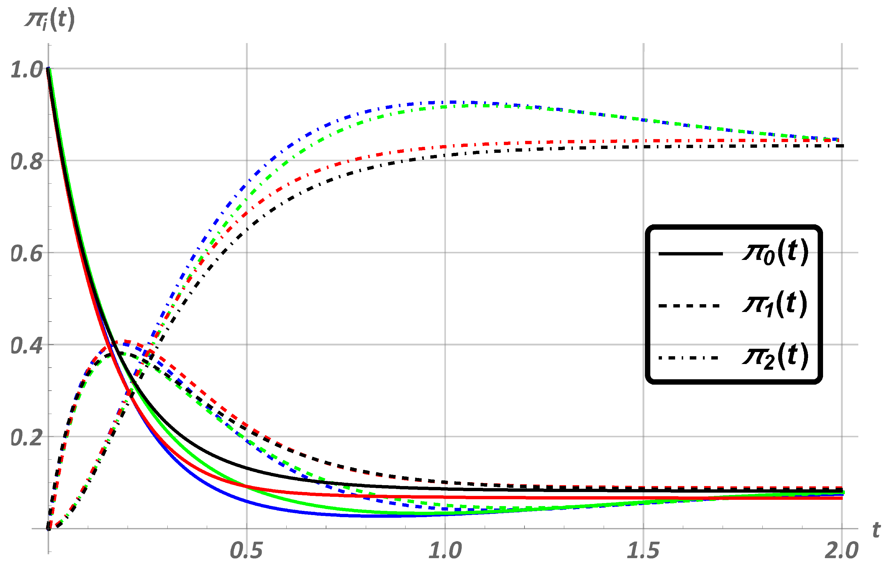
For components’ and system’s repair times, consider various combinations of Erlang distribution with different coefficients of variation. In each example, mean times and coefficients of variation are fixed, and through them, according to the formulas above, the corresponding distribution parameters are calculated. Figure 3 demonstrates the first example and the next step in the SA procedure.

The description of Figure 3 is the following:

• The legend of the figure denotes the types of lines of different probabilities; a simple line corresponds to probability ${\pi }_0\left(t\right)$, a dashed line corresponds to probability ${\pi }_1\left(t\right)$, and a dot–dash line corresponds to probability ${\pi }_2\left(t\right)$;
• Black color corresponds to $b=f=1$, $v_b=v_f=1$ (coinciding with Formulas (7) from Remark 1);
• Blue color corresponds to $b=f=1$, $v_b=v_f=0.5$;
• Red color corresponds to $b=f=1$, $v_b=0.5$, $v_f=1$;
• Green color corresponds to $b=f=1$, $v_b=1$, $v_f=0.5$.

Figure 3 shows similar behavior of the curves; they are very close to each other despite the different values of $v_b$ and $v_f$. At the same time, at the interval $t=[0.3,1.2]$, one can note a special contribution of the coefficient of variation of the system repair time $v_f$. For example, the blue and green probability curves for ${\pi }_2\left(t\right)$ lie above the black and red ones and are non-monotonic. Nevertheless, as t increases, the differences between the curves disappear and the characteristics pass into a stationary regime.

As the second example, consider the case when system’s repair time is twice that of the component repair one, $f=2$. This situation is presented in Figure 4. All notations are the same from the previous case,

• The legend of the figure denotes the type of line of different probabilities; a simple line corresponds to probability ${\pi }_0\left(t\right)$, a dashed line corresponds to probability ${\pi }_1\left(t\right)$, and a dot–dash line corresponds to probability ${\pi }_2\left(t\right)$;
• Black color corresponds to $b=1$, $f=2$, $v_b=v_f=1$;
• Blue color corresponds to $b=f=1$, $v_b=v_f=0.5$;
• Red color corresponds to $b=1$, $f=2$, $v_b=0.5$, $v_f=1$;
• Green color corresponds to $b=1$, $f=2$, $v_b=1$, $v_f=0.5$.

In this example, we observe the same behavior of the curves as in the first experiment regarding the influence of $v_f$ on t.d.s.s.p. If the coefficient of variation $v_f$ is less than $v_b$, the behavior of the curves on a small interval t changes, and the characteristics are non-monotonic.

Both examples show that the different values of $v_b$ and $v_f$ do not affect t.d.s.s.p.’s behavior with increasing t. It can be concluded that the system’s time-dependent characteristics are insensitive to the coefficient of variation of both repair times. Moreover, as $t\to \infty$, t.d.s.s.p. tend to their stationary values and turn to s.s.p.’s.

This section demonstrates the procedure of SA performed on an example of a 2-out-of-6 system for t.d.s.s.p.’s. In the next section, an SA of s.s.p.’s of a k-out-of-n system is presented.

5. Steady-State Probabilities

A stationary system’s characteristics can be calculated as a limit transition from LT of time-dependent probabilities,

$${\pi }_i=\underset{s\to 0}{lim}s{\tilde{\pi }}_i\left(s\right).$$

However, another way is also possible. Consider again arbitrary k and n.

5.1. System of Balance Equations and Its Solution

Since the process $Z\left(t\right)$ is a Harris one with a positive atom in the state 0, it has a stationary regime, and therefore, as $t⟶\infty$, its t.d.s.s.p.’s tend to corresponding s.s.p.’s,

$${\pi }_0=\underset{t\to \infty }{lim}{\pi }_0\left(t\right),{\pi }_i\left(x\right)=\underset{t\to \infty }{lim}{\pi }_i(t,x),i=\overline{1,k}.$$

The graphical results of the previous example also confirm this fact.

It means that the process $Z\left(t\right)$ has a stationary probability distribution for which the stationary regime differential equations (balance equations) hold with a corresponding transition in the systems (4)–(6). Thus, one can write down the following system,

$$\begin{array}{cc}\hfill {\lambda }_0{\pi }_0& ={\int }_0^{\infty }\beta \left(x\right){\pi }_1\left(x\right)dx+\underset{0}{\overset{\infty }{\int }}\varphi \left(x\right){\pi }_k\left(x\right)dx,\hfill \\ \hfill {\displaystyle \frac{d}{dx}}{\pi }_1\left(x\right)& =-({\lambda }_1+\beta \left(x\right)){\pi }_1\left(x\right),\hfill \\ \hfill {\displaystyle \frac{d}{dx}}{\pi }_i\left(x\right)& =-({\lambda }_i+\beta \left(x\right)){\pi }_i\left(x\right)+{\lambda }_{i-1}{\pi }_{i-1}\left(x\right),i=\overline{2,k-1},\hfill \\ \hfill {\displaystyle \frac{d}{dx}}{\pi }_k\left(x\right)& =-\varphi \left(x\right){\pi }_k\left(x\right),\hfill \end{array}$$

(8)

jointly with boundary conditions

$$\begin{array}{cc}\hfill {\pi }_1\left(0\right)& ={\lambda }_0{\pi }_0+{\int }_0^{\infty }\beta \left(x\right){\pi }_2\left(x\right)dx,\hfill \\ \hfill {\pi }_i\left(0\right)& ={\int }_0^{\infty }\beta \left(x\right){\pi }_{i+1}\left(x\right)dx,i=\overline{2,k-2},\hfill \\ \hfill {\pi }_{k-1}\left(0\right)& =0,\hfill \\ \hfill {\pi }_k\left(0\right)& ={\lambda }_{k-1}{\int }_0^{\infty }{\pi }_{k-1}\left(x\right)dx.\hfill \end{array}$$

(9)

The application of the method of constant variation to expressions (8) and (9) gives the following result.

Theorem 2.

The s.s.p.’s of the process $Z\left(t\right)$ in terms of LT of components’ repair time in point ${\lambda }_i$, $\tilde{b}\left({\lambda }_i\right),i=1,2$, and mean system’s repair time f have the form

$$\begin{array}{cc}\hfill {\pi }_0& ={\lambda }_0^{-1}\left[C_1\left(1+\frac{{\lambda }_1}{{\lambda }_1-{\lambda }_2}\tilde{b}\left({\lambda }_1\right)\right)-C_2\tilde{b}\left({\lambda }_2\right)\right],\hfill \\ \hfill {\pi }_1& =C_1{\displaystyle \frac{1-\tilde{b}\left({\lambda }_1\right)}{{\lambda }_1}},\hfill \\ \hfill {\pi }_i& =C_i{\displaystyle \frac{1-\tilde{b}\left({\lambda }_i\right)}{{\lambda }_i}}+\mathrm{S}(i-1){\displaystyle \frac{1-\tilde{b}\left({\lambda }_{i-1}\right)}{{\lambda }_{i-1}}},i=\overline{2,k-1},\hfill \\ \hfill {\pi }_k& =C_k·f,\hfill \end{array}$$

(10)

where

$$\begin{array}{cc}\hfill & C_i=C_{i+1}\tilde{b}\left({\lambda }_{i+1}\right)+\mathrm{S}\left(i\right)\tilde{b}\left({\lambda }_i\right)-\mathrm{S}(i-1),i=\overline{2,k-2},\hfill \\ \hfill & C_{k-1}=-\mathrm{S}(k-2),\hfill \\ \hfill & C_k={\lambda }_{k-1}{C}_{k-1}\left({\displaystyle \frac{1-\tilde{b}\left({\lambda }_{k-1}\right)}{{\lambda }_{k-1}}}-{\displaystyle \frac{1-\tilde{b}\left({\lambda }_{k-2}\right)}{{\lambda }_{k-2}}}\right),\hfill \\ \hfill & \mathrm{S}\left(i\right)=\sum _{j=1}^i{(-1)}^{i-j+1}\left(\prod _{m=j}^i{\displaystyle \frac{{\lambda }_m}{{\lambda }_j-{\lambda }_{m+1}}}\right)C_j,\hfill \end{array}$$

(11)

and $C_1$ is calculated according to the normalization condition ${\sum }_{i\in E}{\pi }_i=1$.

Proof. 

The general idea of the proof consists in the application of the method of constant of variation. In this way, probabilities ${\pi }_i\left(x\right),i=\overline{1,k}$ have the following form,

$$\begin{array}{cc}\hfill {\pi }_1\left(x\right)& =C_1{e}^{-{\lambda }_{1}x}(1-B\left(x\right)),\hfill \\ \hfill {\pi }_i\left(x\right)& =C_i\left(x\right)e^{-{\lambda }_{i}x}(1-B\left(x\right)),i=\overline{2,k-1},\hfill \\ \hfill {\pi }_k\left(x\right)& =C_k(1-F\left(x\right)),\hfill \end{array}$$

(12)

where function $C_i\left(x\right)$ follows from the substitution of the obtained expression for ${\pi }_1\left(x\right)$ into the solution of the heterogeneous equation of the system for ${\pi }_i\left(x\right)$,

$$\begin{array}{ccc}\hfill C_i\left(x\right)& =& C_i+\sum _{j=1}^{i-1}{(-1)}^{i-j+1}\left(\prod _{m=j}^i{\displaystyle \frac{{\lambda }_m}{{\lambda }_j-{\lambda }_{m+1}}}\right)C_j{e}^{-({\lambda }_{i-1}-{\lambda }_i)x}.\hfill \end{array}$$

Using boundary conditions (9) and expressions (12), one can obtain all the constants $C_i,i=\overline{2,k}$. The completion of the theorem is the calculation of the probability ${\pi }_0$ from the first equation of (8), followed by the application of the normalization condition ${\sum }_{i\in E}{\pi }_i=1$ to calculate the final constant $C_1$. □

Expressions (10) and (11) show that s.s.p.’s depend on the shape of components’ repair time distribution, while the system’s repair time is presented as the mean value, which is distribution-independent.

For numerical and sensitivity analysis, consider the application of Theorem 2 on the example of a 3-out-of-6 model. Such an example corresponds to a mathematical model of an automated system for remote monitoring of an underwater pipeline [29] and is useful in the reliability study of such a technical system.

The s.s.p.’s for the 3-out-of-6 system with inverse substitution ${\lambda }_i=(n-i)\alpha ,i=\overline{0,k-1}$ have the following form,

$$\begin{array}{cc}\hfill & {\pi }_1={\displaystyle \frac{6}{5}}·\frac{1-\tilde{b}\left(5\alpha \right)}{1+5\tilde{b}\left(5\alpha \right)-5\tilde{b}\left(4\alpha \right)}{\pi }_0,{\pi }_2={\displaystyle \frac{3}{2}}·{\displaystyle \frac{1+4\tilde{b}\left(5\alpha \right)-5\tilde{b}\left(4\alpha \right)}{1+5\tilde{b}\left(5\alpha \right)-5\tilde{b}\left(4\alpha \right)}}{\pi }_0,\hfill \\ \hfill & {\pi }_3={\displaystyle \frac{6\alpha f(1+4\tilde{b}\left(5\alpha \right)-5\tilde{b}\left(4\alpha \right))}{1+5\tilde{b}\left(5\alpha \right)-5\tilde{b}\left(4\alpha \right)}}{\pi }_0,\hfill \\ \hfill & {\pi }_0={\displaystyle \frac{10(1+5\tilde{b}\left(5\alpha \right)-5\tilde{b}\left(4\alpha \right))}{37+60\alpha f-25\tilde{b}\left(4\alpha \right)(5+12\alpha f)+2\tilde{b}\left(5\alpha \right)(49+120\alpha f)}},\hfill \end{array}$$

(13)

and the availability coefficient is

$$\begin{array}{c}\hfill K_{av}=1-{\pi }_3={\displaystyle \frac{37+98\tilde{b}\left(5\alpha \right)-125\tilde{b}\left(4\alpha \right)}{37+60\alpha f-25\tilde{b}\left(4\alpha \right)(5+12\alpha f)+2\tilde{b}\left(5\alpha \right)(49+120\alpha f)}}.\end{array}$$

(14)

Remark 2.

Note that, analogous to Remark 1, if $B\left(x\right)=1-e^{-x{b}^{-1}}$, the result corresponds to the probabilities obtained by a simple birth and death process,

$$\begin{array}{cc}\hfill & {\pi }_0={\displaystyle \frac{20{\alpha }^2{b}^2+4\alpha b+1}{120{\alpha }^3{b}^{2}f+74{\alpha }^2{b}^2+10\alpha b+1}},{\pi }_1={\displaystyle \frac{24{\alpha }^2{b}^2+6\alpha b}{120{\alpha }^3{b}^{2}f+74{\alpha }^2{b}^2+10\alpha b+1}},\hfill \\ \hfill & {\pi }_2={\displaystyle \frac{30{\alpha }^2{b}^2}{120{\alpha }^3{b}^{2}f+74{\alpha }^2{b}^2+10\alpha b+1}},{\pi }_3={\displaystyle \frac{120{\alpha }^3{b}^{2}f}{120{\alpha }^3{b}^{2}f+74{\alpha }^2{b}^2+10\alpha b+1}},\hfill \\ \hfill & K_{av}={\displaystyle \frac{74{\alpha }^2{b}^2+10\alpha b+1}{120{\alpha }^3{b}^{2}f+74{\alpha }^2{b}^2+10\alpha b+1}}.\hfill \end{array}$$

(15)

5.2. Sensitivity Analysis: Rare Failures

The s.s.p.’s from Theorem 2, as well as the Formulas (13) and (14) derived from it, are presented in terms of the LT of repair time distribution of the system components. Thence, the evident dependence of these probabilities on the shape of the repair-time distribution is observed. On the other hand, some earlier papers show that with “rare” failures, the shape of such a distribution does not affect the reliability measures. This property is called insensitivity. In this section, we consider the behavior of the s.s.p.’s and their insensitivity under the rare failures condition.

For the considered model, the rare failures should be understood as the low failures’ intensity with respect to the fixed mean repair time. Thus, suppose that $\alpha \to 0$, which consequently leads to the following result.

Applying the Taylor series up to the second order of $\alpha$,

$$\tilde{b}\left({\lambda }_i\right)\approx 1-b{\lambda }_i+{\displaystyle \frac{b^2{\lambda }_i^2}{2}},i=1,2,$$

with substitution ${\rho }_1=\alpha b$ and ${\rho }_2=\alpha f$ from (13) and (14), the following expressions hold,

$$\begin{array}{cc}\hfill {\pi }_1& \approx {\displaystyle \frac{6{\rho }_1(2-5{\rho }_1)}{2-5{\rho }_1(2-9{\rho }_1)}}{\pi }_0,{\pi }_2\approx {\displaystyle \frac{30{\rho }^2}{2-5{\rho }_1(2-9{\rho }_1)}}{\pi }_0,\hfill \\ \hfill {\pi }_3& \approx {\displaystyle \frac{120{\rho }_1^2{\rho }_2}{2-5{\rho }_1(2-9{\rho }_1)}}{\pi }_0,{\pi }_0\approx {\displaystyle \frac{2-5{\rho }_1(2-9{\rho }_1)}{2+{\rho }_1(2+15{\rho }_1(3+8{\rho }_2))}},\hfill \\ \hfill K_{av}& \approx {\displaystyle \frac{2+2{\rho }_1+45{\rho }_1^2}{2+{\rho }_1(2+15{\rho }_1(3+8{\rho }_2))}}.\hfill \end{array}$$

(16)

Consider some further numerical examples for the SA performance of s.s.p.’s of the 3-out-of-6 model in terms of the shape of the repair time distribution as well as its coefficient of variation $v_b=v$.

The following distributions are used for the repair time:

• Erlang ($Erl=Erl(l,\theta )$) with notations as above;
• Gnedenko–Weibull ($GW=GW(k,\lambda )$), for which

  $$b\left(t\right)={\displaystyle \frac{k}{\lambda }}{\left({\displaystyle \frac{t}{\lambda }}\right)}^{k-1}{e}^{-{(t/\lambda )}^k},t>0,\tilde{b}\left(s\right)={\displaystyle \frac{k}{{\lambda }^k}}{\int }_0^{\infty }{e}^{-st-{(t/\lambda )}^k}{t}^{k-1}dt,$$

  $$b=\lambda ·\Gamma \left(1+\frac{1}{k}\right),v=\frac{\sqrt{{\lambda }^2·\Gamma (1+2/k)-b^2}}{b};$$
• Uniform ($U=U(\widehat{a},\widehat{b})$), for which

  $$b\left(t\right)={\displaystyle \frac{1}{\widehat{b}-\widehat{a}}},t\in [\widehat{a},\widehat{b}],\tilde{b}\left(s\right)={\displaystyle \frac{e^{-\widehat{a}s}-e^{-\widehat{b}s}}{s(\widehat{b}-\widehat{a})}},b={\displaystyle \frac{\widehat{a}+\widehat{b}}{2}},v={\displaystyle \frac{1}{\widehat{a}+\widehat{b}}}·\sqrt{{\displaystyle \frac{{(\widehat{b}-\widehat{a})}^2}{3}}}.$$

Note that if $v=1$, $Erl$ and $GW$ distributions pass to the exponential one with the mean time b. Then, the s.s.p.’s coincide with the Formula (15) from Remark 2.

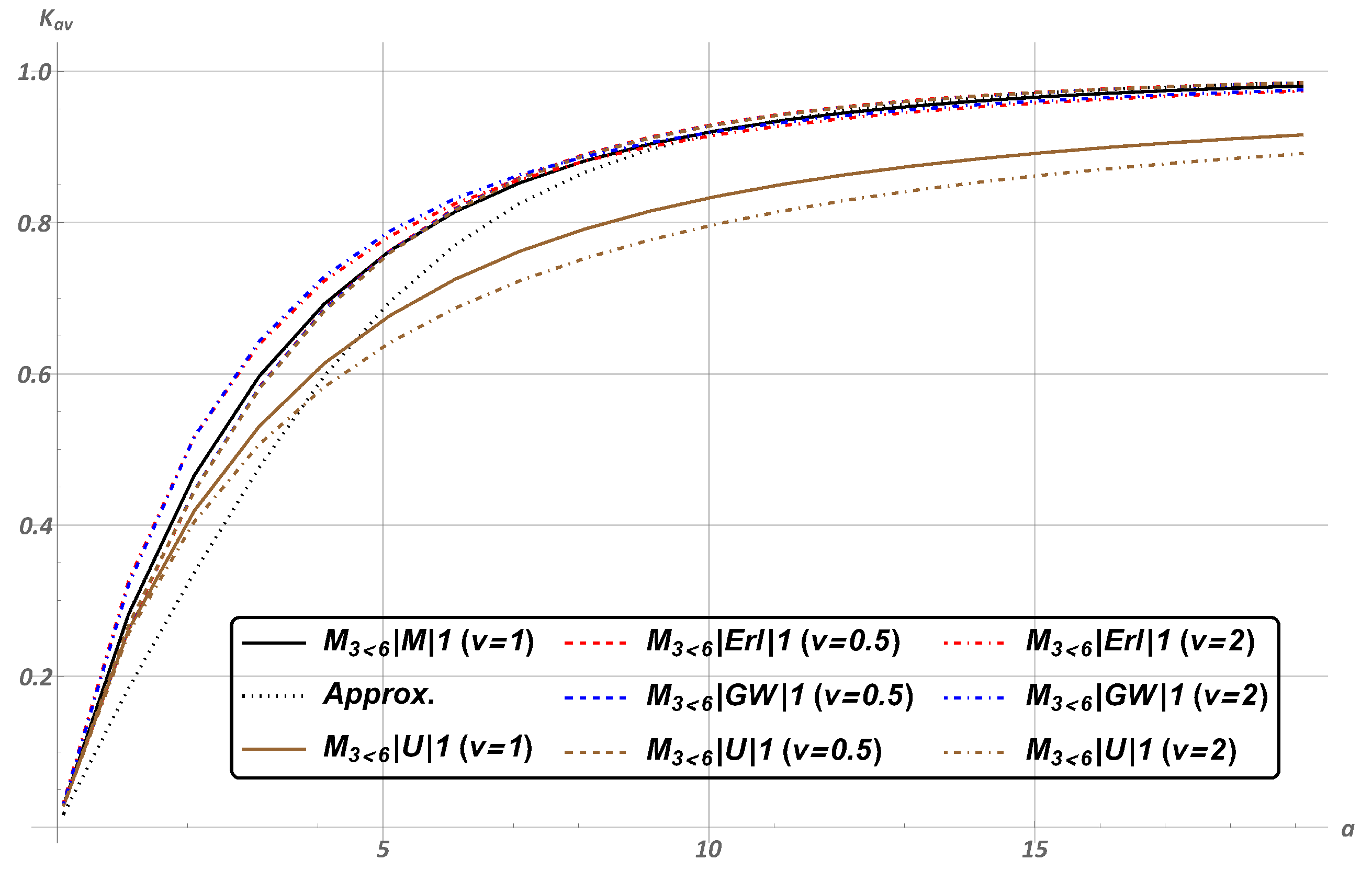
Suppose $b=1$, $v=0.5,1,2$, and mean system’s repair time $f=2$. Since s.s.p.’s do not depend on the shape of the system’s repair time distribution $F\left(x\right)$ but only on the mean f, the corresponding coefficient of variation is not fixed. The mean lifetime of system elements $a=\overline{0.1,20}$, and then the failure intensity $\alpha =a^{-1}$ decreases. Figure 5 shows the graphical representation of the dependence of the coefficient of availability $K_{av}$ from the mean lifetime of system elements for different repair time distributions, as well as the case of rare failures (in the legend, it is defined as Approx.).

This figure shows that over the entire interval a under consideration, all curves become very close to each other despite the different values of v. As $a\approx 10$, the curve corresponding to the asymptotic expression (16), which is defined as Approx., merges with other ones that correspond to $\langle M_{3<6}\left|Erl\right|1\rangle$ and $\langle M_{3<6}\left|GW\right|1\rangle$ models and $\langle M_{3<6}\left|U\right|1\rangle$ models with $v=0.5$.

On the other hand, as $v=1,2$ in the $\langle M_{3<6}\left|U\right|1\rangle$ model, the corresponding curves of $K_{av}$ reach other ones slower.

Table 1. $K_{av}$ of $\langle M_{3<6}\left|GI\right|1\rangle$ system under rare failures.

		$\mathit{a}=20$	$\mathit{a}=40$	$\mathit{a}=80$	$\mathit{a}=200$
$\langle M_{3<6}\left|M\right|1\rangle$	$v=1$	$0.9825$	$0.9971$	$0.9996$	$0.9999$
Approx. (16)		$0.9866$	$0.9982$	$0.9998$	$0.9999$
$\langle M_{3<6}\left|U\right|1\rangle$	$v=0.5$	$0.9864$	$0.9980$	$0.9997$	$0.9999$
	$v=1$	$0.9198$	$0.9606$	$0.9802$	$0.9920$
	$v=2$	$0.8958$	$0.9476$	$0.9735$	$0.9893$
$\langle M_{3<6}\left|Erl\right|1\rangle$	$v=0.5$	$0.9865$	$0.9980$	$0.9997$	$0.9999$
	$v=2$	$0.9761$	$0.9950$	$0.9992$	$0.9999$
$\langle M_{3<6}\left|GW\right|1\rangle$	$v=0.5$	$0.9774$	$0.9951$	$0.9991$	$0.9999$
	$v=2$	$0.9863$	$0.9979$	$0.9997$	$0.9999$

presents the availability coefficient with increasing a. According to the table, even as $a=200$, the coefficient of availability $K_{av}$ of the $\langle M_{3<6}\left|U\right|1\rangle$ model with $v\ge 1$ does not show the absolute accuracy with other ones and with the case of rare failures.

Nevertheless, the results indicate the insensitivity of the stationary characteristics of the k-out-of-n system to the shape of the repair time distribution and the value of its coefficient of variation.

5.3. Sensitivity Analysis: Quick Restoration

On the other hand, the sensitivity of the system’s stationary characteristics in the case of quick restoration is also of interest. Suppose now that the mean lifetime a is fixed for all repair time distributions, $a=1$. As distributions of the repair time, the above ones are also used.

Suppose $f=2·b$, the coefficients of variation of components’ repair are the following, $v=0.1,0.5,1,5,10$. As a model parameter, consider the value,

$$\rho ={\displaystyle \frac{a}{b}}={\displaystyle \frac{\mathrm{restoration}\mathrm{rate}}{\mathrm{failure}\mathrm{rate}}},$$

which can be interpreted as a relative rate of the system’s components recovery. The results of this example are shown in Figure 6.

The description of Figure 6 is the following:

• The legend of the figure denotes the type of line of different coefficient of variation v; a simple line corresponds to $v=0.1$, a dashed line means $v=0.5$, a dot–dash line is for $v=1$, a dotted line is for $v=5$ and a dashed with two dots means $v=10$;
• Blue color corresponds to $\langle M_{3<6}\left|Erl\right|1\rangle$;
• Red color corresponds to $\langle M_{3<6}\left|GW\right|1\rangle$;
• Brown color corresponds to $\langle M_{3<6}\left|U\right|1\rangle$.

According to Figure 6, the considered distributions of repair time show a similar behavior of availability curves as $v\le 1$. That is, in the case of quick restoration, as $\rho$ increases, $v\le 1$ system’s stationary characteristics are asymptotically insensitive to the shape of the repair-time distribution as well as its coefficient of variation with fixed mean repair time and corresponding v. As $v>1$, the curves’ behavior is different. At small $\rho$, as $v=5,10$ in $\langle M_{3<6}\left|Erl\right|1\rangle$ and $\langle M_{3<6}\left|GW\right|1\rangle$, model curves of $K_{av}$ rather quickly tend to 1 and as $\rho \approx 10$, they take values close to other curves.

Furthermore, the coefficient of availability $K_{av}$ of the $\langle M_{3<6}\left|U\right|1\rangle$ model shows slower convergence to 1 as $v>1$. In can be concluded that for small $\rho$ (and large b), the system’s characteristics are sensitive both to the shape of the repair-time distribution and to the value of the coefficient of variation v at a fixed mean b.

Table 2. $K_{av}$ of $\langle M_{3<6}\left|GI\right|1\rangle$ system under quick restoration.

		$\mathit{\rho }=20$	$\mathit{\rho }=40$	$\mathit{\rho }=80$	$\mathit{\rho }=200$
$\langle M_{3<6}\left|M\right|1\rangle$	$v=1$	$0.9825$	$0.9971$	$0.9996$	$0.9999$
$\langle M_{3<6}\left|Erl\right|1\rangle$	$v=0.1$	$0.9883$	$0.9983$	$0.9998$	$0.9999$
	$v=0.5$	$0.9865$	$0.9980$	$0.9997$	$0.9999$
	$v=5$	$0.9784$	$0.9933$	$0.9983$	$0.9998$
	$v=10$	$0.9879$	$0.9955$	$0.9985$	$0.9997$
$\langle M_{3<6}\left|GW\right|1\rangle$	$v=5$	$0.9796$	$0.9944$	$0.9987$	$0.9998$
	$v=10$	$0.9863$	$0.9958$	$0.9988$	$0.9998$
$\langle M_{3<6}\left|U\right|1\rangle$	$v=5$	$0.8618$	$0.9681$	$0.9949$	$0.9996$
	$v=10$	$0.8053$	$0.9208$	$0.9826$	$0.9986$

presents $K_{av}$ for large $\rho$ for some cases of repair-time distributions and their coefficients of variation. Since all curves of $K_{av}$ show very close results to $v\le 1$, the table contains calculations only for one case of the repair-time distribution ($Erl$) as $v\le 1$.

Table 2 proves, as $\rho \to \infty$ and $v>1$, the system’s availability tends to 1 slower. However, as $\rho =200$$K_{av}\approx 0.9999$ for all repair time distributions and $v>1$. The results provided in Table 2 and Figure 6 indicate the presence of asymptotic insensitivity of the system’s stationary characteristics to the shape of the repair time distribution and its coefficient of variation at a fixed mean and $\rho \to \infty$.

6. Discussion and Conclusions

In this article, the general procedure for sensitivity analysis performance is introduced and proposed for a reliability study of technical systems and mathematical models corresponding to them. The presented procedure is universal, since it can be successfully applied to many mathematical models to carefully study the influence of their initial parameters on the target characteristics.

The proposed study, and SA itself, covers a wide range of practical tasks in technical issues. For example, it is useful in the following situations.

• Usually, information about life and repair time distributions of components of a real technical system is unknown. If corresponding statistical data are available, the first moments of these times (mean and variance) can be estimated. However, in the absence of such information, one can only make assumptions about this. In such situations, SA is necessary for understanding the system operation and the impact of its input data on the system behavior.
• The impact of the initial parameters on system performance is not always obvious. The conclusions followed from SA can serve as recommendations to engineers and developers in the framework of improving the reliability of a technical system.

In the example of the repairable k-out-of-n system, the SA procedure is discussed, and the probabilistic characteristics of its reliability of this model are investigated. The paper considers the k-out-of-n system with exponential lifetime and arbitrary repair time distribution, and the sensitivity of its reliability measures to repair-time distribution and its coefficient of variation. According to SA methodology, the following steps were conducted, and new results were obtained.

Step 1. The method of supplementary variables, which helps to study t.d.s.s.p.’s and s.s.p.’s, was used and applied to study the k-out-of-n system.

Step 2. The sensitivity of t.d.s.s.p.’s with the Erlang distribution of repair time to its coefficient of variation was studied on the example of the 2-out-of-6 model. Numerical analysis showed insensitivity of these characteristics to the value of the coefficient of variation of both components’ and system’s repair time as $t\to \infty$. On the other hand, as $t\to \infty$, t.d.s.s.p.’s tend to their stationary values and turn to s.s.p.’s.

Step 3. An explicit form of s.s.p.’s of the k-out-of-n model in terms of LT of the repair-time distribution was presented. Numerical experiments showed asymptotic insensitivity of s.s.p.’s of the 3-out-of-6 system to the shape of the repair-time distribution, its coefficient of variation under rare failures, and quick restoration conditions of the system’s components.

Further research will continue studies of a k-out-of-n system in the direction of reliability and sensitivity analysis, including the dependencies of a system’s failure on the location of failed components; a load-sharing k-out-of-n system in which a component’s failure influences the increase in load of the other components remaining operational and therefore decreases their residual lifetime.

References

- Kala, Z.; Omishore, A. Reliability and Sensitivity Analyses of Structures Related to Eurocodes. Int. J. Mech. 2022, 16, 98–107. [Google Scholar] [CrossRef]
- Saltelli, A.; Chan, K.; Scott, E.M. Sensitivity Analysis; John Wiley & Sons: New York, NY, USA, 2000. [Google Scholar]
- Borgonovo, E.; Plischke, E. Sensitivity analysis: A review of recent advances. Eur. J. Oper. Res. 2016, 248, 869–887. [Google Scholar] [CrossRef]
- Sevast’yanov, B.A. An Ergodic Theorem for Markov Processes and Its Application to Telephone Systems with Refusals. Theory Probab. Its Appl. 1957, 2, 104–112. [Google Scholar] [CrossRef]
- Gertsbakh, I.B. Asymptotic methods in reliability theory: A review. Adv. Appl. Probab. 1984, 16, 147–175. [Google Scholar] [CrossRef]
- Zachary, S. A Note on Insensitivity in Stochastic Networks. J. Appl. Probab. 2007, 44, 238–248. [Google Scholar] [CrossRef] [Green Version]
- Kovalenko, I.N. Investigations on Analysis of Complex Systems Reliability; Naukova Dumka: Kiev, Ukraine, 1976. (In Russian) [Google Scholar]
- Rykov, V. Multidimensional alternative processes reliability models. In Proceedings of the BWWQT Conference, Minsk, Belarus, 28–31 January 2013; Dudin, A., Klimenok, V., Tsarenkov, G., Dudin, S., Eds.; Springer: Berlin, Germany, 2013; pp. 147–156. [Google Scholar] [CrossRef]
- Ivnitzkii, V.A. On a Condition of the Invariance of Stationary Probabilities of States for Networks of Sequential Queuing Systems. Theory Probab. Appl. 1989, 34, 519–523. [Google Scholar] [CrossRef]
- Ivnitzkii, V.A. On the Invariance of Stationary State Probabilities of a Non-Product-Form Single-Line Queueing System. Probl. Inform. Transm. 2002, 38, 368–376. [Google Scholar] [CrossRef]
- Eremina, A. Invariance of the stationary state distribution for mass service networks with multi-regime strategies, different demands, and a “generalized processor sharing” discipline. Autom. Control. Comput. Sci. 2011, 45, 29–38. [Google Scholar] [CrossRef]
- Dovzhenok, T. Invariance of the Stationary Distribution of Networks with Bypasses and “Negative” Customers. Autom. Remote Control. 2002, 63, 1458–1469. [Google Scholar] [CrossRef]
- Boyarovich, Y.S. The stationary distribution invariance of states in a closed queueing network with temporarily non-active customers. Autom. Remote Control. 2012, 73, 1616–1623. [Google Scholar] [CrossRef]
- Schassberger, R. Insensitivity of Steady-State Distributions of Generalized Semi-Markov Processes. Part I. Ann. Probab. 1977, 5, 87–99. [Google Scholar] [CrossRef]
- Schassberger, R. Insensitivity of Steady-State Distributions of Generalized Semi-Markov Processes. Part II. Ann. Probab. 1978, 6, 88–95. [Google Scholar] [CrossRef]
- Morozov, E.; Pagano, M.; Peshkova, I.; Rumyantsev, A. Sensitivity Analysis and Simulation of a Multiserver Queueing System with Mixed Service Time Distribution. Mathematics 2020, 8, 1277. [Google Scholar] [CrossRef]
- Efrosinin, D.; Rykov, V. Sensitivity Analysis of Reliability Characteristics to the Shape of the Life and Repair Time Distributions. In Proceedings of the 13th International Scientific Conference, Information Technologies and Mathematical Modeling, Anzhero-Sudzhensk, Russia, 20–22 November 2014; Dudin, A., Nazarov, A., Yakupov, R., Gortsev, A., Eds.; Springer: Berlin, Germany, 2014; 487. [Google Scholar] [CrossRef]
- Rykov, V.; Zaripova, E.; Ivanova, N.; Shorgin, S. On Sensitivity Analysis of Steady State Probabilities of Double Redundant Renewable System with Marshal-Olkin Failure Model. In Proceedings of the Distributed Computer and Communication Networks Conference, Moscow, Russia, 17–21 September 2018; Vishnevskiy, V.V., Kozyrev, D.V., Eds.; Springer: Berlin, Germany, 2018; pp. 234–245. [Google Scholar]
- Efrosinin, D.; Stepanova, N.; Sztrik, J.; Plank, A. Approximations in Performance Analysis of a Controllable Queueing System with Heterogeneous Servers. Mathematics 2020, 8, 1803. [Google Scholar] [CrossRef]
- Genis, Y. On Reliability of Systems with Periodic Maintenance under Rare Failures of Its Elements. Autom. Remote Control. 2010, 71, 1337–1345. [Google Scholar] [CrossRef]
- Ivanova, N. On Steady State Reliability and Sensitivity Analysis of a k-out-of-n System under Full Repair Scenario. In Proceedings of the Distributed Computer and Communication Networks Conference, Moscow, Russia, 26–29 September 2022; Vishnevskiy, V.M., Samouylov, K.E., Kozyrev, D.V., Eds.; Springer: Berlin, Germany, 2022; Volume 13766. [Google Scholar] [CrossRef]
- Houankpo, H.G.K.; Kozyrev, D. Mathematical and Simulation Model for Reliability Analysis of a Heterogeneous Redundant Data Transmission System. Mathematics 2021, 9, 2884. [Google Scholar] [CrossRef]
- Zuo, M.J.; Tian, Z. k-out-of-n Systems. In Wiley Encyclopedia of Operations Research and Management Science; Cochran, J.J., Ed.; Wiley: New York, NY, USA, 2010. [Google Scholar]
- Nguyen, D.P.; Kozyrev, D.V. Reliability Analysis of a Multirotor Flight Module of a High-altitude Telecommunications Platform Operating in a Random Environment. In Proceedings of the International Conference of Engineering and Telecommunication (En & T), Dolgoprudny, Russia, 25–26 November 2020; pp. 1–5. [Google Scholar] [CrossRef]
- Cox, D.R. The analysis of non-Markovian stochastic processes by the inclusion of supplementary variables. Math. Proc. Camb. Phil. Soc. 1955, 51, 433–441. [Google Scholar] [CrossRef]
- Dimitrov, B.; Rykov, V. On k-out-of-n System Under Full Repair and Arbitrary Distributed Repair Time. In Proceedings of the Distributed Computer and Communication Networks: Control, Computation, Communications Conference, Moscow, Russia, 26–29 September 2021; Vishnevskiy, V.M., Samouylov, K.E., Kozyrev, D.V., Eds.; Springer: Berlin, Germany, 2021; 13144. [Google Scholar] [CrossRef]
- Rykov, V.; Ivanova, N.; Kozyrev, D. Sensitivity Analysis of a k-out-of-n:F System Characteristics to Shapes of Input Distribution. Lect. Notes Comput. Sci. (LNCS) 2020, 12563, 485–496. [Google Scholar] [CrossRef]
- Rykov, V.; Ivanova, N.; Kozyrev, D. Application of Decomposable Semi-Regenerative Processes to the Study of k-out-of-n Systems. Mathematics 2021, 9, 1933. [Google Scholar] [CrossRef]
- Rykov, V.; Kochueva, O.; Farkhadov, M. Preventive Maintenance of a k-out-of-n System with Applications in Subsea Pipeline Monitoring. J. Mar. Sci. Eng. 2021, 9, 85. [Google Scholar] [CrossRef]
Figure 1.
The general procedure for SA performance.
Figure 2.
Transition graph of the process , which described the behavior of a k-out-of-n model.
Figure 3.
T.d.s.s.p.’s of system () with different values of coefficients of variation of components and system repair time.
Figure 4.
T.d.s.s.p.’s of (, ) with different values of coefficients of variation of components and system repair time.
Figure 5.
of a 3-out-of-6 system under the rare failures’ scenario with different repair time distributions and coefficients of variation v.
Figure 6.
of a 3-out-of-6 system under quick components’ repair scenario with different repair time distributions and coefficients of variation v.