Modified Finite Element Study for Heat and Mass Transfer of Electrical MHD Non-Newtonian Boundary Layer Nanofluid Flow

Abstract

Research into the effects of different parameters on flow phenomena is necessary due to the wide range of potential applications of non-Newtonian boundary layer nanofluid flow, including but not limited to production industries, polymer processing, compression, power generation, lubrication systems, food manufacturing, and air conditioning. Because of this impetus, we investigated non-Newtonian fluid flow regimes from the perspectives of both heat and mass transfer aspects. In this study, heat transfer of electrical MHD non-Newtonian flow of Casson nanofluid over the flat plate is investigated under the effects of variable thermal conductivity and mass diffusivity. Emerging problems occur as nonlinear partial differential equations (NPDEs) in opposition to the conservation laws of mass, momentum, heat, and species transportation. The shown problem can be recast as a set of ordinary differential equations by making the necessary changes. A modified finite element method is adopted to solve the obtained set of ODEs. The numerical method is based on Galerkin weighted residual approach, and Gauss–Legendre numerical integration is adopted in the modified finite element method application procedure. To clarify the obtained results, another numerical technique is employed to solve the reduced ODEs. With the help of error tables and the flowing behavior of complicated physical parameters on estimated solutions, this study graphically and tabulatively explains the convergence of analytic solutions. Comparing some of the obtained results with those given in past research is also done. From the obtained results, it is observed that the velocity profile escalates by improving the electric parameter. Our intention is for this paper to serve as a guide for academics in the future who will be tasked with addressing pressing issues in the field of industrial and engineering enclosures.

1. Introduction

Recently, heat transport has gained attraction in the engineering and manufacturing fields due to its extensive applications in several mechanical industries. It is challenging to control heat transport by increasing the surface area of heat exchange, which is highly difficult to maintain in heat-managing systems. For the past few years, engineers have been trying to make large surface areas for heat to exchange but have failed owing to the weak thermophysical properties of conventional fluids. Water, alcohol, ethylene glycol, and oil are conventional fluids. These fluids’ thermal conductivity can be managed by controlling heat transportation [1]. Nanofluids are the best example of high thermal conductive fluids whose suspension (like nanometer-sized metal oxides, metals, polymers, carbon nanotubes, or even silica particles) can quickly disperse in nanofluids [2]. In 1995, Choi [3] proposed using nanoparticles for the first time.

Increased thermal conductivity of fluid is beneficial because it reduces the clogging process in the walls of heat transport devices, increases energy competence, improves work, and is cost-effective [4] since nanofluids are thermally conductive and can be used as energy competence in heat transport devices. Souayeh et al. [5] observed the cooling properties of Casson nanofluid and suggested its use as a friction-controlling agent. His investigation involved the Prandtl boundary layer equation and some numerically supported facts with uniform variables. Alwaei et al. [6] applied the Keller-box method to study the electrically conducted Casson nanofluid flow on a hard-rounded object. The study involved the use of three nanoparticles, i.e., titanium dioxide (TiO₂), silver (Ag), and graphite oxide (GO), along with sodium alginate as a base fluid. Saqib et al. [7] constructed a Casson nanofluid based on Tiwari and Das model and molybdenum disulfide as a nanoparticle. Ethylene glycol was used as a base fluid to study integral transformation.

Entropy generation in nanofluids during heat transport was studied by Miles and Bessaih [8], who consider the flow of liquid in a circular annulus into operated in a perforated medium. Aglawe et al. [9]. Elaborated on using nanofluids to cool electronic systems and briefly explained the procedure of nanofluid formation along with some defies. The effect of thermal conductivity on the physical properties and rheology of nanofluid was determined by Tlili [10]. Archana et al. [11] worked on the Range-Kutta-Fehlberg scheme to find out the numerics of Casson fluid, its incompressibility and squeezing. Reddy et al. [12]. Studied the time dependant flow of Casson nanofluid with radiative heat transfer. This study proposed that the greater the value of the unsteady parameter greater will be the cooling rate. Lokesh et al. [13] inferred a fourth-order Runge–Kutta scheme when discussing the three-dimensional flow of Casson nanofluid. In support of the research, only a small number of numerical solutions were drawn.

Ref. [14] performed Casson fluid’s temperature and velocity analysis and the skin friction coefficient calculation. Magnetohydrodynamic conditions were set on perforated media, and findings revealed the rise in temperature due to increased heat generation. The Casson fluid flow’s chemical flow and heat absorbing attribute was examined by [15] with a wide and verticle plate. Using non-Darcy porous medium velocity, temperature and average skin fraction value were analyzed. Ref. [16] proved a direct relation of the magnetic parameter to shear wall stress, while an inverse relation was observed with respect to velocity. This was observed during a study conducted to calculate the behavior of MHD Casson fluid with a vertical plate with static temperature and shear wall stress. Ref. [17] revealed a reduced field velocity due to slip parameter using Laplace transformation. These were the observations of a study conducted on the non-Newtonian flow of Casson fluid over a plate under constant temperature. The skin friction coefficient is inversely proportional to the Hartman and Casson numbers, as studied in [18]. These results emerged from the study’s discussion of homotopy solutions for numerical analysis of heating and viscous effects at a constant temperature.

With the help of homotopy analysis, we can calculate the linear temperature functions responsible for thermal conduction and viscosity in an incompressible Casson fluid. As [19] demonstrated, a higher fluid viscosity causes a lower fluid temperature with increasing velocity. Casson fluid flow was examined by [20] to investigate the effects of fractional derivatives on the studied temperature and concentration parameters. The results demonstrated a positive correlation between temperature and velocity, leading to heat generation, with fluid velocity inversely correlated to the chemical reaction. The dynamics of submarine debris flow in the viscoplastic fluid using the Lagrangian equation was carried out by [21]. Various rheological models revealed that the downslope movement of dense fluid having constant volume could exhibit a transitional state between viscous and plastic. Similar observations were made by [22] using the Bingham model. The shear rate and viscosity of fluid calculated the yield surface. MHD Casson fluid flow was determined, and a study was conducted on non-Darcy porous media to study partial differential equations.

Velocity, concentration, and skin friction are the magnetic and Casson parameters that are directly related to temperature; however, the Casson parameter is directly related to skin friction. On the other hand, magnetic parameters are inversely proportional to skin friction [23]. Ref. [24] applied the Laplace Transformation technique to study the velocity and skin friction of visco-elastic incompressible fluid. The study was designed to provide a magnetic field over a finite accelerated plate in a porous medium. Findings revealed that velocity is directly linked to fluid permeability and elasticity, whereas skin friction increased with medium permeability. Ref. [25] investigated the Caputo fractional model of MHD Casson fluid flow using Fourier and Laplace transformation. Findings showed that the increased value of the Casson parameter would change the behavior of Casson fluid more closely to the Newtonian fluid. Qureshi et al. [26] studied the effect of heat and mass transfer of MHD flow of a nanofluid in a porous media. Taking account of Soret and Dufour’s study, Saqib et al. [27] determined the impact of different shapes of nanoparticles on the MHD flow of nanofluid. Details related to the MHD flow of Casson fluid using nanoparticles can be found in [28].

Widespread applications in engineering fields, such as MHD pumps, liquid, ionized gas flows, MHD generators, etc., have contributed to the growing interest in MHD fluid flows. The literature [29,30,31,32,33] agrees that the magnetic field profoundly affects electrically conducting fluids, and they view the two phenomena as parallel.

Variable geometrical flow gives rise to the study of the stagnation point, which is the concern of many recent scientists. Stagnation point flow towards a stretching sheet was studied by Crane [34]. Stagnation point flows of viscous and power-law fluids over-stretching surfaces were studied by Chiam [35] and Mahapatra and Gupta [36], respectively. Using the quasi-linearization method, Labropulu and Li [37] resolve nonlinear issues brought up by research into the slip effect of stagnation point flow of a second-grade fluid flow. At the stagnation point, Ishak et al. [38] observe mixed convection flowing toward a vertically expanding permeable sheet. Unsteady stagnation-point flow propelled by erratically spinning discs is a problem that Hayat and Nawaz [39] have solved analytically.

Heat is transferred from high to low temperatures because of the temperature gradient, and this energy transfer process is called heat transfer. There exist three different modes for transferring heat: heat convection, heat conduction, and heat radiation. Active and passive approaches are used for the enhancement of heat transfer. The active approach includes surface vibration, applied magnetic electric field, and fluid pulsation, and the passive approach includes internal plug-in and special-shaped tube. For removing the defect of low thermal conductivity in thermal engineering devices, [40] described the procedure for removing the defect. The transfer effect can also be discussed with Newtonian and non-Newtonian fluid flows. For enhancement of heat transfer, electric or magnetic fields can be applied. The applications of MHD flow include MHD generators, planetary, construction of turbines, solar physics, stellar magnetospheres, and MHD accelerators. The effect of electric fields has been given in [41], and a review of the heat transfer of nanofluid is given in [42].

The literature review does not include an investigation of the Casson nanofluid obeying mass diffusivity and variable thermal conductivity. In the past few years, the effects of temperature on the MHD Casson nanofluid inspired by electrical MHD’s conductivity and mass diffusivity on a flat plate have not been considered. Finite element method research for this kind of scenario is also novel, and it plays an important part in many fields of industry. Over a flat plate, boundary layer flow is governed by a set of partial differential equations. Moreover, these differential equations can be transformed into conventional differential equations (s). One must use analytic or numerical methods to solve the reduced ordinary differential equations. The advantage of using analytical techniques for solving differential equations is to get the exact solution, but the exact solution for every differential equation is not easy to find. The approximate analytical methods give some approximate analytical solutions, which may require some iterations for appropriate accuracy and may take some time due to computations of algebraic expressions. Linear and nonlinear differential equations can be solved using some numerical approaches. Differential equations can be solved using the modified finite element method. We create weak formulations for linear interpolation using the modified finite element method by applying a Galerkin weighted residual technique. One of the advantages of using weak formulations is to consider the second-order derivative term that vanishes when strong formulations are considered. This method is used to solve a nonlinear ordinary differential equation. Numerical integration and an iterative method are also adopted with this modified finite element method approach.

2. Problem Formulation

This study considers incompressible, laminar, two-dimensional, and steady non-Newtonian Casson fluid. The fluid is electrically conductive, and the effects of a uniform electric field $\stackrel{\rightharpoonup }{E}=\left(0,0,-E_{\circ }\right)$ and transverse magnetic field $\stackrel{\rightharpoonup }{B}=\left(0,B_{\circ }, 0\right)$ are also considered. The magnetic field obeys Ohm’s law, and it is assumed that the electric field is stronger than the magnetic field. The flow is considered on a moving sheet with velocity $U_w=ax$. Let $x$-axis coincide with the sheet, and the fluid is placed in the space $y\ge 0$. The flow moves due to the movement of the sheet toward the positive $x$-axis. Let $y$-axis be considered perpendicular to the sheet or $x$-axis. It is also assumed that the induced magnetic field and Hall effect are neglected. Let the flow be considered under viscous dissipation and chemical reaction effects. By following [43] and under boundary layer approximations, the governing equations of flow can be expressed as:

$$\frac{\partial u}{\partial x}+\frac{\partial v}{\partial y}=0$$

(1)

$$u\frac{\partial u}{\partial x}+v\frac{\partial u}{\partial y}=\nu \left(1+\frac{1}{\beta }\right)\frac{{\partial }^{2}u}{\partial y^2}+\frac{\sigma }{\rho }\left(E_{\circ }{B}_{\circ }-B_{\circ }^{2}u\right)-\frac{\nu }{k_p}u-F{u}^2$$

(2)

$$u\frac{\partial T}{\partial x}+v\frac{\partial T}{\partial y}=\frac{1}{\rho c_p}\frac{\partial }{\partial y}\left(k\left(T\right)\frac{\partial T}{\partial y} \right)+\frac{\mu }{\rho c_p}{\left(\frac{\partial u}{\partial y}\right)}^2+\frac{\sigma }{\rho c_p}{\left(u{B}_{\circ }-E_{\circ }\right)}^2+\tau \left(D_B\frac{\partial C}{\partial y}\frac{\partial T}{\partial y}+\frac{D_T}{T_{\infty }}{\left(\frac{\partial T}{\partial y}\right)}^2\right)-\frac{1}{\rho c_p}\frac{\partial q_r}{\partial y}$$

(3)

$$u\frac{\partial C}{\partial x}+v\frac{\partial C}{\partial y}=\frac{\partial }{\partial y}\left(D\left(C\right)\frac{\partial C}{\partial y} \right)+\frac{D_T}{T_{\infty }}\frac{{\partial }^{2}T}{\partial y^2}-k_1\left(C-C_{\infty }\right)$$

(4)

subject to the boundary conditions

$$\begin{array}{c}u=U_w=ax,v=0,T=T_w,C=C_w\\ u\to 0,T\to T_{\infty },C\to C_{\infty }\end{array}\}$$

(5)

where $u$ the horizontal component of velocity, $v$ is the vertical component of the velocity, $T$ is the temperature of the fluid, $C$ is the concentration, $\nu$ is the kinematics viscosity, $F$ represents the non-uniform inertia coefficient, $\sigma$ denotes the electrical conductivity, $D_T$ is the thermophoresis coefficients, $D_B$ represents the Brownian coefficients, $\rho$ is density, $c_p$ is specific heat capacity, $T_w$ and $C_w$ are, respectively, temperature and concentration at the wall, while $T_{\infty }$ and $C_{\infty }$ are, respectively, ambient temperature and ambient concentration, $\beta$ is the Casson parameter, and $k_1$ is the reaction rate parameter. The temperature and concentration-based thermal conductivity and mass diffusivity are expressed as [43] $k\left(T\right)=k_{\infty }\left(1+{ϵ}_1 \frac{T-T_{\infty }}{T_w-T_{\infty }}\right)$ and $D_B\left(C\right)=D_{\infty }\left(1+{ϵ}_2 \frac{C-C_{\infty }}{C_w-C_{\infty }}\right)$.

In Equation (3), $q_r$denotes radiation flux in terms of Rosseland is given as:

$$q_r=-\frac{16{\sigma }^{*}{T}_{\infty }^3}{3k^{*}}\frac{\partial T}{\partial y}$$

(6)

where ${\sigma }^{*}$ denotes Stefan Boltzmann constant and $k^{*}$ denotes the mean absorption coefficients. The following transformations are considered in this study to make Equations (1)–(5) dimensionless:

$$u=U_w{f}^{\prime }\left(\eta \right), \theta =\frac{T-T_{\infty }}{T_w-T_{\infty }},\varphi =\frac{C-C_{\infty }}{C_w-C_{\infty }},\eta =\sqrt{\frac{a}{\nu }}y$$

(7)

By substituting transformations (7) into Equations (1)–(5) following dimensionless equations are obtained

$${f^{\prime }}^2-f{f}^{″}=\left(1+\frac{1}{\beta }\right)f^{‴}+M\left(E_1-f^{\prime }\right)-\lambda f^{\prime }-F_r{f^{\prime }}^2$$

(8)

$$-f{\theta }^{\prime }=\frac{1}{P_r}{ϵ}_1{{\theta }^{\prime }}^2+\frac{1}{P_r}\left(1+{ϵ}_1\theta \right){\theta }^{″}+N_b{\theta }^{\prime }{\varphi }^{\prime }+N_t{{\theta }^{\prime }}^2+E_c{f}^{\prime 2}+M{E}_c{\left(f^{\prime }-E_1\right)}^2+\frac{4}{3}\frac{R_d}{P_r}{\theta }^{″}$$

(9)

$$-f{\varphi }^{\prime }=\frac{1}{S_c}{ϵ}_2{{\varphi }^{\prime }}^2+\frac{1}{S_c}\left(1+{ϵ}_2\varphi \right){\varphi }^{″}+\frac{1}{S_c}\frac{N_t}{N_b}{\theta }^{″}-\gamma \varphi$$

(10)

subject to the dimensionless boundary conditions

$$\begin{array}{c}f\left(0\right)=0,f^{\prime }\left(0\right)=1,\theta \left(0\right)=1,\varphi \left(0\right)=1\\ f^{\prime }\left(\eta \right)\to 0, \theta \left(\eta \right)\to 0,\varphi \left(\eta \right)\to 0 when \eta \to \infty \end{array}\}$$

(11)

where $E_1$ represents the local electric parameter, $\lambda$ is the porosity parameter, $F_r$ represents the inertia coefficient, $M$ is the magnetic parameter, $P_r$ denotes the Prandtl number, $S_c$ is the Schmidt number, $N_t$ and $N_b$ denotes the thermophoresis and Brownian motion parameters, $E_c$ is the Eckert number, $R_d$ is the radiation parameter and $k_1$ is a dimensionless reaction rate parameter, which is defined as:

$$E_1=\frac{E_{\circ }}{B_{\circ }{u}_w},\lambda =\frac{\nu }{a{k}_p}, F_r=\frac{c_b}{a{k}_p}, M=\frac{\sigma B_{\circ }^2}{a\rho },P_r=\frac{\nu \rho c_p}{k_{\infty }}, S_c=\frac{\nu }{D_B},N_t=\frac{\tau D_T\left(T_w-T_{\infty }\right)}{\nu T_{\infty }},$$

$$N_B=\frac{\tau D_B\left(C_w-C_{\infty }\right)}{\nu }, E_c=\frac{u_w^2}{c_p\left(T_e-T_{\infty }\right)}, R_d=\frac{4{\sigma }^{*}{T}_{\infty }^3}{3k^{*}{k}_{\infty }},\gamma =\frac{k_1}{a}$$

The skin friction coefficients, local Nusetel number, and Sherwood number are defined as:

$$C_f=\frac{{\tau }_w}{\rho u_w^2}$$

(12)

$$N{u}_x=\frac{x{q}_w}{k_{\infty }\left(T_w-T_{\infty }\right)}$$

(13)

$$S{h}_x=\frac{x{j}_w}{D_B\left(C_w-C_{\infty }\right)}$$

(14)

where ${\tau }_w=-\mu \left(1+\frac{1}{\beta }\right) {\frac{\partial u}{\partial y}|}_{y=0},q_w=-\left(k_{\infty }+\frac{16{\sigma }^{*}{T}_{\infty }^3}{3k^{*}}\right){\frac{\partial T}{\partial y}|}_{y=0},j_w=-D_B{\frac{\partial C}{\partial y}|}_{y=0}$.

Using transformations (7) in Equations (12)–(14) leads to dimensionless skin friction coefficients, local Nusselt and Sherwood numbers given by:

$$R_{e_x}^{\frac{1}{2}}{C}_f=-\left(1+\frac{1}{\beta }\right)f^{″}\left(0\right)$$

(15)

$$R_{e_x}^{-\frac{1}{2}}{N}_{u_x}=-\left(1+\frac{4}{3}{R}_d\right){\theta }^{\prime }\left(0\right)$$

(16)

$$R_{e_x}^{-\frac{1}{2}}S{h}_x=-{\varphi }^{\prime }\left(0\right)$$

(17)

3. Modified Finite Element Method

For solving Equations (8)–(11), a numerical scheme of the Galerkin finite element method is applied. This scheme is based on weighted residuals test and trial functions. Before starting the application procedure of the modified finite element method, let the whole infinite domain is considered on some interval $\mathrm{i}.\mathrm{e}.,$ $\left[0,{\eta }_{\infty }\right]$. This whole domain is divided into finite subdomains called finite elements. Each subdomain or finite element is a line segment consisting of two nodes on each finite element’s left and right end. The length of each element is denoted by $h$. Let ${\eta }_i$ be the nodal coordinate at the left node and ${\eta }_{i+1}$ is nodal coordinate at the right node of $ith$ element.

The nodal variables $f_i,{\theta }_i,{\varphi }_i$ and $f_{i+1}, {\theta }_{i+1},{\varphi }_{i+1}$ are nodal variables assigned to the left and right nodes of $ith$element, respectively. The trial function for this case is first-degree polynomials of the form

$$f=a_1+a_2\eta , f_1=b_1+b_2\eta , \theta =c_1+c_2\eta , \varphi =d_1+d_2\eta$$

(18)

where Equation (7) is reduced into the system of two equations

$$f^{\prime }=f_1$$

(19)

$$f_1^2-f{f}_1^{\prime }=\left(1+\frac{1}{\beta }\right)f_1^{″}+M\left(E_1-f_1\right)$$

(20)

Since each trial function is a linear polynomial having two unknowns, for finding an expression for both unknowns in each trial function, values of the function at both nodes are considered, and this results in:

$$f={\psi }_1{f}_i+{\psi }_2{f}_{i+1}, f_1={\psi }_1{f}_{1,i}+{\psi }_2{f}_{1,i+1}, \theta ={\psi }_1{\theta }_i+{\psi }_2{\theta }_{i+1}, \varphi ={\psi }_1{\varphi }_i+{\psi }_2{\varphi }_{i+1}$$

(21)

where ${\psi }_1$ and ${\psi }_2$ are called shape functions defined on variable $\eta$ are given as:

$${\psi }_1=\frac{{\eta }_{i+1}-\eta }{{\eta }_{i+1}-{\eta }_i}, {\psi }_2=\frac{\eta -{\eta }_i}{{\eta }_{i+1}-{\eta }_i} for {\eta }_i\le \eta \le {\eta }_{i+1}$$

(22)

The shape functions ${\psi }_1$ and ${\psi }_2$ satisfy the two properties:

$$\begin{array}{c}{\psi }_1=1,{\psi }_2=0 at \eta ={\eta }_i\\ {\psi }_1=0,{\psi }_2=1 at \eta ={\eta }_{i+1}\end{array}\}$$

(23)

Equation (23) shows that ${\psi }_1$ gives 1 and 0 at the left and right node of $ith$ element, respectively, and similarly ${\psi }_2$ gives 0 and 1 at the left and right node of $ith$ element, respectively. The second property includes that the sum of all shape functions on all nodes of each element, $\mathrm{i}.\mathrm{e}.,$ ${{\displaystyle \sum }}_{k=1}^2{\psi }_k=1$for all elements $N$. The advantage of the second property is that it is useful for having constant solutions within and at each end of elements.

The procedure of applying the modified finite element method is based on constructing weighted residuals of Equations (9), (10), (19), and (20). These weighted residuals can be obtained by multiplying test functions to Equations (9), (10), (19), and (20), and then integrated on $\left[0,{\eta }_{\infty }\right]$, leading to

$${{\displaystyle \int }}_0^{{\eta }_{\infty }}\psi \left[\frac{df}{d\eta }-f_1\right]d\eta =0$$

(24)

$${{\displaystyle \int }}_0^{{\eta }_{\infty }}\left[\frac{d^2{f}_1}{d{\eta }^2}+M\left(E_1-f_1\right)-f_1^2+f\frac{d{f}_1}{d\eta }\right]d\eta =0$$

(25)

$${{\displaystyle \int }}_0^{{\eta }_{\infty }}\psi \left[\left(1+{ϵ}_1\theta \right)\frac{d^2\theta }{d{\eta }^2}+{ϵ}_1{\left(\frac{d\theta }{d\eta }\right)}^2+P_{r}f\left(\frac{d\theta }{d\eta }\right)+P_r{N}_b\frac{d\theta }{d\eta }\frac{d\varphi }{d\eta }+P_r{N}_t{\left(\frac{d\theta }{d\eta }\right)}^2+P_r\left(1+\frac{1}{\beta }\right)E_c\left(f_1^2\right)+M{E}_c{P}_r{\left(f_1-E_1\right)}^2+\frac{4}{3}{R}_d\frac{d^2\theta }{d{\eta }^2}\right]d\eta =0$$

(26)

$${{\displaystyle \int }}_0^{{\eta }_{\infty } }\psi \left[\left(1+{ϵ}_2\varphi \right)\frac{d^2\varphi }{d{\eta }^2}+{ϵ}_2{\left(\frac{d\varphi }{d\eta }\right)}^2+\frac{N_t}{N_b}\frac{d^2\theta }{d{\eta }^2}-S_c\gamma \varphi +S_{c}f\frac{d\varphi }{d\eta }\right]d\eta =0$$

(27)

The forms (25)–(27) are called strong forms, and to get weak forms, Equations (25)–(27) are integrated once, yielding

$${{\displaystyle \int }}_0^{{\eta }_{\infty }}\left[-\frac{d\psi }{d\eta }\frac{d{f}_1}{d\eta }+\psi \left\{M\left(-f_1\right)-f_1^2+f\frac{d{f}_1}{d\eta }\right\}\right]d\eta =(\psi {\frac{d{f}_1}{d\eta }|}_0^{{\eta }_{\infty }}-M{E}_1{{\displaystyle \int }}_0^{{\eta }_{\infty }}\psi d\eta$$

(28)

$$\begin{array}{l}{{\displaystyle \int }}_0^{{\eta }_{\infty }}[-\left(1+{ϵ}_1\theta +\frac{4}{3}{R}_d\right)\frac{d\psi }{d\eta }\frac{d\theta }{d\eta }\\ \hspace{0.17em}\hspace{0.17em}\hspace{0.17em}\hspace{0.17em}\hspace{0.17em}\hspace{0.17em}\hspace{0.17em}\hspace{0.17em}\hspace{0.17em}\hspace{0.17em}\hspace{0.17em}\hspace{0.17em}\hspace{0.17em}\hspace{0.17em}\hspace{0.17em}+\psi \left\{P_{r}f\frac{d\theta }{d\eta }+P_r{N}_b\frac{d\theta }{d\eta }\frac{d\varphi }{d\eta }+P_r{N}_t{\left(\frac{d\theta }{d\eta }\right)}^2+P_r\left(1+\frac{1}{\beta }\right)E_c{f}_1^2+P_{r}M{E}_c\left(f_1^2-2E_1{f}_1\right)+{ϵ}_1{\left(\frac{d\theta }{d\eta }\right)}^2\right\}]\\ \hspace{0.17em}\hspace{0.17em}\hspace{0.17em}\hspace{0.17em}\hspace{0.17em}\hspace{0.17em}\hspace{0.17em}\hspace{0.17em}\hspace{0.17em}\hspace{0.17em}\hspace{0.17em}\hspace{0.17em}\hspace{0.17em}\hspace{0.17em}\hspace{0.17em}=(\psi {\frac{d\theta }{d\eta }|}_0^{{\eta }_{\infty } }-P_{r}M{E}_c{E}_1^2{{\displaystyle \int }}_0^{{\eta }_{\infty }}\psi d\eta \end{array}$$

(29)

$${{\displaystyle \int }}_0^{{\eta }_{\infty }}\left[-\left(1+{ϵ}_2\varphi \right)\frac{d\psi }{d\eta }\frac{d\varphi }{d\eta }-\frac{N_t}{N_b}\frac{d\theta }{d\eta }\frac{d\psi }{d\eta }+\psi \left\{{ϵ}_2{\left(\frac{d\varphi }{d\eta }\right)}^2+S_{c}f\frac{d\varphi }{d\eta }-S_c\gamma \varphi \right\} \right]d\eta =({\psi \frac{d\varphi }{d\eta }|}_0^{{\eta }_{\infty }}-\frac{N_t}{N_b}\psi {\frac{d\theta }{d\eta }|}_0^{{\eta }_{\infty }}$$

(30)

In integrals (24) and (28)–(30), the entire domain $\left[0, {\eta }_{\infty }\right]$ is considered, and for constructing integrals on $ith$ element, the integral equations are given as:

$${{\displaystyle \int }}_{{\eta }_i}^{{\eta }_{i+1}}\psi \left(\frac{df}{d\eta }-f_1\right)d\eta =0$$

(31)

$${{\displaystyle \int }}_{{\eta }_i}^{{\eta }_i+1}\left[-\frac{d\psi }{d\eta }\frac{d{f}_1}{d\eta }+\psi \left\{M\left(-f_1\right)-{\overline{f}}_1{f}_1+\overline{f}\frac{d{f}_1}{d\eta }\right\}\right]d\eta =\psi {\frac{d{f}_1}{d\eta }|}_{{\eta }_i}^{{\eta }_{i+1}}-M{E}_1{{\displaystyle \int }}_{{\eta }_i}^{{\eta }_{i+1}}\psi d\eta$$

(32)

$$\begin{array}{l}{{\displaystyle \int }}_{{\eta }_i}^{{\eta }_{i+1}}[-\left(1+{ϵ}_1\overline{\theta }+\frac{4}{3}{R}_d\right)\frac{d\psi }{d\eta }\frac{d\theta }{d\eta }\\ \hspace{0.17em}\hspace{0.17em}\hspace{0.17em}\hspace{0.17em}\hspace{0.17em}\hspace{0.17em}\hspace{0.17em}\hspace{0.17em}\hspace{0.17em}\hspace{0.17em}\hspace{0.17em}\hspace{0.17em}\hspace{0.17em}\hspace{0.17em}\hspace{0.17em}+\psi \left\{P_r\overline{f}\frac{d\theta }{d\eta }+P_r{N}_b\frac{d\theta }{d\eta }\overline{\frac{d\varphi }{d\eta }}+P_r{N}_t\left(\overline{\frac{d\theta }{d\eta }}\right)\frac{d\theta }{d\eta }+P_r\left(1+\frac{1}{\beta }\right)E_c{\overline{f}}_1{f}_1+P_{r}M{E}_c\left({\overline{f}}_1{f}_1-2E_1{f}_1\right)\right\}]\\ \hspace{0.17em}\hspace{0.17em}\hspace{0.17em}\hspace{0.17em}\hspace{0.17em}\hspace{0.17em}\hspace{0.17em}\hspace{0.17em}\hspace{0.17em}\hspace{0.17em}\hspace{0.17em}\hspace{0.17em}\hspace{0.17em}\hspace{0.17em}\hspace{0.17em}=(\psi {\frac{d\theta }{d\eta }|}_{{\eta }_i}^{{\eta }_{i+1}}-\left(\theta \psi \right){\frac{d\theta }{d\eta }|}_{{\eta }_i}^{{\eta }_{i+1}}-P_{r}M{E}_c{E}_1^2{{\displaystyle \int }}_{{\eta }_i}^{{\eta }_{i+1}}\psi d\eta \end{array}$$

(33)

$${{\displaystyle \int }}_{{\eta }_i}^{{\eta }_{i+1}}\left[-\left(1+{ϵ}_2\overline{\varphi }\right)\frac{d\psi }{d\eta }\frac{d\varphi }{d\eta }-\frac{N_t}{N_b}\frac{d\theta }{d\eta }\frac{d\psi }{d\eta }+\psi \left\{{ϵ}_2\left(\overline{\frac{d\varphi }{d\eta }}\right)\frac{d\varphi }{d\eta }+S_c\overline{f}\frac{d\varphi }{d\eta }-S_c\gamma \varphi \right\} \right]d\eta ={\psi \frac{d\varphi }{d\eta }|}_{{\eta }_i}^{{\eta }_{i+1}}-\frac{N_t}{N_b}(\psi {\frac{d\theta }{d\eta })|}_{{\eta }_i}^{{\eta }_{i+1}}-\left(\varphi \psi \right){\frac{d\varphi }{d\eta }|}_{{\eta }_i}^{{\eta }_{i+1}}$$

(34)

The nonlinear terms in Equations (32)–(34) are linearized as:

$$\overline{f_1}{f}_1=\left(f_{1,i}{\psi }_1+f_{1,i+1}{\psi }_2\right)f_1$$

$$\overline{f}\frac{d{f}_1}{d\eta }=\left(f_i{\psi }_1+f_{i+1}{\psi }_2\right)\frac{d{f}_1}{d\eta }$$

$$\overline{\theta }\frac{d\theta }{d\eta }=\left({\theta }_i{\psi }_1+{\theta }_{i+1}{\psi }_2\right)\frac{d\theta }{d\eta }$$

$$\overline{f}\frac{d\theta }{d\eta }=\left(f_i{\psi }_1+f_{i+1}{\psi }_2\right)\frac{d\theta }{d\eta }$$

$$\left(\overline{\frac{d\varphi }{d\eta }}\right)\frac{d\theta }{d\eta }=\left({\varphi }_i{{\psi }_1}^{\prime }+{\varphi }_{i+1}{{\psi }_2}^{\prime }\right)\frac{d\theta }{d\eta }$$

$$\left(\overline{\frac{d\theta }{d\eta }}\right)\frac{d\theta }{d\eta }=\left({\theta }_i{{\psi }_1}^{\prime }+{\theta }_{i+1}{{\psi }_2}^{\prime }\right)\frac{d\theta }{d\eta }$$

$$\overline{\varphi }\frac{d\varphi }{d\eta }=\left({\varphi }_i{\psi }_1+{\varphi }_{i+1}{\psi }_2\right)\frac{d\varphi }{d\eta }$$

$$\left(\overline{\frac{d\varphi }{d\eta }}\right)\frac{d\theta }{d\eta }=\left({\varphi }_i{{\psi }_1}^{\prime }+{\varphi }_{i+1}{{\psi }_2}^{\prime }\right)\frac{d\varphi }{d\eta }$$

Equations (31)–(34) gives following matrix-vector equations

$$\left[\begin{array}{cccc}\left[F^{11}\right]& \left[F^{12}\right]& \left[F^{13}\right]& \left[F^{14}\right]\\ \left[F^{21}\right]& \left[F^{22}\right]& \left[F^{23}\right]& \left[F^{24}\right]\\ \left[F^{31}\right]& \left[F^{32}\right]& \left[F^{33}\right]& \left[F^{34}\right]\\ \left[F^{41}\right]& \left[F^{42}\right]& \left[F^{43}\right]& \left[F^{44}\right]\end{array}\right]\left[\begin{array}{c}\left[f\right]\\ \left[f_1\right]\\ \left[\theta \right]\\ \left[\varphi \right]\end{array}\right]=\left[\begin{array}{c}\left[R_1\right]\\ \left[R_2\right]\\ \left[R_3\right]\\ \left[R_4\right]\end{array}\right]$$

(35)

where $\left[F^{s,t}\right],s,t=1,2,3,4$ are matrices of order $2\times 2$, $\left[f\right], \left[f_1\right],\left[\theta \right]$ and $\left[\varphi \right]$ are vectors having two entries and $\left[R_i\right], i=1,2,3,4$ are also the vector of length 4. The matrices $\left[F^{st}\right]$ are calculated as

$$F_{ij}^{11}={{\displaystyle \int }}_{{\eta }_i}^{{\eta }_{i+1}}{\psi }_i\frac{d{\psi }_j}{d\eta }d\eta , F_{ij}^{12}={{\displaystyle \int }}_{{\eta }_i}^{{\eta }_{i+1}}{\psi }_i{\psi }_{j}d\eta$$

$$F_{ij}^{22}={{\displaystyle \int }}_{{\eta }_i}^{{\eta }_{i+1}}\left[-\frac{d{\psi }_i}{d\eta }\frac{d{\psi }_j}{d\eta }+{\psi }_i\left\{-M{\psi }_j-{\overline{f}}_1{\psi }_j+\overline{f}\frac{d{\psi }_j}{d\eta }\right\}\right]d\eta$$

$$F_{ij}^{32}={{\displaystyle \int }}_{{\eta }_i}^{{\eta }_{i+1}}\left[P_r\left(1+\frac{1}{\beta } \right)E_c{\overline{f}}_1{\psi }_i{\psi }_j+P_{r}M{E}_c{\overline{f}}_1{\psi }_i{\psi }_j-2E_1{P}_{r}M{E}_c{\psi }_i{\psi }_j\right]d\eta$$

$$F_{ij}^{33}={{\displaystyle \int }}_{{\eta }_i}^{{\eta }_{i+1}}\left[-\left(1+{ϵ}_1\overline{\theta }+\frac{4}{3}{R}_d\right)\frac{d{\psi }_i}{d\eta }\frac{d{\psi }_j}{d\eta }+{\psi }_i\left\{P_r\overline{f}\frac{d{\psi }_j}{d\eta }+P_r{N}_b\overline{\frac{d\theta }{d\eta }}\frac{d{\psi }_j}{d\eta }+P_r{N}_t\left(\overline{\frac{d\theta }{d\eta }}\right)\frac{d{\psi }_j}{d\eta }+{ϵ}_1\left(\overline{\frac{d\theta }{d\eta }}\right)\frac{d{\psi }_j}{d\eta }\right\}\right]d\eta$$

$$F_{ij}^{43}=-{{\displaystyle \int }}_{{\eta }_i}^{{\eta }_{i+1}}\frac{N_t}{N_b}\frac{d{\psi }_i}{d\eta }\frac{d{\psi }_j}{d\eta }d\eta$$

$$F_{ij}^{44}={{\displaystyle \int }}_{{\eta }_i}^{{\eta }_{i+1}}\left[-\left(1+{ϵ}_2\overline{\varphi }\right)\frac{d{\psi }_i}{d\eta }\frac{d{\psi }_j}{d\eta }+{\psi }_i\left\{{ϵ}_2\left(\overline{\frac{d\varphi }{d\eta }}\right)\frac{d{\psi }_j}{d\eta }+S_c\overline{f}\frac{d{\psi }_j}{d\eta }-S_c\gamma {\psi }_j\right\}\right]d\eta$$

and $R_2^i=-M{E}_1{{\displaystyle \int }}_{{\eta }_i}^{{\eta }_{i+1}}{\psi }_{i}d\eta$

$$R_3^i=-P_{r}M{E}_c{E}_1^2{{\displaystyle \int }}_{{\eta }_i}^{{\eta }_{i+1}}{\psi }_{i}d\eta$$

The remaining $F_{ij}^{st},s,t=1,2,3,4$ are null matrices and the rest of $R_s^i,s=1,2,3,4$ are zero vectors.

For applying the boundary condition on left most node of the first element, the first entry of assembled coefficient of the matrix is kept unity whereas the remaining values in the first row of the assembled coefficient matrix would be zero, and the first entry of the vector $\left[R_1\right]$ would be zero. This was the procedure of applying boundary conditions for Equation (19). A similar procedure can be applied to the boundary conditions of the remaining equations. After assembly, boundary conditions can be similarly applied on the corresponding matrix’s first and last rows.

For validation of the results, two types of comparison are made. The first comparison is made between the modified finite element method and some results from past research. The comparison is also made with the Matlab solver $bvp4c$. The Matlab solver requires the information of a given set of differential equations. If the given set of differential equations is second- or third-order, those are first reduced into a set of first-order differential equations, and then input is provided to the solver in some function. The Matlab solver also requires boundary conditions, therefore, residuals of boundary conditions are also provided. In addition, extra information on initial conditions is provided to solve equations. Matlab finds the solutions of differential equations with high accuracy. It may provide accurate results using just a few grid points. Once a solution has been found on a small number of grid points. However, it either does not improve by increasing the number of grid points or provides much more accurate results on the small number of grid points, and so does not require a large number of grid points for further improvements of results. But, the finite element method has this feature: it goes to accurate results when the number of grid points increases.

Table 1. List the numerical values of $-f^{″}\left(0\right)$ using $\beta \to \infty , \lambda =F_r=E_1=0$.

$\mathit{M}$	Naseem et al. [44]	Alsaedi et al. [45]	Present
			$\mathit{M}.\mathit{F}.\mathit{E}.\mathit{M}$	$\mathit{b}\mathit{v}\mathit{p}4\mathit{c}$
$0.0$	$1.00000$	$1.00000$	$1.00241$	$1.00242$
$0.5$	$1.11802$	$1.11803$	$1.22510$	$1.22511$
$1.0$	$1.41420$	$1.41421$	$1.41426$	$1.41428$

compares some results obtained by the modified finite element method with those given in the literature and Matlab solver $bvp4c$.

Table 2. Grid independence test using $M=0.5, \lambda =0.1, F_r=0.1, P_r=0.9, S_c=0.9, E_c=0.1, N_b=0.01, N_t=0.01, R_d=0.1, E_1=0.05, \beta =0.5, {\epsilon }_1=0.9, {\epsilon }_2=0.1, \gamma =0.7$.

No. of Elements/Intervals	$-{\mathit{f}}^{″}\left(0\right)$		$-{\mathit{\theta }}^{\prime }\left(0\right)$		$-{\mathit{\varphi }}^{\prime }\left(0\right)$
	$\mathit{F}.\mathit{E}.\mathit{M}$	$\mathit{b}\mathit{v}\mathit{p}4\mathit{c}$	$\mathit{F}.\mathit{E}.\mathit{M}$	$\mathit{b}\mathit{v}\mathit{p}4\mathit{c}$	$\mathit{F}.\mathit{E}.\mathit{M}$	$\mathit{b}\mathit{v}\mathit{p}4\mathit{c}$
$20$	$2.19823$	$2.21510$	$0.39180$	$0.38889$	$0.89473$	$0.89328$
$40$	$2.21055$	$2.21510$	$0.39001$	$0.38889$	$0.89383$	$0.89328$
$80$	$2.21392$	$2.21510$	$0.38955$	$0.38889$	$0.89330$	$0.89328$
$160$	$2.21480$	$2.21510$	$0.38944$	$0.38889$	$0.89312$	$0.89328$
$320$	$2.21502$	$2.21510$	$0.38941$	$0.38889$	$0.89307$	$0.89328$
$640$	$2.21508$	$2.21510$	$0.38940$	$0.38889$	$0.89306$	$0.89328$

shows the grid independence study. Since significant change is not found by looking at the numerical values given in Table 2, the employed modified finite element method does not depend on the independent variable $\eta$.

4. Results and Discussions

The modified version of the finite element method is employed in this study. This modified finite element method has been proposed in [46] for solving ordinary differential equations. This modified version is more useful when linear interpolation polynomials are considered. Since the first-order accuracy of the derivative of the solution obtained by the classical finite element method for a linear interpolating polynomial can be improved by employing the second-order forward difference formula, the second or high-order accuracy of the obtained solution can be achieved. This modified version is useful when derivatives of solutions must be found using linear interpolation polynomials. The rest procedure of applying the modified finite element method is the same as the classical finite element method. In this study, the Galerkin weighted residual method is adopted, which requires the product of weights functions with residuals of given differential equations. The adopted modified finite element method approach uses linear polynomials as trial functions. It is also to be noted that numerical integration is considered instead of analytical integration because analytical integration consumes time in computations of integrals having algebraic expressions. The gauss integration is adopted with the Legendre polynomial. The three points in adopted numerical integration are roots of third-degree Legendre polynomial. Since nonlinear differential equations are solved by the modified finite element method, an iterative method is adopted, and a linearization procedure is carried out. The iterative method checks the absolute difference between the solutions obtained by two consecutive iterations on each grid point. If this absolute difference is less than some given tolerance, then the iterative method will be stopped. Otherwise, it will continue.

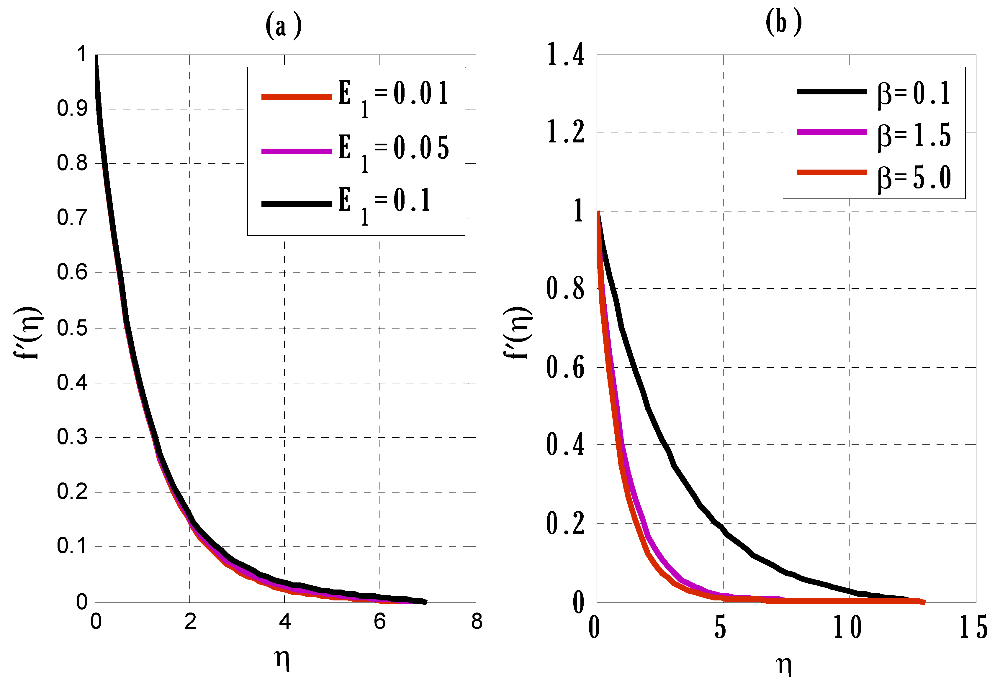
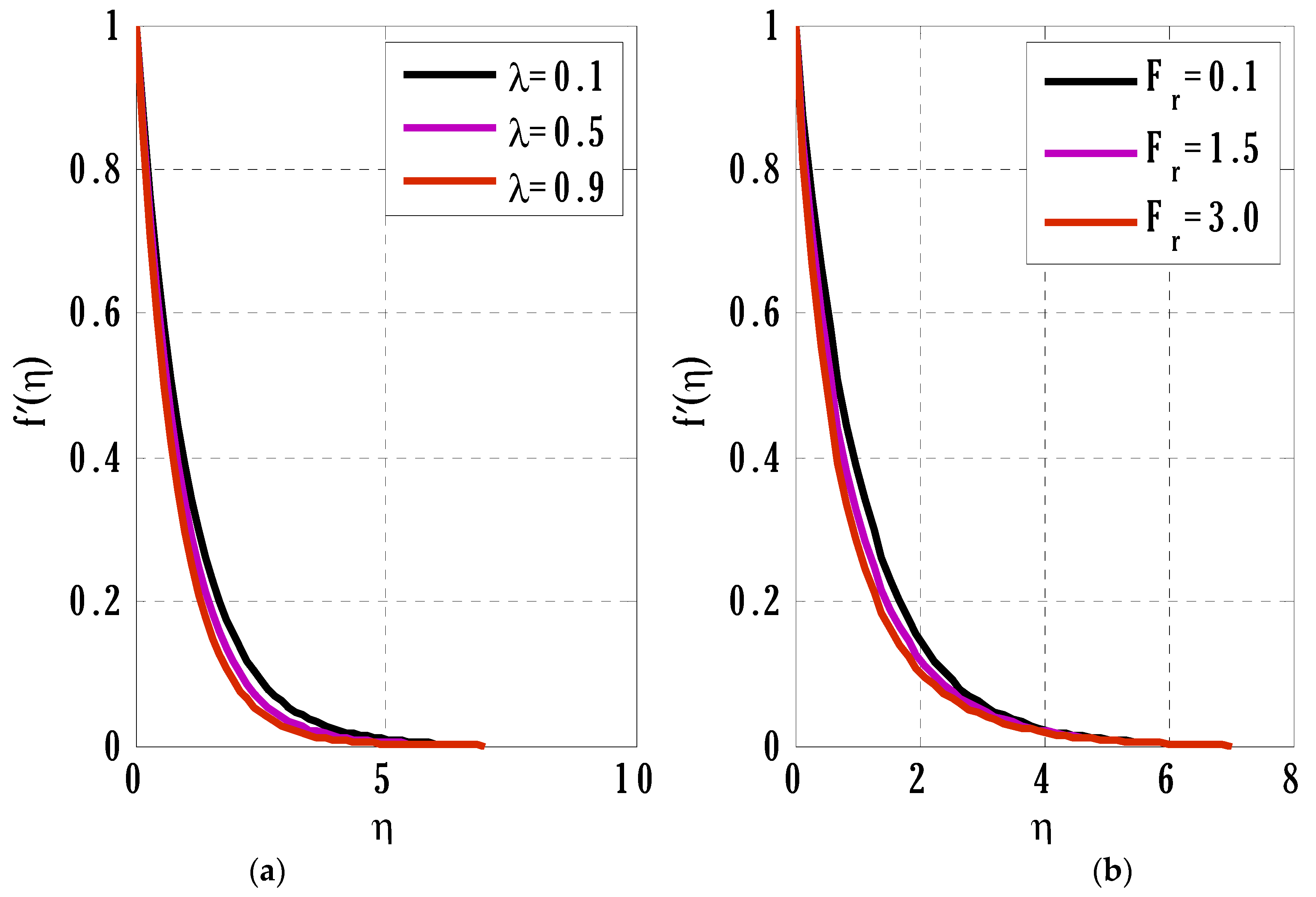
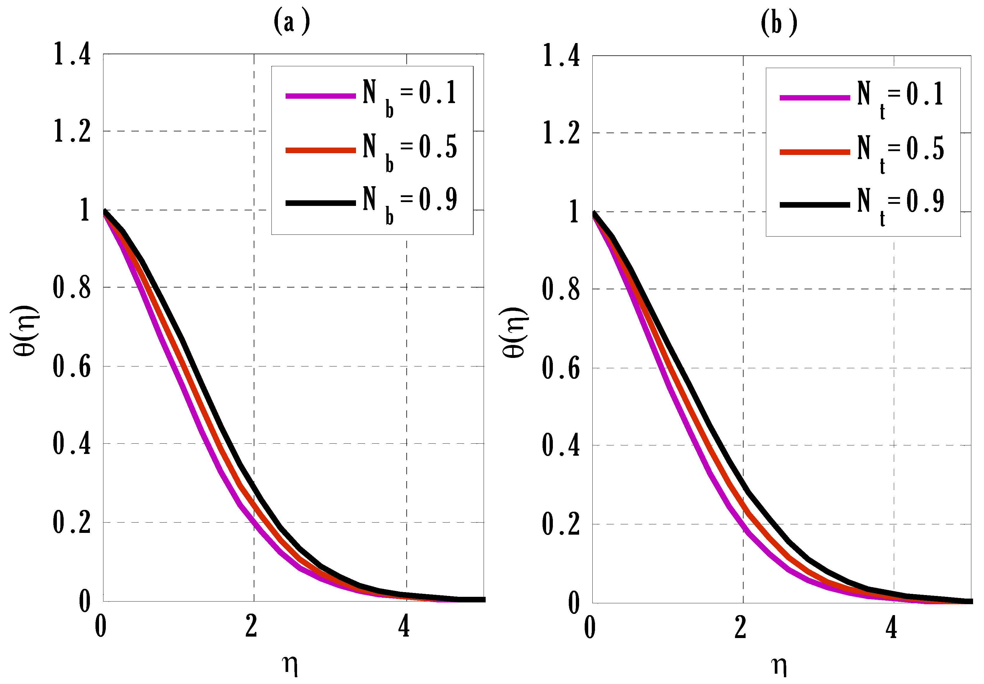
Figure 1 shows the impact of Casson and electric parameters on the velocity profile. The velocity profile declines and grows by enhancing the Casson and electric parameters. Because the increase in the Casson parameter decreases the diffusion coefficient, the diffusion process in the fluid slows down, resulting in a slower velocity profile. The behavior of the porosity parameter and inertia coefficient on the velocity profile is depicted in Figure 2. The velocity profile decays by growing porosity parameter and inertia coefficient values. Since, as the porosity parameter increases, either the viscosity of the fluid or the porosity of the medium increases, the flow velocity decreases in both cases. The decrease in the velocity profile caused by an increase in the inertia coefficient corresponds to an increase in the drag force that opposes the flow’s velocity. Figure 3 discusses the impact of Brownian motion and thermophoresis factors on the temperature profile. Temperature profile increases when Brownian motion and thermophoresis parameters increase in value. This is the case when the random movement of particles in the fluid increases, so hot particles of fluid spread in different locations of the fluid, leading to enhancement in the temperature profile. In addition, because of the augmentation in the thermophoresis parameter, thermophoresis force increases; due to this, hot force particles from the plate shift to their surroundings, and cold particles come closer to the plate, producing growth in the temperature profile.

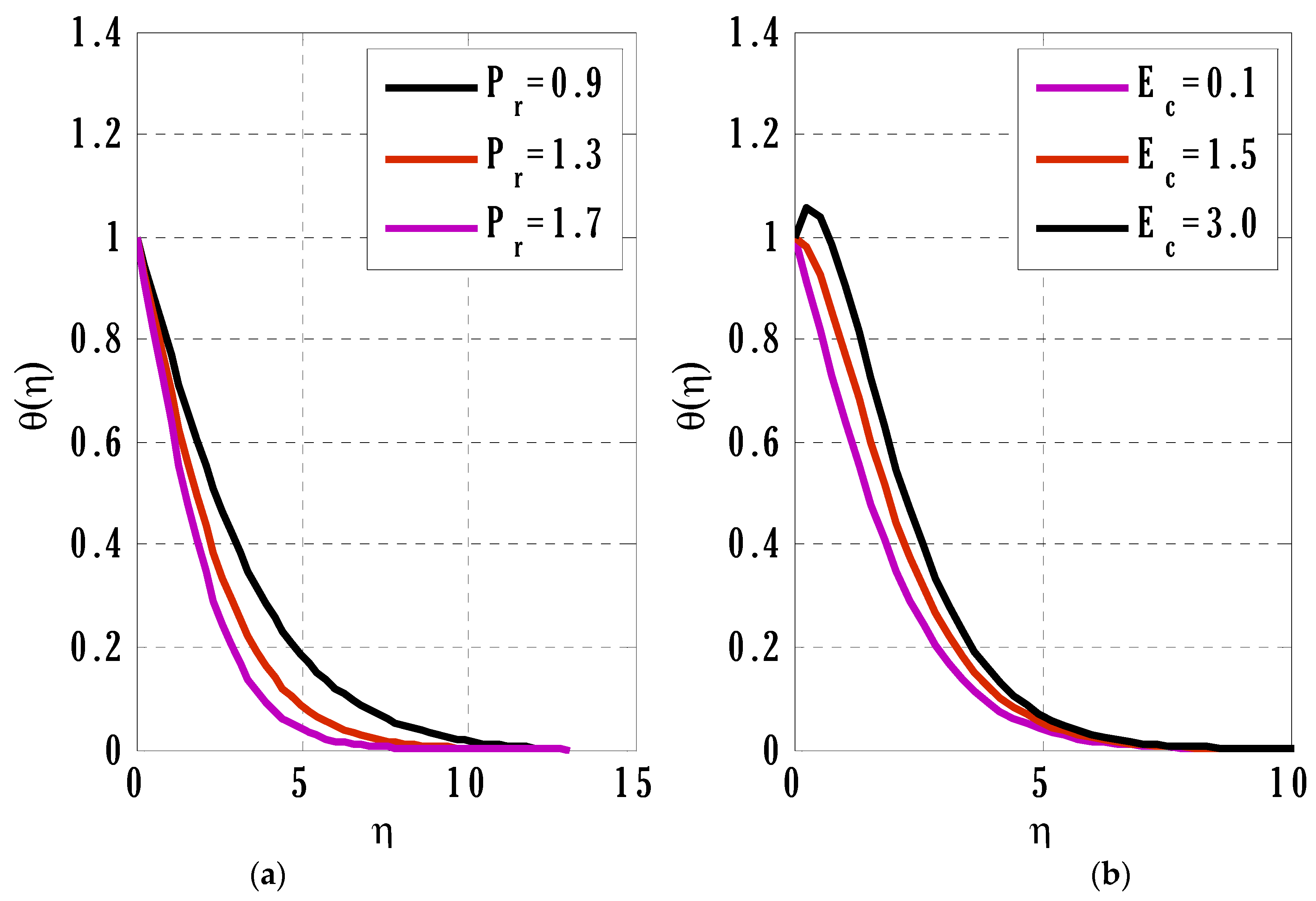
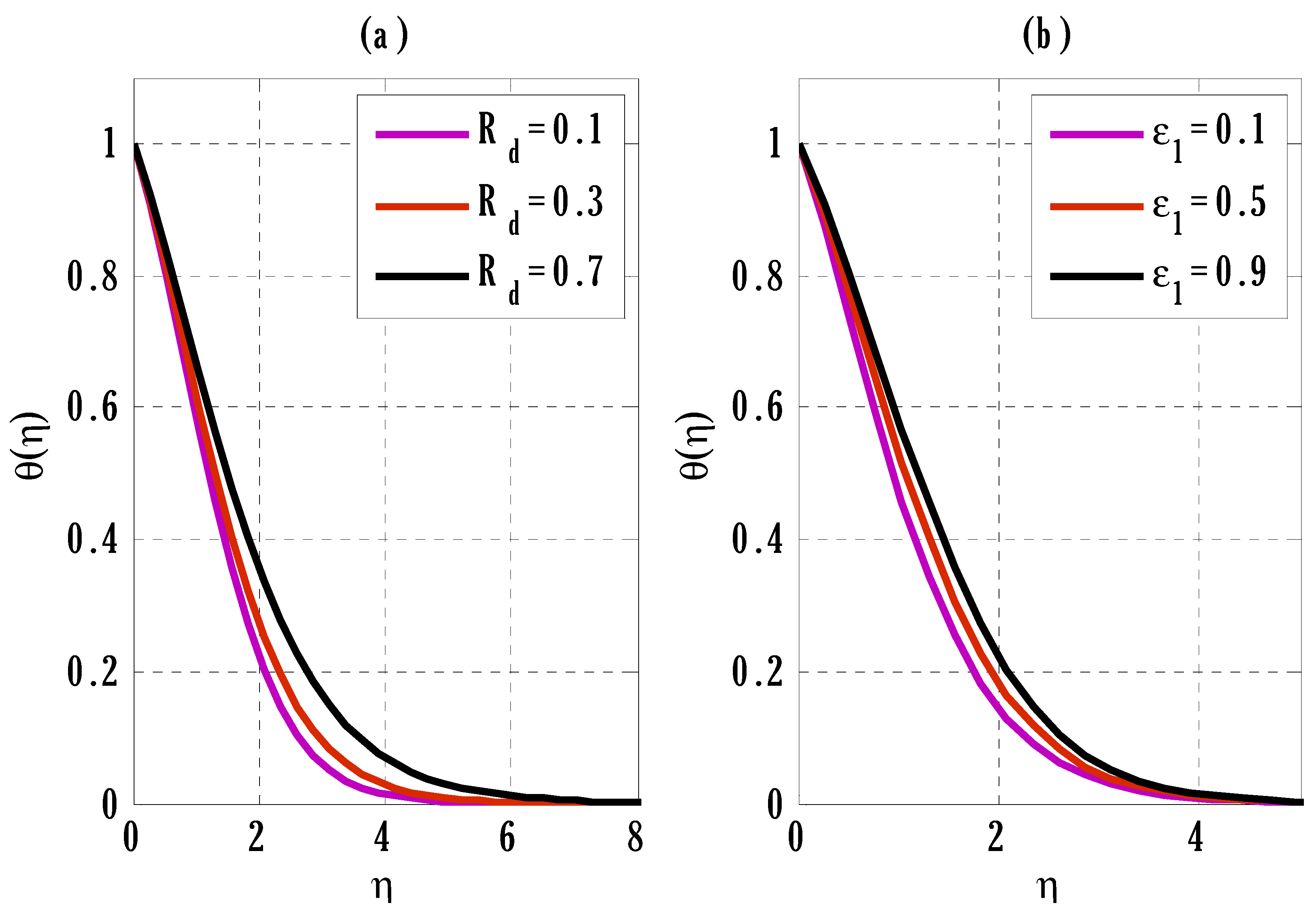
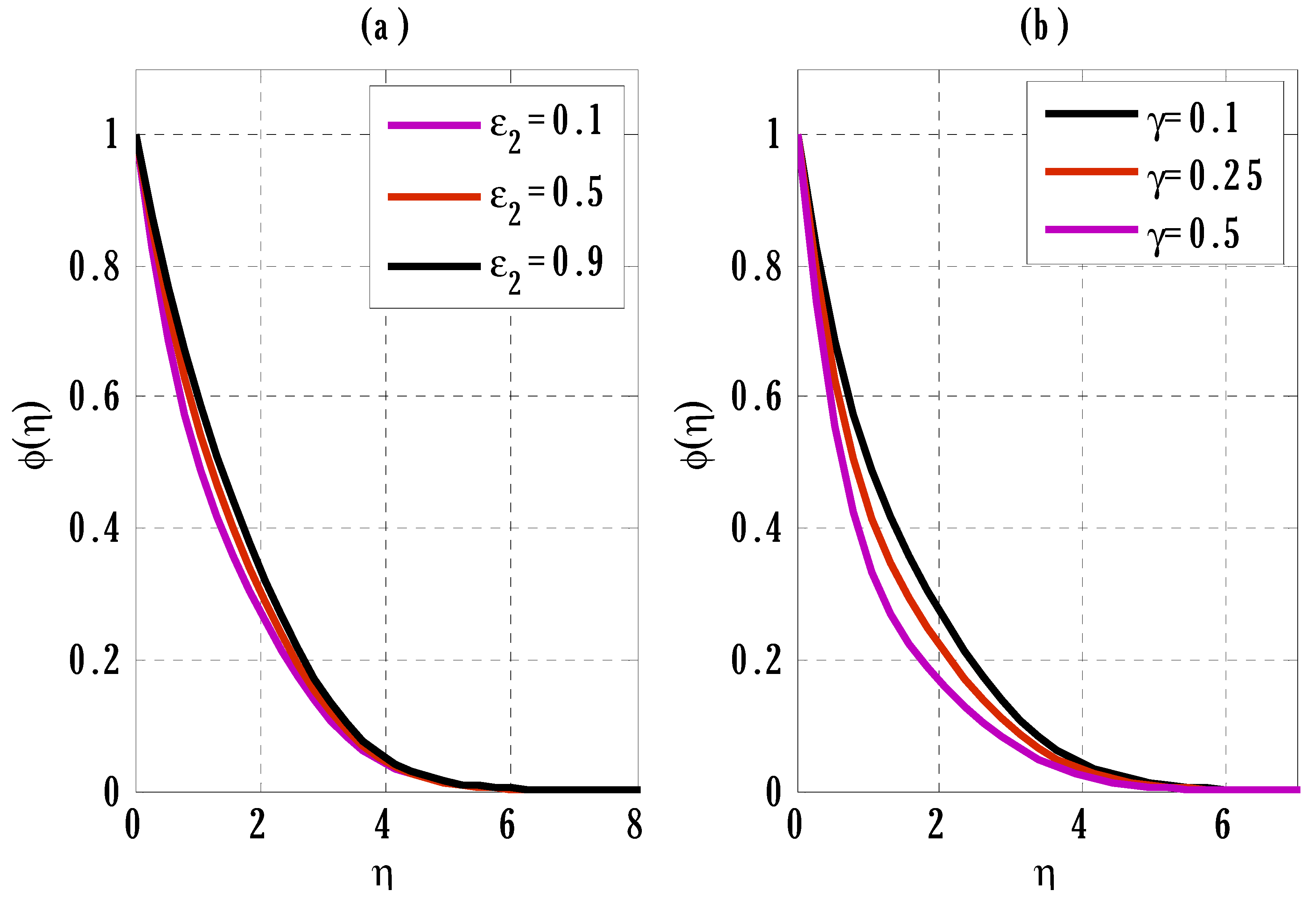
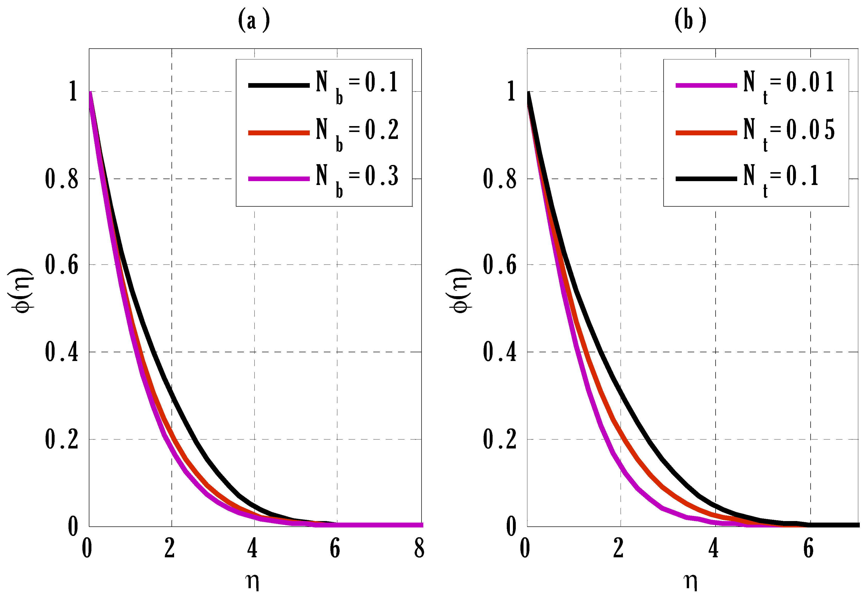
Figure 4 displays the temperature profile by varying the Prandtl and Eckert numbers. Temperature profile falloffs and develops by escalating the Prandtl and Eckert numbers, respectively. Since the Prandtl number and thermal diffusivity are inversely related, an increase in the Prandtl number leads to a decline in thermal diffusivity and a decrease in thermal conductivity, resulting in a temperature profile that falls off. The augmentation in the Eckert number yields progress in the friction of particles, so the temperature profile progresses. Figure 5 demonstrates the outcome of the temperature profile by a rising radiation parameter and a small parameter. The temperature profile rises by growing values of the radiation parameter and a small parameter. The escalation in temperature profile is the consequence of growing radiative flux due to the entrance of radiations into fluid and thermal conductivity augments by improving small parameters. Figure 6 shows the influence of small and reaction rate parameters in concentration profiles. The concentration profile rises and decays by enhancing a small parameter (in concentration) and reaction rate, respectively. The rise in the concentration profile due to a small parameter (in concentration) is the consequence of the growth of mass diffusivity. Figure 7 shows the effect of Brownian motion and thermophoresis parameters on the concentration profile. The concentration profile decays and rises by enhancing Brownian motion and thermophoresis parameters, respectively.

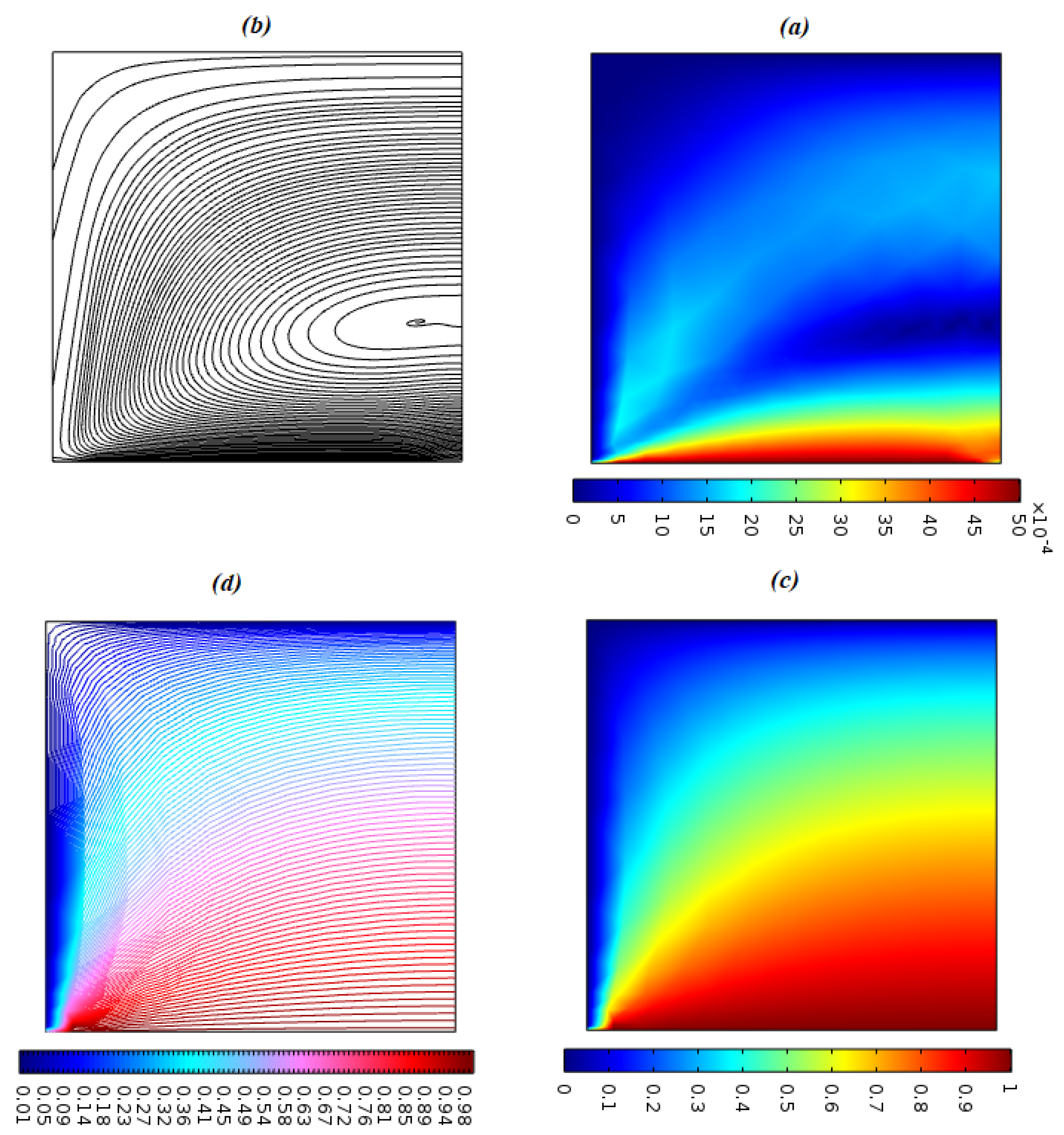
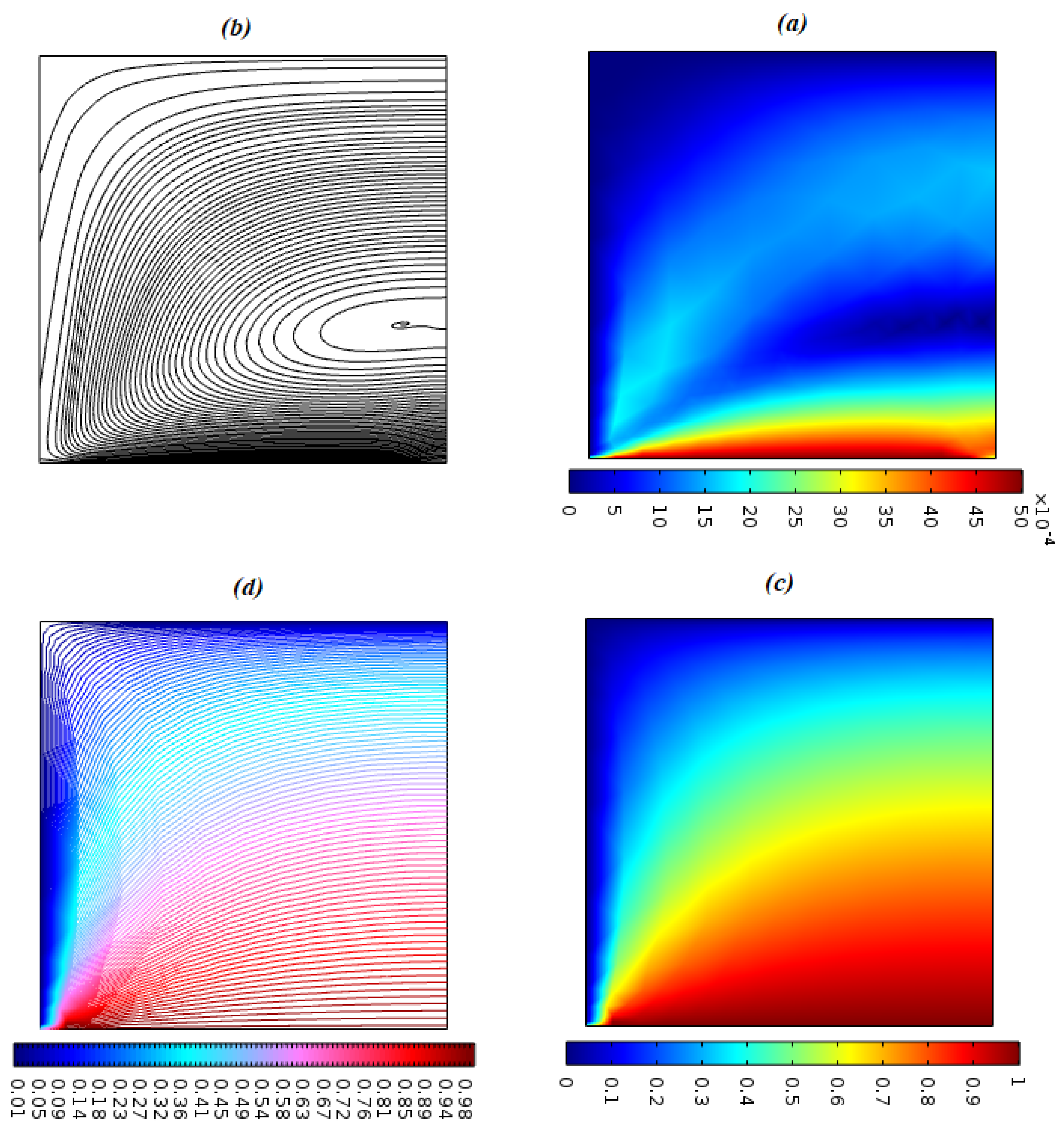
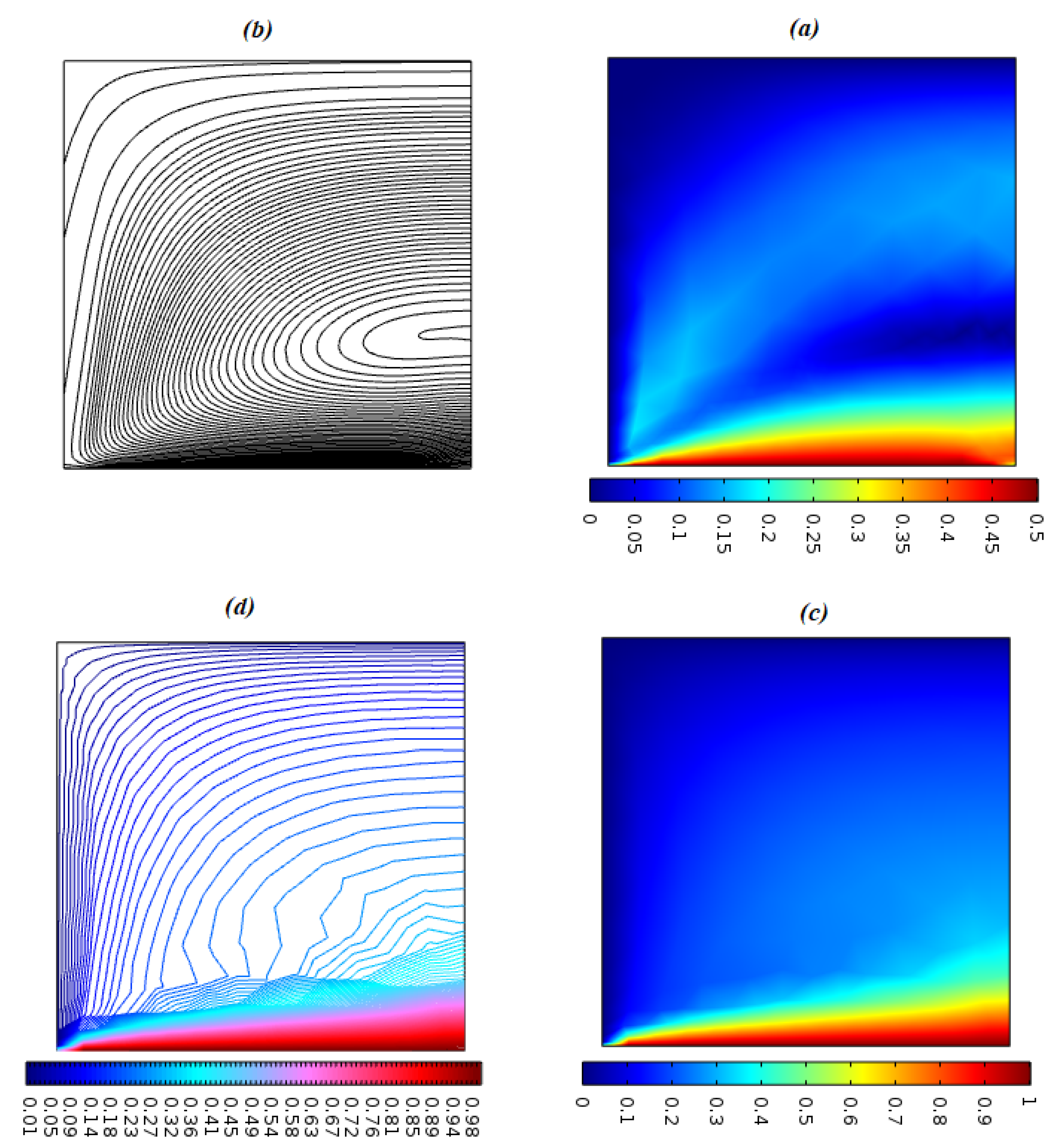
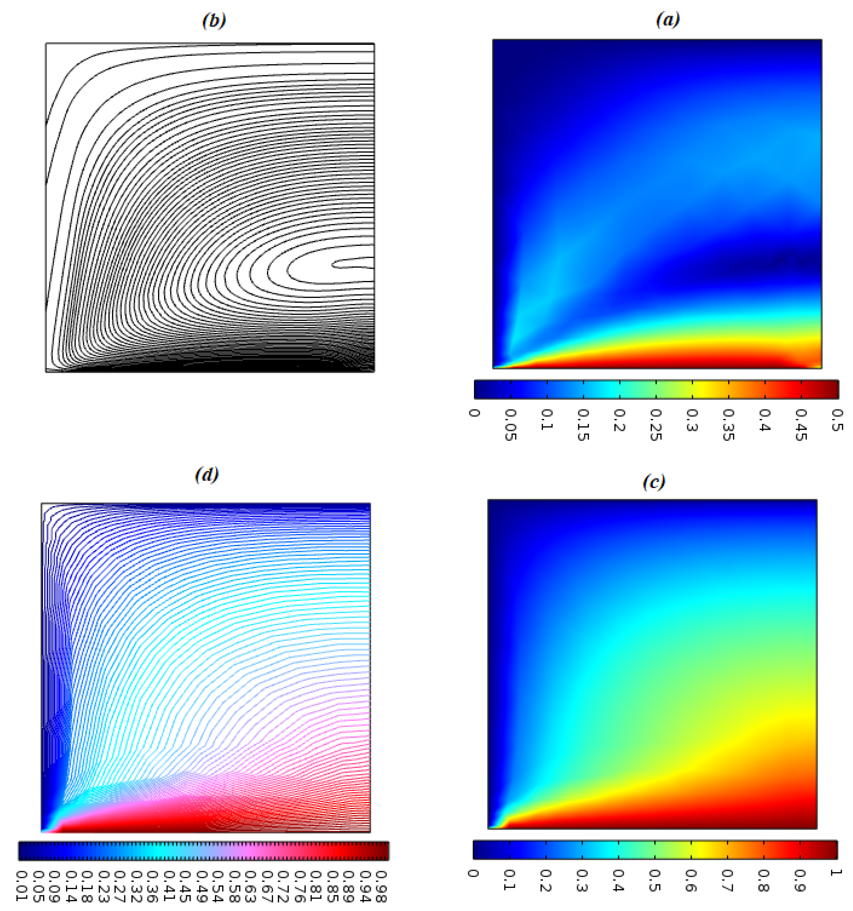
Figure 8, Figure 9, Figure 10 and Figure 11 are drawn using the modified finite element method software. The software uses partial differential equations for the heat transfer of electrical MHD Casson fluid flow over a moving sheet with the effects of radiations. The variation of different velocities of the sheet and thermal conductivity on velocity and temperature profile is displayed in Figure 8, Figure 9, Figure 10 and Figure 11.

Table 3. List of numerical values for the skin friction coefficient (excluding the Reynolds number) using $M=0.5$.

$\mathit{\lambda }$	${\mathit{F}}_{\mathit{r}}$	$\mathit{\beta }$	${\mathit{E}}_1$	${\mathit{R}}_{\mathit{e}}^{1/2}{\mathit{C}}_{\mathit{f}}$
				$\mathit{F}.\mathit{E}.\mathit{M}$	$\mathit{b}\mathit{v}\mathit{p}4\mathit{c}$
$0.1$	$0.1$	$0.5$	$0.01$	$2.24160$	$2.24163$
$0.5$				$2.48992$	$2.48997$
$0.1$	$0.4$			$2.36743$	$2.36747$
	$0.1$	$3$		$1.48549$	$1.48553$
		$0.5$	$0.05$	$2.21507$	$2.21510$

shows the numerical values of skin friction coefficient (excluding the Reynolds number) with varying porosity parameters, inertia coefficient, Casson parameter, and electric parameter. The skin friction coefficient grows by rising the porosity and inertia coefficient while it declines by enhancing the Casson and electric parameters.

Table 4. List the numerical values for the the local Nusselt number (excluding the Reynolds number) using $M=0.5, \lambda =0.1, F_r=0.1, S_c=1.5, E_1=0.05, \beta =0.5, {\epsilon }_2=0.1, \gamma =0.25$.

${\mathit{P}}_{\mathit{r}}$	${\mathit{E}}_{\mathit{c}}$	${\mathit{N}}_{\mathit{b}}$	${\mathit{N}}_{\mathit{t}}$	${\mathit{R}}_{\mathit{d}}$	${\mathit{\epsilon }}_1$	${\mathit{R}}_{\mathit{e}}^{-1/2}\mathit{N}{\mathit{u}}_{\mathit{x}}$
						$\mathit{F}.\mathit{E}.\mathit{M}$	$\mathit{b}\mathit{v}\mathit{p}4\mathit{c}$
$0.9$	$0.1$	$0.01$	$0.01$	$0.1$	$0.1$	$0.54979$	$0.54965$
$1.5$						$0.73162$	$0.73259$
$0.9$	$0.5$					$0.38035$	$diverges$
	$0.1$	$0.1$				$0.52511$	$0.52493$
		$0.01$	$0.1$			$0.53416$	$diverges$
			$0.01$	$0.5$		$0.67533$	$0.67461$
				$0.1$	$0.9$	$0.38936$	$0.38885$

shows the influence of the Prandtl number, Eckert number, Brownian and thermophoresis parameters, radiations parameter, and a small parameter. The local Nusselt number (excluding the Reynolds number) escalates by increasing the Prandtl number and radiation parameter. At the same time, it decays by raising the Eckert number, Brownian parameter, thermophoresis parameters, and a small parameter.

Table 5. List the numerical values for the local Sherwood number (excluding the Reynolds number) using $M=0.5, \lambda =0.1, F_r=0.1, S_c=1.5, E_1=0.05, \beta =0.5, {\epsilon }_2=0.1, \gamma =0.25$.

${\mathit{S}}_{\mathit{c}}$	${\mathit{N}}_{\mathit{b}}$	${\mathit{N}}_{\mathit{t}}$	${\mathit{\epsilon }}_2$	$\mathit{\gamma }$	${\mathit{R}}_{\mathit{e}}^{-1/2}\mathit{S}{\mathit{h}}_{\mathit{x}}$
					$\mathit{F}.\mathit{E}.\mathit{M}$	$\mathit{b}\mathit{v}\mathit{p}4\mathit{c}$
$0.9$	$0.01$	$0.01$	$0.1$	$0.1$	$0.52511$	$0.52543$
$1.5$					$0.75428$	$0.75454$
$0.9$	$0.1$				$0.61965$	$diverges$
	$0.01$	$0.1$			$-0.37128$	$diverges$
		$0.01$	$0.9$		$0.36318$	$diverges$
			$0.1$	$0.7$	$0.89306$	$0.89328$

shows the numerical values of the local Sherwood number (excluding Reynolds number) by varying Schmidt number, Brownian motion parameter, thermophoresis parameter, a small parameter (for concentration), and reaction rate parameter. The local Sherwood number rises by enhancing Schmidt number, Brownian motion parameter, and reaction rate parameter while it decays by growing the thermophoresis parameter and a small parameter (in concentration).

5. Conclusions

The modified finite element method has been adopted for solving the dimensionless equations that arise in the phenomenon of heat and mass transfer of non-Newtonian Casson fluid flow under the effects of viscous dissipation, thermal radiations, and chemical reaction. The linear polynomial interpolation has been considered in the modified finite element method. Some of the results have also been calculated with Matlab solver bvp4c, which can be used to solve boundary value problems. Briefly summarising the arguments:

• the modified finite element method converged for all parameters in this study, but Matlab solver $bvp4c$ could not converge for some of the results;
• velocity profile decayed by rising porosity parameter and inertia coefficient;
• Brownian motion and thermophoresis parameters increased, leading to a higher temperature profile.

In addition, nonlinear problems of a similar nature that arise in computational fluid dynamics can be quickly solved using the modified finite element method presented here. After this project is finished, further uses for the current approach can be suggested [47,48,49,50]. The suggested method is not only simple to implement, but it also solves a more general class of differential equations.

References

- Yu, W.; Xie, H.; Bao, D. Enhanced thermal conductivities of nanofluids containing graphene oxide nanosheets. Nanotechnology 2009, 21, 055705. [Google Scholar] [CrossRef] [PubMed]
- Reddy, J.R.; Sugunamma, V.; Sandeep, N. Impact of nonlinear radiation on 3D magneto hydrodynamic flow of methanol and kerosene based ferrofluids with temperature dependent viscosity. J. Mol. Liq. 2017, 236, 93–100. [Google Scholar] [CrossRef]
- Choi, S.U.; Eastman, J.A. Enhancing thermal conductivity of fluids with nanoparticles. In Proceedings of the International Mechanical Engineering Congress and Exhibition, San Francisco, CA, USA, 12–17 November 1995. ANL/MSD/CP-84938; CONF-951135-29 ON:DE96004174; TRN: 96:001707. [Google Scholar]
- Öztop, H.F.; Estellé, P.; Yan, W.M.; Al-Salem, K.; Orfi, J.; Mahian, O. A brief review of natural convection in enclosures under localized heating with and without nanofluids. Int. Commun. Heat Mass Transf. 2015, 60, 37–44. [Google Scholar] [CrossRef]
- Souayeh, B.; Reddy, M.G.; Sreenivasulu, P.; Poornima TM, I.M.; Rahimi-Gorji, M.; Alarifi, I.M. Comparative analysis on nonlinear radiative heat transfer on MHD Casson nanofluid past a thin needle. J. Mol. Liq. 2019, 284, 163–174. [Google Scholar] [CrossRef]
- Alwawi, F.A.; Alkasasbeh, H.T.; Rashad, A.M.; Idris, R. MHD natural convection of sodium alginate Casson nanofluid over a solid sphere. Results Phys. 2020, 16, 102818. [Google Scholar] [CrossRef]
- Saqib, M.; Ali, F.; Khan, I.; Sheikh, N.A.; Shafie, S.B. Convection in ethylene glycol-based molybdenum disulfide nanofluid. J. Therm. Anal. Calorim. 2019, 135, 523–532. [Google Scholar] [CrossRef]
- Miles, A.; Bessaïh, R. Heat transfer and entropy generation analysis of three-dimensional nanofluids flow in a cylindrical annulus filled with porous media. Int. Commun. Heat Mass Transf. 2021, 124, 105240. [Google Scholar] [CrossRef]
- Aglawe, K.R.; Yadav, R.K.; Thool, S.B. Preparation, applications and challenges of nanofluids in electronic cooling: A systematic review. Mater. Today Proc. 2021, 43, 366–372. [Google Scholar] [CrossRef]
- Tlili, I. Impact of thermal conductivity on the thermophysical properties and rheological behavior of nanofluid and hybrid nanofluid. Math. Sci. 2021, 1–9. [Google Scholar] [CrossRef]
- Archana, M.; Praveena, M.M.; Kumar, K.G.; Shehzad, S.A.; Ahmad, M. Unsteady squeezed Casson nanofluid flow by considering the slip condition and time-dependent magnetic field. Heat Transf. 2020, 49, 4907–4922. [Google Scholar] [CrossRef]
- Reddy, M.G.; Vijayakumari, P.; Sudharani, M.; Kumar, K.G. Quadratic convective heat transport of Casson nanoliquid over a contract cylinder: An unsteady case. BioNanoScience 2020, 10, 344–350. [Google Scholar] [CrossRef]
- Lokesh, H.J.; Gireesha, B.J.; Kumar, K.G. Characterization of chemical reaction on magnetohydrodynamics flow and nonlinear radiative heat transfer of Casson nanoparticles over an exponentially sheet. J. Nanofluids 2019, 8, 1260–1266. [Google Scholar] [CrossRef]
- Shehzad, S.; Hayat, T.; Alsaedi, A. Three-dimensional MHD flow of Casson fluid in porous medium with heat generation. J. Appl. Fluid Mech. 2016, 9, 215–223. [Google Scholar] [CrossRef]
- Durairaj, M.; Ramachandran, S.; Mehdi Rashidi, M. Heat generating/absorbing and chemically reacting Casson fluid flow over a vertical cone and flat plate saturated with non-Darcy porous medium. Int. J. Numer. Methods Heat Fluid Flow 2017, 27, 156–173. [Google Scholar] [CrossRef]
- Khan, A.; Khan, I.; Khan, A.; Shafie, S. Heat transfer analysis in MHD flow of Casson fluid over a vertical plate embedded in a porous medium with arbitrary wall shear stress. J. Porous Media 2018, 21, 739–748. [Google Scholar] [CrossRef]
- Imran, M.A.; Sarwar, S.; Imran, M. Effects of slip on free convection flow of Casson fluid over an oscillating vertical plate. Bound. Value Probl. 2016, 2016, 30. [Google Scholar] [CrossRef] [Green Version]
- Nawaz, M.; Naz, R.; Awais, M. Magneto hydrodynamic axisymmetric flow of Casson fluid with variable thermal conductivity and free stream. Alex. Eng. J. 2018, 57, 2043–2050. [Google Scholar] [CrossRef]
- Animasaun, I.L.; Adebile, E.A.; Fagbade, A.I. Casson fluid flow with variable thermo-physical property along exponentially stretching sheet with suction and exponentially decaying internal heat generation using the homotopy analysis method. J. Niger. Math. Soc. 2016, 35, 1–17. [Google Scholar] [CrossRef] [Green Version]
- Sheikh, N.A.; Ali, F.; Saqib, M.; Khan, I.; Jan, S.A.A.; Alshomrani, A.S.; Alghamdi, M.S. Comparison and analysis of the Atangana–Baleanu and Caputo–Fabrizio fractional derivatives for generalized Casson fluid model with heat generation and chemical reaction. Results Phys. 2017, 7, 789–800. [Google Scholar] [CrossRef]
- Imran, J.; Harff, P.; Parker, G. A numerical model of submarine debris flow with graphical user interface. Comput. Geosci. 2001, 27, 717–729. [Google Scholar] [CrossRef]
- Jeong, S.W. Determining the viscosity and yield surface of marine sediments using modified Bingham models. Geosci. J. 2013, 17, 241–247. [Google Scholar] [CrossRef]
- Kala, B.S. The numerical study of effects of Soret, Dufour and viscous dissipation parameters on steady MHD Casson fluid flow through non-Darcy porous media. Asian J. Chem. Sci. 2017, 2, 1–20. [Google Scholar] [CrossRef]
- Eldabe, N.T.M.; Moatimid, G.M.; Ali, H.S. Magneto hydrodynamic flow of non-Newtonian visco-elastic fluid through a porous medium near an accelerated plate. Can. J. Phys. 2003, 81, 1249–1269. [Google Scholar] [CrossRef]
- Sheikh, N.A.; Ching, D.L.C.; Khan, I.; Kumar, D.; Nisar, K.S. A new model of fractional Casson fluid based on generalized Fick’s and Fourier’s laws together with heat and mass transfer. Alex. Eng. J. 2020, 59, 2865–2876. [Google Scholar] [CrossRef]
- Qureshi, I.H.; Nawaz, M.; Abdel-Sattar, M.A.; Aly, S.; Awais, M. Numerical study of heat and mass transfer in MHD flow of nanofluid in a porous medium with Soret and Dufour effects. Heat Transf. 2021, 50, 4501–4515. [Google Scholar] [CrossRef]
- Saqib, M.; Khan, I.; Shafie, S.; Mohamad, A.Q. Shape effect on MHD flow of time fractional Ferro-Brinkman type nanofluid with ramped heating. Sci. Rep. 2021, 11, 3725. [Google Scholar] [CrossRef] [PubMed]
- Gireesha, B.J.; Kumar, K.G.; Krishnamurthy, M.R.; Manjunatha, S.; Rudraswamy, N.G. Impact of ohmic heating on MHD mixed convection flow of Casson fluid by considering cross diffusion effect. Nonlinear Eng. 2019, 8, 380–388. [Google Scholar] [CrossRef]
- Abdulaziz, O.; Noor, N.F.M.; Hashim, I. Homotopy analysis method for fully developed MHD micropolar fluid flow between vertical porous plates. Int. J. Numer. Meth. Eng. 2009, 78, 817–827. [Google Scholar] [CrossRef]
- Rizk, D.; Ullah, A.; Elattar, S.; Alharbi, K.A.M.; Sohail, M.; Khan, R.; Khan, A.; Mlaiki, N. Impact of the KKL correlation model on the activation of thermal energy for the hybrid nanofluid (GO+ZnO+Water) flow through permeable vertically rotating surface. Energies 2022, 15, 2872. [Google Scholar] [CrossRef]
- Suganya, S.; Muthtamilselvan, M.; Al-Amri, F.; Abdalla, B. An exact solution for unsteady free convection flow of chemically reacting Al2O3 − SiO2/water hybrid nanofluid. Proc. Inst. Mech. Eng. Part C J. Mech. Eng. Sci. 2021, 235, 3749–3763. [Google Scholar] [CrossRef]
- Rashid, U.; Abdeljawad, T.; Liang, H.; Iqbal, A.; Abbas, M.; Siddiqui, M.J. The shape effect of gold nanoparticles on squeezing nanofluid flow and heat transfer between parallel plates. Math. Probl. Eng. 2020, 2020, 9584854. [Google Scholar] [CrossRef]
- Zhang, X.; Pan, C.; Xu, Z. Effect of contact resistance on liquid metal MHD flows through circular pipes. Fusion Eng. Des. 2013, 88, 2228–2234. [Google Scholar] [CrossRef]
- Crane, L.J. Flow past a stretching plate. Z. Angew. Math. Phys. 1970, 21, 645–647. [Google Scholar] [CrossRef]
- Chiam, T.C. Stagnation point flow towards a stretching plate. J. Phys. Soc. Jpn. 1994, 63, 2443–2444. [Google Scholar] [CrossRef]
- Mahapatra, T.R.; Gupta, A.S. Magnetohydrodynamic stagnation-point flow towards a stretching sheet. Acta Mech. 2001, 152, 191–196. [Google Scholar] [CrossRef]
- Labropulu, F.; Li, D. Stagnation-point flow of a second grade fluid with slip. Int. J. Nonlin. Mech. 2008, 43, 941–947. [Google Scholar] [CrossRef]
- Ishak, A.; Nazar, R.; Amin, N.; Filip, D.; Pop, I. Mixed convection in the stagnation point flow towards a stretching vertical permeable sheet, Malaysian. J. Math. Sci. 2007, 2, 217–226. [Google Scholar]
- Hayat, T.; Nawaz, M. Unsteady stagnation point flow of viscous fluid caused by an impulsively rotating disk. J. Taiwan Inst. Chem. Eng. 2011, 42, 41–49. [Google Scholar] [CrossRef]
- Kasaeian, A.; Eshghi, A.T.; Sameti, M. A review on the applications of nanofluids in solar energy systems. Renew. Sustain. Energy Rev. 2015, 43, 584–598. [Google Scholar] [CrossRef]
- Wang, R.; Chen, T.; Qi, J.; Du, J.; Pan, G.; Huang, L. Investigation on the heat transfer enhancement by nanofluid under electric field considering electrophorestic and thermophoretic effect. Case Stud. Therm. Eng. 2021, 28, 101498. [Google Scholar] [CrossRef]
- Wang, G.; Zhang, Z.; Wang, R.; Zhu, Z. A Review on Heat Transfer of Nanofluids by Applied Electric Field or Magnetic Field. Nanomaterials 2020, 10, 2386. [Google Scholar] [CrossRef]
- Waqas, M.; Khan, W.A.; Asghar, Z. An improved double diffusion analysis of non-Newtonian chemically reactive fluid in frames of variables properties. Int. Commun. Heat Mass Transf. 2020, 115, 104524. [Google Scholar] [CrossRef]
- Naseem, F.; Shafiq, A.; Zhao, L.; Naseem, A. MHD biconvective flow of Powell eyring nanofluid over stretched sur-face. AIP Adv. 2017, 7, 065013. [Google Scholar] [CrossRef] [Green Version]
- Alsaedi, A.; Khan, M.I.; Farooq, M.; Gull, N.; Hayat, T. Magnetohydrodynamic (MHD) stratified bioconvective flow of nanofluid due to gyrotactic microorganisms. Adv. Powder Technol. 2017, 28, 288–298. [Google Scholar] [CrossRef]
- Nawaz, Y.; Arif, M.S. An effective modification of finite element method for heat and mass transfer of chemically reactive unsteady flow. Comput. Geosci. 2020, 24, 275–291. [Google Scholar] [CrossRef]
- Bibi, M.; Nawaz, Y.; Arif, M.S.; Abbasi, J.N.; Javed, U.; Nazeer, A. A finite difference method and effective modification of gradient descent optimization algorithm for MHD fluid flow over a linearly stretching surface. Comput. Mater. Contin. 2020, 62, 657–677. [Google Scholar]
- Arif, M.S.; Bibi, M.; Jhangir, A. Solution of algebraic lyapunov equation on positive-definite hermitian matrices by using extended Hamiltonian algorithm. Comput. Mater. Contin. 2018, 54, 181–195. [Google Scholar]
- Pasha, S.A.; Nawaz, Y.; Arif, M.S. A third-order accurate in time method for boundary layer flow problems. Appl. Numer. Math. 2021, 161, 13–26. [Google Scholar] [CrossRef]
- Nawaz, Y.; Arif, M.S. Modified class of explicit and enhanced stability region schemes: Application to mixed convection flow in a square cavity with a convective wall. Int. J. Numer. Methods Fluids 2021, 93, 1759–1787. [Google Scholar] [CrossRef]
Figure 1.
Variation of electric and Casson parameters on velocity profile using .
Figure 2.
Variation of porosity parameter and inertia coefficient on velocity profile using .
Figure 3.
Variation of Brownian motion and thermophoresis parameters on temperature profile using .
Figure 4.
Variation of Prandtl number and Eckert number on temperature profile using .
Figure 5.
Variation of radiation parameter and a small parameter (in thermal conductivity) on temperature profile using .
Figure 6.
Variation of a small parameter (in variable mass diffusivity) and reaction rate parameter on concentration profile using .
Figure 7.
Variation of Brownian motion and thermophoresis parameters on concentration profile using .
Figure 8.
Surface plot for velocity, streamlines, surface plot for temperature, isothermal contours using software with .
Figure 9.
Figure 10.
Figure 11.
Surface plot for velocity, streamlines surface plot for temperature, isothermal contours using software with .