HistoSSL: Self-Supervised Representation Learning for Classifying Histopathology Images

Abstract

The success of image classification depends on copious annotated images for training. Annotating histopathology images is costly and laborious. Although several successful self-supervised representation learning approaches have been introduced, they are still insufficient to consider the unique characteristics of histopathology images. In this work, we propose the novel histopathology-oriented self-supervised representation learning framework (HistoSSL) to efficiently extract representations from unlabeled histopathology images at three levels: global, cell, and stain. The model transfers remarkably to downstream tasks: colorectal tissue phenotyping on the NCTCRC dataset and breast cancer metastasis recognition on the CAMELYON16 dataset. HistoSSL achieved higher accuracies than state-of-the-art self-supervised learning approaches, which proved the robustness of the learned representations.

1. Introduction

In the past decade, deep neural network-based supervised learning has outperformed human experts in classifying histopathology images. However, such success depends on a large amount of annotated training data [1]. Unlike natural images, which can be annotated via crowd-sourcing, histopathology can only be annotated by proficient pathologists. To address this issue, several self-supervised representation learning methods have been introduced. Although these approaches have demonstrated decent performance on natural images, they are still insufficient to consider the unique characteristics of histopathology images. We hope to incorporate the domain knowledge of histopathology into the successful self-supervised learning approaches to train more robust representations for the downstream classification task.

Recently, contrastive learning has been widely studied as a promising method for learning image representations. Contrastive learning is based on the premise that the features of positive sample pairs correspond to each other, and the features between positive and negative samples are distinct. The quality of sampling plays a crucial role in contrastive learning. For natural images, researchers generate positive samples through stochastic combinations of random augmentations, and negative samples are other instances within the dataset [2,3,4,5,6]. These approaches are insufficient for histopathology images for two reasons: (1) positive samples generated by random augmentation are less challenging, and (2) negative samples are noisy [7]. Several approaches have been proposed to increase the quality of sampling for histopathology images [8,9]. However, they introduce additional data preprocessing, clustering, or top-k searching over a memory bank. Meanwhile, the unique characteristics of histopathology images are still insufficiently leveraged.

Histopathology images hold hierarchical information at different levels. Pathologists can discriminate global-level semantic information (e.g., tumor presence [1]) for an image with a size of around $256\times 256$ pixels under $20\times$ magnification. At the cell-level view, which is around $32\times 32$ pixels, fine-grained morphological features such as nuclear atypia and cell size can be discerned [10]. For natural images, one study [5] leveraged the “local–global” feature correspondence by using multi-crop training. For histopathology images, the authors of [11] pointed out that the Simple Contrastive Learning of Representations (SimCLR) framework [3] is able to distinguish aggressive small crops as positive samples. Therefore, we argue that correspondence exists for a histopathology image between its global-level and cell-level features.

Hematoxylin and eosin (H&E) staining has stood as the most commonly used staining protocol in medical examination since its development in 1876 [12]. Hematoxylin is a cationic compound that highlights basophilic cell structures (nuclei, rough endoplasmic reticula, and ribosomes) with blue stains. Meanwhile, eosin is anionic and stains acidophilic cell structures (cytoplasm and extracellular matrix) with pink color [13]. In addition to H&E, pathologists use diaminobenzidine (DAB) in immunohistochemistry (IHC) to highlight specific biomarkers (e.g., Ki-67 and HER2) in brown [14]. The basophilic, acidophilic, and IHC-specific structures are different views of the same tissue. We argue that feature correspondence exists between the tissue and each of its structures.

Motivated by the above discussion, we propose the Histopathology-Oriented Self-Supervised Learning Framework (HistoSSL) to learn salient representations by incorporating this histopathology domain knowledge. HistoSSL employs knowledge distillation [5] to learn from the correspondence between positive pairs and does not need negative samples. Unlike conventional self-supervised learning frameworks that only learn from global-level feature correspondence, HistoSSL further leverages the inherent cell-level and stain-level feature correspondence in histopathology images to generate meaningful and challenging positive pairs, encouraging the model to learn more robust and comprehensive representations. Our proposed framework is backbone-agnostic and has been tested on both convolutional neural networks (CNNs) and vision transformers (ViTs). We performed extensive experiments on the NCTCRC [15] and CAMELYON16 [16,17] datasets to demonstrate the effectiveness of our proposed framework.

Our main contributions are summarized below:

1.

We propose HistoSSL, a histopathology-oriented self-supervised learning framework to learn representations from unannotated images.

2.

By incorporating domain knowledge, HistoSSL leverages the cell-level and stain-level feature correspondence in histopathology images to learn more robust representations.

3.

The pre-trained model transfers remarkably to the downstream colorectal tissue phenotyping and breast cancer metastasis recognition task.

4.

HistoSSL achieved state-of-the-art accuracy compared with recent self-supervised representation learning approaches.

The rest of the article is organized as follows. Section 2 summarizes the related works, including generative, predictive, and contrastive self-supervised learning approaches for both natural and histopathology images. In Section 3, we describe the proposed method in detail, including the overall self-supervised knowledge-distillation approach to learn from global-level feature correspondence and how to generate meaningful positive samples for histopathology images from cell-level and stain-level feature correspondence. In Section 4, we introduce the datasets used and the evaluation protocols. Comparisons with other state-of-the-art methods and ablation studies are provided in Section 5.

2. Related Work

2.1. Self-Supervised Representation Learning for Natural Images

The goal of self-supervised representation learning is to learn discriminative feature representations from unannotated data [18]. Generally, self-supervised representation learning approaches for computer vision can be categorized into three paradigms: generative, predictive, and contrastive [19].

Generative self-supervised learning trains the network to learn a content generation task. Autoencoders are a series of generative tasks that aim to generate an approximate reconstruction of the input [20]. Several methods have been proposed to improve autoencoders, such as image inpainting [21] and cross-channel autoencoders [22]. Inspired by the success of self-supervised masked language model [23] learning on natural language processing (NLP), researchers have proposed the masked pixel method [24] and patch-based masked autoencoders (MAE) [25].

Predictive self-supervised learning defines classification pretext tasks that can work as surrogate supervision signals. Noroozi et al. proposed a jigsaw puzzle-solving pretext task by predicting the indices of the chosen permutations [26]. Gidaris et al. claimed that a model needs to understand the objects in the image before correctly predicting its rotation [27]. Therefore, they proposed an image rotation prediction task to learn image representations.

Contrastive learning frameworks learn representations by contrasting positive samples against negative samples in the representation space [3]. For a robust model, the representations of positive pairs are close, and the negative pairs are distinct. The positive samples can be generated from different random augmented views of the same image [2,3,18] or from the output of an autoregressive model [28]. Negative samples serve as regularizers to prevent the model from collapsing [29]. Experiments have shown that a large number of consistent negative samples results in better representations [2]. Therefore, several approaches have been proposed to improve negative sampling. In-batch sampling approaches use the other instances within a minibatch as the negative samples [3,18,30]. This approach has the best consistency, but the number of negative samples is restricted by the batch size. Therefore, large batch size is preferred. Other approaches decouple the number of negative samples from batch size by caching the embeddings of negative samples [2,6,31]. Specifically, to reduce the feature inconsistency caused by caching, Wu et al. introduced proximal regularization [31]. He et al. built the cache using a momentum encoder and a memory queue to improve feature consistency and to ensure the samples with the least consistency are removed first [2,6].

Contrastive learning can also be performed without negative samples, i.e., only based on the premise that the representations of positive pairs correspond to each other [4,5]. These two approaches use the mean-teacher method [32] to build a slow-moving teacher network to produce stable outputs for the online student network. In particular, Grill et al. introduced a prediction head on top of the student to avoid collapse and minimize the mean-square error between the online network’s prediction and the target [4]. Caron et al. formulated the training as a knowledge distillation process and introduced centering and sharpening operations to avoid collapse [5].

2.2. Self-Supervised Representation Learning for Histopathology Images

Since there exists a large domain discrepancy between histopathology images and natural images [33], the aforementioned self-supervised learning approaches designed and tested on natural images need to be re-evaluated for their applicability [11]. Recent works mainly focus on two aspects: (1) designing histopathology-specific pretext tasks and (2) improving existing self-supervised frameworks.

For generative self-supervised learning, researchers applied the colorization pretext task in histopathology-specific hematoxylin-eosin-DAB (HED) color space to build cross-stain autoencoders [34,35,36]. Other researchers improved the masked autoencoder with contrastive loss [37] and knowledge distillation [38].

For predictive self-supervised learning, the aforementioned “rotation prediction” method is not viable for histopathology images, since the objects in histopathology images (i.e., cells and extracellular structures) are not orientational [11]. Based on the finding that histopathology images scanned at different magnification levels can be discerned by the size and texture of their nuclei, Sahasrabudhe et al. proposed a magnification-level prediction task specially designed for histopathology images [39].

However, these handcrafted predictive and generative learning approaches only concentrate on ad hoc pretext tasks and thus lack generality [3]. Therefore, contrastive learning approaches which form the training objective on the fly [2] have attracted the attention of recent researchers. The proposed HistoSSL is a contrastive learning framework that generates positive views at the beginning of each training iteration. HistoSSL exploited the domain knowledge of histopathology images to generate positive views at three levels: global, cell, and stain.

For the application of contrastive self-supervised learning to histopathology images, recent research has focused on increasing the diversity of positive samples and reducing the noise of negative samples (i.e., false negative samples). One study [8] employed whole slide image (WSI) data preprocessing to mark spatially adjacent negative instances from the same histopathology slide as positive. However, spatially adjacent sampling could yield more false positives. Therefore, similarity-based sampling in the representation space was introduced. The authors of [8] also utilize clustering to mine positive samples. The authors of [7] performed top-k sorting over a large memory bank to mine similar samples and treat them as pseudo-positive samples. Apart from the above success, self-supervised contrastive learning for histopathology images is still an open problem, and there are issues that have not been sufficiently addressed:

1.

To reduce the noise of negative samples, the above approaches require WSI data preprocessing or similarity-based sampling, which involves additional computational and memory overheads.

2.

Since similarity-based sampling is performed in the representation space, their quality relies on the model’s representation ability. Meanwhile, the model’s representation ability highly depends on sampling quality, which forms a circular dependency.

3.

These pseudo-positive samples do not belong to the same instance but are visually similar instances within the dataset, which are less challenging and less meaningful.

HistoSSL differs from the above approaches in the following:

1.

By employing mean-teacher knowledge distillation to avoid collapse [5], HistoSSL does not need negative samples. There is no need to consider the quality of negative samples.

2.

HistoSSL uses global-level augmentation, cell-level cropping, and stain decomposition to generate positive views for histopathology images at the beginning of each forward pass. There is no need for additional WSI data preprocessing or similarity-based sampling.

3.

Based on the histopathology domain prior, positive samples are generated for each input image from global-, cell- and stain-level features; they are challenging and meaningful.

3. Method

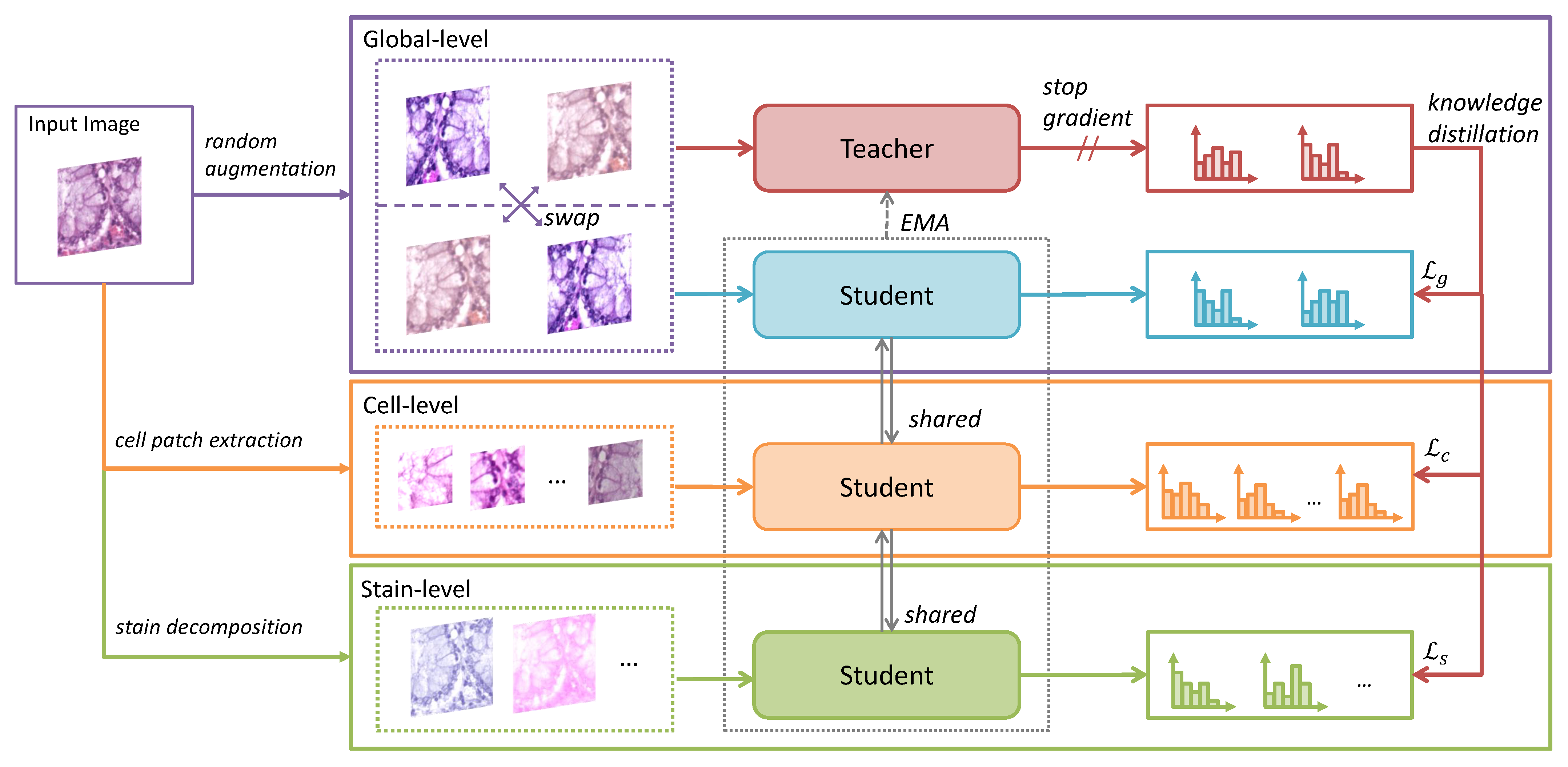
This section elaborates on the details of HistoSSL. As delineated in Figure 1, HistoSSL learns representations from feature correspondence by aligning the student distributions with the teacher distribution. Our framework leverages the feature correspondence in histopathology images and performs knowledge distillation at three levels: global-, cell-, and stain-level, encouraging the network to learn more robust representations. More details are discussed next.

3.1. Learning from Global-Level Feature Correspondence

The global-level feature is the augmentation-invariant representation of a given image. Global-level feature correspondence serves as a fundamental part of self-supervised learning frameworks [2,3,4,5,6]; i.e., for an input image, the representations of its different augmented views correspond to each other. Specifically, we use the knowledge-distillation loss [5] as the metric for the feature correspondence.

Take the student network S parameterized by ${\theta }_s$ and the teacher network T parameterized by ${\theta }_t$ with the same structure. For an image $\mathit{x}\in {\mathbb{R}}^{H\times W\times 3}$, two random augmented views ${\mathit{x}}_1\in {\mathbb{R}}^{H\times W\times 3}$ and ${\mathit{x}}_2\in {\mathbb{R}}^{H\times W\times 3}$ are sent to the student and teacher, respectively. The prediction of the student network is a K-dim probability distribution denoted as $p^S\left({\mathit{x}}_1\right)=softmax(S\left({\mathit{x}}_1\right)/{\tau }_s)$, where ${\tau }_s>0$ is the temperature hyper-parameter that controls the sharpness of $p^S$. Similarly, the teacher outputs a K-dim distribution $p^T\left({\mathit{x}}_2\right)$.

The augmentation-invariant representations are learned by minimizing the distance between $p^S$ and $p^T$. We define the loss function as:

$${\mathcal{L}}_g=H\left(p^T\left({\mathit{x}}_2\right),p^S\left({\mathit{x}}_1\right)\right)$$

(1)

where $H(·,·)$ refers to cross-entropy loss. By swapping $x_1$ with $x_2$, we can define a symmetrized loss as:

$${\mathcal{L}}_g=H\left(p^T\left({\mathit{x}}_1\right),p^S\left({\mathit{x}}_2\right)\right)+H\left(p^T\left({\mathit{x}}_2\right),p^S\left({\mathit{x}}_1\right)\right)$$

(2)

The parameters of the student network ${\theta }_s$ are updated by minimizing ${\mathcal{L}}_g$ using gradient descent. Moreover, the parameters of the teacher are updated by an exponential momentum-averaged mean-teacher paradigm [32]:

$${\theta }_t\leftarrow m{\theta }_t+(1-m){\theta }_s$$

(3)

3.2. Learning from Cell-Level Feature Correspondence

As discussed in Section 1, since histopathology images hold hierarchical information at different fields of view, we argue that feature correspondence exists for a histopathology image between its global-level view and cell-level views. Therefore, for an input image x, we can extract n cell-level augmented patches $x_j^{\prime }$. This operation is an improved version of the multi-crop training [5] by cropping and augmenting patches that are small enough to capture cell-level views.

We put these patches into the student network, generating a series of student distributions:

$$p^S\left(x_j^{\prime }\right)=softmax\left(S\left({\mathit{x}}_j^{\prime }\right)/{\tau }_s\right)$$

(4)

where $j\in [1,n]$. It is worth noticing that to ensure the stability [4] of the training target (i.e., teacher distribution), we do not put cell-level patches into the teacher network [5]. Accordingly, we perform knowledge distillation by minimizing the following loss:

$${\mathcal{L}}_c=\sum _{i=1}^2\sum _{j=1}^{n}H\left(p^T\left({\mathit{x}}_i\right),p^S\left({\mathit{x}}_j^{\prime }\right)\right)$$

(5)

3.3. Learning from Stain-Level Feature Correspondence

Different stains used in histopathology imaging highlight different cellular and extracellular structures. Since histopathology slides are thin and transparent to allow light to pass through, these different stains with known absorption spectra can overlap, affecting the RGB value in a non-linear way. In HistoSSL, we employ color deconvolution to decompose histopathology images into separated hematoxylin, eosin, and diaminobenzidine stains that represent basophilic, acidophilic, and IHC-specific structures. These structures are different views of the same tissue. We argue that feature correspondence exists between the tissue and each of its structures. Therefore, our HistSSL treats the separated stains as positive samples. To the best of our knowledge, this is the first attempt at utilizing stain decomposition to generate meaningful positive samples in self-supervised contrastive learning.

Histopathology imaging employs RGB sensors to capture and quantify light passed through tissue slides. The value for each of the RGB channels represents the brightness:

$$r=\frac{T_r}{I_r},g=\frac{T_g}{I_g},b=\frac{T_b}{I_b}$$

(6)

where I is the incident light and T is the transmitted light. For each RGB channel, the light transmitted through the tissue slide with the amount of stain A and absorption factor C is defined by the Beer–Lambert Law [40]:

$$T=I·exp(-AC).$$

(7)

In histopathology imaging, there are three types of stains: hematoxylin, eosin, and diaminobenzidine with corresponding amounts: h, e, and d; and absorption factors: $C_h$, $C_e$, and $C_d$. We have:

$$AC=h{C}_h+e{C}_e+d{C}_d.$$

(8)

Therefore, we have:

$$T=I·exp(-h{C}_h-e{C}_e-d{C}_d).$$

(9)

Hence, the relation between RGB and HED values can be expressed by the transformation matrix described in Equation (10):

$$\begin{array}{cc}\hfill \left[\begin{array}{ccc}\hfill -logr\hfill & \hfill -logg\hfill & \hfill -logb\hfill \end{array}\right]& \hfill =\left[\begin{array}{ccc}\hfill h\hfill & \hfill e\hfill & \hfill d\hfill \end{array}\right]\left[\begin{array}{c}\hfill C_{hr},C_{hg},C_{hb}\hfill \\ \hfill C_{er},C_{eg},C_{eb}\hfill \\ \hfill C_{dr},C_{dg},C_{db}\hfill \end{array}\right]\hfill \\ \hfill & \hfill =\left[\begin{array}{ccc}\hfill h\hfill & \hfill e\hfill & \hfill d\hfill \end{array}\right]\mathbf{M}\hfill \end{array}$$

(10)

where $\mathbf{M}$ here is called the normalized optical density (OD) matrix [14].

Based on the above discussions, for each pixel in the input image, we perform the color deconvolution [14] described in Equation (11) to get the values of hematoxylin, eosin, and diaminobenzidine.

$$\begin{array}{cc}\hfill \left[\begin{array}{ccc}h\hfill & e\hfill & d\hfill \end{array}\right]& =\left[\begin{array}{ccc}-logr\hfill & -logg\hfill & -logb\hfill \end{array}\right]{\mathbf{M}}^{-1}\hfill \\ \hfill & =\left[\begin{array}{ccc}-logr\hfill & -logg\hfill & -logb\hfill \end{array}\right]\left[\begin{array}{ccc}1.88& -0.07& -0.60\\ -1.02& 1.13& -0.48\\ -0.55& -0.13& 1.57\end{array}\right]\hfill \end{array}$$

(11)

For each type of separated stain, we convert its value back to the RGB color space independently:

$$\left\{\begin{array}{cc}\hfill {\mathit{x}}_h& \hfill =exp\left(-\left[\begin{array}{ccc}h& 0& 0\end{array}\right]\mathbf{M}\right)\hfill \\ \hfill {\mathit{x}}_e& \hfill =exp\left(-\left[\begin{array}{ccc}0& e& 0\end{array}\right]\mathbf{M}\right)\hfill \\ \hfill {\mathit{x}}_d& \hfill =exp\left(-\left[\begin{array}{ccc}0& 0& d\end{array}\right]\mathbf{M}\right)\hfill \end{array}\right.$$

(12)

where ${\mathit{x}}_h\in {\mathbb{R}}^{H\times W\times 3}$, ${\mathit{x}}_e\in {\mathbb{R}}^{H\times W\times 3}$, and ${\mathit{x}}_d\in {\mathbb{R}}^{H\times W\times 3}$ are the decomposed hematoxylin, eosin, and diaminobenzidine stains. We omitted the height H and width W dimensions in the above derivations for brevity. Similarly to Section 3.2, we put these separated stains in the student network and minimize the knowledge distillation loss:

$$\begin{array}{cc}\hfill {\mathcal{L}}_s& \hfill =\mathbb{I}\left(h\right)·\sum _{i=1}^{2}H\left(p^T\left({\mathit{x}}_i\right),p^S\left({\mathit{x}}_h\right)\right)\hfill \\ \hfill & \hfill +\mathbb{I}\left(e\right)·\sum _{i=1}^{2}H\left(p^T\left({\mathit{x}}_i\right),p^S\left({\mathit{x}}_e\right)\right)\hfill \\ \hfill & \hfill +\mathbb{I}\left(d\right)·\sum _{i=1}^{2}H\left(p^T\left({\mathit{x}}_i\right),p^S\left({\mathit{x}}_d\right)\right)\hfill \end{array}$$

(13)

where $\mathbb{I}\left(·\right)$ is the function indicating if the specified stains were used, e.g., $\mathbb{I}\left(d\right)$ is 0 for H&E stained images.

The overall training objective is to minimize the losses from the global level, cell level, and stain level, which are defined in Equations (2), (5) and (13). Since ${\mathcal{L}}_g$, ${\mathcal{L}}_c$, and ${\mathcal{L}}_s$ are all summations of cross-entropy losses, the final training loss is the average of all the summation terms.

$$\mathcal{L}=\frac{{\mathcal{L}}_g+{\mathcal{L}}_c+{\mathcal{L}}_s}{2\times [1+n+\mathbb{I}(h)+\mathbb{I}(e)+\mathbb{I}(d\left)\right]}$$

(14)

where n is the number of cell-level patches discussed in Section 3.2.

3.4. Model Architecture

As illustrated in Figure 2, the teacher and student models share the same architecture, which consists of a backbone and a header. The backbone is a function $f:{\mathbb{R}}^{H\times W\times 3}\to {\mathbb{R}}^F$ that takes an $H\times W\times 3$ sized image as the input and outputs a F-dim vector as its representation. The head is a learnable non-linear transformation between the representation and the K-dim probability space where to perform knowledge distillation [5]. The head is discarded after training, we use the trained backbone for downstream recognition tasks.

The backbone can be a ResNet [41] without the last fully connected layer or a vision transformer [42] without a classification head. As described in Section 3.2, the cell-level patches have a smaller size than the original image. To properly perform contrastive learning, the backbone needs to generate a fixed F-dim vector from images with different sizes.

ResNet-based backbones are fully convolutional and thus can handle variable input sizes. By adding a global average pooling layer after the residual blocks, the dimensions of the output vector only depend on the number of channels of the last convolution layer.

Vision transformers, on the other hand, leverage a patch embedding layer to convert 2D images into a sequence of tokens. A learnable positional encoding is added to the flattened tokens to preserve their spatial relations. A [CLS] token is prepended to the token sequences to capture the image representation through the multi-head self-attention (MHSA) mechanism. To handle variable input sizes, we interpolate the positional embedding at the beginning of each forward pass to match the number of tokens, which is illustrated in Figure 3. The output dimension of the ViT-based backbone is the size of [CLS] token of the last ViT block, which is independent of the input size.

The head starts with a 3-layer MLP with GELU activations [5], following an L2 normalization layer normalizing the output of the MLP onto the surface of a 256-dim unit sphere. The last linear layer outputs K-dim logits, and softmax projects these logits from ${\mathbb{R}}^K$ onto the probability simplex. We evaluated the impact of different values of K, which is the model’s output distribution dimension. The results are in Section 5.5.2.

4. Experiments

In this section, we first introduce the datasets used in our study. Then, we describe the setup of the experiments and the evaluation metrics.

4.1. Datasets

Our proposed framework was evaluated on two tasks: colorectal tissue phenotyping on the NCTCRC dataset [15] and breast cancer metastasis recognition on the CAMELYON16 dataset [16]. We chose these two tasks to cover both binary and multi-class classification tasks. From the medical perspective, these two tasks cover the diagnosis of both in situ and metastatic carcinoma.

4.1.1. NCTCRC Dataset

A colonoscopy is an effective way to screen for colorectal cancer. For polyps and hyperplastic tissue seen under endoscopy, a pathological biopsy is required to clarify its nature. Pathologists need to search a large number of tissue specimens for tiny lesions. To advance computer-aided colorectal cancer diagnosis research, Kather et al. published the NCTCRC dataset [15] in 2018. The NCTCRC dataset contains $107,180$ non-overlapping histopathology image tiles extracted from H&E stained slides in nine classes. Each tile has $224\times 224$ resolution, representing a 112 $\mathsf{\mu }\mathrm{m}\times$ 112 $\mathsf{\mu }\mathrm{m}$ tissue area. The dataset includes two subsets: NCT-CRC-HE-100K for self-supervised pre-training and CRC-VAL-HE-7K for evaluation. Details are shown in

Table 1. The organization of the NCTCRC dataset [15].

Class	Diagnosis	100 K for Pre-Training	7 K for Evaluation
ADI	adipose	10,407	1338
BACK	background	10,566	847
DEB	debris	11,512	339
LYM	lymphocytes	11,557	634
MUC	mucus	8896	1035
MUS	smooth muscle	13,536	592
NORM	normal colon mucosa	8763	741
STR	cancer-associated stroma	10,446	421
TUM	colorectal adenocarcinoma epithelium	14,317	1233
Total		100,000	7180

.

4.1.2. CAMELYON16 Dataset

Lymph-node metastasis is one of the most important prognostic factors for breast cancer [17]. CAMELYON16 is a publicly available dataset composed of 398 annotated slides (the dataset contains 399 slides in total; slide test_114 is not annotated) for detecting breast cancer metastasis in sentinel lymph nodes [16]. Slides are categorized into two classes: normal and tumor. Each slide has a size of around $100,000\times 100,000$ pixels. For tumor slides, the pixel-level tumor annotations are provided in XML format. As shown in

Table 2. Details of the CAMELYON16 dataset [16,17].

Class	Train Slides	Test Slides	Train Tiles	Test Tiles
Normal	159	80	200,000	50,000
Tumor	111	48	200,000	50,000
Total	270	128	400,000	100,000

, we employed OpenSlide [43] to randomly extract $500,000$ $256\times 256$ sized non-overlapping tiles from these slides to construct the train set and test set with balanced distributions between the two classes. (Early researchers use the word “patch” to refer to the small images extracted from the slides. Here we use the word “tile” to avoid confusion with the concept “patch” in vision transformers.)

4.2. Experimental Setup

A set of experiments were conducted in this study. First, we built the teacher and the student model by adding a head after the backbone, as described in Section 3.4. Then, we performed self-supervised pre-training on the unannotated train set. After pre-training, we discarded the head and evaluate the backbone on downstream tasks using k-nearest neighbor (k-NN) and linear probing protocol. All the experiments were implemented in PyTorch [44] on a server equipped with 2 Intel Xeon E5-2643 V4 CPUs, 128 GB RAM, and 4 NVIDIA Titan V GPUs with 12GB memory.

4.2.1. Self-Supervised Pre-Training

We performed experiments on various backbones, including both ConvNets and vision transformers [42]. The detailed comparison of different backbones is in Section 5.4. For ResNet-50 and ViT-T/16 backbones, the batch size per GPU was set to 32. We halved the batch size when training larger models and used mixed precision with gradient scaling to reduce the GPU memory consumption. A detailed summary of the hyper-parameters in our experiment is listed in

Table 3. Summary of the hyper-parameters in our self-supervised pre-training experiment.

Name	Value	Detail
epochs	100
optimizer	AdamW
batch size	128	32 per GPU × 4 GPUs
learning rate (LR)	0.00025	when batch size = 128
lr warmup	10 epochs	linear warmup
LR scheduler	cosine decay	to 0.000001
weight decay	cosine schedule	from 0.04 to 0.4
teacher temperature	0.04
student temperature	0.1
Mean-Teacher momentum	cosine schedule	from 0.997 to 1

.

We used a stochastic combination of random augmentations to generate global-level and cell-level views for the given images.

Table 4. Details of the random augmentations used to generate global-level and cell-level views.

Method	Parameters
Global-level cropping	area scale $\in [0.4,1]$
Cell-level patch extraction	n = 8, area scale $\in [0.01,0.2]$
Random color jitter	p = 0.8, brightness = 0.4, contrast = 0.4, saturation = 0.2, hue = 0.1
Random grayscale	p = 0.2
Random gaussian blur	p = 0.5, radius $\in [0.1,2]$

summarizes the details of the random augmentations and cell-level patch extraction.

4.2.2. k-NN Evaluation

As the name suggests, k-NN classifiers predict a given sample by voting its top-k nearest neighbors. Therefore, the k-NN classifier has only one hyper-parameter, k, and does not have an explicit learning process. Compared with the linear evaluation introduced in Section 4.2.3, the accuracy of k-NN is not affected by the randomness introduced in the neural network training, which makes it suitable for evaluating the representation ability of the pre-trained backbone. For self-supervised learning, we used the pre-trained backbone to embed both the training data and the testing data into the representation space and perform k-NN classification. The hyper-parameter k was set to 20 empirically [5] We also performed experiments to search for the value of k, as discussed in Section 5.5.1.

4.2.3. Linear Evaluation

Another widely used evaluation protocol for self-supervised learning is linear probing. We froze the parameters of the backbone and trained a linear classifier $g:{\mathbb{R}}^F\to {\mathbb{R}}^C$ on the top of the backbone, where C is the number of classes. We used an SGD optimizer with momentum $=0.9$ and no weight decay. A cosine-annealing learning rate scheduler decays the learning rate from 0.0005 to 0 in 20 epochs. We employed early-stopping scheduling, since linear probing has only one layer of trainable parameters and converges very fast.

4.3. Evaluation Metrics

Given a testing set D containing N samples:

$$D=\{({\mathit{x}}_1,y_1),({\mathit{x}}_2,y_2),\cdots ,({\mathit{x}}_N,y_N)\}$$

(15)

where $y_i\in \mathcal{Y}$ is the label of sample ${\mathit{x}}_i\in \mathcal{X}$. We evaluated classifier $f:\mathcal{X}\to \mathcal{Y}$ by calculating its accuracy:

$$Accuracy=\frac{1}{N}\sum _{i=1}^N\mathbb{I}\left(f\left({\mathit{x}}_i\right)=y_i\right).$$

(16)

We also report other common classification metrics: sensitivity, specificity, and area under the receiver operating characteristic curve (AUC). For the confusion matrix of a binary classifier, we have the number of true positives (TP), false positives (FP), true negatives (TN), and false negatives (FN). The expressions for sensitivity and specificity are given by Equation (17) and (18):

$$Sensitivity=\frac{TP}{TP+FN}$$

(17)

$$Specificity=\frac{TN}{FP+TN}$$

(18)

5. Results and Discussion

In this section, we first compare HistoSSL with a series of representative self-supervised learning frameworks on the tasks introduced in Section 4. Following that, we present ablation studies to evaluate the effectiveness of cell-level and stain-level correspondence in self-supervised learning for histopathology images. Furthermore, we report a detailed comparison of different backbones and hyper-parameter settings.

5.1. Comparison with the State-of-the-Art Methods

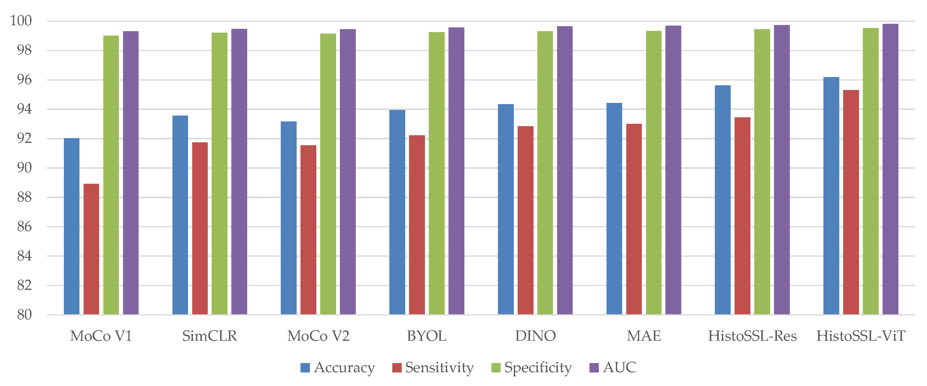
We performed experiments using modern self-supervised learning frameworks [2,3,4,5,6,25] on the NCTCRC and CAMELYON16 datasets. Experiments were conducted using the same pre-training dataset and evaluation protocols to ensure fairness. For MoCo V1 [2], MoCo V2 [6], SimCLR [3], and BYOL [4], we used ResNet-50 backbones, which was their out-of-the-box configuration. For DINO [5] and MAE [25], which are designed for vision transformers, we used the ViT-T/16 backbone. Our framework is backbone-agnostic. Therefore, the results of our proposed framework, HistoSSL, with both ResNet-50 and ViT-T/16 backbones are listed in

Table 5. Comparing our proposed method with the state-of-the-art frameworks on colorectal tissue phenotyping using the NCTCRC dataset.

Method	Year	Backbone	k-NN Accuracy (%)	Linear Probing Accuracy (%)
MoCo V1 [2]	2020	ResNet-50	87.67	92.02
SimCLR [3]	2020	ResNet-50	89.11	93.57
MoCo V2 [6]	2020	ResNet-50	90.18	93.15
BYOL [4]	2020	ResNet-50	90.74	93.93
DINO [5]	2021	ViT-T/16	93.23	94.34
MAE [25]	2022	ViT-T/16	92.60	94.42
HistoSSL-Res	Ours	ResNet-50	91.41	95.62
HistoSSL-ViT	Ours	ViT-T/16	94.09	96.18

and

Table 6. Comparing our proposed method with the state-of-the-art frameworks on breast cancer metastasis recognition using the CAMELYON16 dataset.

Method	Year	Backbone	k-NN Accuracy (%)	Linear Probing Accuracy (%)
MoCo V1 [2]	2020	ResNet-50	65.05	74.91
SimCLR [3]	2020	ResNet-50	71.12	76.97
MoCo V2 [6]	2020	ResNet-50	75.52	83.82
BYOL [4]	2020	ResNet-50	76.36	83.45
DINO [5]	2021	ViT-T/16	76.25	82.94
MAE [25]	2022	ViT-T/16	78.42	84.12
HistoSSL-Res	Ours	ResNet-50	78.21	83.60
HistoSSL-ViT	Ours	ViT-T/16	78.65	84.01

. The best results are highlighted in bold font. We also report the sensitivity, specificity, and AUC metrics of the linear classifier in Figure 4 and Figure 5. For the NCTCRC dataset, we used One-vs-Rest to evaluate the average sensitivity, specificity, and AUC for the nine classes.

As demonstrated in Table 5 and Figure 4, our proposed HistoSSL achieves state-of-the-art performance compared with mainstream contrastive learning counterparts using the same backbone and the same evaluation protocols, which proves its effectiveness. Specifically, by using ViT-T/16 as the backbone, the k-NN accuracy of HistoSSL is 94.09%; the accuracy, sensitivity, specificity, and AUC of the linear probing are 96.18%, 95.31%, 99.53%, and 99.82% respectively. The evaluations on the CAMELYON16 dataset are illustrated in Table 6 and Figure 5, where it is shown that HistoSSL also achieved the best k-NN accuracy (78.65%). During the linear evaluation, MAE [25] outperforms HistoSSL by 0.11% in accuracy and 0.17% in AUC.

5.2. Comparison with the Recent Studies

The above experiment aimed at a fair comparison of contrastive learning frameworks alone by using the same backbone and the same evaluation protocol. However, for the NCTCRC dataset, there are recent studies [8,9,34,37,38] introducing improvements from various aspects: introducing new backbones, exploiting large-scale pre-training sets, combining multiple self-supervised learning tasks, and using fine-tuning instead of linear probing to benefit from more trainable parameters. We present a comparison of these works. The results are listed in

Table 7. Comparing our proposed method with recent self-supervised learning studies on the NCTCRC dataset. The results are directly quoted from the corresponding literature.

Method	Year	BackBone	Accuracy (%)	Evaluation Protocol
CS-CO [34]	2021	ResNet-18	91.90	linear probing
SSLP [8]	2021	ResNet-18	95.20	linear probing
TransPath [9]	2021	CNN Transformer Hybrid	94.05	linear probing
TransPath [9]	2021	CNN Transformer Hybrid	95.85	fine-tuning
GC-MAE [37]	2022	ViT-B/16	89.22	fine-tuning
SD-MAE [38]	2022	ViT-S/16	95.04	fine-tuning
HistoSSL-Res	Ours	ResNet-50	95.62	linear probing
HistoSSL-ViT	Ours	ViT-T/16	96.18	linear probing

. The best result is highlighted with bold font.

From row 3 and row 4 in Table 7, we can observe that better results can be obtained in fine-tuning rather than linear probing for the same pre-trained backbone. This is because the backbone is frozen during linear probing. Thus, the model only has one trainable linear layer. While fine-tuning does not freeze the pre-trained backbone, the model benefits from more trainable parameters. However, fine-tuning requires more training effort on the downstream tasks and makes it difficult to solely evaluate the effectiveness of self-supervised pre-training. In our experiments, a tiny HistoSSL pre-trained model (ViT-T/16) can achieve state-of-the-art performance without the need for fine-tuning, which proves that HistoSSL can extract more robust representations for histopathology images.

To further evaluate the effectiveness of pre-training, linear probing, and fine-tuning, we report the results of the ResNet-50 model with the following settings: (a). supervised training from scratch, (b). linear probing on an ImageNet-pre-trained backbone, (c). linear probing on a HistoSSL-pre-trained backbone, (d). fine-tuning on an ImageNet-pre-trained backbone, (e). fine-tuning on a HistoSSL-pre-trained backbone. The results are listed in

Table 8. Results of the ResNet-50 model under different settings: a. supervised training from scratch, b. linear probing on an ImageNet-pre-trained backbone, c. linear probing on HistoSSL pre-trained backbone, d. fine-tuning on an ImageNet-pre-trained backbone, e. fine-tuning on HistoSSL pre-trained backbone.

Experiments	Accuracy (%)	Sensitivity (%)	Specificity (%)	AUC (%)
Supervised training (baseline)	91.65	88.40	98.96	99.29
Linear probing (ImageNet)	91.88	89.35	98.98	99.42
Linear probing (HistoSSL)	95.62	93.44	99.45	99.74
Fine-tuning (ImageNet)	95.55	94.72	99.45	99.66
Fine-tuning (HistoSSL)	96.55	95.25	99.58	99.76

.

In Table 8, we can observe that the accuracy of HistoSSL gets a $1\%$ boost by employing fine-tuning; it outperforms the supervised training baseline by $4.9\%$. HistoSSL pre-training also outperforms supervised ImageNet pre-training in both linear probing and fine-tuning.

5.3. Ablation Study

Generating positive views plays a decisive role in contrastive learning. Noisy views impair the model’s representation ability, whereas high-quality views can induce better representations [11]. Our proposed framework, HistoSSL, leverages random augmentations, cell-level patch extraction, and stain decomposition to generate positive samples from histopathology images. We performed ablated experiments with HistoSSL to verify the effectiveness of each method. The experiments were performed on the NCTCRC dataset. We used ViT-T/16 as the backbone. Results are listed in

Table 9. Ablation experiments of HistoSSL. We report the accuracies of both k-NN and linear probing under combinations of global-level, cell-level, and stain-level feature correspondence. The backbone was ViT-T/16.

Global	Cell	Stain	k-NN Accuracy (%)	Linear Probing Accuracy (%)
✓			91.27	93.31
✓	✓		93.36	95.02
✓	✓	✓	94.09	96.18

.

Global-level feature correspondence serves as a fundamental part of contrastive learning frameworks [2,3,4,5,6]. HistoSSL can achieve accuracies of 91.27% and 93.31% in k-NN and linear probing with only global-level feature correspondence.

Contrastive learning is prone to learn trivial low-level image statistics rather than holistic semantics if the low-level statistics are enough to contrast the positive from the negative. Most natural images have a few salient objects occupying a large portion of the area. Therefore, random crop-based augmentation can perturb the semantic information and force the model to learn high-level semantics to correctly distinguish the positive instances [2]. However, histopathology images are arrangements of relatively small and repeating cells, thereby having lower information density than natural images [25]. Randomly augmented views of histopathology images have a higher chance of sharing similar image statistics [11] and thus are less challenging. By leveraging cell-level patch extraction to incorporate cell-level views as positive samples, HistoSSL can have a performance gain of $1\%$ in k-NN and $1.7\%$ in linear probing.

Moreover, color deconvolution can decompose histopathology images into separated hematoxylin, eosin, and diaminobenzidine stains representing basophilic, acidophilic, and IHC-specific structures. Unlike cropping pixels spatially, stain decomposition splits the input image into different semantic entities. This simple yet effective method can generate meaningful and challenging positive samples that encourage the model to understand the image holistically. As demonstrated in Table 9, we observed a $1.1\%$ performance gain in linear probing and $0.7\%$ improvement in k-NN evaluation.

5.4. Comparison of Different Backbones

We performed experiments on various backbones, including classic CNNs: ResNets [41] and ResNeXT-50 [45]; a modern CNN: ConvNeXT-Small [46]; and vision transformers [42]. The results are listed in

Table 10. Comparison of different backbones. We report accuracy under k-NN and linear probing. The inference speed was tested on one NVIDIA Titan V GPU with mixed precision enabled.

Backbone	k-NN Accuracy (%)	Linear Probing Accuracy (%)	Speed (im/s)
ResNet-18 [41]	91.97	95.15	3399
ResNet-50 [41]	91.41	95.62	1820
ResNet-152 [41]	93.16	95.29	754
ResNeXt-50 [45]	92.45	94.44	1145
ConvNeXt-Small [46]	91.62	95.37	405
ViT-T/16 [42]	94.09	96.18	3002
ViT-S/16 [42]	94.50	95.87	1515
ViT-B/16 [42]	94.12	95.38	591
ViT-T/8 [42]	91.98	94.26	442

.

Transformers were first used in the natural language processing domain, in which self-supervised learning has been widely used. From Table 10, we can observe that a vision transformer [42] with patch size 16 demonstrated significant advantages over convolutional neural networks as the backbone in self-supervised learning. In our experiments, a ViT-T/16 model outperformed CNNs in both k-NN and linear probing. At the same time, ViT-T/16 has a comparable inference speed to ResNet-18, which is the fastest among the CNNs used in the experiments. We did not observe significant improvements in ResNeXt or ConvNeXt over standard ResNets. Meanwhile, their grouped convolution [45] and large kernel sizes [46] reduced the inference speed on GPUs.

One paper [5] showed that reducing the patch size from 16 to 8 can trade speed for performance. However, in our experiment, this approach impairs the accuracy in both k-NN and linear probing experiments. Moreover, halving the patch size will result in $4\times$ number of tokens, and the cost of computing self-attention scales quadratically with the number of tokens. Therefore, the inference speed of ViT-T/8 is significantly lower compared to that of ViT-T/16.

5.5. Comparison of Hyper-Parameters

5.5.1. Value of k in k-Nearest Neighbors

As introduced in Section 4.2.2, the k-NN classifier has only one hyper-parameter, k, which was set to 20 empirically. In this experiment, we used the ViT-S/16 backbone and performed a linear search for the proper value of k by 10-fold cross-validation. As illustrated in Figure 6, for a small value of k, the model is sensitive to outliers. Therefore, the accuracy is unstable. The model turned stable after $k>15$. To be consistent with the related works [5,6], and for brevity, we also set $k=20$.

5.5.2. Dimensions of the Model Output

As discussed in Section 3.1, the teacher and student models generated a K-dimensional probability distribution for each input image. We conducted experiments evaluating different values of K using the ViT-S/16 backbone on the NCTCRC dataset and reported k-NN accuracy. As illustrated in

Table 11. Comparison of different dimension size (K) using the ViT-S/16 backbone.

K	1024	2048	4096	10,240	20,480	40,960
Accuracy (%)	91.17	93.19	94.50	94.17	93.94	93.70

, we selected $K=4096$ in our experiments.

5.6. Discussion

In this study, we proposed HistoSSL to learn representations from unlabeled histopathology images. We evaluated HistoSSL on two tasks: colorectal tissue phenotyping on the NCTCRC dataset [15] and breast cancer metastasis recognition on the CAMELYON16 dataset [16]. HistoSSL achieved state-of-the-art performance with both k-NN and linear evaluation on the NCTCRC dataset (Table 5 and Table 7 and Figure 4). On the CAMELYON16 dataset, HistoSSL also achieved state-of-the-art performance in k-NN evaluation (Table 6 and Figure 5). Recently, MAE rejuvenated generative self-supervised learning by leveraging the power of multi-head self-attention and outperformed HistoSSL slightly in accuracy by $0.11\%$. We will investigate the way to incorporate histopathology domain knowledge into the generative model in the future.

We conducted experiments comparing HistoSSL pre-training with ImageNet pre-training and supervised learning from scratch (Table 8). We found that fine-tuning provides a $1\%$ performance gain over linear probing for the HistoSSL-pre-trained backbone. For the ImageNet-pre-trained backbone, the performance gain was $3.67\%$. This is because ImageNet is a dataset of natural images. Therefore, the pre-trained backbone lacks the domain knowledge of histopathology images and needs to be further tuned when transferring to the histopathology domain. Furthermore, we observe that supervised training from scratch cannot reach the same level of performance compared with HistoSSL pre-training. In fact, we observed that the model has a tendency of overfitting during supervised training. We hypothesize the reason is that the size of the NCRCRC dataset is not large enough. Since HistoSSL forms the training objective on the fly, the model is less prone to overfitting when pre-training on small datasets.

A series of backbone models, including both ConvNets and vision transformers, were tested in this study (Table 10). An interesting finding is that larger models do not necessarily lead to more significant performance gains, which can be seen for both the ResNet family [41] and the ViT family [42]. This does not fit the usual intuition about using larger models for self-supervised pre-training. We hypothesize the reason is that the pre-training dataset used in this experiment is not large enough (see Section 4.1). Therefore, the potential of large models is not fully leveraged. Due to the limitation of the computing resources we have available, we plan to investigate large models on bigger datasets in our future work.

6. Conclusions

In this study, we proposed a self-supervised representation learning framework, HistoSSL, for unlabeled histopathology images. Unlike conventional self-supervised learning approaches, HistoSSL leverages the cell-level and stain-level feature correspondence in histopathology images to learn more robust representations. HistoSSL achieved higher accuracies than the state-of-the-art self-supervised learning approaches on the NCTCRC and CAMELYON16 datasets. In the future, we will investigate the effectiveness of large-scale pre-training data with large models. Moreover, we aim to explore how to incorporate histopathology domain knowledge into the generative masked image models.

References

- Wang, D.; Khosla, A.; Gargeya, R.; Irshad, H.; Beck, A.H. Deep learning for identifying metastatic breast cancer. arXiv 2016, arXiv:1606.05718. [Google Scholar]
- He, K.; Fan, H.; Wu, Y.; Xie, S.; Girshick, R. Momentum contrast for unsupervised visual representation learning. In Proceedings of the IEEE/CVF Conference on Computer Vision and Pattern Recognition, Seattle, WA, USA, 13–19 June 2020; pp. 9729–9738. [Google Scholar]
- Chen, T.; Kornblith, S.; Norouzi, M.; Hinton, G. A simple framework for contrastive learning of visual representations. In Proceedings of the International Conference on Machine Learning, Online, 12–18 July 2020; PMLR: Cambridge, MA, USA, 2020; pp. 1597–1607. [Google Scholar]
- Grill, J.B.; Strub, F.; Altché, F.; Tallec, C.; Richemond, P.; Buchatskaya, E.; Doersch, C.; Avila Pires, B.; Guo, Z.; Gheshlaghi Azar, M.; et al. Bootstrap your own latent-a new approach to self-supervised learning. Adv. Neural Inf. Process. Syst. 2020, 33, 21271–21284. [Google Scholar]
- Caron, M.; Touvron, H.; Misra, I.; Jégou, H.; Mairal, J.; Bojanowski, P.; Joulin, A. Emerging properties in self-supervised vision transformers. In Proceedings of the IEEE/CVF International Conference on Computer Vision, Montreal, BC, Canada, 11–17 October 2021; pp. 9650–9660. [Google Scholar]
- Chen, X.; Fan, H.; Girshick, R.; He, K. Improved baselines with momentum contrastive learning. arXiv 2020, arXiv:2003.04297. [Google Scholar]
- Wang, X.; Yang, S.; Zhang, J.; Wang, M.; Zhang, J.; Yang, W.; Huang, J.; Han, X. Transformer-based unsupervised contrastive learning for histopathological image classification. Med. Image Anal. 2022, 81, 102559. [Google Scholar] [CrossRef] [PubMed]
- Li, J.; Lin, T.; Xu, Y. SSLP: Spatial Guided Self-supervised Learning on Pathological Images. In Proceedings of the International Conference on Medical Image Computing and Computer-Assisted Intervention, Strasbourg, France, 27 September–1 October 2021; Springer: Berlin/Heidelberg, Germany, 2021; pp. 3–12. [Google Scholar]
- Wang, X.; Yang, S.; Zhang, J.; Wang, M.; Zhang, J.; Huang, J.; Yang, W.; Han, X. Transpath: Transformer-based self-supervised learning for histopathological image classification. In Proceedings of the International Conference on Medical Image Computing and Computer-Assisted Intervention, Strasbourg, France, 27 September–1 October 2021; Springer: Berlin/Heidelberg, Germany, 2021; pp. 186–195. [Google Scholar]
- Chen, R.J.; Chen, C.; Li, Y.; Chen, T.Y.; Trister, A.D.; Krishnan, R.G.; Mahmood, F. Scaling Vision Transformers to Gigapixel Images via Hierarchical Self-Supervised Learning. In Proceedings of the IEEE/CVF Conference on Computer Vision and Pattern Recognition, Vancouver, BC, Canada, 81–23 June 2022; pp. 16144–16155. [Google Scholar]
- Ciga, O.; Xu, T.; Martel, A.L. Self supervised contrastive learning for digital histopathology. Mach. Learn. Appl. 2022, 7, 100198. [Google Scholar] [CrossRef]
- Titford, M. Progress in the development of microscopical techniques for diagnostic pathology. J. Histotechnol. 2009, 32, 9–19. [Google Scholar] [CrossRef]
- Chan, J.K. The wonderful colors of the hematoxylin—Eosin stain in diagnostic surgical pathology. Int. J. Surg. Pathol. 2014, 22, 12–32. [Google Scholar] [CrossRef]
- Ruifrok, A.C.; Johnston, D.A. Quantification of histochemical staining by color deconvolution. Anal. Quant. Cytol. Histol. 2001, 23, 291–299. [Google Scholar]
- Kather, J.N.; Halama, N.; Marx, A. 100,000 Histological Images of Human Colorectal Cancer and Healthy Tissue. 2018. Available online: https://zenodo.org/record/1214456#.Y6lhPvdBxPY (accessed on 11 November 2022).
- Litjens, G.; Bandi, P.; Ehteshami Bejnordi, B.; Geessink, O.; Balkenhol, M.; Bult, P.; Halilovic, A.; Hermsen, M.; van de Loo, R.; Vogels, R.; et al. 1399 H&E-stained sentinel lymph node sections of breast cancer patients: The CAMELYON dataset. GigaScience 2018, 7, giy065. [Google Scholar]
- Bejnordi, B.E.; Veta, M.; Van Diest, P.J.; Van Ginneken, B.; Karssemeijer, N.; Litjens, G.; Van Der Laak, J.A.; Hermsen, M.; Manson, Q.F.; Balkenhol, M.; et al. Diagnostic assessment of deep learning algorithms for detection of lymph node metastases in women with breast cancer. JAMA 2017, 318, 2199–2210. [Google Scholar] [CrossRef] [Green Version]
- Ye, M.; Zhang, X.; Yuen, P.C.; Chang, S.F. Unsupervised embedding learning via invariant and spreading instance feature. In Proceedings of the IEEE/CVF Conference on Computer Vision and Pattern Recognition, Long Beach, CA, USA, 16–17 June 2019; pp. 6210–6219. [Google Scholar]
- Qu, L.; Liu, S.; Liu, X.; Wang, M.; Song, Z. Towards label-efficient automatic diagnosis and analysis: A comprehensive survey of advanced deep learning-based weakly-supervised, semi-supervised and self-supervised techniques in histopathological image analysis. Phys. Med. Biol. 2022, 67, 20TR01. [Google Scholar] [CrossRef] [PubMed]
- Hinton, G.E.; Zemel, R. Autoencoders, minimum description length and Helmholtz free energy. In Proceedings of the Advances in Neural Information Processing Systems 30 (NIPS 1993), Denver, CO, USA, 29 November–2 December 1993; Volume 6. [Google Scholar]
- Pathak, D.; Krahenbuhl, P.; Donahue, J.; Darrell, T.; Efros, A.A. Context encoders: Feature learning by inpainting. In Proceedings of the IEEE Conference on Computer Vision and Pattern Recognition, Las Vegas, NV, USA, 27–30 June 2016; pp. 2536–2544. [Google Scholar]
- Zhang, R.; Isola, P.; Efros, A.A. Colorful image colorization. In Proceedings of the European Conference on Computer Vision, Amsterdam, The Netherlands, 11–14 October 2016; Springer: Berlin/Heidelberg, Germany, 2016; pp. 649–666. [Google Scholar]
- Devlin, J.; Chang, M.W.; Lee, K.; Toutanova, K. Bert: Pre-training of deep bidirectional transformers for language understanding. arXiv 2018, arXiv:1810.04805. [Google Scholar]
- Chen, M.; Radford, A.; Child, R.; Wu, J.; Jun, H.; Luan, D.; Sutskever, I. Generative pretraining from pixels. In Proceedings of the International Conference on Machine Learning, Online, 13–18 July 2020; PMLR: Cambridge, MA, USA, 2020; pp. 1691–1703. [Google Scholar]
- He, K.; Chen, X.; Xie, S.; Li, Y.; Dollár, P.; Girshick, R. Masked autoencoders are scalable vision learners. In Proceedings of the IEEE/CVF Conference on Computer Vision and Pattern Recognition, Vancouver, BC, Canada, 18–23 June 2022; pp. 16000–16009. [Google Scholar]
- Noroozi, M.; Favaro, P. Unsupervised learning of visual representations by solving jigsaw puzzles. In Proceedings of the European Conference on Computer Vision, Amsterdam, The Netherlands, 11–14 October 2016; Springer: Berlin/Heidelberg, Germany, 2016; pp. 69–84. [Google Scholar]
- Gidaris, S.; Singh, P.; Komodakis, N. Unsupervised representation learning by predicting image rotations. arXiv 2018, arXiv:1803.07728. [Google Scholar]
- Oord, A.v.d.; Li, Y.; Vinyals, O. Representation learning with contrastive predictive coding. arXiv 2018, arXiv:1807.03748. [Google Scholar]
- Chen, X.; He, K. Exploring simple siamese representation learning. In Proceedings of the IEEE/CVF Conference on Computer Vision and Pattern Recognition, Nashville, TN, USA, 20–25 June 2021; pp. 15750–15758. [Google Scholar]
- Chen, X.; Xie, S.; He, K. An empirical study of training self-supervised vision transformers. In Proceedings of the IEEE/CVF International Conference on Computer Vision, Online, 11–17 October 2021; pp. 9640–9649. [Google Scholar]
- Wu, Z.; Xiong, Y.; Yu, S.X.; Lin, D. Unsupervised feature learning via non-parametric instance discrimination. In Proceedings of the IEEE Conference on Computer Vision and Pattern Recognition, Salt Lake City, UT, USA, 18–22 June 2018; pp. 3733–3742. [Google Scholar]
- Tarvainen, A.; Valpola, H. Mean teachers are better role models: Weight-averaged consistency targets improve semi-supervised deep learning results. In Proceedings of the Advances in Neural Information Processing Systems 30 (NIPS 2017), Long Beach, CA, USA, 4–9 December 2017; Volume 30. [Google Scholar]
- Liu, Y.; Gadepalli, K.; Norouzi, M.; Dahl, G.E.; Kohlberger, T.; Boyko, A.; Venugopalan, S.; Timofeev, A.; Nelson, P.Q.; Corrado, G.S.; et al. Detecting cancer metastases on gigapixel pathology images. arXiv 2017, arXiv:1703.02442. [Google Scholar]
- Yang, P.; Hong, Z.; Yin, X.; Zhu, C.; Jiang, R. Self-supervised visual representation learning for histopathological images. In Proceedings of the International Conference on Medical Image Computing and Computer-Assisted Intervention, Strasbourg, France, 27 September–1 October 2021; Springer: Berlin/Heidelberg, Germany, 2021; pp. 47–57. [Google Scholar]
- Lin, Y.; Qu, Z.; Chen, H.; Gao, Z.; Li, Y.; Xia, L.; Ma, K.; Zheng, Y.; Cheng, K.T. Label Propagation for Annotation-Efficient Nuclei Segmentation from Pathology Images. arXiv 2022, arXiv:2202.08195. [Google Scholar]
- Koohbanani, N.A.; Unnikrishnan, B.; Khurram, S.A.; Krishnaswamy, P.; Rajpoot, N. Self-path: Self-supervision for classification of pathology images with limited annotations. IEEE Trans. Med. Imaging 2021, 40, 2845–2856. [Google Scholar] [CrossRef]
- Quan, H.; Li, X.; Chen, W.; Zou, M.; Yang, R.; Zheng, T.; Qi, R.; Gao, X.; Cui, X. Global Contrast Masked Autoencoders Are Powerful Pathological Representation Learners. arXiv 2022, arXiv:2205.09048. [Google Scholar]
- Luo, Y.; Chen, Z.; Gao, X. Self-distillation augmented masked autoencoders for histopathological image classification. arXiv 2022, arXiv:2203.16983. [Google Scholar]
- Sahasrabudhe, M.; Christodoulidis, S.; Salgado, R.; Michiels, S.; Loi, S.; André, F.; Paragios, N.; Vakalopoulou, M. Self-supervised nuclei segmentation in histopathological images using attention. In Proceedings of the International Conference on Medical Image Computing and Computer-Assisted Intervention, Lima, Peru, 4–8 October 2020; Springer: Berlin/Heidelberg, Germany, 2020; pp. 393–402. [Google Scholar]
- Jahne, B. Practical Handbook on Image Processing for Scientific and Technical Applications; CRC Press: Boca Raton, FL, USA, 2004. [Google Scholar]
- He, K.; Zhang, X.; Ren, S.; Sun, J. Deep residual learning for image recognition. In Proceedings of the IEEE Conference on Computer Vision and Pattern Recognition, Las Vegas, NV, USA, 27–30 June 2016; pp. 770–778. [Google Scholar]
- Dosovitskiy, A.; Beyer, L.; Kolesnikov, A.; Weissenborn, D.; Zhai, X.; Unterthiner, T.; Dehghani, M.; Minderer, M.; Heigold, G.; Gelly, S.; et al. An image is worth 16 ×16 words: Transformers for image recognition at scale. arXiv 2020, arXiv:2010.11929. [Google Scholar]
- Goode, A.; Gilbert, B.; Harkes, J.; Jukic, D.; Satyanarayanan, M. OpenSlide: A vendor-neutral software foundation for digital pathology. J. Pathol. Inform. 2013, 4, 27. [Google Scholar] [CrossRef] [PubMed]
- Paszke, A.; Gross, S.; Massa, F.; Lerer, A.; Bradbury, J.; Chanan, G.; Killeen, T.; Lin, Z.; Gimelshein, N.; Antiga, L.; et al. Pytorch: An imperative style, high-performance deep learning library. In Proceedings of the Advances in Neural Information Processing Systems 32 (NeurIPS 2019), Vancouver, BC, Canada, 8–14 December 2019; Volume 32. [Google Scholar]
- Xie, S.; Girshick, R.; Dollár, P.; Tu, Z.; He, K. Aggregated residual transformations for deep neural networks. In Proceedings of the IEEE Conference on Computer Vision and Pattern Recognition, Honolulu, HI, USA, 21–26 July 2017; pp. 1492–1500. [Google Scholar]
- Liu, Z.; Mao, H.; Wu, C.Y.; Feichtenhofer, C.; Darrell, T.; Xie, S. A convnet for the 2020s. In Proceedings of the IEEE/CVF Conference on Computer Vision and Pattern Recognition, Vancouver, BC, Canada, 18–23 June 2022; pp. 11976–11986. [Google Scholar]
Figure 1.
Illustration of our proposed framework, HistoSSL. HistoSSL learns representations from the feature correspondence by performing knowledge distillation. The student model is trained by aligning the student’s output distribution with the teacher’s distribution. Knowledge distillation is performed at three levels: global-, cell-, and stain-level. Global-level views are generated via random augmentations, cell-level views are generated by extracting cell-level patches, and stain-level views are generated from stain decomposition. The parameters of the teacher network are an exponential momentum average (EMA) of the student.
Figure 2.
Overview of the network model. The backbone takes an image as input and outputs a F-dim vector as its representation. The head projects the representation vector into a K-dim distribution for knowledge distillation.
Figure 3.
Vision transformers split input images into non-overlapping patches and use linear projection to convert these patches into a 1-dim token sequence. To handle variable input sizes, we interpolate the positional encoding to match the number of tokens. The flattened positional encodings are then added to the token sequence.
Figure 4.
Sensitivity, specificity, and AUC results (%) on the NCTCRC dataset.
Figure 5.
Sensitivity, specificity, and AUC results (%) on the CAMELYON16 dataset.
Figure 6.
Comparison of different k in k-NN classifiers.