Application of the ADMM Algorithm for a High-Dimensional Partially Linear Model

Abstract

This paper focuses on a high-dimensional semi-parametric regression model in which a partially linear model is used for the parametric part and the B-spline basis function approach is used to estimate the unknown function for the non-parametric part. Within the framework of this model, the constrained least squares estimation is investigated, and the alternating-direction multiplier method (ADMM) is used to solve the model. The convergence is proved under certain conditions. Finally, numerical simulations are performed and applied to workers’ wage data from CPS85. The results show that the ADMM algorithm is very effective in solving high-dimensional partially linear models.

1. Introduction

With the rapid development of modern technology, many fields have generated high-dimensional data, such as in biological information, biomedicine, meteorology, geography, econometrics, machine learning, etc. The term “high-dimensional” refers to the fact that the number of variables in data is much larger than the number of samples. In practical situations, the actual structure of a model is often unknown. If only parametric or non-parametric regression models are used for statistical inference, the results will produce large biases and erroneous conclusions. Therefore, semi-parametric regression models came into being in the 1980s, and Engle first proposed semi-parametric regression models, which contain both parametric and non-parametric components. These are more widely used than parametric or non-parametric models. A semi-parametric regression model is a statistical model in which:

$$Y=g(X,\beta )+m\left(U\right)+\epsilon ,$$

(1)

where Y is a real-valued response variable, $\beta \in R^p$ is a p-dimensional unknown parameter vector, X is a d-dimensional covariate, and $g(·,·)$ is a known and measurable function. $U\in [0,1]$ is a random variable, $m(·)$ is a smooth unknown function defined on $[0,1]$, and $\epsilon$ is a random error.

This paper focuses on high-dimensional semi-parametric regression models in which a partially linear model is used for the parametric part. A partially linear model was proposed by Engle [1] in 1986 when he studied weather and electricity problems. The response variables of the model had linear relationships with some covariates and nonparametric relationships with other covariates, so the partially linear model combined the advantages of the interpretability of linear models with the flexibility of non-parametric models. Partial linear models have been studied by many scholars, such as Heckman (1986) [2], Xu (2019) [3], Chen (2020) [4], Auerbach (2022) [5], etc., and they have achieved many results. Among them, Heckman (1986) [2] proposed a partially linear model with a smooth spline and obtained the consistency and asymptotic normality of the parameter estimation based on Bayesian estimation. Härdle (2000) [6] reviewed a series of studies on partially linear models. In the non-parametric part, the B-spline basis function method was used to estimate the unknown function. The B-spline basis function method is a global smoothing method, and its calculation accuracy and efficiency are relatively high. Numerous scholars have studied and achieved many results for high-dimensional data, such as those of Lasso [7,8,9], SCAD (smoothly clipped absolute deviation) [10,11,12], and MCP (minimax concave penalty) [13,14], and many scholars have also performed much research on high-dimensional partially linear models. Xie (2009) [10] studied SCAD-penalized regression in high-dimensional partially linear models by using polynomial regression splines to estimate the non-parametric part; Ni (2009) [15] proposed a double-penalty partially linear variable selection method that used smooth splines to estimate the non-parametric part. In the case of parameter dispersion, Chen (2012) [16] studied the variable selection problem for the contour-adaptive Elastic-Net for a partially linear model with high-dimensional covariates; Wang (2017) [17] studied constrained-contour least squares estimation based on contour Lagrange multiplier test statistics with linear constraints and gave the convergence speed and asymptotic normality of the least squares estimation.

Wang considered the following partially linear regression model (PLM):

$$Y=X^{\mathrm{T}}\beta +B{}^{\mathrm{T}}\gamma +\epsilon ,$$

(2)

where Y is a univariate response variable, $X={(X_1,\dots ,X_p)}^{\mathrm{T}}\in R^p$, and $\mathrm{Z}\in \mathrm{R}$ are explanatory variables. We denote $Y={(Y_1,\dots ,Y_n)}^{\mathrm{T}}$; $X={(X_1,\dots ,X_n)}^{\mathrm{T}}$; $\beta ={({\beta }_1,\dots ,{\beta }_p)}^{\mathrm{T}}$ is an unknown p-dimensional parameter vector; $\epsilon ={({\epsilon }_1,\dots ,{\epsilon }_n)}^{\mathrm{T}}$. $B=B\left(Z\right)={(B_1\left(Z\right),\dots ,B_{m_n}\left(Z\right))}^{\mathrm{T}}$ is a set of B-spline basis functions of order r, and $\gamma ={({\gamma }_1,\dots ,{\gamma }_{m_n})}^{\mathrm{T}}$ is a spline coefficient vector.

Let $(Y_1;X_1^{\mathrm{T}};Z_1)\dots (Y_n;X_n^{\mathrm{T}};Z_n)$ be an independent identically distributed sample of the size of the model. We denote $X_i={(X_{i1},\dots ,X_{ip})}^{\mathrm{T}}$; model (2) can be approximated by:

$$Y_i={X_i}^{\mathrm{T}}\beta +B{\left(Z_i\right)}^{\mathrm{T}}\gamma +{\epsilon }_i.$$

(3)

From Equation (3), we can obtain $\epsilon =Y-X\beta -B\gamma$. By using the least squares method to estimate the parameters $\beta$ and $\gamma$, minimizing the error is equivalent to:

$$\underset{\beta ,\gamma }{min}\frac{1}{2}{∥Y-X\beta -B\gamma ∥}^2.$$

(4)

In practice, the parameter estimates can also be improved by adding prior information about the regression parameters. The constraint condition is the profile Lagrange multiplier test statistic proposed by Wei and Wu (2008) [18]:

$$R\beta =d,$$

(5)

where R is a given $k\times p$ matrix whose rank is k, and d is a known k-dimensional vector.

The study in this paper is equivalent to the solution of the following optimization problem:

$$\begin{array}{c}\underset{\beta ,\gamma }{\min }\frac{1}{2}{∥Y-X\beta -B\gamma ∥}^2,\hfill \\ s.t.R\beta =d.\hfill \end{array}$$

(6)

Wang (2017) [17] studied restricted profile least squares estimation, and a Lagrangian function was constructed based on linear constraints. The parameter estimation was performed by using the Lagrange multiplier method. The results showed that the algorithm was efficient when parameter information was available.

Our study considers the optimization problem in (6) by constructing an augmented Lagrangian function with linear constraints and using the alternating-direction method of multipliers (ADMM) to solve the model. The Lagrange multiplier update is a kind of ascending iteration, and its convergence can only be moderately accelerated. Therefore, the Lagrange multiplier method is more time-consuming. The augmented Lagrange multiplier method is a method that combines the Lagrange multiplier method and a penalty function method in one piece, so it is a simple and effective method. Hestenes [19] and Powell [20] first proposed the augmented Lagrangian function and multiplier method for constrained optimization in the late 1960s. The ADMM [21] is a classical algorithm for solving nonlinear problems that was proposed by Glowinski and Marroco in the 1970s. The ADMM is very suitable for convex optimization [22]. This algorithm has a large number of applications in different fields, such as regularized estimation [23], image processing [24], machine learning [25], optimal control [26], and resource allocation for wireless networks [27]. When the scale of a problem is relatively large, a distributed algorithm is faster. Considering the characteristics of the optimization problem in (6), it can be solved in blocks. This is suitable for the algorithmic framework of the ADMM, so this paper will use the ADMM to solve the high-dimensional partially linear model.

2. Introduction to the ADMM Algorithm

In this part, we summarize some useful content for the following discussion.

Firstly, we briefly review the basic knowledge of the ADMM. Our motivation is to apply the ADMM to solve the model in this paper. Let us start from a general convex minimization problem with a separable objective function and linear constraints:

$$\begin{array}{l}\min f\left(x\right)+g\left(z\right),\\ s.t.Ax+Bz=c,\end{array}$$

(7)

where $x\in R^m$, $z\in R^n$, $A\in R^{p\times m}$, $B\in R^{p\times n}$, $c\in R^p$, $f:R^m\in R$, and $g:R^n\in R$. x and z are independent variables. The augmented Lagrangian function of the minimization problem is:

$$L_p(x,y,z)=f\left(x\right)+g\left(z\right)+y^{\mathrm{T}}(Ax+Bz-c)+\frac{p}{2}{∥Ax+Bz-c∥}_2^2,$$

(8)

where y is the Lagrange multiplier and $p>0$ is a penalty parameter. The minimization problem can be solved with the augmented Lagrange multiplier method. With a given $y^0$, the iterative scheme of the augmented Lagrangian function for the minimization problem is:

$$\left\{\begin{array}{l}(x^{k+1},z^{k+1}):=argmin\left\{L_p(x,y,z^k)\right\},\\ y^{k+1}:=y^k-p(A{x}^{k+1}+B{z}^{k+1}-c).\end{array}\right.$$

(9)

The iterative scheme is an application of the augmented Lagrangian function method for solving the above iterations, which require the simultaneous polarization of the variables x and z in each iteration. In addition, the ADMM algorithm decomposes the above iteration into two parts [28] and continuously minimizes the variables; it is expressed as follows:

$$\left\{\begin{array}{c}\begin{array}{c}{x}^{k+1}:=argmin\left\{L_p(x,y^k,z^k)\right\},\\ z^{k+1}:=argmin\left\{L_p(x^{k+1},y,z^k)\right\},\end{array}\\ y^{k+1}:=y^k-p(A{x}^{k+1}+B{z}^{k+1}-c).\end{array}\right.$$

(10)

The ADMM is widely used, and it is of interest that the subproblem generated by the ADMM must exist in the form of an analytical solution in each iteration.

3. Model and Algorithm

In this section, we will apply the ADMM algorithm to solve the minimization model in this paper and to derive the analytical solution form of each subproblem.

3.1. The High-Dimensional Partially Linear Model

For the optimization problem in (6), by using the augmented Lagrange multiplier method, the constrained programming problem is transformed into an unconstrained optimization problem, and the augmented Lagrangian function is:

$$min{L}_{\rho }(\beta ,\gamma ,\lambda )=\frac{1}{2}{∥Y-X\beta -B\gamma ∥}^2+〈\lambda ,R\beta -d〉+\frac{\rho }{2}{∥R\beta -d∥}^2.$$

(11)

Using the alternating-direction method of multipliers (ADMM), its n-step iteration starts from a given $({\beta }^n,{\lambda }^n)$ with:

$$\left\{\begin{array}{c}{\gamma }^{n+1}=arg\underset{\gamma }{min}{L}_{\rho }({\beta }^n,\gamma ,{\lambda }^n),\\ {\beta }^{n+1}=arg\underset{\beta }{min}{L}_{\rho }(\beta ,{\gamma }^{n+1},{\lambda }^n),\\ {\lambda }^{n+1}={\lambda }^n+\rho (R{\beta }^{n+1}-d).\end{array}\right.$$

(12)

We get the new iteration point at $({\gamma }^{n+1},{\beta }^{n+1},{\lambda }^{n+1})$.

3.2. Solution of the ADMM for High-Dimensional Partially Linear Models

After a simple calculation, the $\gamma$-subproblem in Equation (11) can be written as the following equation:

$${\gamma }^{n+1}=arg\underset{\gamma }{min}\{\frac{1}{2}{∥Y-X{\beta }^n-B\gamma ∥}^2\}.$$

(13)

According to the above method, one can find the partial derivative of $\gamma$ for any given $\beta$:

$$\frac{\partial L_{\rho }(\beta ,\gamma ,\lambda )}{\partial \gamma }=-B(Y-X{\beta }^n-B\gamma )=0.$$

(14)

The analytical solution of $\gamma$ can be obtained in the form of:

$${\gamma }^{n+1}={\left(B^{\mathrm{T}}B\right)}^{-1}{B}^{\mathrm{T}}(Y-X{\beta }^n).$$

(15)

For the analytical solution of $\beta$, the objective function can be solved by substituting $\gamma$ into Equation (11):

$${\beta }^{n+1}=arg\underset{\beta }{min}\{\frac{1}{2}{∥Y-X\beta -B{\gamma }^{n+1}∥}^2+〈{\lambda }^n,R\beta -d〉+\frac{\rho }{2}{∥R\beta -d∥}^2\},$$

(16)

with the following partial derivatives for $\beta$:

$$\frac{\partial L_{\rho }(\beta ,{\gamma }^{n+1},{\lambda }^n)}{\partial \beta }={(X{X}^{\mathrm{T}}+\rho R{R}^{\mathrm{T}})}^{-1}(X^{\mathrm{T}}(Y-B{\gamma }^{n+1})+R^{\mathrm{T}}(\rho d-{\lambda }^n))=0.$$

(17)

The solutions ${\gamma }^{n+1}$, ${\beta }^{n+1}$, and ${\lambda }^{n+1}$ are solved by calculating:

$$\left\{\begin{array}{c}{\gamma }^{n+1}={\left(B^{\mathrm{T}}B\right)}^{-1}{B}^{\mathrm{T}}(Y-X{\beta }^n),\\ {\beta }^{n+1}={(X{X}^{\mathrm{T}}+\rho R{R}^{\mathrm{T}})}^{-1}(X^{\mathrm{T}}(Y-B{\gamma }^{n+1})+R^{\mathrm{T}}(\rho d-{\lambda }^n)),\\ {\lambda }^{n+1}={\lambda }^n+\rho (R{\beta }^{n+1}-d).\end{array}\right.$$

(18)

3.3. Algorithmic Design of ADMM for Solving High-Dimensional Partially Linear Models

In summary, the iterative algorithm for solving high-dimensional partially linear models by using the ADMM can be described as follows.

Step 1. Input the variables X, Y, and B, and given the initial variables $({\beta }^0,{\gamma }^0,{\lambda }^0)$, select the penalty parameter where $\rho >0$;

Step 2. Input the iteration step $n=1,2,\dots ,N$;

Step 3. Update the parameters ${\gamma }^{n+1}$, ${\beta }^{n+1}$, and ${\lambda }^{n+1}$ with Equation (18);

Step 4. Iterate through the loop, returning to step 3 until the termination conditions are met, and the algorithm is terminated;

Step 5. Output $({\beta }^N,{\gamma }^N,{\lambda }^N)$ as the approximate solution $({\beta }^{*},{\gamma }^{*},{\lambda }^{*})$ of (6).

4. Convergence

In this section, we will use a variational inequality to prove the convergence of the algorithm. The Lagrange function of the model is given by:

$$L(\beta ,\gamma ,\lambda )=\frac{1}{2}{∥Y-X\beta -B\gamma ∥}^2+〈\lambda ,R\beta -d〉,$$

(19)

where $\lambda$ is the Lagrange multiplier.

The solution of Equation (11) is equivalent to finding $({\gamma }^{*},{\beta }^{*},{\lambda }^{*})\in S$ such that:

$$\left\{\begin{array}{c}{B}^{\mathrm{T}}X{\beta }^{*}+B^{\mathrm{T}}B{\gamma }^{*}-B^{\mathrm{T}}Y=0,\\ {(X{X}^{\mathrm{T}}+\rho R{R}^{\mathrm{T}})}^{-1}(X^{\mathrm{T}}(Y-B{\gamma }^{*})+R^{\mathrm{T}}(\rho d-{\lambda }^{*}))=0,\\ R^{\mathrm{T}}{\beta }^{*}-d=0.\end{array}\right.$$

(20)

Let $S^{*}$ satisfy Equation (19); then, we define ${\omega }^{*}=({\gamma }^{*},{\beta }^{*},{\lambda }^{*})\in S^{*}$. Equation (19) is equivalent to a variational problem. We find $({\gamma }^{*},{\beta }^{*},{\lambda }^{*})\in S^{*}$ such that the following variational inequality holds:

$$VI(S,F):(\omega -{\omega }^{*})F\left({\omega }^{*}\right)\ge 0,\forall \omega \in S.$$

(21)

Here,

$$\omega =\left(\begin{array}{c}\gamma \\ \beta \\ \lambda \end{array}\right),F\left(\omega \right)=\left(\begin{array}{c}{B}^{\mathrm{T}}X\beta +B^{\mathrm{T}}B\gamma -B^{\mathrm{T}}Y\\ {(X{X}^{\mathrm{T}}+\rho R{R}^{\mathrm{T}})}^{-1}(X^{\mathrm{T}}(Y-B\gamma )+R^{\mathrm{T}}(\rho d-\lambda ))\\ R^{\mathrm{T}}\beta -d.\end{array}\right)$$

(22)

We need to use the positive definite matrix G:

$$G=\left(\begin{array}{ccc}\mu I_p-{\widehat{X}}^{\mathrm{T}}\widehat{X}& 0& 0\\ 0& \rho I_p& 0\\ 0& 0& \frac{1}{\rho }{I}_p\end{array}\right),$$

(23)

where $\widehat{X}={(X^{\mathrm{T}},\sqrt{\rho }R)}^{\mathrm{T}}$. For the positive definite matrix G, the following conditions are satisfied: $\mu >\tau (X^{\mathrm{T}}X+\rho R^{\mathrm{T}}R)$ and $\mu (·)$ is the spectral radius of the matrix.

In order to establish the convergence of the algorithm, the $n+1$th iteration value of the algorithm is taken as a variational inequality problem. The following lemma can be obtained.

Lemma 1. 

Let $\left\{{\omega }^n\right\}$ denote the sequence generated by the algorithm; then, for any ${\omega }^{\prime }\in S$,

$$({\omega }^{\prime }-{\omega }^{n+1})(F\left({\omega }^{n+1}\right)+M({\beta }^n-{\beta }^{n+1})-G({\omega }^n-{\omega }^{n+1}))\ge 0,$$

where,

$$M=\left(\begin{array}{c}-\rho R^{\mathrm{T}}\\ \rho I_p\\ 0_p\end{array}\right).$$

Lemma 2. 

Let $\left\{{\omega }^n\right\}$ denote the sequence generated by the algorithm; then, for any ${\omega }^{*}\in S^{*}$,

$${({\omega }^n-{\omega }^{*})}^{\mathrm{T}}G({\omega }^n-{\omega }^{n+1})\ge {({\omega }^n-{\omega }^{n+1})}^{\mathrm{T}}G({\omega }^n-{\omega }^{n+1})-{({\lambda }^n-{\lambda }^{n+1})}^{\mathrm{T}}({\beta }^n-{\beta }^{n+1}).$$

Lemma 3. 

Let $\left\{{\omega }^n\right\}$ denote the sequence generated by the algorithm; then, for any ${\omega }^{*}\in S^{*}$,

$$\left|\right|{\omega }^{n+1}-{\omega }^{*}{\left|\right|}_G^2\le \left|\right|{\omega }^n-{\omega }^{*}{\left|\right|}_G^2-\left|\right|{\omega }^n-{\omega }^{n+1}{\left|\right|}_G^2$$

From Lemmas 1 and 2, it can be proved that the sequence $\left\{{\omega }^n\right\}$ generated by this algorithm shrinks to the solution set $S^{*}$. Lemma 3 shows that the sequence $\left\{{\omega }^n\right\}$ generated by the algorithm shrinks to the solution set S, and the following corollary can be obtained from Lemma 3.

Corollary 1. 

Let the sequence be generated by the algorithm; then, we get:

• $\underset{k\to \infty }{lim}{∥{\omega }^n-{\omega }^{n+1}∥}_G=0$;
• The sequence $\left\{{\omega }^n\right\}$ is bounded;
• For arbitrary ${\omega }^{*}\in S^{*}$, the sequence $\left\{{∥{\omega }^n-{\omega }^{*}∥}_G\right\}$ is non-increasing.

Theorem 1. 

Given any starting point $({\gamma }^0,{\beta }^0,{\lambda }^0)\in S$, for any $\rho \ge 0$, $\mu >\tau (X^{\mathrm{T}}X+\rho R^{\mathrm{T}}R)$, the sequence $\left\{{\omega }^n=({\gamma }^n,{\beta }^n,{\lambda }^n)\right\}$ is generated by the algorithm and converges to $\left\{{\omega }^{\infty }=({\gamma }^{\infty },{\beta }^{\infty },{\lambda }^{\infty })\right\}$, where $({\gamma }^{\infty },{\beta }^{\infty },{\lambda }^{\infty })$ is the solution of the model.

Proof. 

From Property 1 of Corollary 3, we can get:

$$\left\{\begin{array}{c}\underset{k\to \infty }{lim}\left|\right|{\gamma }^n-{\gamma }^{n+1}\left|\right|=0,\\ \underset{k\to \infty }{lim}\left|\right|{\beta }^n-{\beta }^{n+1}\left|\right|=0,\\ \underset{k\to \infty }{lim}\left|\right|{\lambda }^n-{\lambda }^{n+1}\left|\right|=0.\end{array}\right.$$

(24)

By Property 2 of Corollary 3, let ${\omega }^{\infty }=({\gamma }^{\infty },{\beta }^{\infty },{\lambda }^{\infty })$ be one of the clusters, and let the sequence $\left\{{\omega }^{n_j}\right\}$ converge to the sequence $\left\{{\omega }^{\infty }\right\}$, so we can obtain:

$$\left\{\begin{array}{c}{\gamma }^{n_j}\to {\gamma }^{\infty },\\ {\beta }^{n_j}\to {\beta }^{\infty },\\ {\lambda }^{n_j}\to {\lambda }^{\infty },\end{array}\right.$$

(25)

and

$$\left\{\begin{array}{c}\underset{k\to \infty }{lim}\left|\right|{\gamma }^{n_j}-{\gamma }^{n_j+1}\left|\right|=0,\\ \underset{k\to \infty }{lim}\left|\right|{\beta }^{n_j}-{\beta }^{n_j+1}\left|\right|=0,\\ \underset{k\to \infty }{lim}\left|\right|{\lambda }^{n_j}-{\lambda }^{n_j+1}\left|\right|=0.\end{array}\right.$$

(26)

It is proved below that the cluster ${\omega }^{\infty }$ satisfies the optimality condition (19). From Equations (18) and (29), for any ${\omega }^{\prime }\in S$, we can obtain:

$$\underset{j\to \infty }{\lim }({\omega }^{\prime }-{\omega }^{n_j})F\left({\omega }^{n_j}\right)\ge 0.$$

(27)

Then, from Equation (28), for any ${\omega }^{\prime }\in S$, the above inequality is transformed into:

$$({\omega }^{\prime }-{\omega }^{\infty })F\left({\omega }^{\infty }\right)\ge 0.$$

(28)

Therefore, the cluster ${\omega }^{\infty }$ satisfies the optimality condition (19), i.e., ${\omega }^{\infty }\in S^{*}$. For any $n\ge 0$, by Property 3 of Corollary 3, we can obtain:

$$\left|\right|{\omega }^{n+1}-{\omega }^{\infty }{\left|\right|}_G^2\le \left|\right|{\omega }^n-{\omega }^{\infty }{\left|\right|}_G^2.$$

(29)

Through the above proof, we can find that the sequence $\left\{{\omega }^n\right\}$ has a unique clustering point ${\omega }^{\infty }$. That is, the sequence $\left\{{\omega }^n\right\}$ converges to ${\omega }^{\infty }$ and has $({\gamma }^{\infty },{\beta }^{\infty },{\lambda }^{\infty })$ as the solution of the model. The proof is complete.

5. Simulation and Application

5.1. Parameter Settings

The estimation of a high-dimensional partially linear model is performed through a numerical simulation based on a dataset with a sample size of n generated by the model. The random error terms are $\epsilon \sim N(0,{\sigma }^2)$, and X obeys the p-dimensional multivariate normal distribution, i.e., $X\sim N(0,\Sigma )$, where $\Sigma =0.5^{\left|j-k\right|}$; j and k are the jth and kth components of the covariance, respectively. The variable Z obeys the uniform distribution of the interval $\left[0,1\right]$, i.e., $Z\sim U(0,1)$ and $g\left(z\right)=3cos\left(2\pi z\right)$. The parameter $\beta ={(1,2,0.5,-1,0,\dots ,0)}^{\mathrm{T}}$ satisfies the constraint ${\beta }_5=\dots ={\beta }_p$. The estimation of the smooth function is performed by using cubic spline interpolation and three B-spline basis functions for the numerical simulation. The results are good.

5.2. Simulation Results

According to the above parameter settings, the algorithm proposed in this paper is used, and the specific results are shown in

Table 1. Comparison of the mean square errors under different conditions.

n	p	$\mathit{\sigma }$	MSEC	MSEW	$\mathit{\sigma }$	MSEC	MSEW	$\mathit{\sigma }$	MSEC	MSEW
100	9	0.5	0.0026	0.2853	1	0.0026	0.3057	2	0.0026	0.3975
	29		0.0025	0.7691		0.0026	1.0220		0.0031	1.5839
	49		0.002	1.1281		0.0026	1.5182		0.0033	2.6788
	69		0.0035	2.4141		0.0042	3.2338		0.0057	5.2201
	89		0.0057	34.9406		0.0068	56.5306		0.0111	99.8811
	109		2.5194 × 10−13	160.7625		3.9866 × 10−13	126.0699		4.7814 × 10−13	57.2586
	209		5.2491 × 10−15	215.5829		5.6079 × 10−15	247.2301		6.2244 × 10−15	313.6789
	509		1.7694 × 10−15	867.2514		1.7710 × 10−15	789.7276		1.9649 × 10−15	636.5492
	1009		1.2117 × 10−15	446.7470		1.3816 × 10−15	434.2037		1.4950 × 10−15	429.8142
200	9		0.0025	0.1356		0.0025	0.1773		0.0025	0.2733
	49		0.0025	0.0025		0.0026	0.8108		0.0030	1.5062
	89		0.0025	0.9857		0.0028	1.4725		0.0032	2.6198
	129		0.0029	1.6449		0.0032	2.1437		0.0042	3.4911
	169		0.0039	3.1227		0.0052	4.6591		0.0084	8.3544
	209		1.0400 × 10−12	6.8265		7.7886 × 10−13	16.3884		8.6313 × 10−13	40.1867
	409		4.2441 × 10−15	221.4869		4.3281 × 10−15	228.5344		5.2164 × 10−15	243.1755
	509		2.2511 × 10−15	266.5785		2.3479 × 10−15	284.4385		2.6637 × 10−15	324.3384
	1009		1.8520 × 10−15	369.4391		1.7060 × 10−15	526.3515		1.7332 × 10−15	843.3223

.

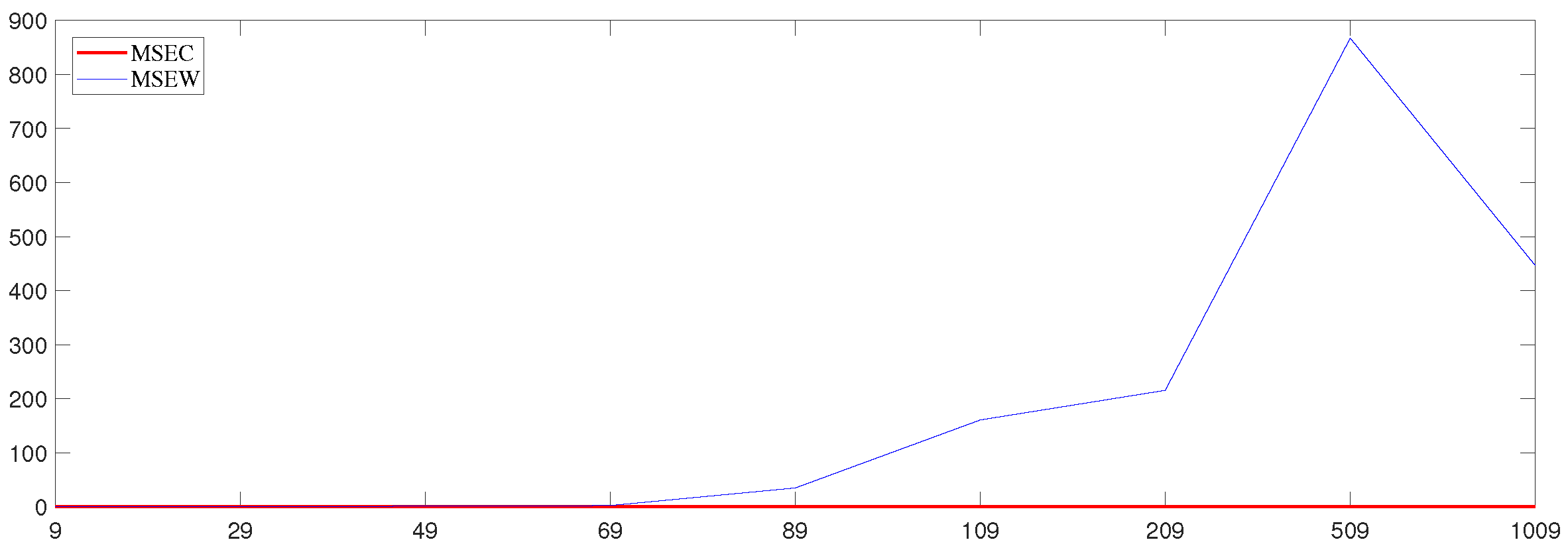
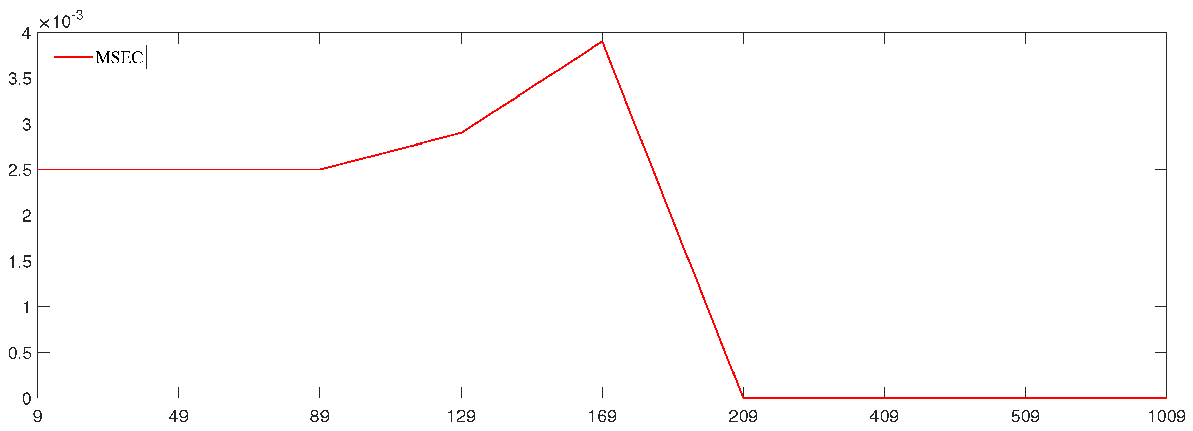
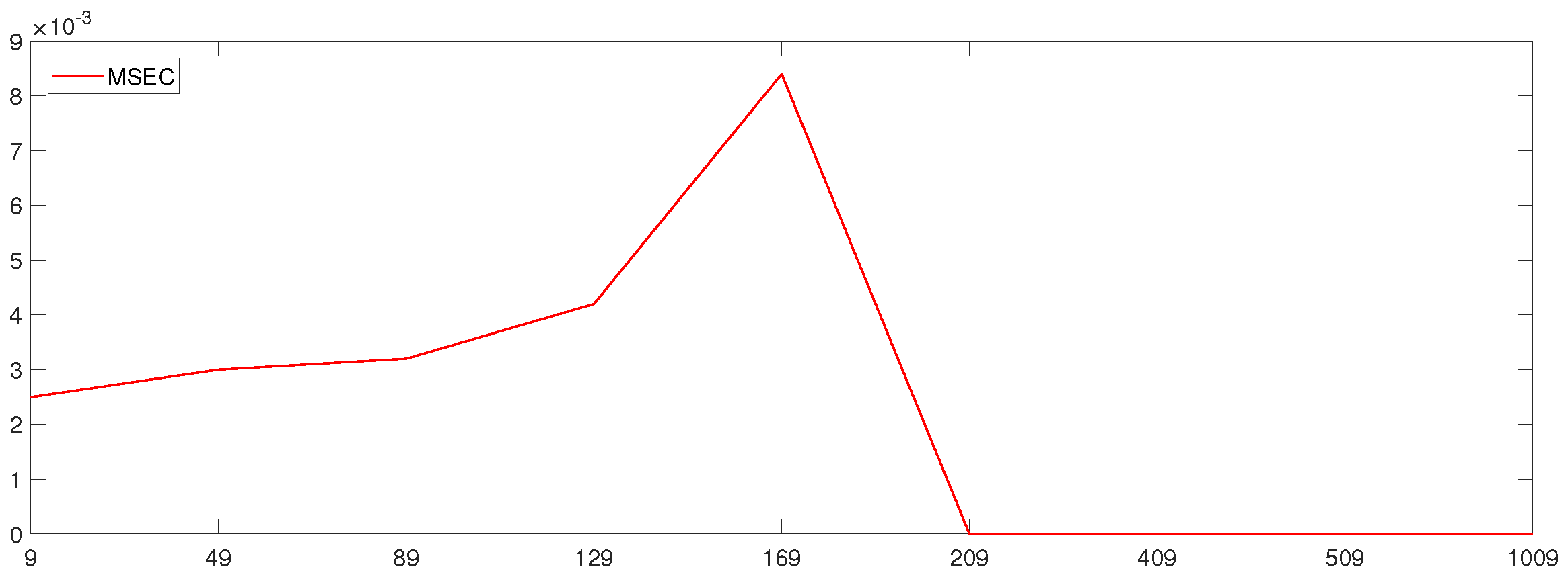
The simulation’s effect is expressed by the mean square error (MSE) of the parameter estimation, $\mathrm{MSE}={∥\widehat{\beta }-\beta ∥}^2$, where the sample sizes are $n=100,200$ and the dimensions are $p=9,29,49,69,89,109,129,169,209,509,1009$. The dimensions are taken from small to large by determining the value of the sample size. This was done, on the one hand, to compare with the results of Wang’s [17] study and, on the other hand, to study the simulation’s effect in the case of high dimensions ($p\gg n$). The effect of Wang’s study is expressed by the MSEW, and the effect of this paper is expressed by the MSEC.

According to the results in Table 1, the mean square error for this paper is slightly better than that of Wang’s study in the low-dimensional case, and the mean square error for this paper is slightly lower than that of Wang’s. The results are better in the high-dimensional case because the fitting effect of the augmented Lagrange multiplier method is better than that of the Lagrange multiplier method for high-dimensional data. For fixed values of p, the mean square error becomes larger with increasing $\sigma$, and the stability of the parameter estimation also becomes worse with the increase in $\sigma$. For fixed values of $\sigma$, the mean square error decreases with the increase in the dimensions p of the parameter. The method studied in this paper works better for parameter estimation in high-dimensional cases, and the higher the dimensionality, the better the stability of the parameter estimation.

A line plot of the mean square error for different variances was constructed with a sample size of 100 in order to specifically express the effects of this study (Figure 1, Figure 2 and Figure 3) and to provide a comparison with Wang’s results (Figure 4, Figure 5 and Figure 6).

Line plots of the mean square errors for different variances were constructed with a sample size of 200 to specifically express the effects of this study (Figure 7, Figure 8 and Figure 9) and for a comparison with Wang’s results (Figure 10, Figure 11 and Figure 12).

In these figures, it can be seen that the mean square error (MSEC) of the method studied in this paper is very small and is very close to zero in high dimensions. Moreover, the mean square error of this method is smaller than that of Wang’s method. Therefore, the method studied in this paper is more applicable in the case of high dimensions.

5.3. Application: Workers’ Wage Data Analysis

In order to test the algorithm proposed in this paper, we applied the algorithm to the practical problem of the analysis of workers’ wage data. The workers’ wage data were given by the 1985 Current Population Survey (CPS85) [29]. These data came from reality and are real. Moreover, the indicators of these data contained both quantitative data and classified data, so they were representative. In addition, the data were studied by other authors in the literature to facilitate comparison [30]. The data consisted of 534 samples of CPS85 personnel with 11 variables, which included wages and other characteristics of workers, such as gender, years of education, race, sex, marital status, years of work experience, occupational status, area of residence, and union membership. The wage level did not necessarily have a linear relationship with the years of work experience, so the importance of other variables for wages was mainly considered. The model was built as follows:

$$Y_i=\sum _{j=1}^{10}{X}_{ij}{\beta }_j+m\left(U_i\right)+{\epsilon }_i,$$

(30)

where $Y_i$ is the wage of the ith worker, $U_i$ is the number of years of experience of the ith worker, $X_{ij}$ is the jth variable of the ith worker, and ${\epsilon }_i\sim N(0,{\sigma }^2)$.

We describe the use of the method proposed in this paper to study the important factors that affect wages in this section. In order to reduce the absolute differences between wages, avoid the influence of individual extreme values, and satisfy the assumptions of the linear model as much as possible, a logarithmic transformation was required for the variable of wages.

During the experiment, it was necessary to select training samples and test samples. If the proportion of training samples was large, the model may have been closer to a model trained with all samples. However, if the proportion of test samples was small, the evaluation results would not be accurate enough. If the proportion of test samples was large, that could lead to a large difference between the evaluation model and the previous one, thus reducing the authenticity of the evaluation. In all samples, the division ratio for the training samples and test samples was typically 7:3 to 8:2. For large amounts of data, ratios of 9:1 or even 99:1 can be used. Based on the sample size of CPS85, 75 percent of the samples were selected as training samples, and the method in this paper was used for parameter estimation training. The remaining 25 percent of the samples were used as test samples to predict the wages of workers, and the predicted values were expressed in ${\widehat{y}}_i$. The test samples were used to evaluate the prediction ability of the model, and the prediction effect was evaluated with the median absolute error (MAE) and the standard error (SE).

The MAE attenuates the effects of outliers. The loss is calculated by taking the median of all absolute differences between the real and the predicted value.

$$\mathrm{MAE}=medain\left\{\right|y_1-{\widehat{y}}_1|,|y_2-{\widehat{y}}_2|,\cdots ,|y_n-{\widehat{y}}_n\left|\right\}.$$

(31)

The SE is a measure of the precision of data and reflects the degree of dispersion of a whole sample from the sample’s mean.

$$\mathrm{SE}=\sqrt{\frac{\sum {(y_i-{\widehat{y}}_i)}^2}{n}}.$$

(32)

The smaller the SE is, the greater the reliability of the prediction will be; otherwise, the reliability of the prediction is small.

The results are shown in

Table 2. The MAE and SE of predictions of workers’ wages.

Variables	Variable Description	MAE	SE
edu	Number of years of education	1.9777	0.0429
race	NW = 1, W = 0	0.7491	0.0861
sex	F = 1, M = 0	0.7526	0.0860
hispanic	Hisp = 1, NH = 0	0.7491	0.0861
south	S = 1, NS = 0	0.7491	0.0861
married	Married = 1, Single = 0	0.7521	0.0858
union	Union = 1, Not = 0	0.7491	0.0860
age	Age	1.9885	0.0517
sector	Clerical = 1, Const = 1, Manag = 1, Manuf = 1 Prof = 1, Sales = 1, Service = 1, Other = 0	0.7569	0.0857

.

As can be seen from the results in Table 2, the value of the MAE was small, indicating that the loss between the predicted and actual values of workers’ wages was lower. The values of the SE were all below 0.09, indicating that the prediction was reliable. In short, the MAE was low and the SE was small, so the parameter estimation method in this paper is relatively efficient.

6. Conclusions

The research in this paper considered a partially linear model with a restricted profile and used the least squares method to estimate the parameters with the purpose of minimizing the error. By constructing an augmented Lagrangian function under linear constraint conditions, the constrained optimization problem was transformed into an unconstrained optimization problem. The model was solved with the ADMM. The ADMM algorithm has the advantage that some large global problems can be solved by decomposing them into several smaller, more easily solvable local subproblems and then coordinating the solutions of the resulting subproblems to obtain the solution of the large global problem. The convergence of the algorithm was obtained by using the method of variational inequality. Through numerical simulations, the results showed that the method of this paper is suitable for parameter estimation in high-dimensional cases. Finally, this paper applied the algorithm to workers’ wage data from CPS85 and analyzed the important factors that affected wages.

In this paper, we used the ADMM algorithm to solve a high-dimensional partially linear model, and the effect was very good. The model in this paper is mainly for convex optimization problems. It can be used to solve other optimization problems, such as non-concave penalty optimization SCAD or MCP. This is a subject that will be studied further.

References

- Engle, R.F.; Granger, C.W.J.; Rice, J.; Weiss, A. Semiparametric estimates of the relation between weather and electricity sales. J. Am. Stat. Assoc. 1986, 81, 310–320. [Google Scholar] [CrossRef]
- Heckman, N.E. Spline smoothing in a partly linear model. J. R. Stat. Soc. Ser. (Methodol.) 1986, 48, 244–248. [Google Scholar] [CrossRef]
- Xu, H.X.; Chen, Z.L.; Wang, J.F.; Fan, G.L. Quantile regression and variable selection for partially linear model with randomly truncated data. Stat. Pap. 2019, 60, 1137–1160. [Google Scholar] [CrossRef]
- Chen, W. Polynomial-based smoothing estimation for a semiparametric accelerated failure time partial linear model. Open Access Libr. J. 2020, 7, 1. [Google Scholar] [CrossRef]
- Auerbach, E. Identification and estimation of a partially linear regression model using network data. Econometrica 2022, 90, 347–365. [Google Scholar] [CrossRef]
- Härdle, W.; Liang, H.; Gao, J. Partially Linear Models; Springer Science & Business Media: Berlin/Heidelberg, Germany, 2000. [Google Scholar]
- Tibshirani, R. Regression shrinkage and selection via the lasso. J. R. Stat. Soc. Ser. (Methodol.) 1996, 58, 267–288. [Google Scholar] [CrossRef]
- Ranstam, J.; Cook, J.A. LASSO regression. J. Br. Surg. 2018, 105, 1348. [Google Scholar] [CrossRef]
- Chetverikov, D.; Liao, Z.; Chernozhukov, V. On cross-validated lasso in high dimensions. Ann. Stat. 2021, 49, 1300–1317. [Google Scholar] [CrossRef]
- Xie, H.; Huang, J. SCAD-penalized regression in high-dimensional partially linear models. Ann. Stat. 2009, 37, 673–696. [Google Scholar] [CrossRef]
- Zeng, L.; Xie, J. Group variable selection via SCAD-L 2. Statistics 2014, 48, 49–66. [Google Scholar] [CrossRef]
- Gao, L.; Li, X.; Bi, D.; Xie, Y. Robust Compressed Sensing based on Correntropy and Smoothly Clipped Absolute Deviation Penalty. In Proceedings of the 2020 IEEE 3rd International Conference on Information Communication and Signal Processing (ICICSP), Shanghai, China, 12–15 September 2020; IEEE: Piscataway, NJ, USA, 2020; pp. 269–273. [Google Scholar]
- Zhang, C.H. Nearly unbiased variable selection under minimax concave penalty. Ann. Stat. 2010, 38, 894–942. [Google Scholar] [CrossRef] [PubMed] [Green Version]
- Breheny, P.; Huang, J. Penalized methods for bi-level variable selection. Stat. Its Interface 2009, 2, 369. [Google Scholar] [CrossRef] [PubMed] [Green Version]
- Ni, X.; Zhang, H.H.; Zhang, D. Automatic model selection for partially linear models. J. Multivar. Anal. 2009, 100, 2100–2111. [Google Scholar] [CrossRef] [PubMed] [Green Version]
- Chen, B.; Yu, Y.; Zou, H.; Liang, H. Profiled adaptive Elastic-Net procedure for partially linear models with high-dimensional covariates. J. Stat. Plan. Inference 2012, 142, 1733–1745. [Google Scholar] [CrossRef]
- Wang, X.; Zhao, S.; Wang, M. Restricted profile estimation for partially linear models with large-dimensional covariates. Stat. Probab. Lett. 2017, 128, 71–76. [Google Scholar] [CrossRef]
- Wei, C.H.; Wu, X.Z. Profile Lagrange multiplier test for partially linear varying-coefficient regression models. J. Syst. Sci. Math. Sci. 2008, 28, 416. [Google Scholar]
- Hestenes, M.R. Multiplier and gradient methods. J. Optim. Theory Appl. 1969, 4, 303–320. [Google Scholar] [CrossRef]
- Powell, M.J.D. A method for nonlinear constraints in minimization problems. Optimization 1969, 1, 283–298. [Google Scholar]
- Glowinski, R.; Marroco, A. Sur l’approximation, par éléments finis d’ordre un, et la résolution, par pénalisation-dualité d’une classe de problèmes de Dirichlet non linéaires. Revue française d’automatique, informatique, recherche opérationnelle. Anal. Numer. 1975, 9, 41–76. [Google Scholar]
- Boyd, S.; Parikh, N.; Chu, E.; Eckstein, J. Distributed optimization and statistical learning via the alternating direction method of multipliers. Found. Trends® Mach. Learn. 2011, 3, 1–122. [Google Scholar]
- Wahlberg, B.; Boyd, S.; Annergren, M.; Wang, Y. An ADMM algorithm for a class of total variation regularized estimation problems. IFAC Proc. Vol. 2012, 45, 83–88. [Google Scholar] [CrossRef] [Green Version]
- Yang, Y.; Sun, J.; Li, H.; Xu, Z. ADMM-CSNet: A deep learning approach for image compressive sensing. IEEE Trans. Pattern Anal. Mach. Intell. 2018, 42, 521–538. [Google Scholar] [CrossRef] [PubMed]
- Forero, P.A.; Cano, A.; Giannakis, G.B. Consensus-Based Distributed Support Vector Machines. J. Mach. Learn. Res. 2010, 11, 1663–1707. [Google Scholar]
- Glowinski, R.; Song, Y.; Yuan, X.; Yue, H. Application of the Alternating Direction Method of Multipliers to Control Constrained Parabolic Optimal Control Problems and Beyond. Ann. Appl. Math. 2022, 38, 115–158. [Google Scholar] [CrossRef]
- Joshi, S.; Codreanu, M.; Latva-aho, M. Distributed SINR balancing for MISO downlink systems via the alternating direction method of multipliers. In Proceedings of the 2013 11th International Symposium and Workshops on Modeling and Optimization in Mobile, Ad Hoc and Wireless Networks (WiOpt), Tsukuba, Japan, 13–17 May 2013; IEEE: Piscataway, NJ, USA, 2013; pp. 318–325. [Google Scholar]
- Gabay, D.; Mercier, B. A dual algorithm for the solution of nonlinear variational problems via finite element approximation. Comput. Math. Appl. 1976, 2, 17–40. [Google Scholar] [CrossRef]
- Berndt, E.R. The Practice of Econometrics: Classic and Contemporary; Addison-Wesley Publishing Company: Reading, MA, USA, 1991. [Google Scholar]
- Wang, X.; Wang, M. Adaptive group bridge estimation for high-dimensional partially linear models. J. Inequalities Appl. 2017, 2017, 1–18. [Google Scholar]
Figure 1.
Folding line plot of the mean square error for a variance of 0.5.
Figure 2.
Folding line plot of the mean square error for a variance of 1.
Figure 3.
Folding line plot of the mean square error for a variance of 2.
Figure 4.
Folding line plot of the compared mean square error for a variance of 0.5.
Figure 5.
Folding line plot of the compared mean square error for a variance of 1.
Figure 6.
Folding line plot of the compared mean square error for a variance of 2.
Figure 7.
Figure 8.
Figure 9.
Figure 10.
Figure 11.
Figure 12.