
Modified Whiteside’s Line-Based Transepicondylar Axis for Imageless Total Knee Arthroplasty

Department of Mechanical, Robotics and Energy Engineering, Dongguk University-Seoul, Seoul 04620, Korea
*
Authors to whom correspondence should be addressed.
Mathematics 2022, 10(19), 3670; https://doi.org/10.3390/math10193670
Submission received: 7 September 2022
/
Revised: 28 September 2022
/
Accepted: 1 October 2022
/
Published: 7 October 2022
(This article belongs to the Special Issue Numerical Simulation in Biomechanics and Biomedical Engineering-II)
Abstract
:One of the aims of successful total knee arthroplasty (TKA) is to restore the natural range of motion of the infected joint. The operated leg motion highly depends on the coordinate systems that have been used to prepare the bone surfaces for an implant. Assigning a perfect coordinate system to the knee joint is a considerable challenge. Various commercially available knee arthroplasty devices use different methods to assign the coordinate system at the distal femur. Transepicondylar axis (TEA) and Whiteside’s line are commonly used anatomical axes for defining a femoral coordinate system (FCS). However, choosing a perfect TEA for FCS is trickier, even for experienced surgeons, and a small error in marking Whiteside’s line leads to a misaligned knee joint. This work proposes a modified Whiteside’s line method for the selection of TEA. The Whiteside’s line, along with the knee center and femur head center, define two independent central planes. Multiple prominent points on the lateral and medial sides of epicondyles are marked. Based on the lengths of perpendicular distances between the multiple points and central planes, the most prominent epicondyle points are chosen to define an optimal TEA. Compared to conventional techniques, the modified Whiteside’s line defines a repeatable TEA
1. Introduction
The knee joint is the largest joint in the human body. Osteoarthritis-induced wear and tear of the articulating surfaces of the knee causes discomfort to the patient [1]. Arthroplasty is considered to be the permanent solution to treat the most severe knee arthritis [2]. Surgeons perform total knee arthroplasty (TKA) relying either on an imaging technique like ultrasound [3] or an imageless computer-based technique [4]. The computer-assisted TKA is becoming popular, because most of the alignment work is done by computers; hence, the transplanted joint is expected to be accurately aligned, with quicker recovery time, due to minimal incision [5]. The computer-assisted TKA device consists of software that takes some anatomical points as input. The marking system of these anatomical points usually relies on an infrared, laser, or electromagnetic pulses emitter, and reflectors paired with an optical camera to obtain the real-time position of the marked point [6,7,8].
The software constructs a virtual coordinate system for the knee to undergo arthroplasty, and based on the coordinate system, it guides the surgeon to prepare the bone surface for implant. The coordinate system can be assigned by different methodologies, for example, the transverse axis at the distal femur for assigning a femoral coordinate system (FCS) can be obtained by fitting a circle, a sphere, or a cylinder in the articulating surfaces of the distal femur, and using the center of the fitted geometry, the transverse axis is assigned [9,10]. Another approach is to join the most prominent points on the lateral and medial epicondyles to construct an anatomical transepicondylar axis (aTEA) [11]. Similarly, a surgical transepicondylar axis (sTEA) can be defined by joining the lateral epicondyle and medial sulcus [12]. In some cases, the posterior condylar axis (PCA) being in front of the surgeon can be easily used to define the transverse axis [13]. PCA and sTEA are parallel to each other, and perpendicular to the anterior posterior axis (AP axis) or Whiteside’s line [14,15]. Whiteside’s line is defined by using the deepest part of the patella groove (PG) anteriorly and the center of intercondylar notch (N) posteriorly [16]. sTEA is considered to be a standard to set the rotational alignment for TKA [17,18]. However, some studies have compared the sTEA and aTEA for their ability to be chosen as a transverse axis for FCS. For example, Tanavalee et al. studied the CT scans of 55 osteoarthritic knees considering both sTEA and aTEA, and they concluded that aTEA is near perpendicular to the AP axis and more reliable for rotation alignment compared to sTEA [19]. In the same year, Yoshino et al. examined 48 patients eligible for TKA and found that the medial sulcus was detectable in only one-fifth of the severe osteoarthritis cases; for less severe cases, it was detectable in half of the cases [20]. Hence, it was concluded that the chances of detecting the medial sulcus decrease with an increase in the severity of osteoarthritis.
Deterioration of PCA in severe osteoarthritis makes it less favorable for the selection of the transverse axis [20]. Whiteside’s line being a smaller landmark leads to rotational error of up to 10°, even for small uncertainties [21]. It is a well-known fact that alignment error >3° from the natural alignment of the knee leads to quick wear and discomfort of the patient, and finite element analysis can accurately predict initial stability of an implant; however, the computational cost increases [15,22,23]. The sTEA, being an inconsistent landmark [24], leaves only aTEA to be a reliable choice for assigning the FCS and setting the rotational alignment of the implant [19,25]. Malrotation alignment leads to instability of implant, the discomfort of the patient, patella maltracking, and quick wear of inserted polyethylene [26]. So, the TKA is sometimes required to be revised. Fehring et al. summarized the 15-year data of revised TKA cases and found that 41% of the cases showed conditions related to rotational malalignment [27]. Another similar case study of 1632 revised TKA cases showed that 42% of the cases were linked with wear of the insertion and instability of the implant [28]. Dalury et al. also investigated the reasons why TKAs are revised, based on the analysis, 48% of the cases were linked with the symptoms attached to rotational malalignment [29]. Choosing a perfect aTEA is not always possible, which leads to rotational malalignment. Stoeckl et al. invited a team of four experienced surgeons to mark six cadaveric human legs. Skin and soft tissues were removed, and surgeons had to pick the most prominent point on lateral and medial epicondyles using an optical navigation system under perfect laboratory conditions. Each surgeon marked aTEA for three consecutive days; 144 points were marked by all the surgeons. Excluding extreme values, the selected points were distributed in an area of 298 mm2 on the medial and 278 mm2 on the lateral side of the bone. Using the extreme values of the marked area, a maximum of 8° of internal rotation was calculated (3° allowed) [30]. Another study investigating the reproducibility of aTEA, where eight surgeons marked lateral and medial epicondyles on Thiel-embalmed cadaver specimens, shows the distribution of lateral and medial epicondyles on an area of 116 and 102 mm2, respectively [31]. A team of another five surgeons studied the effect of errors in registering anatomical points on five cadavers for five days. Key anatomical points, including lateral and medial epicondyles, were intentionally marked wrong. The wrong registration of lateral and medial epicondyles led to an error in rotational alignment ranging from 11.1° external to 6.3° internal rotation [32]. Similarly, there are various studies in which the errors are either intentionally added, or induced due to human error, by the repetitive marking of points during a course of time. The objective of such studies is to show the effect of errors on the rotational alignment of TKA [32,33,34,35,36].
To reduce the errors caused by choosing a single point, bone morphing or selection of multiple points on the landmark have been reported in the literature. For example, Liu et al. marked a group of points and fitted an algorithm to choose the optimal point for defining TEA [37]. Perrin et al. studied the reproducibility of implant positioning in TKA using both morphing and conventional single-point selection techniques, and found the bone morphing technique to be more repeatable [38]. A system using bone morphing relies on a database gathered by CT scans from a large number of patients supplied by the device manufacturers. Once multiple anatomical points are registered by the surgeon, the algorithm finds the bone model that best fits the marked points [39]. Instead of model fitting, statistical shape models of the bone can be fitted in a marked cloud of points. The bone morphing requires the surgeon to carefully mark the entire distal femur. This is a time-consuming job, and error at this stage can lead to the failure of TKA [40]. This is because bone morphing requires model fitting, which increases the computational cost, and hence, the cost of TKA.
From the above literature review, it can be concluded that, since the beginning of computer-based TKA, researchers have relied on an individual anatomical axis to set the transverse axis of FCS. However, the reported outcomes are not repeatable and certain. Thus, it is necessary to investigate the repeatability and accuracy of a transverse axis defined by the combination of more than one anatomical axis. Currently, the aTEA is the most reliable transverse axis for FCS; however, it is not a repeatable axis. This work proposes a modified Whiteside’s line, which combines the Whiteside’s line and aTEA to define a repeatable transverse axis. Moreover, this method can also be added to the existing TKA devices just by their software upgradation. The rest of the paper is organized as follows: Section 2 reviews the generalized method to define FCS, the tibial coordinate system (TCS), and presents the proposed modified Whiteside’s line. Section 3 describes the CAD and experimental setup. Section 4 presents and interprets the results, while Section 5 concludes the work.
2. Methodology
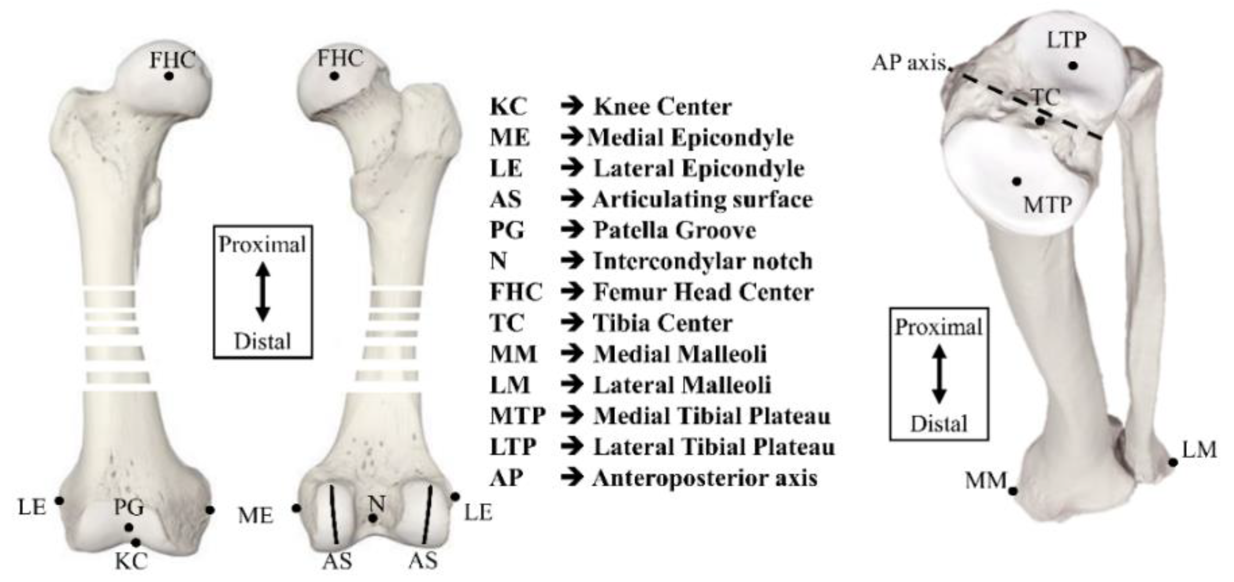
The imageless TKA device consists of two components: (a) a sensing system containing a pair of optical sensors coupled with an infrared camera, to capture anatomical points marked by the surgeon; and (b) an algorithm to utilize the surgeon-marked points for the construction of a coordinate system to prepare the bone surfaces for implant placement. The coordinate systems developed virtually at the distal femur and proximal tibia are referred to as FCS and TCS, respectively. The nomenclature of anatomical points to perform an imageless TKA is marked on open-source bone models, as shown in Figure 1 [41]. In the following section, a generalized procedure adopted to create FCS and TCS is explained first. Later, the modified Whiteside’s line technique is developed.
2.1. Defining the Procedure for a Coordinate System
The algorithm to assign FCS and TCS is programmed in MATLAB. The anatomical points shown in Figure 1 are the required inputs for this algorithm. FCS and TCS are independent of each other.
2.1.1. Femoral Coordinate System
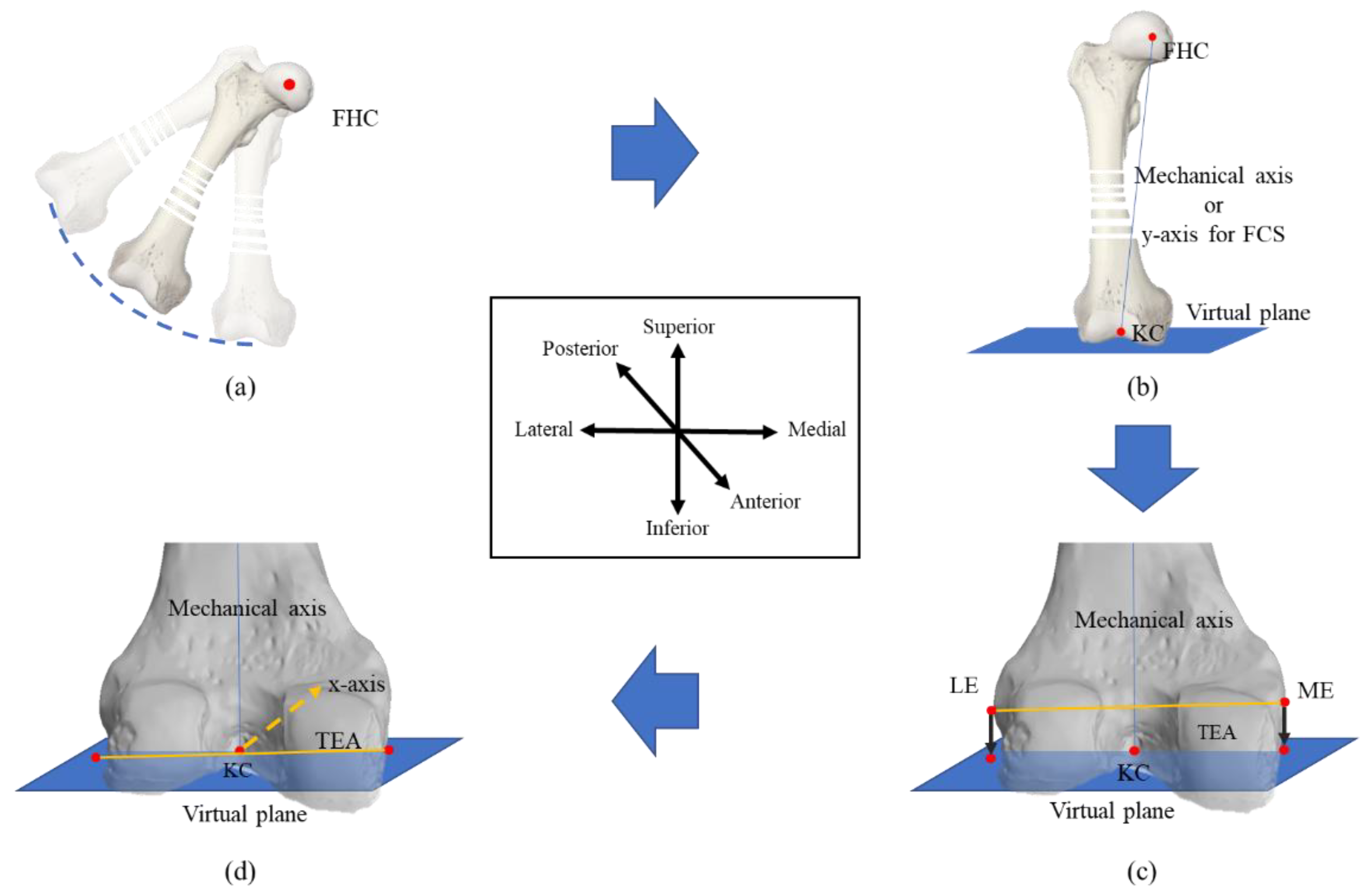
Assignment of FCS requires the identification of a knee center (KC), which becomes the origin of FCS. For this work, the femur mechanical axis is taken as the y-axis. The z-axis is marked between the lateral and medial sides. The x-axis is obtained by the cross product of the earlier marked axes and lies between the anterior and posterior of the body. Figure 2 shows a generalized four-step approach defined on an open-source [42] model.
Step 1: A fixed sensor is attached at the distal femur. Keeping the hip stationary, the circular motion of the femur allows the attached sensor to capture the surface of a sphere. A sphere-fitting algorithm fits an approximate sphere to the marked surface. The center of the sphere is the femur head center (FHC), as shown in Figure 2a. For the proposed work, a fast geometric fit algorithm for sphere is used because of its computational efficiency [43].
Step 2: During surgery, KC is marked by the surgeon. Currently, KC is taken above the center of the intramedullary canal hole, which is approximately 3 mm medial to the center of the femoral groove and 10 mm anterior to the posterior condylar ligament [44]. Figure 2b shows the process where FHC and KC define the femur mechanical axis and y-axis for FCS. A virtual plane parallel to a sagittal plane is created using Equation (1) for the projection of the transverse axis to be defined in step 3 [45]:
where, a, b, and c are the coefficients of the femur mechanical axis, and d is the distance between origin and plane.
Step 3: The transverse axis can be marked in several ways, for example by aTEA, Whiteside’s line, and sphere fitting [9,10,11]. Once anatomical points on the distal femur are finalized by the surgeon, these points are projected onto the defined virtual plane, as shown in Figure 2c [46]. This projection ensures the orthogonality of the mechanical and transverse axes. Equations (2)–(4) represents the generalized equation for point projection:
where (x0, y0, z0) are the coordinates of the point to be projected on the plane; are the coordinates of a projected point; , , and are the components of the normal vector of plane calculated in Equation (1); and is the parameter such that the projected point is on the plane and line at the same time.
In the case that the anatomical points to accurately mark the transverse axis have deteriorated, the third axis is marked by Whiteside’s line, since it is almost perpendicular to the epicondylar axis as calculated by Middleton and Palmer [15]; the average angle between Whiteside’s line and the epicondylar axis is 91°.
Step 4: Once two axes are finalized, the cross product between the femur mechanical axis and the transverse axis or Whiteside’s line completes the assignment of FCS, as shown in Figure 2d:
where ‘⨯’ represents the cross product.
2.1.2. Tibial Coordinate System
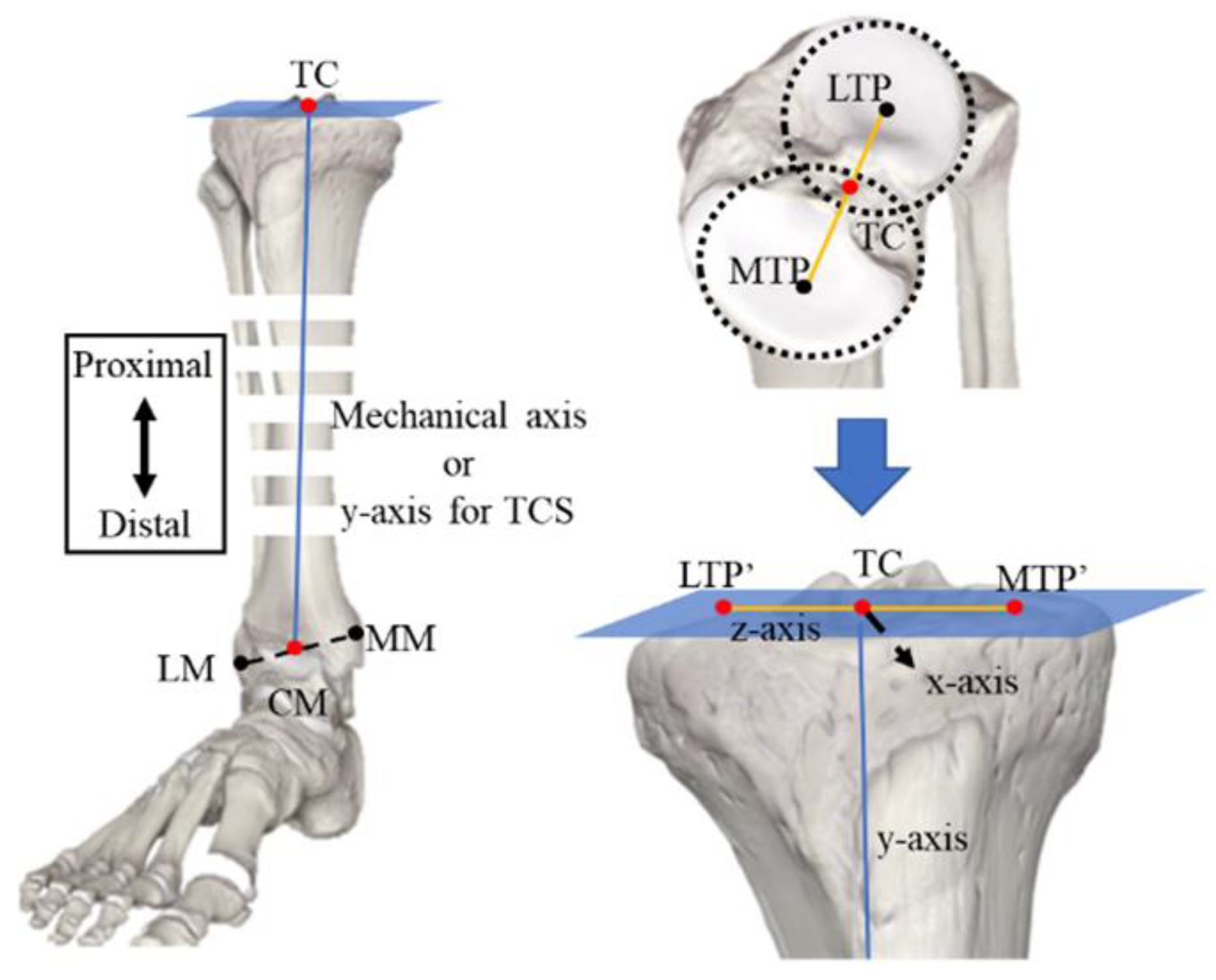
The contribution of this work is related to the FCS only. The generalized method to assign TCS is explained because the algorithm used to define FCS can also define TCS, with change in only the first step. Figure 3 shows the steps carried out to define TCS [47]:
Step 1: The center of the malleoli/ankles is obtained by marking the lateral and medial malleoli. The midpoint of the axis defined by the coordinates of the lateral malleolus (LM) and medial malleolus (MM) is the center of malleoli (CM), which is not an exact average of LM and MM, but can be calculated by the following formula [48]:
The tibia center (TC) is obtained by fitting a circle in the outer surfaces of the lateral tibial plateau (LTP) and medial tibial plateau (MTP); the midpoint of the line joining the centers of circles will define the TC. Then, TC and CM define the mechanical axis (y-axis) for TCS. For orthogonality of TCS, a plane is defined using TC and CM for the projection of MTP and LTP, using Equations (2)–(5).
Step 2: The centers of circles fitted in LTP and MTP define the z-axis. These centers are projected onto the virtual plane to create a z-axis orthogonal to the y-axis.
Step 3: The cross product between the z-axis and y-axis completes the definition of TCS.
2.2. Modified Whiteside’s Line
Whiteside’s line and aTEA are the most common transverse axes being used in commercial TKA devices because these anatomical axes are reported in clinical studies to be (almost) perpendicular to each other [15]. However, due to the small length of the Whiteside’s line, a minute registration error leads to a large orientation error [21]. On the other hand, choosing an exact bony point to define an aTEA is nearly impossible, even under ideal conditions [30,31]. Utilizing the anatomical properties of the Whiteside’s line and aTEA, a modified Whiteside’s line method can be applied to define the transverse axis for FCS in a novel way. This method relies on the orthogonality of the Whiteside’s line and aTEA, and the fact that the distance between the boniest points and a plane defined by the Whiteside’s line will be the largest perpendicular distance among all points on the lateral and medial epicondyles.
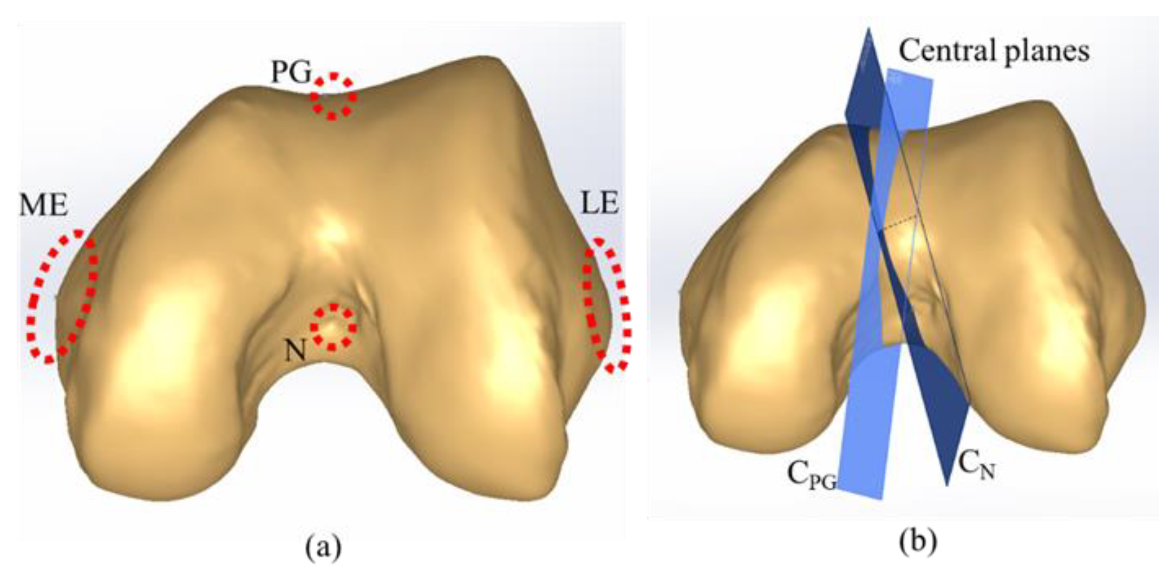
The modified Whiteside’s line requires marking multiple points on the lateral and medial sides of the epicondyle, referred to as a cloud of points. Figure 4a shows the position of clouds, N, and PG. This proposed algorithm is programmed in MATLAB. Within the algorithm, the center of N, KC, and FHC and PG, KC, and FHC defines two independent central planes CN and CPG, respectively, as shown in Figure 4b. The perpendicular distance between each point of the lateral cloud and CN plane is calculated using Equation (7) [49].
where (xo, yo, zo) are the coordinates of the point and (a, b, c) are the components of the normal vector.
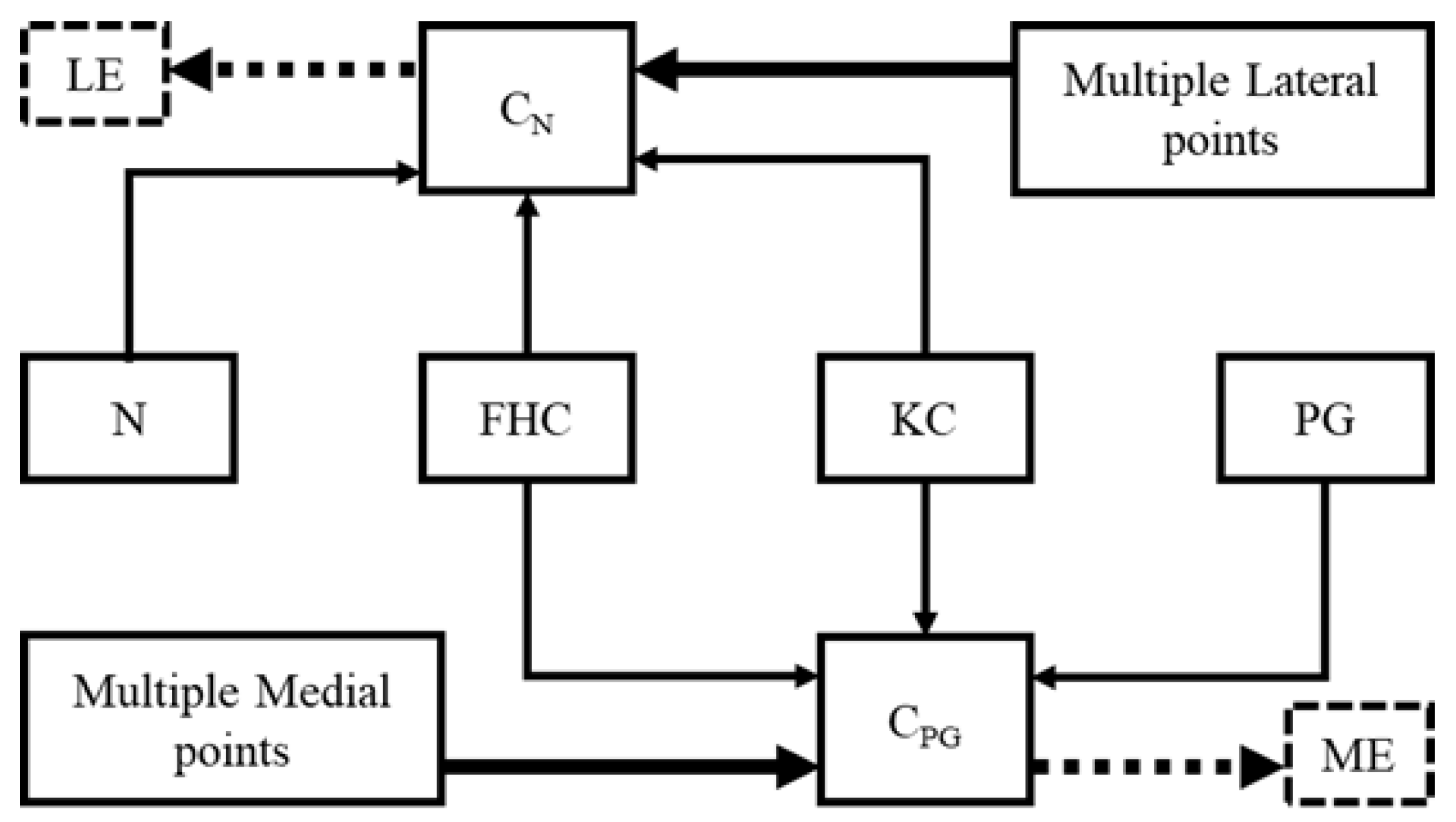
Similarly, the perpendicular distance between each medial point and CPG is calculated. The points corresponding to the largest perpendicular distances on each side are selected to define the aTEA. The chosen points define a repeatable aTEA, because the highest point will always have the largest perpendicular distance. Algorithm 1 and Figure 5 describe the working principle of the MATLAB algorithm. The remaining procedure to define FCS is carried out as usual.
| Algorithm 1: Modified Whiteside’s line for FCS |
| Input: KC, FHC // Chosen be probe sensor MPoints, LPoints // A cloud of points on the lateral and medial sides Output: xaxis, yaxis, zaxis // FCS yaxis := (FHC – KC) // A plane normal to the y-axis and passing through KC VP := ∏ (yaxis, KC) CN := ∏ (N, KC, FHC) CPG := ∏ (PG, KC, FHC) // Function 1: Selection of prominent point from MPoints ME := Function 1 (CPG, MPoints) LE := Function 1 (CN, LPoints) // Function 2: Projection of prominent point on the virtual plane MEProjected := Function 2 (ME, VP) LEProjected := Function 2 (LE, VP) zaxis := (MEProjected – LEProjected) xaxis := yaxis x zaxis chosen point := Function 1 (plane equation, cloud points) for i := 1 to # cloud points ith cloud point := (x, y, z) ith cloud point, 4th column := |ax+by+cz+d|/sqrt(a2 + b2 + c2) endfor j := find indices of max(ith cloud point, 4th column) chosen point := jth cloud point endFunction 1 Projected point := Function 2 (point, plane) point := (xo, yo, zo) x := xo + at; y := yo + bt; z := zo + ct; substitute (x, y, z) in plane and solve for “t” Projected point := substitute “t” in (x, y, z) endFunction2 |
3. Experimental Setup
3.1. CAD Model
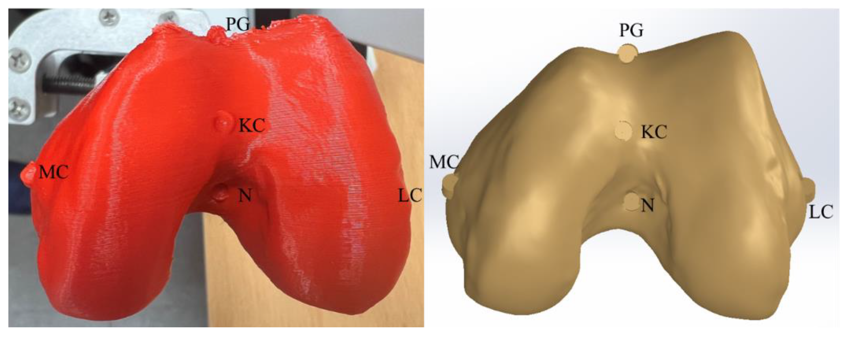
During the actual surgery, all the anatomical points are recorded via either fixed or movable sensors. For this work, an open-source CT scan of a 44-year-old human bone is used. The weight and height of the patient are 85 kg and 185 cm, respectively [42]. All the anatomical points, including KC, Whiteside’s line, and the highest points on the lateral and medial epicondyles (LE and ME) are marked in CAD. An alternative for this work, in contrast to real surgery, is that during surgery, FHC is obtained by the circular motion of the femur with a fixed sensor attached to the distal femur; however, for this experiment, FHC is obtained in commercial CAD software (Solidworks). Once all the points are marked, the bone model is printed, and anatomical points are captured, using a sensing system for experimental verification. During 3D printing, the bone model was linearly scaled down by 10% to print within the printing bed size of the 3D printer. Due to this downscaling, the size of the CAD model is larger than that of the printed bone. This change in size will not affect the results, as each axis of the FCS will be normalized. Figure 6 shows the marked CAD and 3D-printed models.
3.2. Sensing System
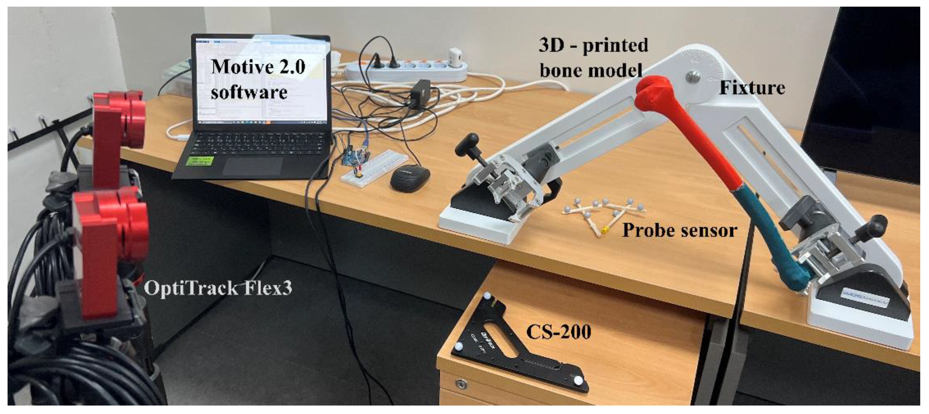
The sensing system consists of a pair of OptiTrack Flex 3 cameras coupled with Motive 2.0 software (OptiTrack, Corvallis, OR, United States). This software requires a CS−200 calibration square and a probe sensor to capture the coordinates of different anatomical points. Figure 7 shows the experimental setup including infrared (IR) camera (OptiTrack Flex-3), fixed tracker (CS−200), 3D-printed bone model, bone fixture, and probe sensor. This passive system relies on the IR beam emitted by the OptiTrack camera. The spherical markers attached to the fixed and probe sensors reflect the IR beam. Motive 2.0 processes the reflected beam to provide the instantaneous position of the probe sensor with respect to the CS−200.
The CS−200 acts as a global coordinate system (GCS) for the probe sensor measurements. In this work, the data from the sensing system will be validated with CAD data. Since the GCS for the CAD model and sensing system are different, the CAD global coordinate system (CAD−GCS) is shifted to FCS in CAD, and the CAD-femoral coordinate system (CAD−FCS) acts as a common coordinate system (C−CS). To check the accuracy of the sensor measurement, FCS is defined on the 3D-printed bone, and a homogeneous transformation matrix (HTM) is created using Equation (8) [50].
where “A” represents a base frame with respect to which frame “B” is defined. is a 3 × 3 rotation matrix to express the orientation of “B”, and is a position vector between the origin of “A” and “B”. Once the sensor-measured anatomical points are transformed into the sensor-femoral coordinate system (S−FCS) frames using Equation (9), the accuracy of the sensing system can be checked against CAD-measured anatomical points [51]:
where is the inverse HTM. represents the position of any anatomical point in the sensor-global coordinate system (S−GCS) that is to be transformed into S−FCS. The coordinates of anatomical points in CAD−FCS can either be obtained directly in Solidworks or by repeating the procedure used to obtain the anatomical points in S−FCS by defining an HTM.
4. Results and Discussion
This section is divided into three parts. First, the results of the sensing system are compared with the CAD results to verify the authenticity of the experimental setup. The repeatability of current techniques to assign transverse axis is checked in Solidworks. In the end, the proposed technique is verified in the CAD and experimental environments.
4.1. Validation of the Sensing System with CAD Results
The points used to define the anatomical axes for FCS are marked on the CAD model before 3D printing, as shown in Figure 6. Table 1 gives each anatomical point in CAD−GCS. These points include KC, FHC, ME, and LE to define the HTM, and N and PG to define the two central planes CN and CPG, respectively. The unit vectors of CAD−FCS in CAD−GCS construct the rotation part, and the position of KC in GCS completes the HTM given in Equation (10):
Equation (9) and transform CAD−GCS anatomical points into CAD−FCS. Table 1 gives the transformed anatomical points.
Similarly, an HTM from S−GCS to S−FCS is defined following the same procedure as for CAD−GCS to CAD−FCS. Table 2 shows the S−GCS coordinates of each anatomical points being used to define an HTM given in Equation (10). Additionally, N and PG will be used for defining CN and CPG planes, respectively. Furthermore, by using Equations (9) and (10), S−GCS anatomical points transformed into S−FCS are also shown in Table 2.
4.2. Repeatability Challenge in Conventional Techniques
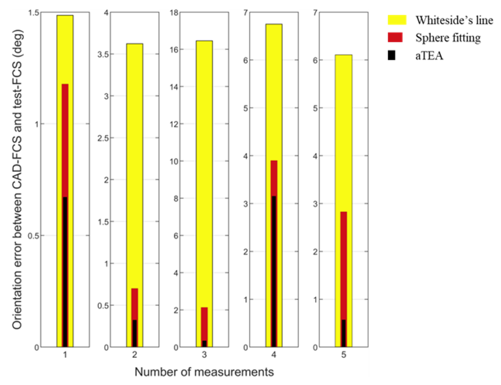
To verify the limitations of Whiteside’s line, aTEA, and sphere fitting as reported in the literature, FCS is developed using each axis one at a time. Each anatomical axis is marked five times by viewing the distal femur from a different view. For example, LE and ME are marked by viewing the distal femur from top, bottom, anterior, posterior, and isometric views. In each view, the apparent highest points on the lateral and medial sides of the epicondyle are marked to define aTEA. Similarly, the sphere-fitting curve and Whiteside’s line are marked to define the “test-FCSs”. Figure 8 shows the orientation error between CAD−FCS and each test–FCS for five measurements of each method. It is observed that a small change in marking Whiteside’s line led to large changes in orientation, and aTEA is close to CAD−FCS for two of the measurements. Similar results were observed by Victor et al. during a study of 12 cadaveric specimens [21]. Whiteside’s was concluded to be the least consistent axis, with errors up to 11.67°. Similarly, the maximum error for aTEA was 6.16°.
The results of the sphere-fitting line in between the aTEA and Whiteside’s method are discussed. Sphere or cylinder fitting defines an accurate axis only when a fitting is done between (10 and 110)° of flexion [52,53]. For this experiment, the sphere is fitted between a full articulating surface, (0 to 110)°, (10 to 100)°, (0 to 100)°, and (10 to 110)° of flexion. Overall, it is observed that the conventional methods are not repeatable.
4.3. Modified Whiteside’s Line—CAD Results
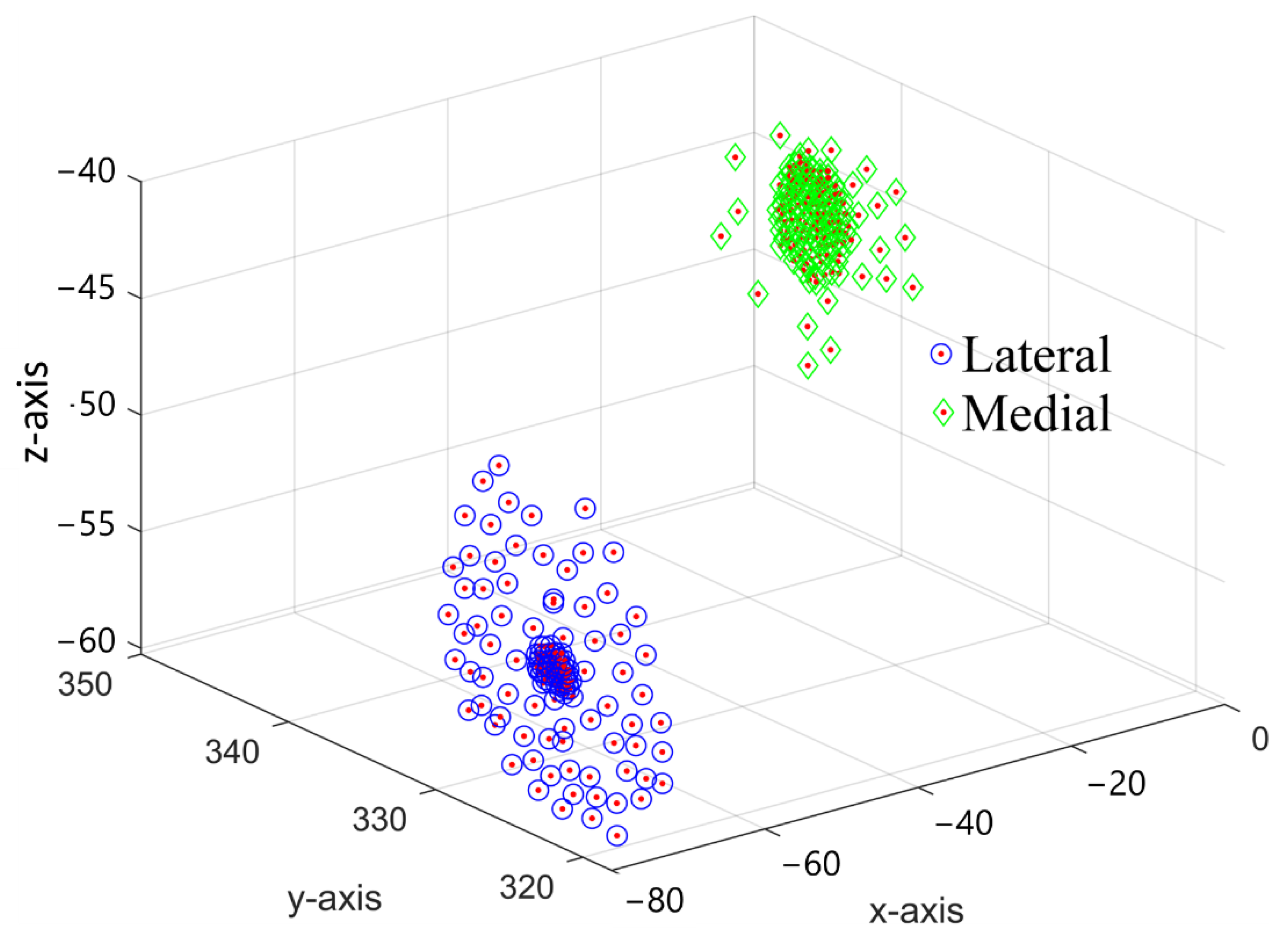
First, the proposed technique is tested using CAD data. Multiple points on the lateral and medial sides of the epicondyle are marked. The algorithm will choose the highest LE and ME points from the marked points. A total of 141 points were marked on the lateral side, and 145 points were marked on the medial point. Around the apparent highest lateral and medial points, the points that are also printed on the 3D bone model, dense points were marked with their surface-to-surface distance of no more than 0.25 mm, as shown in Figure 9. The spread of the cloud was 8.27 mm on the lateral side and 7.62 mm on the medial side. Similarly, 66 points in PG and 63 points in N with cloud spread of 4.15 mm and 5.35 mm, respectively, were marked for an algorithm to define CPG and CN, using one point at a time.
Based on the marked points, the algorithm defined FCS using each point, and compared its orientation with FCS defined by aTEA. For example, first, a constant LE marked on the bone is used while calculating ME by the proposed method. To get a new ME, each point marked in PG along with KC and FHC is used to define the CPG plane. Based on the largest perpendicular distance, ME is chosen from the medial cloud. FCS is defined using the obtained points, and its orientation is compared with reference FCS defined using the marked aTEA, as described in Figure 6. Since the y-axis is the same in both FCSs, the angle between the z-axis is measured to obtain the orientation error. Once all points are used to define CPG, ME is kept constant, and points marked in N are used to define CN, to find the LE from the lateral cloud. Table 3 compares the orientation error between the FCSs obtained by Whiteside’s line, aTEA, and the proposed modified Whiteside’s line. The orientation error is measured by defining an anatomical point 3 mm away from its ideal position. To measure the error, first FCS is defined using an ideal anatomical point, then the anatomical point is marked with 3 mm of error in a lateral or medial direction to define a second FCS. Finally, the orientation between the first and second FCSs is measured to check the effect of 3 mm error on that anatomical axis.
For the Whiteside’s line, it is observed that 3 mm error in PG in the lateral direction caused a 6.73° deviation of FCS, while in the medial direction, 5.77° error was observed. For N in the lateral and medial directions, 3.36° and 5.50° error was observed, respectively. For an aTEA lateral side, 3 mm in anterior and posterior directions caused 2.33° and 2.49° deviation, respectively. Similarly, for the medial side, 2.37° and 2.47° deviations were observed. Before testing the modified Whiteside’s line, it was made sure that the anatomical point coordinates used for testing aTEA are included in lateral and medial clouds; also, the CN and CPG were defined using the same points that were used to define the Whiteside’s line. With the proposed method for 3 mm off of the marked PG position, 0.72° and 1.33° deviations were observed on the lateral and medial sides, respectively. For N, it was 0.64° and 2.06° on the lateral and medial sides, respectively. The maximum orientation error using the proposed method is 3.22° when PG is marked 19.80 mm away in a lateral direction and 5.54° when PG is 8.73 mm in the medial direction. Similarly, for N, maximum orientation error of 2.50° was observed at 19.20 mm in a lateral direction and 5.48° when N moved 12.75 mm in the medial direction. It is also observed that within the radius of 2.1 mm around the actual N, the mean orientation error was 0.4197°. The mean orientation error around 1.76 mm radius of PG was 0.3566°.
4.4. Modified Whiteside’s Line—Experimental Results
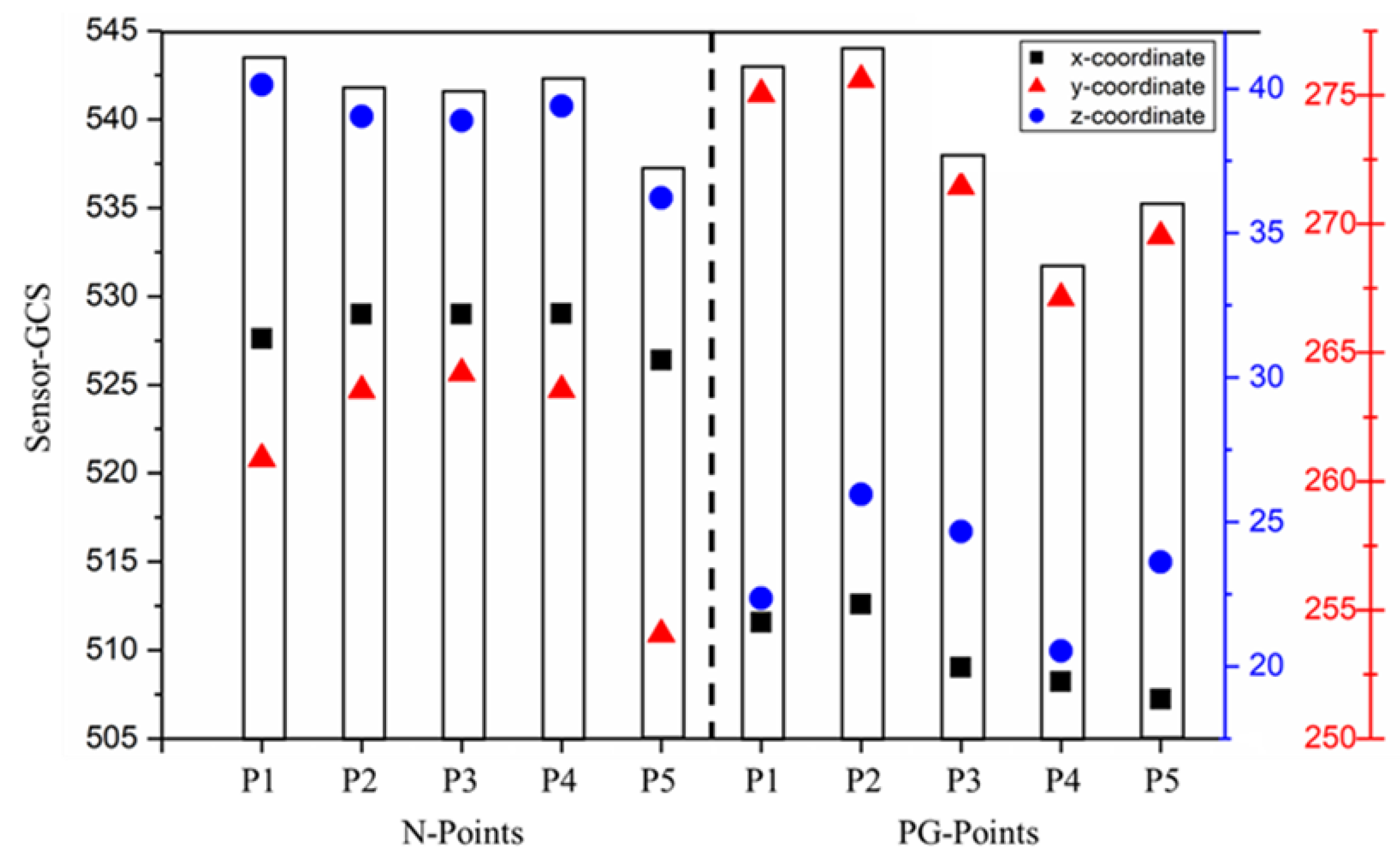
For experimental validation, five points were marked in N and five points in PG using the probe sensor. The probe sensor captures 30 frames per second. For lateral and medial clouds, epicondyles were painted with a probe sensor for five seconds on each side to obtain 150 points in each cloud. The number of points added in the medial and lateral clouds are directly proportional to both the accuracy of the femoral implant and the surgery time. Figure 10 shows the sensor-marked PG and N points. While marking the N points, it was observed that marking the N point is easy compared to PG, as the N lies inside the notch, and is easy to identify. On the other hand, PG lies inside the curve with large curvature, so it needs to be marked carefully. However, during surgery, PG lies in front of the surgeon, so it can be accurately marked by an experienced surgeon. For experimental validation, the FCS is defined using the printed LE and ME points, as shown in Figure 6. Another FCS is defined by keeping LE the same as printed on the bone, and ME is defined using the modified Whiteside’s line method. The error is a measure of the difference in orientation of both FCSs. Similarly, once all PG points are used to find ME, LE is chosen from the lateral cloud using all N points, one at a time.
Table 4 shows the orientation error for different points. PG and N points were marked around the marked PG and N points in all directions. With the modified Whiteside’s line for the PG case, a minimum error of 0.3441° and a maximum error of 1.9197° were observed. The mean error and standard deviation for five measurements were 0.8481° and 0.6414°, respectively. For the N case, the minimum and maximum errors were 0.4586° and 0.9684°, respectively. The mean error and standard deviation for five measurements were 0.7566° and 0.1848°, respectively. These results show that the modified Whiteside’s line produces near repeatable aTEA. Additionally, for conventional methods, as the error in the registration of anatomical points increases, the orientation error increases proportionally. On the other hand, the proposed method picks LE and ME from cloud points, so it defines a more reliable and repeatable TEA.
5. Conclusions
The accuracy of imageless TKA relies on the anatomical points used to develop the FCS and TCS, as these coordinates are used to prepare the bone surfaces for an implant. Currently, imageless TKA devices use the femur mechanical axis as one of the axes of the FCS. The assignment of a transverse axis between lateral and medial sides is a critical task. The aTEA, Whiteside’s line, and sphere-fitting line approach in articulating surfaces are three popular methods to assign the transverse axis; however, with a change in viewing angle, the repeatability of each of these anatomical axes is disturbed. In this work, a modified Whiteside’s line approach is proposed that provides an adaptable technique to choose a near repeatable aTEA. This technique requires a cloud of points on the lateral and medial sides of epicondyles, and two central planes: CN—defined using N, KC, and FHC; and CPG—defined by PG, KC, and FHC. Based on the perpendicular distances between cloud points and CN and CPG, the highest points on the lateral and medial epicondyles are selected to define the aTEA. The proposed technique has been verified in Solidworks software, and experimentally by using the OptiTrack sensing system. Around 140 points were marked for each cloud, and 60 points were respectively marked for PG and N. FCS is defined using each PG and N point one at a time. The repeatability of the proposed method is verified by measuring the orientation of each developed FCS against a standard FCS.
Furthermore, the repeatability of the modified Whiteside’s line, aTEA, and Whiteside’s line are compared at 3 mm registration error. It is observed that the Whiteside’s line is the most unrepeatable axis, with orientation error up to 6.73°; with a 3 mm error in an aTEA axis, the maximum orientation error was 2.49°. The modified Whiteside’s line produced repeatable results with a maximum orientation error of 1.33° on PG and 2.06° on N sides. Additionally, with the conventional techniques, increase in registration error always increases the orientation error; however, with the proposed method, for PG with 19.80 mm and 8.73 mm errors in the lateral and medial directions caused only 3.22° and 5.54° orientation errors, respectively. For N cases, 2.50° and 5.48° of error were observed with registration errors of 19.20 mm and 12.75 mm in the lateral and medial directions, respectively. Additionally, within the radius of 2.01 mm around N and 1.76 mm around PG, the mean orientation error was 0.4197° and 0.3566°, respectively. Hence, the modified Whiteside’s line has removed the sensitivity of the Whiteside’s line and the uncertainty of aTEA by providing a repeatable transverse axis for FCS. In the future, a surface-fitting algorithm will be applied on the marked lateral and medial cloud points to avoid the malrotation error that could be caused in case the surgeon misses to register the optimal point to define the transepicondylar axis. Finally, the proposed model will be validated by a cadaveric study.
Author Contributions
Conceptualization, M.S. and J.L.; methodology, M.S. and J.L.; software, M.S., J.P. and J.Y.K.; writing—original draft preparation, M.S. and J.Y.K.; writing—review and editing, J.L. and H.S.K.; supervision, H.S.K.; project administration, H.S.K.; funding acquisition, H.S.K. All authors have read and agreed to the published version of the manuscript.
Funding
This work was supported by the Ministry of Trade, Industry, and Energy (MOTIE) and the Korea Institute for Advancement of Technology (KIAT), through the International Cooperative R&D program (Project No. P0016173).
Institutional Review Board Statement
Not applicable.
Informed Consent Statement
Not applicable.
Data Availability Statement
Not applicable.
Conflicts of Interest
The authors declare no conflict of interest.
Nomenclature
| Transformation matrix from frame A to B | |
| Distance between origins of frame B w.r.t frame A | |
| Rotation matrix defining the orientation of frame B w.r.t frame A | |
| AP axis | Anteroposterior axis |
| aTEA | anatomical Transepicondylar axis |
| CAD−GCS CAD | global coordinate system |
| CAD−FCS CAD | femoral coordinate system |
| C−CS | Common coordinate system: a common coordinate system between sensor and CAD system for validation of sensing system |
| CM | Center of malleoli |
| FCS | Femoral coordinate system |
| FHC | Femur head center |
| GCS | Global coordinate system |
| HTM | Homogeneous transformation matrix |
| KC | Knee center |
| LE | Lateral epicondylar |
| LM | Lateral malleoli |
| LTP | Lateral tibial plateau |
| CN | Central plane defined by KC, FHC, and N |
| CPG | Central plane defined by KC, FHC, and PG |
| Test-FCSs | Femoral coordinate systems defined using conventional methods to check their repeatability |
| Standard-FCS | Femoral coordinate system marked by anatomical points printed on the bone |
| ME | Medial epicondylar |
| MM | Medial malleoli |
| MTP | Medial tibial plateau |
| N | Intercondylar notch |
| PG | Patella groove |
| PCA | Posterior condylar axis |
| S−GCS | Sensor−global coordinate system |
| S−FCS | Sensor−femoral coordinate system |
| sTEA | surgical Transepicondylar axis |
| TC | Tibia center |
| TCS | Tibial coordinate system |
| TEA | Transepicondylar axis |
| TKA | Total knee arthroplasty |
References
- Richmond, J.C. Surgery for Osteoarthritis of the Knee. Rheum. Dis. Clin. N. Am. 2008, 34, 815–825. [Google Scholar] [CrossRef] [PubMed]
- Carr, A.J.; Robertsson, O.; Graves, S.; Price, A.J.; Arden, N.K.; Judge, A.; Beard, D.J. Knee Replacement. Lancet 2012, 379, 1331–1340. [Google Scholar] [CrossRef]
- Overhoff, H.M.; Lazovic, D.; Liebing, M.; Macher, C. Total Knee Arthroplasty: Coordinate System Definition and Planning Based on 3-D Ultrasound Image Volumes. Int. Congr. Ser. 2001, 1230, 292–299. [Google Scholar] [CrossRef]
- Foley, K.A.; Muir, J.M. Improving Accuracy in Total Knee Arthroplasty: A Cadaveric Comparison of a New Surgical Navigation Tool, Intellijoint KNEE, with Computed Tomography Imaging; Intellijoint Surgical, Inc.: Waterloo, ON, USA, 2019. [Google Scholar]
- Chauhan, S.K.; Scott, R.G.; Breidahl, W.; Beaver, R.J. Computer-Assisted Knee Arthroplasty versus a Conventional Jig-Based Technique. J. Bone Jt. Surgery. Br. Vol. 2004, 86-B, 372–377. [Google Scholar] [CrossRef] [PubMed] [Green Version]
- Doro, L.C.; Hughes, R.E.; Miller, J.D.; Schultz, K.F.; Hallstrom, B.; Urquhart, A.G. The Reproducibility of a Kinematically-Derived Axis of the Knee versus Digitized Anatomical Landmarks Using a Knee Navigation System. Open Biomed. Eng. J. 2008, 2, 52–56. [Google Scholar] [CrossRef] [Green Version]
- Stiehl, J.B. Computer Navigation in Primary Total Knee Arthroplasty. J. Knee Surg. 2007, 20, 158–164. [Google Scholar] [CrossRef] [PubMed] [Green Version]
- van der Linden–van der Zwaag, H.M.J.; Valstar, E.R.; van der Molen, A.J.; Nelissen, R.G.H.H. Transepicondylar Axis Accuracy in Computer Assisted Knee Surgery: A Comparison of the CT-Based Measured Axis versus the CAS-Determined Axis. Comput. Aided Surg. 2008, 13, 200–206. [Google Scholar] [CrossRef] [PubMed]
- Iwaki, H.; Pinskerova, V.; Freeman, M.A.R. Tibiofemoral Movement 1: The Shapes and Relative Movements of the Femur and Tibia in the Unloaded Cadaver Knee. J. Bone Jt. Surgery. Br. Vol. 2000, 82-B, 1189–1195. [Google Scholar] [CrossRef]
- Renault, J.-B.; Aüllo-Rasser, G.; Donnez, M.; Parratte, S.; Chabrand, P. Articular-Surface-Based Automatic Anatomical Coordinate Systems for the Knee Bones. J. Biomech. 2018, 80, 171–178. [Google Scholar] [CrossRef] [PubMed] [Green Version]
- Yoshioka, Y.; Siu, D.; Cooke, T.D. The Anatomy and Functional Axes of the Femur. J. Bone Jt. Surg. Am. 1987, 69, 873–880. [Google Scholar] [CrossRef]
- Johal, P.; Williams, A.; Wragg, P.; Hunt, D.; Gedroyc, W. Tibio-Femoral Movement in the Living Knee. A Study of Weight Bearing and Non-Weight Bearing Knee Kinematics Using ‘Interventional’ MRI. J. Biomech. 2005, 38, 269–276. [Google Scholar] [CrossRef] [PubMed]
- Nam, J.-H.; Koh, Y.-G.; Kang, K.; Park, J.-H.; Kang, K.-T. The Posterior Cortical Axis as an Alternative Reference for Femoral Component Placement in Total Knee Arthroplasty. J. Orthop. Surg. Res. 2020, 15, 603. [Google Scholar] [CrossRef] [PubMed]
- Jabalameli, M.; Rahbar, M.; Bagheri, A.; Hadi, H.; Moradi, A.; Radi, M.; Mokhtari, T. Evaluation of Distal Femoral Rotational Alignment According to Transepicondylar Axis and Whiteside’s Line: A Study in Iranian Population. Shafa Orthop. J. 2013, 4, 122–127. [Google Scholar]
- Middleton, F.R.; Palmer, S.H. How Accurate Is Whiteside’s Line as a Reference Axis in Total Knee Arthroplasty? Knee 2007, 14, 204–207. [Google Scholar] [CrossRef]
- Whiteside, L.A.; Arima, J. The Anteroposterior Axis for Femoral Rotational Alignment in Valgus Total Knee Arthroplasty. Clin. Orthop. Relat. Res. 1995, 321, 168–172. [Google Scholar] [CrossRef]
- Kobayashi, H.; Akamatsu, Y.; Kumagai, K.; Kusayama, Y.; Ishigatsubo, R.; Muramatsu, S.; Saito, T. The Surgical Epicondylar Axis Is a Consistent Reference of the Distal Femur in the Coronal and Axial Planes. Knee Surg. Sports Traumatol. Arthrosc. 2014, 22, 2947–2953. [Google Scholar] [CrossRef]
- Valkering, K.P.; Tuinebreijer, W.E.; Sunnassee, Y.; van Geenen, R.C.I. Multiple Reference Axes Should Be Used to Improve Tibial Component Rotational Alignment: A Meta-Analysis. J. ISAKOS 2018, 3, 337–344. [Google Scholar] [CrossRef]
- Tanavalee, A.; Yuktanandana, P.; Ngarmukos, C. Surgical Epicondylar Axis vs Anatomical Epicondylar Axis for Rotational Alignment of the Femoral Component in Total Knee Arthroplasty. J. Med. Assoc. Thail. = Chotmaihet Thangphaet 2001, 84 (Suppl. 1), S401-8. [Google Scholar]
- Yoshino, N.; Takai, S.; Ohtsuki, Y.; Hirasawa, Y. Computed Tomography Measurement of the Surgical and Clinical Transepicondylar Axis of the Distal Femur in Osteoarthritic Knees. J. Arthroplast. 2001, 16, 493–497. [Google Scholar] [CrossRef] [PubMed]
- Victor, J.; Van Doninck, D.; Labey, L.; Van Glabbeek, F.; Parizel, P.; Bellemans, J. A Common Reference Frame for Describing Rotation of the Distal Femur: A Ct-Based Kinematic Study Using Cadavers. J. Bone Jt. Surg. Br. 2009, 91, 683–690. [Google Scholar] [CrossRef] [Green Version]
- Kinzel, V.; Ledger, M.; Shakespeare, D. Can the Epicondylar Axis Be Defined Accurately in Total Knee Arthroplasty? Knee 2005, 12, 293–296. [Google Scholar] [CrossRef] [PubMed]
- Pitocchi, J.; Wesseling, M.; van Lenthe, G.H.; Pérez, M.A. Finite Element Analysis of Custom Shoulder Implants Provides Accurate Prediction of Initial Stability. Mathematics 2020, 8, 1113. [Google Scholar] [CrossRef]
- Witoolkollachit, P.; Seubchompoo, O. The Comparison of Femoral Component Rotational Alignment with Transepicondylar Axis in Mobile Bearing TKA, CT-Scan Study. J. Med. Assoc. Thail. = Chotmaihet Thangphaet 2008, 91, 1051–1058. [Google Scholar]
- Stiehl, J.B.; Abbott, B.D. Morphology of the Transepicondylar Axis and Its Application in Primary and Revision Total Knee Arthroplasty. J. Arthroplast. 1995, 10, 785–789. [Google Scholar] [CrossRef]
- Schnurr, C.; Nessler, J.; König, D.P. Is Referencing the Posterior Condyles Sufficient to Achieve a Rectangular Flexion Gap in Total Knee Arthroplasty? Int. Orthop. (SICOT) 2008, 33, 1561. [Google Scholar] [CrossRef] [PubMed] [Green Version]
- Fehring, T.K.; Odum, S.; Griffin, W.L.; Mason, J.B.; Nadaud, M. Early Failures in Total Knee Arthroplasty. Clin. Orthop. Relat. Res. 2001, 392, 315–318. [Google Scholar] [CrossRef] [PubMed]
- Geary, M.B.; Macknet, D.M.; Ransone, M.P.; Odum, S.D.; Springer, B.D. Why Do Revision Total Knee Arthroplasties Fail? A Single-Center Review of 1632 Revision Total Knees Comparing Historic and Modern Cohorts. J Arthroplast. 2020, 35, 2938–2943. [Google Scholar] [CrossRef] [PubMed]
- Dalury, D.F.; Pomeroy, D.L.; Gorab, R.S.; Adams, M.J. Why Are Total Knee Arthroplasties Being Revised? J. Arthroplast. 2013, 28, 120–121. [Google Scholar] [CrossRef] [PubMed]
- Stoeckl, B.; Nogler, M.; Krismer, M.; Beimel, C.; Moctezuma de la Barrera, J.-L.; Kessler, O. Reliability of the Transepicondylar Axis as an Anatomical Landmark in Total Knee Arthroplasty. J. Arthroplast. 2006, 21, 878–882. [Google Scholar] [CrossRef] [PubMed]
- Jerosch, J.; Peuker, E.; Philipps, B.; Filler, T. Interindividual Reproducibility in Perioperative Rotational Alignment of Femoral Components in Knee Prosthetic Surgery Using the Transepicondylar Axis. Knee Surg. Sports Traumatol. Arthrosc. 2002, 10, 194–197. [Google Scholar] [CrossRef] [PubMed]
- Davis, E.T.; Pagkalos, J.; Gallie, P.A.M.; Macgroarty, K.; Waddell, J.P.; Schemitsch, E.H. Defining the Errors in the Registration Process During Imageless Computer Navigation in Total Knee Arthroplasty: A Cadaveric Study. J. Arthroplast. 2014, 29, 698–701. [Google Scholar] [CrossRef] [PubMed]
- Yau, W.P.; Leung, A.; Chiu, K.Y.; Tang, W.M.; Ng, T.P. Intraobserver Errors in Obtaining Visually Selected Anatomic Landmarks during Registration Process in Nonimage-Based Navigation-Assisted Total Knee Arthroplasty: A Cadaveric Experiment. J. Arthroplast. 2005, 20, 591–601. [Google Scholar] [CrossRef] [PubMed]
- Yau, W.P.; Leung, A.; Liu, K.G.; Yan, C.H.; Wong, L.L.S.; Chiu, K.Y. Interobserver and Intra-Observer Errors in Obtaining Visually Selected Anatomical Landmarks during Registration Process in Non-Image-Based Navigation-Assisted Total Knee Arthroplasty. J. Arthroplast. 2007, 22, 1150–1161. [Google Scholar] [CrossRef] [PubMed]
- Davis, E.T.; Pagkalos, J.; Gallie, P.A.M.; Macgroarty, K.; Waddell, J.P.; Schemitsch, E.H. A Comparison of Registration Errors with Imageless Computer Navigation during MIS Total Knee Arthroplasty versus Standard Incision Total Knee Arthroplasty: A Cadaveric Study. Comput. Aided Surg. 2015, 20, 7–13. [Google Scholar] [CrossRef] [PubMed] [Green Version]
- Pagkalos, J.; Davis, E.; Gallie, P.; Macgroarty, K.; Waddell, J.; Schemitsch, E. The Effect of the Registration Process Error on Component Alignment during Imageless Computer Navigation for Knee Arthroplasty: A Cadaveric Study. Orthop. Proc. 2013, 95-B, 68. [Google Scholar] [CrossRef]
- Liu, W.; Ding, H.; Zhu, Z.; Wang, G.; Zhou, Y. An Image-Free Surgical Navigation System for Total Knee Arthroplasty. In Proceedings of the 2011 4th International Conference on Biomedical Engineering and Informatics (BMEI), Shanghai, China, 15–17 October 2011; Volume 3, pp. 1353–1357. [Google Scholar]
- Perrin, N.; Stindel, E.; Roux, C. BoneMorphing versus Freehand Localization of Anatomical Landmarks: Consequences for the Reproducibility of Implant Positioning in Total Knee Arthroplasty. Comput. Aided Surg. 2005, 10, 301–309. [Google Scholar] [CrossRef] [PubMed]
- Bae, D.K.; Song, S.J. Computer Assisted Navigation in Knee Arthroplasty. Clin. Orthop. Surg. 2011, 3, 259–267. [Google Scholar] [CrossRef] [PubMed]
- Stindel, E.; Briard, J.-L.; Lavallée, S.; Dubrana, F.; Plaweski, S.; Merloz, P.; Lefèvre, C.; Troccaz, J. Bone Morphing: 3D Reconstruction Without Pre- or Intraoperative Imaging—Concept and Applications. In Navigation and Robotics in Total Joint and Spine Surgery; Stiehl, J.B., Konermann, W.H., Haaker, R.G., Eds.; Springer: Berlin/Heidelberg, Germany, 2004; pp. 39–45. ISBN 978-3-642-59290-4. [Google Scholar]
- Anatomy Standard Landing Page. Available online: https://www.anatomystandard.com/ (accessed on 8 August 2022).
- Femur Bone | 3D CAD Model Library | GrabCAD. Available online: https://grabcad.com/library/femur-bone-3 (accessed on 8 August 2022).
- YD, S. Fast Geometric Fit Algorithm for Sphere Using Exact Solution. arXiv 2015, arXiv:1506.02776 [cs]. [Google Scholar]
- Diduch, D.R.; Iorio, R.; Long, W.J.; Scott, W.N. Insall & Scott Surgery of the Knee; Elsevier: Amsterdam, The Netherlands, 2018. [Google Scholar]
- Schlatterer, B.; Linares, J.-M.; Chabrand, P.; Sprauel, J.-M.; Argenson, J.-N. Influence of the Optical System and Anatomic Points on Computer-Assisted Total Knee Arthroplasty. Orthop. Traumatol. Surg. Res. 2014, 100, 395–402. [Google Scholar] [CrossRef]
- Walker, P.S.; Heller, Y.; Yildirim, G.; Immerman, I. Reference Axes for Comparing the Motion of Knee Replacements with the Anatomic Knee. Knee 2011, 18, 312–316. [Google Scholar] [CrossRef]
- Lee, Y.S.; Park, S.J.; Shin, V.I.; Lee, J.H.; Kim, Y.H.; Song, E.K. Achievement of Targeted Posterior Slope in the Medial Opening Wedge High Tibial Osteotomy: A Mathematical Approach. Ann. Biomed. Eng. 2010, 38, 583–593. [Google Scholar] [CrossRef]
- Yau, W.P.; Chiu, K.Y.; Tang, W.M. How Precise Is the Determination of Rotational Alignment of the Femoral Prosthesis in Total Knee Arthroplasty: An In Vivo Study. J. Arthroplast. 2007, 22, 1042–1048. [Google Scholar] [CrossRef] [PubMed]
- Bundrick, C.M.; Sherry, D.L. Distance From a Point to a Line and a Point to a Plane Via Synthetic Methods. Sch. Sci. Math. 1978, 78, 304–306. [Google Scholar] [CrossRef]
- Craig, J.J. Introduction to Robotics: Mechanics and Control; Pearson Educación: London, UK, 2005; ISBN 978-970-26-0772-4. [Google Scholar]
- Sohail, M.; Butt, S.U.; Baqai, A.A. An Analytical Approach for Positioning Error and Mode Shape Analysis of n—Legged Parallel Manipulator. IJCIM 2018, 31, 677–691. [Google Scholar] [CrossRef]
- Hancock, C.W.; Winston, M.J.; Bach, J.M.; Davidson, B.S.; Eckhoff, D.G. Cylindrical Axis, Not Epicondyles, Approximates Perpendicular to Knee Axes. Clin. Orthop. Relat. Res. 2013, 471, 2278–2283. [Google Scholar] [CrossRef] [PubMed] [Green Version]
- Lozano, R.; Campanelli, V.; Howell, S.; Hull, M. Kinematic Alignment More Closely Restores the Groove Location and the Sulcus Angle of the Native Trochlea than Mechanical Alignment: Implications for Prosthetic Design. Knee Surg. Sports Traumatol. Arthrosc. 2019, 27, 1504–1513. [Google Scholar] [CrossRef]
Figure 1.
Anatomical points required for TKA [41]: femur and tibia.
Figure 1.
Anatomical points required for TKA [41]: femur and tibia.

Figure 2.
Generalized methodology to assign FCS using key anatomical points [41,42]. (a) FHC, (b) Mechanical axis and virtual plane, (c) Transverse axis, (d) Cross product.

Figure 3.
Generalized method to define TCS using anatomical points [41].
Figure 3.
Generalized method to define TCS using anatomical points [41].

Figure 4.
(a) N, PG, and multiple lateral and medial points for the modified Whiteside’s line. (b) Central planes defined using (PG, KC, FHC) and (N, KC, FHC).
Figure 4.
(a) N, PG, and multiple lateral and medial points for the modified Whiteside’s line. (b) Central planes defined using (PG, KC, FHC) and (N, KC, FHC).

Figure 5.
Working principle of the modified Whiteside’s line.

Figure 6.
Printed bone model and CAD bone model.

Figure 7.
Experimental setup.

Figure 8.
Repeatability of the current techniques to mark the transverse axis for FCS.

Figure 9.
Clouds of lateral and medical points on epicondyle.

Figure 10.
Coordinates of N and PG points in S–GCS.


Table 1.
Anatomical points marked on CAD model in Solidworks.
| Anatomical Point | CAD−GCS | CAD−GCS → CAD−FCS |
|---|---|---|
| KC | [−44.64, 345.84, −40.47] | [~0, ~0, ~0] |
| FHC | [49.95, −28.66, 1.51] | [0, 388.54, 0] |
| ME | [−9.53, 341.24, −45.05] | [−10.27, 12.49, 31.83] |
| LE | [−74.88, 324.47, −54.09] | [−10.27, 11.76, −36.23] |
| PG | [−44.82, 331.51, −24.65] | [14.60, 15.48, −1.77] |
| N | [−42.30, 332.39, −52.65] | [−13.32, 12.22, −2.81] |
Table 2.
Anatomical points marked on the printed bone model with probe sensor.
| Anatomical Point | S−GCS | S−GCS → S−FCS |
|---|---|---|
| KC | [519.53, 271.44, 41.12] | [~0, ~0, ~0] |
| FHC | [428.93, 63.77, −226.45] | [0, 350.61, 0] |
| ME | [500.89, 246.93, 51.80] | [−10.27, 11.19, 28.83] |
| LE | [547.84, 269.21, 17.85] | [−10.26, 11.75, −33.23] |
| PG | [522.99, 251.59, 35.60] | [14.37, 15.07, −1.63] |
| N | [506.83, 272.67, 28.73] | [−12.87, 12.00, −2.50] |
Table 3.
Comparison of orientation errors of each method depending on 3 mm registration error.
| Method | Direction | Orientation Error (deg) | |
|---|---|---|---|
| Whiteside’s line | Anterior | Lateral | 6.73 |
| Medial | 5.77 | ||
| Posterior | Lateral | 3.36 | |
| Medial | 5.50 | ||
| aTEA | Lateral | Anterior | 2.33 |
| Posterior | 2.49 | ||
| Medial | Anterior | 2.37 | |
| Posterior | 2.47 | ||
| Modified Whiteside’s line | Anterior | Lateral | 0.72 |
| Medial | 1.33 | ||
Table 4.
The modified Whiteside’s line experiment.
| Modified Whiteside’s Line | Orientation Error (deg) | |
|---|---|---|
| PG → ME LE → Printed | PG-P1 | 0.9268 |
| PG-P2 | 0.6428 | |
| PG-P3 | 0.3441 | |
| PG-P4 | 0.4069 | |
| PG-P5 | 1.9197 | |
| N → LE ME → Printed | N-P1 | 0.4586 |
| N-P2 | 0.7948 | |
| N-P3 | 0.9684 | |
| N-P4 | 0.7948 | |
| N-P5 | 0.7663 | |
Publisher’s Note: MDPI stays neutral with regard to jurisdictional claims in published maps and institutional affiliations. |
© 2022 by the authors. Licensee MDPI, Basel, Switzerland. This article is an open access article distributed under the terms and conditions of the Creative Commons Attribution (CC BY) license (https://creativecommons.org/licenses/by/4.0/).
Share and Cite
MDPI and ACS Style
Sohail, M.; Park, J.; Kim, J.Y.; Kim, H.S.; Lee, J. Modified Whiteside’s Line-Based Transepicondylar Axis for Imageless Total Knee Arthroplasty. Mathematics 2022, 10, 3670. https://doi.org/10.3390/math10193670
AMA Style
Sohail M, Park J, Kim JY, Kim HS, Lee J. Modified Whiteside’s Line-Based Transepicondylar Axis for Imageless Total Knee Arthroplasty. Mathematics. 2022; 10(19):3670. https://doi.org/10.3390/math10193670
Chicago/Turabian StyleSohail, Muhammad, Jaehyun Park, Jun Young Kim, Heung Soo Kim, and Jaehun Lee. 2022. "Modified Whiteside’s Line-Based Transepicondylar Axis for Imageless Total Knee Arthroplasty" Mathematics 10, no. 19: 3670. https://doi.org/10.3390/math10193670
Note that from the first issue of 2016, this journal uses article numbers instead of page numbers. See further details here.