Transient and Quasi-Steady-State Analytical Methods for Simulating a Vertical Gas Flow in a Landfill with Layered Municipal Solid Waste

Abstract

The exploration of gas pressure and its distribution in landfills is a principal concern for the design and management of municipal solid waste (MSW) landfills. A one-dimensional analytical model was proposed to simulate a vertical gas flow in a landfill with layered MSWs. The transient analytical solution was obtained by the method of superposition and eigenfunction expansion and verified by a semi-analytical solution and numerical simulation. According to the results of a parametric analysis by the transient analytical solution, a vertical gas flow in landfills can be simplified to a quasi-steady-state flow. A quasi-steady-state analytical solution for simulating a vertical gas flow in a landfill with layered MSW is proposed. The quasi-steady-state analytical solution showed good agreement with the transient solution. Both temporal and spatial variations of the gas generation rate in MSW landfills were considered in the transient and quasi-steady-state analytical methods. A comparison between the proposed quasi-steady-state solution and the previously described steady-state solution showed that using the average gas generation rate or the gas generation rate corresponding to the average age of the MSW layer in the steady-state solution resulted in an error in the estimation of the gas pressure in landfills. The proposed solutions are reliable and can provide a reference for the design, management, and subsequent restoration of landfills.

1. Introduction

Gas is generated through the degradation of organic components in municipal solid waste (MSW) landfills. The landfill gas typically consists of 50–60% (v/v) methane (CH₄), 40–50% (v/v) carbon dioxide (CO₂) and small quantities of sulphur dioxide and volatile organic compounds [1,2]. The escape of landfill gas into the atmosphere has adverse environmental impacts and causes health hazards [3,4,5]. Additionally, a high gas pressure might lead to the instability of the landfill [6,7]. Thus, a good understanding of the vertical gas flow in landfills has become a principal concern for the design and management of MSW landfills.

Numerous researchers have developed analytical methods to simulate the vertical gas flow in MSW landfills. Townsend et al. [8] proposed an analytical solution for a steady-state one-dimensional gas flow in landfills with horizontal collection systems. Li et al. [9] presented a one-dimensional transient analytical solution for gas pressure profiles in an MSW layer. Zeng et al. [10] developed a gas–solid coupling model to simulate gas migration in landfills. To simplify the solving process, the landfills considered in these studies were assumed to be homogeneous.

A typical landfill is usually deposited in layers and requires decades to be filled. During the construction of a new layer, degradation is already undergoing in the old MSW [11,12]. Air permeability and gas generation in the old waste are much different from those in the new layer [13,14]. The layered characteristics of MSW have been considered in some numerical models of gas migration in landfills. Jung et al. [15] proposed two-dimensional transient numerical models for the advective and diffusive flow of multiple gas components in a landfill with layered MSW. Hettiarachchi et al. [16] developed a one-dimensional transient numerical model to predict the settlement and gas pressures in a bioreactor landfill with layered MSW. Zhang et al. [17] established a one-dimensional transient numerical model to predict the gas pressure distribution in a landfill with layered new and old MSW. Xie et al. [18] proposed a transient dual-porosity model to analyse the gas pressure distribution in a layered landfill. Although the numerical methods can consider the layered properties of landfills, analytical methods are more efficient for a preliminary design and can offer fundamental insights into physical mechanisms. Therefore, this paper focused on an analytical model of gas flow in a landfill with layered MSW.

Yu et al. [19] presented a one-dimensional semi-analytical model for the vertical gas flow in a landfill with layered MSW. The solution was obtained in Laplace transform, and a numerical method was used to perform the inversion of the Laplace transform. The spatial variability of the gas generation rate in each MSW layer was not considered. Li et al. [20] presented a one-dimensional analytical model for the vertical gas flow in a landfill with layered MSW. Feng et al. presented a two-dimensional [21] and an axisymmetric [22] analytical model to analyse the vertical gas flow in a landfill with layered MSW. The gas flow in these studies was assumed to be a steady-state flow. The gas generation rate in each MSW layer was simplified to be constant. However, the time- and depth-dependent quantitative estimation of gas generation rate has been reported in numerous studies [23,24,25]. To the authors’ knowledge, there are no analytical solutions for the vertical gas flow in a landfill with layered MSW considering the temporal and spatial variability of the gas generation rate.

The main objective of this study was to propose an analytical method for simulating the vertical gas flow in a landfill with layered MSW. Temporal and spatial variations of the gas generation rate in the MSW were considered. Firstly, a transient analytical solution was obtained. As a simplification, a quasi-steady-state analytical solution was proposed. The efficiency of the presented quasi-steady-state solution was verified by comparison with the transient analytical solution and an existing steady-state solution. The work represents a small but important advance that considers the temporal and spatial variability of gas generation for the design of MSW landfills.

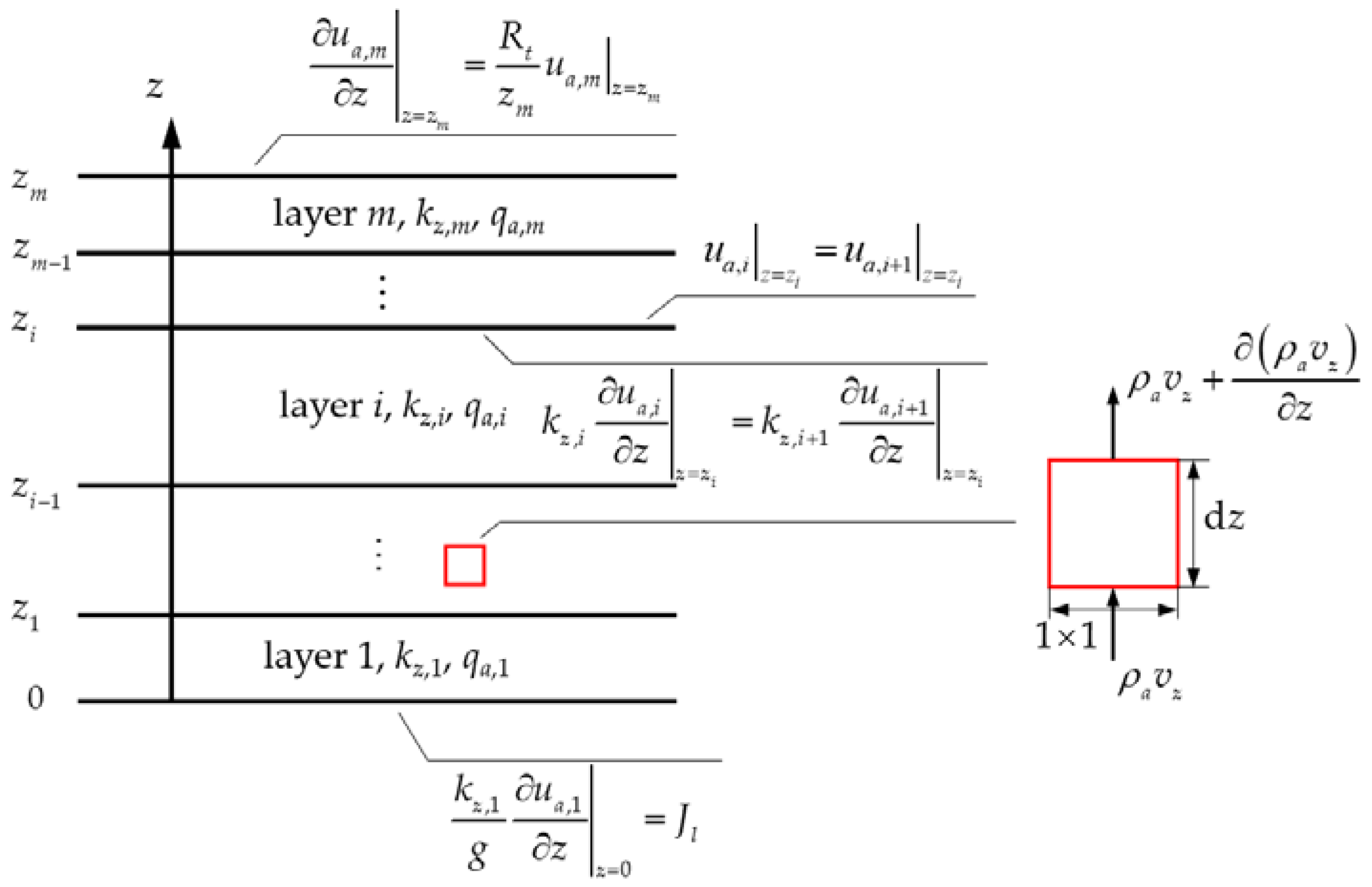
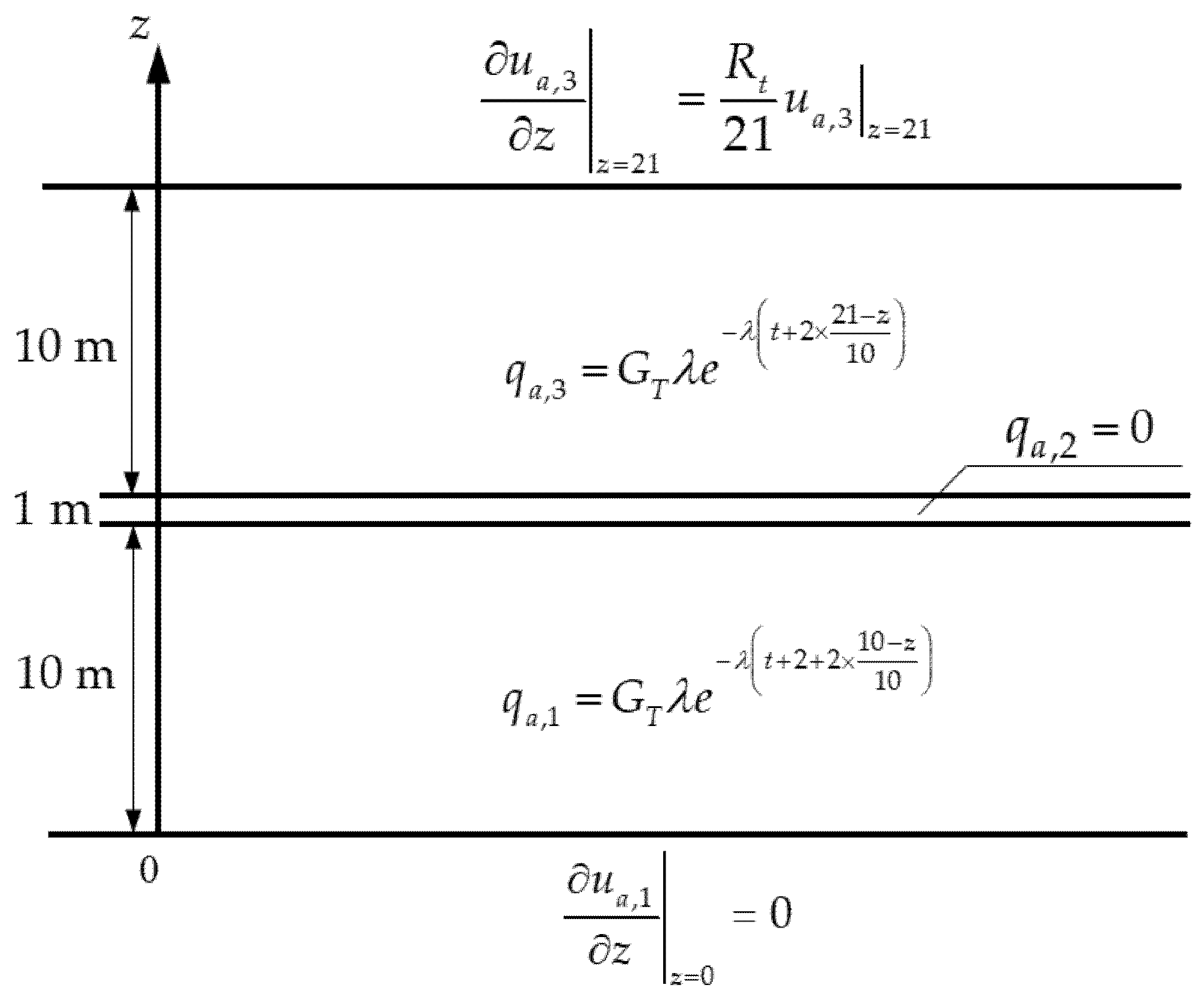
2. Model Development

The assumptions made to derive the mathematical formulation are:

(1)

The landfill gas was assumed to be an equimolar mixture of CH₄ and CO₂ and considered to behave as an ideal gas [23];

(2)

Darcy’s law was applied to the gas flow, and gas diffusion was not considered [23];

(3)

No external load was applied on the landfill, and the vertical stress with respect to the change of time was equal to zero [26];

(4)

The gas flow rate was much greater than the liquid flow rate in the landfill, and the influence of the pore liquid pressure on the gas pressure was neglected [26].

The vertical flow of gas in landfills, as illustrated in Figure 1, was considered. The mass balance equation for a gas in a unit cell of MSW is

$$\frac{1}{V_0}\frac{\partial M_a}{\partial t}=-\frac{\partial \left({\rho }_a{v}_z\right)}{\partial z}+q_a$$

(1)

where V₀ is the volume of the unit cell (m³); M_a is the gas mass in the unit cell (kg); ρ_a is the gas density (kg∙m⁻³); v_z is the vertical flow velocity of the gas (m∙s⁻¹); q_a is the gas generation rate due to the degradation of MSW (kg∙m⁻³∙s⁻¹).

The first-order decomposition rate model is widely used to predict gas generation in landfills [27]:

$$q_a=G_T\lambda e^{-\lambda t}$$

(2)

where G_T is the potential gas generation capacity (kg∙m⁻³); λ is the degradation rate constant (s⁻¹).

To account for the different gas generation rates at different depths in a layer with a linearly depositing rate, Equation (2) can be replaced as follows [23]:

$$q_a=G_T\lambda e^{-\lambda \left(t+\frac{h-z}{h}{t}_f\right)}$$

(3)

where t is the time elapsed since the emplacement of the layer (s); t_f is the time it took to fill the layer (s); h is the thickness of the layer (m).

The gas mass in the unit cell can be expressed as follows:

$$M_a={\rho }_a{V}_a={\rho }_a{V}_{0}n\left(1-S_l\right)$$

(4)

where V_a is the volume of gas in the unit cell (m³); n is the porosity of the unit cell; S_l is the degree of liquid saturation.

Landfill gas is considered an ideal gas in MSW landfills. Therefore,

$${\rho }_a=\frac{{\overline{u}}_a\omega }{RT}$$

(5)

where ω is the average molecular weight of the gas (kg∙mol⁻¹); R is the universal gas constant (J∙mol⁻¹∙K⁻¹); T is the temperature in Kelvin of the gas (K); ${\overline{u}}_a$ is the absolute gas pressure (Pa), which is expressed as

$${\overline{u}}_a=u_a+u_{atm}$$

(6)

where u_a is the excess gas pressure (Pa); u_atm is the atmospheric pressure (101.3 kPa).

Based on Darcy’s law, the vertical flow velocity of the gas can be written as

$$v_z=-\frac{k_z}{{\rho }_{a}g}\frac{\partial u_a}{\partial z}$$

(7)

where k_z is the vertical gas permeability coefficient (m∙s⁻¹); g is the gravitational acceleration (m∙s⁻²).

Substituting Equations (4)–(7) into Equation (1) yields

$$\frac{1}{V_0}\frac{\partial V_a}{\partial t}=\frac{RT{k}_z}{{\overline{u}}_a\omega g}\frac{{\partial }^2{u}_a}{\partial z^2}-\frac{n\left(1-S_l\right)}{{\overline{u}}_a}\frac{\partial u_a}{\partial t}+\frac{RT}{{\overline{u}}_a\omega }{q}_a$$

(8)

According to Boyle’s law,

$$V_{0}n\left(1-S_l\right){\overline{u}}_a=V_0{n}_0\left(1-S_{l0}\right){\overline{u}}_0$$

(9)

where ${\overline{u}}_0$ is the initial absolute gas pressure (Pa); n₀ is the initial porosity of the unit cell; S_l0 is the initial degree of liquid saturation.

The variation of the excess gas pressure in a landfill with respect to u_atm can normally be neglected; ${\overline{u}}_a$ is assumed to be constant. Therefore,

$$n\left(1-S_l\right)=n_0\left(1-S_{l0}\right)$$

(10)

The change rate of the gas volume in a unit volume of MSW can be obtained on the basis of the unsaturated soil gas phase constitutive equation [28], that is

$$\frac{1}{V_0}\frac{\partial V_a}{\partial t}=m_3^a\frac{\partial u_a}{\partial t}$$

(11)

where

$$m_3^a=m_2^a-m_1^a$$

(12)

In Equation (12), $m_1^a$ is the coefficient of the change in gas volume corresponding to the main stress in the lateral confined condition (Pa⁻¹); $m_2^a$ is the coefficient of the change in gas volume corresponding to the suction in the lateral confined condition (Pa⁻¹).

Incorporating Equation (11) into Equation (8) gives

$$\frac{\partial u_a}{\partial t}=\alpha \frac{k_z}{g}\frac{{\partial }^2{u}_a}{\partial z^2}+\alpha q_a$$

(13)

where

$$\alpha =-\frac{RT}{\omega \left[m_3^a{\overline{u}}_0-n_0\left(1-S_{l0}\right)\right]}$$

(14)

A landfill consisting of a finite multilayer is shown in Figure 1. z_i and z_i−1 are the upper depth and lower depth of the ith layer; z_m is the upper depth of the entire landfill.

According to Equations (13) and (14), the governing equation of a vertical gas flow in the ith layer is

$$\frac{\partial u_{a,i}}{\partial t}={\alpha }_i\frac{k_{z,i}}{g}\frac{{\partial }^2{u}_{a,i}}{\partial z^2}+{\alpha }_i{q}_{a,i}, z_{i-1}\le z\le z_i, i=1,2,\dots ,m$$

(15)

where

$${\alpha }_i=-\frac{R{T}_i}{\omega \left[m_{3,i}^a{\overline{u}}_{0,i}-n_{0,i}\left(1-S_{l0,i}\right)\right]}$$

(16)

where u_a,i is the excess gas pressure in the ith layer (Pa); k_z,i is the vertical gas permeability coefficient of the ith layer (m∙s⁻¹); q_a,i is the gas generation in ith layer (kg∙m⁻³∙s⁻¹); T_i is the temperature in Kelvin of the ith layer (K); $m_{3,i}^a=m_{2,i}^a-m_{1,i}^a$; $m_{1,i}^a$ is the gas volume variation coefficient due to the net normal stress under the lateral confined condition in the ith layer (Pa⁻¹); $m_{2,i}^a$ is the gas volume variation coefficient due to matric suction under the lateral confined condition in the ith layer (Pa⁻¹); n_0,i is the initial porosity of the ith layer; S_l0,i is the degree of liquid saturation in the ith layer; ${\overline{u}}_{0,i}$ is the initial absolute gas pressure in the ith layer (Pa).

The boundary conditions are dependent on the operating scenarios of the landfills. The following operating scenarios were considered.

When a low-permeable cover is applied at the top surface of landfill, the boundary condition on the top surface of the landfill is [19]

$${\frac{\partial u_{a,m}}{\partial z}|}_{z=z_m}=\frac{R_t}{z_m}{u_{a,m}|}_{z=z_m}$$

(17)

where R_t is the dimensionless property, as follows

$$R_t=\frac{k_{z,c}{z}_m}{k_{z,m}{h}_c}$$

(18)

In Equation (18), h_c is thickness of the cover (m); k_z,c is the vertical gas permeability coefficient for the top surface (m∙s⁻¹). R_t is dimensionless and reflects the drainage efficiency at the top surface of the gas. The larger the value of R_t, the greater the drainage efficiency, that is, the smaller the hindrance effect on the top surface. When R_t is equal to zero, the boundary is absolutely impermeable to the gas, while when the R_t approaches infinity, the boundary is fully permeable to the gas.

If a fixed gas flux is specified at the bottom, the boundary condition on the bottom surface of the landfill is [8]

$$\frac{k_{z,1}}{g}{\frac{\partial u_{a,1}}{\partial z}|}_{z=0}=J_l$$

(19)

where J_l is the gas flux rate applied at the base (kg∙m⁻²∙s⁻¹). When the bottom surface is absolutely impermeable to the gas, J_l = 0.

The continuity conditions of the adjacent two layers are

$${u_{a,i}|}_{z=z_i}={u_{a,i+1}|}_{z=z_i}, {k_{z,i}\frac{\partial u_{a,i}}{\partial z}|}_{z=z_i}=k_{z,i+1}{\frac{\partial u_{a,i+1}}{\partial z}|}_{z=z_i}, i=1,2,\dots ,m-1$$

(20)

In the transient model, the initial conditions can be expressed as

$${u_{a,i}|}_{t=0}=u_{0,i}, i=1,2,\dots ,m$$

(21)

where u_0,i is the initial excess gas pressure in the ith layer (Pa).

3. Transient Analytical Solution and Application

3.1. Transient Analytical Solution

The superposition method and orthogonal expansion technique were used to obtain the analytical solution of the transient model (see Appendix A). The solution of the excess gas pressure in the ith layer is expressed as

$$\begin{array}{l}{u}_i\left(z,t\right)=a_{i}z+b_i+\\ {\displaystyle \sum _{j=1}^{\infty }\left[c_{i,j}\sin \left({\beta }_{i,j}z\right)+d_{i,j}\cos \left({\beta }_{i,j}z\right)\right]\left[{\displaystyle {\int }_0^t{e}^{-{\alpha }_i\frac{k_{z,i}}{g}{\beta }_{i,j}^2\left(t-\tau \right)}{T}_{q,j}\left(\tau \right)d\tau }+{\phi }_j{e}^{-{\alpha }_i\frac{k_{z,i}}{g}{\beta }_{i,j}^{2}t}\right]}\end{array}$$

(22)

where

$$\begin{array}{l}{a}_1=\frac{J_{l}g}{k_{z,1}}, b_1=\left(\frac{k_{z,1}{h}_m}{R_t{k}_{z,m}}-\frac{k_{z,1}{z}_m}{k_{z,m}}\right)a_1-{\displaystyle \sum _{q=1}^i\left(\frac{k_{z,1}}{k_{z,q}}-\frac{k_{z,1}}{k_{z,q+1}}\right)z_q}{a}_1\\ a_{i+1}=\frac{k_{z,1}}{k_{z,i+1}}{a}_1, b_{i+1}=b_1+{\displaystyle \sum _{q=1}^i\left(\frac{k_{z,1}}{k_{z,q}}-\frac{k_{z,1}}{k_{z,q+1}}\right)z_q}{a}_1, i=1,2,\dots ,m-1\end{array}$$

(23)

$$c_{1,j}=0, d_{1,j}=1$$

(24)

The recursive relationship between c_i,j, d_i,j and c_i+1,j, d_i+1,j (i = 1, 2,…, m−1) are

$$\left[\begin{array}{l}{c}_{i+1,j}\\ d_{i+1,j}\end{array}\right]=\left[\begin{array}{cc}{F}_{i,j}{F}_{i+1,j}+{\chi }_{i,j}{F}_{i,j}{G}_{i+1,j}& G_{i,j}{F}_{i+1,j}-{\chi }_{i,j}{F}_{i,j}{G}_{i+1,j}\\ F_{i,j}{G}_{i+1,j}-{\chi }_{i,j}{F}_{i,j}{F}_{i+1,j}& G_{i,j}{G}_{i+1,j}+{\chi }_{i,j}{F}_{i+1,j}{G}_{i+1,j}\end{array}\right]\left[\begin{array}{l}{c}_{i,j}\\ d_{i,j}\end{array}\right]$$

(25)

where

$${\chi }_{i,j}=\frac{k_{z,i}{\beta }_{i,j}}{k_{z,i+1}{\beta }_{i+1,j}}, F_{i,j}=\sin \left({\beta }_{i,j}{z}_i\right), G_{i,j}=\cos \left({\beta }_{i,j}{z}_i\right)$$

(26)

$${\beta }_{i,j}=\sqrt{\frac{{\alpha }_m{k}_{z,m}}{{\alpha }_i{k}_{z,i}}}{\beta }_{m,j}$$

(27)

β_m,j indicates the roots of the following transcendental equation

$$S_{m-1,j}\left[\begin{array}{c}0\\ 1\end{array}\right]{\left[\begin{array}{c}{R}_t\sin \left({\beta }_{m,j}{z}_m\right)-z_m\cos \left({\beta }_{m,j}{z}_m\right)\\ R_t\sin \left({\beta }_{m,j}{z}_m\right)+z_m\cos \left({\beta }_{m,j}{z}_m\right)\end{array}\right]}^T=0$$

(28)

where

$$S_{m-1,j}={\displaystyle \prod _{i=1}^{m-1}\left[\begin{array}{cc}{F}_{i,j}{F}_{i+1,j}+{\chi }_{i,j}{F}_{i,j}{G}_{i+1,j}& G_{i,j}{F}_{i+1,j}-{\chi }_{i,j}{F}_{i,j}{G}_{i+1,j}\\ F_{i,j}{G}_{i+1,j}-{\chi }_{i,j}{F}_{i,j}{F}_{i+1,j}& G_{i,j}{G}_{i+1,j}+{\chi }_{i,j}{F}_{i+1,j}{G}_{i+1,j}\end{array}\right]}$$

(29)

In Equation (22),

$$T_{q,j}\left(t\right)=\left(\frac{1}{\psi }\right){\displaystyle \sum _{i=1}^m{\displaystyle {\int }_{z_{i-1}}^{z_i}\left[c_{i,j}\sin \left({\beta }_{i,j}z\right)+d_{i,j}\cos \left({\beta }_{i,j}z\right)\right]{\alpha }_i{q}_{a,i}\left(\frac{1}{{\alpha }_i}\right)dz}}$$

(30)

$${\phi }_j=\left(\frac{1}{\psi }\right){\displaystyle \sum _{i=1}^m{\displaystyle {\int }_{z_{i-1}}^{z_i}\left[c_{i,j}\sin \left({\beta }_{i,j}z\right)+d_{i,j}\cos \left({\beta }_{i,j}z\right)\right]\left(u_{0,i}-a_{i}z-b_i\right)\left(\frac{1}{{\alpha }_i}\right)}dz}$$

(31)

where

$$\psi ={\displaystyle \sum _{i=1}^m{\displaystyle {\int }_{z_{i-1}}^{z_i}{\left[c_{i,j}\sin \left({\beta }_{i,j}z\right)+d_{i,j}\cos \left({\beta }_{i,j}z\right)\right]}^2\left(\frac{1}{{\alpha }_i}\right)dz}}$$

(32)

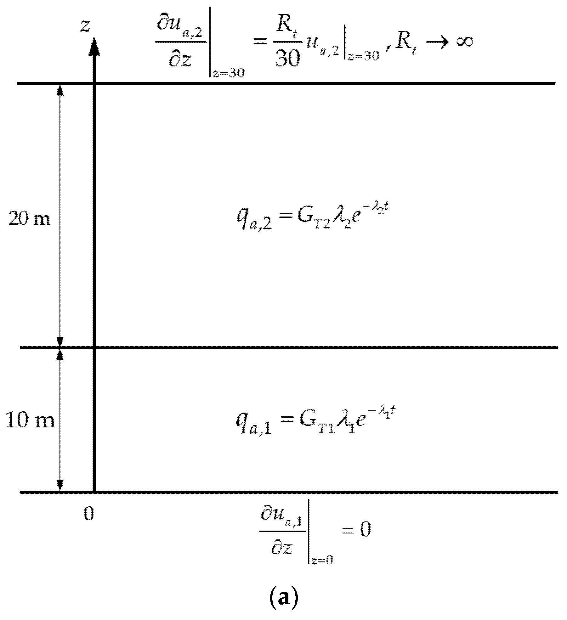
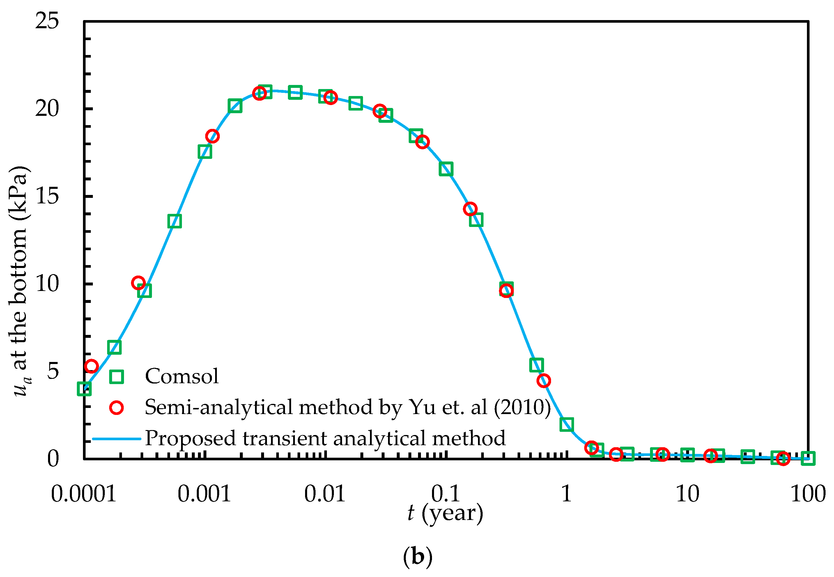
3.2. Verification of the Transient Analytical Solution

Yu et al. [19] proposed a vertical gas flow model for a landfill with layered MSW. The excess gas pressure of a landfill with two-layered MSWs was calculated by the semi-analytical solution in Yu et al.’s study. The calculation example of the two-layered landfill was adopted here. A schematic diagram of the landfill is shown in Figure 2a. The initial excess gas pressure was assumed to be 0. The parameter $m_3^a$ in this study was approximately set to −1/E₀ in $m_k^a$ of Yu et al.’s study. The other parameters were the same as those in Yu et al.’s study. The values of the parameters are listed in

Table 1. Model parameters used by Yu et al. [19].

Parameters	Value
kz,1 (m∙s−1)	5 × 10−7
kz,2 (m∙s−1)	1.2 × 10−6
n0,1	0.5
n0,2	0.5
Sl0,1	0
Sl0,2	0
u0,1 (Pa)	0
u0,2 (Pa)	0
T1 (K)	310
T2 (K)	310
$m_{3,1}^a$ (kPa−1)	−5 × 10−20
$m_{3,2}^a$ (kPa−1)	−2 × 10−4
ω (kg∙mol−1)	0.03
R (J∙mol−1∙K−1)	8.314
GT1 (kg∙m−3)	100
GT2 (kg∙m−3)	220
λ1 (year−1)	2.523
λ2 (year−1)	0.02523

. COMSOL Multiphysics is a widely used software based on the finite element method [29]. COMSOL simulation was used to verify the proposed transient analytical solution. The gas pressure at the bottom of the landfill obtained by the proposed transient analytical method and COMSOL is shown in Figure 2b. The relative error between the two methods was less than 0.5%. The analytical solution agreed with the numerical solution very well. Therefore, the correctness of the transient analytical solution was proved.

The proposed transient analytical method and Yu et al.’s semi-analytical method were compared. The gas pressure at the bottom of the landfill determined by the two methods is presented in Figure 2b. The results obtained by these two methods were in good agreement. However, the mechanical compression of the solid skeleton was coupled with gas pressure using the K-H viscoelastic model in Yu et al.’s study, while the unsaturated soils theory of Fredlund and Rahardjo [28] was adopted in this study. Thus, the parameter α was different in the two studies, which resulted in a slight difference in the gas pressure at the early times.

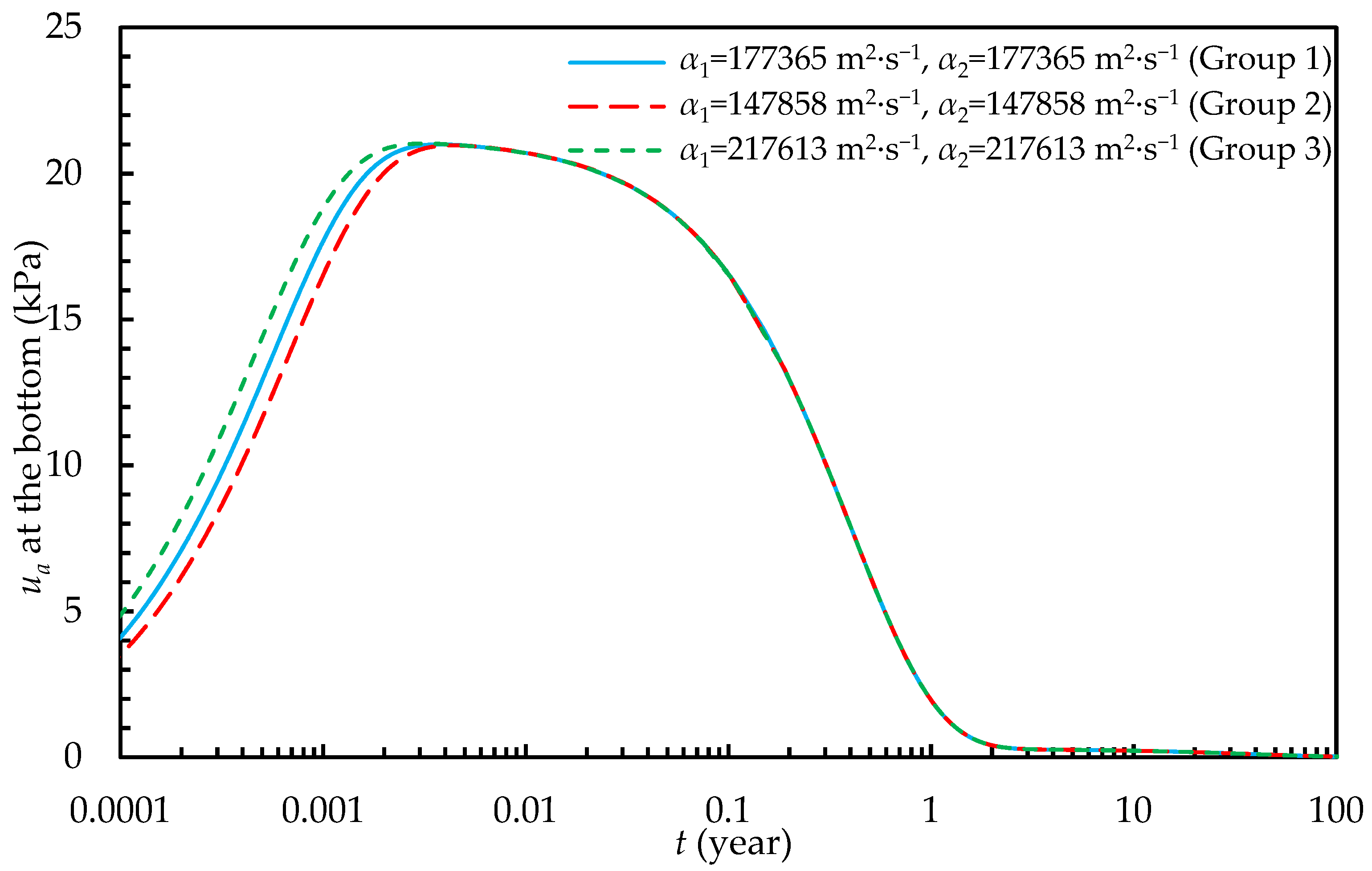
3.3. Application of the Transient Analytical Solution

The effect of the parameter α on the gas pressure was also investigated by the transient analytical solution. Three groups of the parameters S_l0,1, S_l0,2, T₁, T₂, $m_{3,1}^a$ and $m_{3,2}^a$ are shown in

Table 2. Parameters groups.

Parameter	Group 1	Group 2	Group 3
α1 (m2∙s−1)	177,365	147,858	217,613
α2 (m2∙s−1)	177,365	147,858	217,613
Sl0,1	0	0	0.2
Sl0,2	0	0	0.2
T1 (K)	310	310	330
T2 (K)	310	310	330
$m_{3,1}^a$ (kPa−1)	0	−8 × 10−4	−2 × 10−4
$m_{3,2}^a$ (kPa−1)	0	−8 × 10−4	−2 × 10−4

and resulted in different values of the parameters α₁ and α₂. The values of other parameters were the same as those in Table 1. It can be seen in Figure 3 that the effects of the parameter α are only relevant for the early response.

On the other hand, Equation (15) can be rewritten as follows

$$\frac{1}{{\alpha }_i}\frac{\partial u_{a,i}}{\partial t}=\frac{k_{z,i}}{g}\frac{{\partial }^2{u}_{a,i}}{\partial z^2}+q_{a,i}, z_{i-1}\le z\le z_i, i=1,2,\dots ,m$$

(33)

It can be seen from Table 2 that the values of the parameter α_i were much larger than 1. Thus, the left side of Equation (15) approximated 0. This means that the time scale of the gas flow dynamics within the landfill could be neglected, and the gas flow could be approximated to a quasi-steady-state process, as follows

$$\frac{k_{z,i}}{g}\frac{{\partial }^2{u}_{a,i}}{\partial z^2}+q_{a,i}=0, z_{i-1}\le z\le z_i, i=1,2,\dots ,m$$

(34)

4. Quasi-Steady-State Analytical Solution and Validation

4.1. Quasi-Steady-State Analytical Solution

Solving the ordinary differential Equation (34) by the direct integration method, the quasi-steady-state analytical solution can be obtained as follows

$$u_{a,i}\left(z,t\right)=-\frac{g}{k_{z,i}}{Q}_{2,i}+r_{i}z+s_i, z_{i-1}\le z\le z_i, i=1,2,\dots ,m$$

(35)

where

$$Q_{2,i}={\displaystyle \int Q_{1,i}\mathrm{d}z}, Q_{1,i}={\displaystyle \int q_{a,i}\mathrm{d}z}$$

(36)

Substituting Equation (35) into the boundary conditions of Equations (17) and (19) yields

$$-\frac{g}{k_{z,m}}{Q_{1,m}|}_{z=z_m}+r_m=\frac{R_t}{z_m}\left[-\frac{g}{k_{z,m}}{Q_{2,m}|}_{z=z_m}+r_m{z}_m+s_m\right]$$

(37)

$$-\frac{g}{k_{z,1}}{Q_{1,1}|}_{z=0}+r_1=\frac{J_{l}g}{k_{z,1}}$$

(38)

Substituting Equation (35) into the continuity conditions Equation (20) yields

$$-\frac{g}{k_{z,i}}{Q_{2,i}|}_{z=z_i}+r_i{z}_i+s_i=-\frac{g}{k_{z,i}}{Q_{2,i+1}|}_{z=z_i}+r_{i+1}{z}_i+s_{i+1}$$

(39)

$$-g{Q_{1,i}|}_{z=z_i}+k_{z,i}{r}_i=-g{Q_{1,i+1}|}_{z=z_i}+k_{z,i+1}{r}_{i+1}$$

(40)

Using Equations (37)–(40), r_i and s_i can be determined in the form of matrices, as follows

$$C=D^{-1}E$$

(41)

where C, D, E are a 2n × 1, 2n × 2n, 2n × 1 matrix, as follows

$$C={\left[\begin{array}{cccc}\begin{array}{cc}{r}_m& s_m\end{array}& \begin{array}{cc}\dots & \begin{array}{cc}{r}_i& s_i\end{array}\end{array}& \dots & \begin{array}{cc}{r}_1& s_1\end{array}\end{array}\right]}^T$$

(42)

$$D=\left[\begin{array}{ccccc}{D}_{up}& \dots & 0& \dots & 0\\ D_{n-1}& \dots & 0& \dots & 0\\ \dots & \dots & \dots & \dots & \dots \\ 0& \dots & D_i& \dots & 0\\ \dots & \dots & \dots & \dots & \dots \\ 0& \dots & 0& \dots & D_1\\ 0& \dots & 0& \dots & D_{lo}\end{array}\right]$$

(43)

$$E={\left[\begin{array}{ccccccc}{E}_{up}& E_{n-1}& \dots & E_i& \dots & E_1& E_{lo}\end{array}\right]}^T$$

(44)

In Equations (43) and (44), 0 indicates a zero matrix,

$$D_i=\left[\begin{array}{cccc}{z}_i& 1& -z_i& -1\\ k_{z,i}& 0& -k_{z,i+1}& 0\end{array}\right]$$

(45)

$$D_{up}=\left[\begin{array}{cccc}1-\frac{R_t}{z_m}{z}_m& -\frac{R_t}{z_m}& 0& 0\end{array}\right]$$

(46)

$$D_{lo}=\left[\begin{array}{cccc}0& 0& 1& 0\end{array}\right]$$

(47)

$$E_i=\left[\begin{array}{cc}\frac{g}{k_{z,i}}{Q_{2,i}|}_{z=z_i}-\frac{g}{k_{z,i+1}}{Q_{2,i+1}|}_{z=z_i}& g{Q_{1,i}|}_{z=z_i}-g{Q_{1,i+1}|}_{z=z_i}\end{array}\right]$$

(48)

$$E_{up}=\left[-\frac{g}{k_{z,m}}\frac{R_t}{h_m}{Q_{2,m}|}_{z=z_m}+\frac{g}{k_{z,m}}{Q_{1,m}|}_{z=z_m}\right]$$

(49)

$${{\rm E}}_{lo}=\left[\frac{J_{l}g}{k_{z,1}}+\frac{g}{k_{z,1}}{Q_{1,1}|}_{z=0}\right]$$

(50)

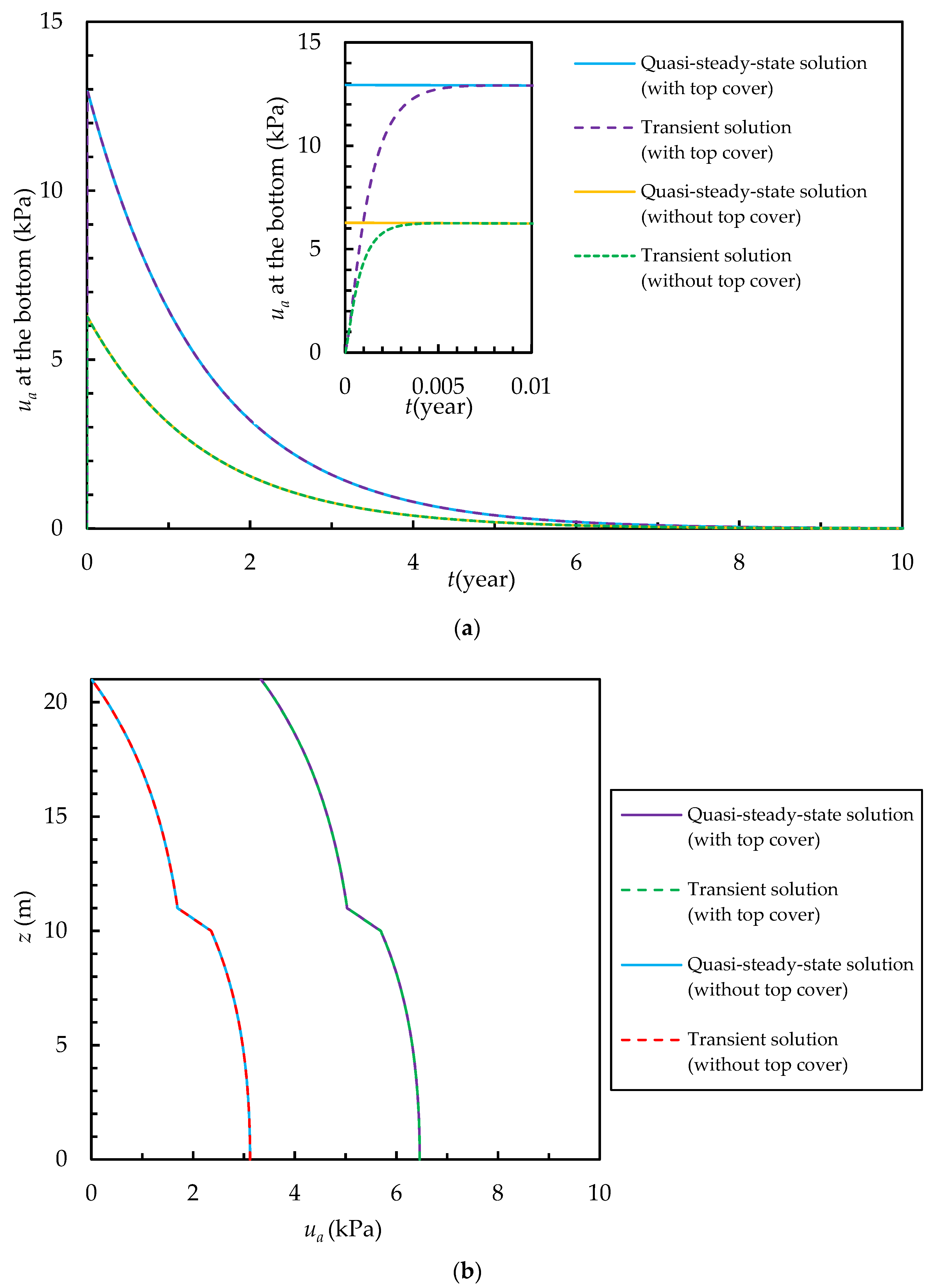
4.2. Comparison of the Quasi-Steady-State and Transient Solutions

A new calculation example was proposed, in which the temporal and spatial variability of the gas generation rate was considered. A landfill containing two layers of MSW and an intermediate cover was considered. The landfill is illustrated in Figure 4. The height of each MSW layer was assumed to be 10 m, and the filling of each MSW layer took 2 years. The filling time of the intermediate cover was much shorter than the time required to form an MSW layer and was not considered in the study. A high mass fraction of food waste was shown to result in a high liquid saturation of wastes in China [30,31]. The values of porosity n and liquid saturation S_l were selected according to their common value range for landfills in China. The gas permeability of MSW corresponding to a specific porosity n and liquid saturation S_l was based on the experimental result by Shi et al. [32]. Two kinds of boundary conditions on the top surface of the landfill were considered, i.e., with or without the top cover. When there is no top cover, R_t approaches infinity. The thickness and vertical gas permeability of the top cover are shown in

Table 3. Model parameters.

Parameters	Value
kz1 (m∙s−1) [32]	1 × 10−7
kz,2 (m∙s−1) [21]	6 × 10−8
kz,3 (m∙s−1) [32]	3 × 10−7
kc (m∙s−1) [19]	3 × 10−8
hc (m) [19]	1
n0,1 [30,31]	0.667
n0,2 [31,32]	0.333
n0,3 [30,31]	0.737
Sl0,1 [30,31]	0.8
Sl0,2 [30,31]	0.78
Sl0,3 [30,31]	0.75
T1 (K) [19]	310
T2 (K) [19]	310
T3 (K) [19]	310
$m_{3,1}^a$ (kPa−1) [28]	−6 × 10−4
$m_{3,2}^a$ (kPa−1) [28]	−6 × 10−4
$m_{3,3}^a$ (kPa−1) [28]	−6 × 10−4
ω (kg∙mol−1) [8,23]	0.03
R (J∙mol−1∙K−1) [8,23]	8.314
GT (kg∙m−3) [21]	138
λ (year−1) [21]	0.7

. The initial excess gas pressure was assumed to be 0 in the following analysis.

Equation (3) was adopted to describe the gas generation in the two MSW layers. The gas generation in the first MSW layer was as follows

$$q_{a,1}=G_T\lambda e^{-\lambda \left(t+2\times \frac{10-z}{10}\right)}$$

(51)

The gas generation in the second MSW layer was as follows

$$q_{a,3}=G_T\lambda e^{-\lambda \left(t+2+2\times \frac{21-z}{10}\right)}$$

(52)

All parameters are listed in Table 3. They were within the typical ranges suggested from previous publications.

The evolution of gas pressure with time at the bottom of the landfill was calculated by the transient analytical solution and quasi-steady-state analytical solution, as shown in Figure 5a. The evolution of the gas pressure with depth at t = 1 year was also calculated by the transient analytical solution and quasi-steady-state analytical solution, as shown in Figure 5b. The relative error of the gas pressures (t > 0.006 year) determined using the two methods was less than 0.5%. The results obtained from the transient analytical solution and quasi-steady-state analytical solution were in good agreement. There was only a slight difference in the gas pressure at an early time (<0.006 year). This demonstrates that the quasi-steady-state solution can reliably estimate the gas pressure in landfills.

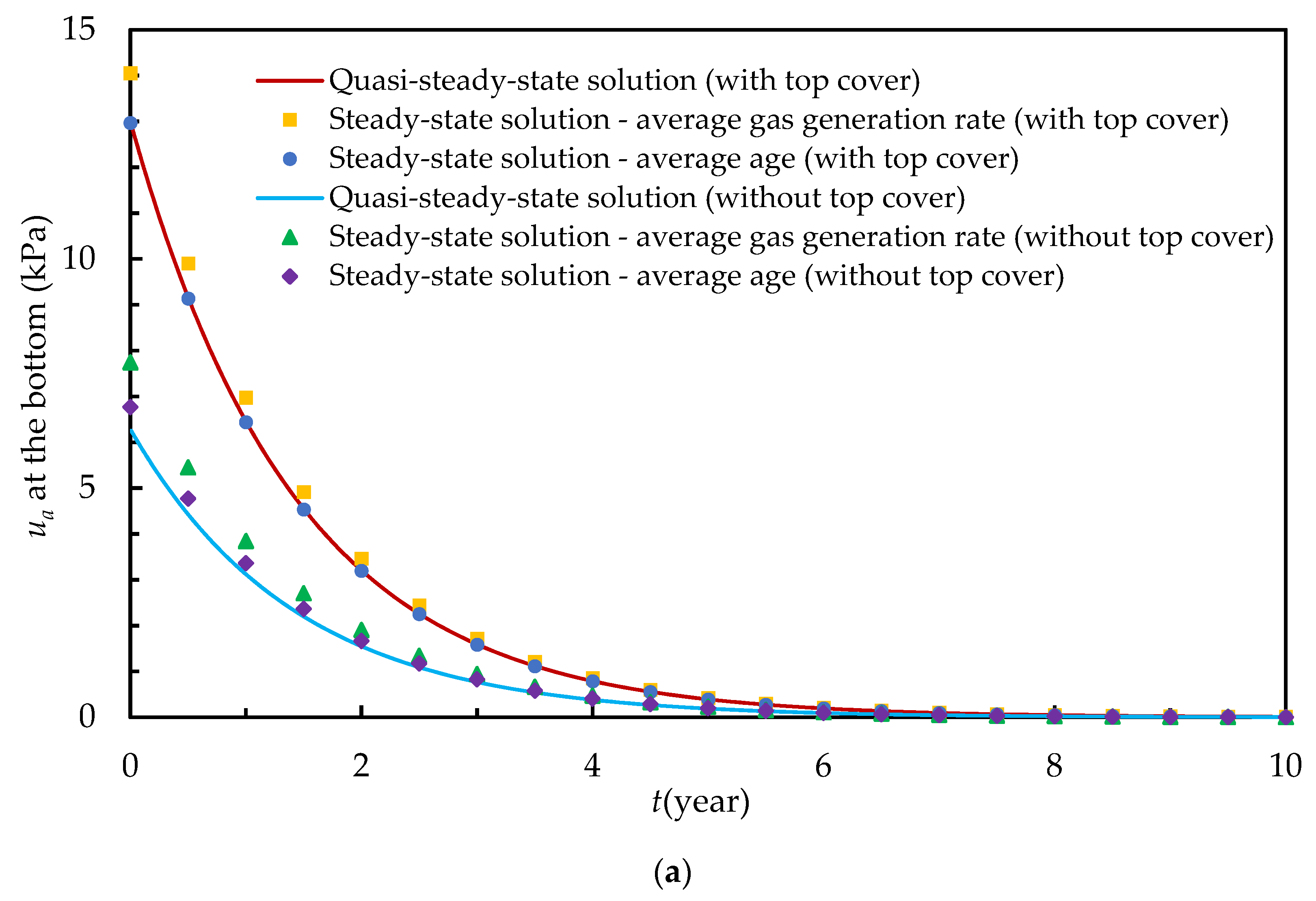
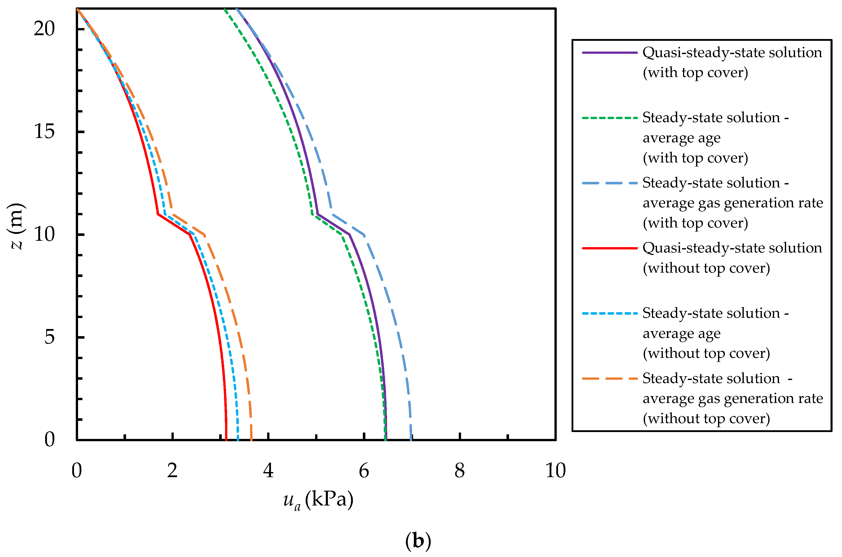
4.3. Comparison of the Quasi-Steady-State and Steady-State Solutions

When the gas generation rate q_a,i in Equation (34) is a constant, the quasi-steady-state governing equations become the steady-state governing equations. Li et al. [9] proposed a steady-state analytical model for the vertical gas flow in a landfill with layered MSW. The values of the gas generation rate in each layer at a certain time used in the steady-state model are the average values of the gas generation rate in the layer or the gas generation rate corresponding to the average age of each layer.

The average value of gas generation ${\overline{q}}_{a,i}$ was calculated as follows

$${\overline{q}}_{a,i}=\frac{1}{z_i-z_{i-1}}{\displaystyle {\int }_{z_{i-1}}^{z_i}{q}_{a,i}}\mathrm{d}z$$

(53)

The landfill in Section 4.2 was considered. The gas pressure was calculated by the proposed quasi-steady-state solution and the steady-state solution by Li et al. [9]. As shown in Figure 6, the steady-state model resulted in an error in the estimation of gas pressure. For instance, the gas pressure at the bottom of the landfill without a top cover obtained by the steady-state solution using the average gas generation rate corresponding to the average age was 8.7% greater than that obtained by the quasi-steady-state solution, at t = 0.5 year. The gas pressure at the bottom of the landfill with a top cover obtained by the steady-state solution using the average gas generation rate was 8% greater than that obtained by the quasi-steady-state solution, at t = 1 year. Thus, it is necessary to consider the variation of the gas generation rate in the depth of a landfill in relation to the fill age when predicting the gas pressure in MSW landfills.

5. Conclusions

In this paper, a one-dimensional analytical model was proposed to simulate the vertical gas flow in a landfill with layered MSW. Temporal and spatial variations of the gas generation rate in the MSW were considered. A transient analytical solution was obtained by the superposition method and the orthogonal expansion technique. A quasi-steady-state analytical solution was also obtained by the direct integration method. Several conclusions can be drawn on the basis of the adopted solution, as shown below:

(1)

According to the results of the parameter analysis by the transient analytical solution, the vertical gas flow in landfills can be simplified to a quasi-steady-state flow.

(2)

The gas pressure values obtained by the transient and quasi-steady-state analytical solutions were in good agreement. There was only a slight difference in the gas pressure at the early times. The quasi-steady-state solution can reliably estimate the gas pressure in landfills.

(3)

Using the average gas generation rate or the gas generation rate corresponding to the average age of the MSW layer in the steady-state model resulted in an error in the estimation of gas pressure in landfills.

(4)

The axisymmetric transient and quasi-steady-state analytical models for the gas flow around a vertical well in a layered landfill can be proposed by extension of the results of this paper.

References

1. Parameswaran, T.G.; Sivakumar Babu, G.L. Design of gas collection systems: Issues and challenges. Waste Manag. Res. 2022, 0734242X221086949. [Google Scholar] [CrossRef] [PubMed]
2. Duan, Z.; Scheutz, C.; Kjeldsen, P. Trace gas emissions from municipal solid waste landfills: A review. Waste Manag. 2021, 119, 39–62. [Google Scholar] [CrossRef] [PubMed]
3. Paraskaki, I.; Lazaridis, M. Quantification of landfill emissions to air: A case study of the Ano Liosia landfill site in the greater Athens area. Waste Manag. Res. 2005, 23, 199–208. [Google Scholar] [CrossRef] [PubMed]
4. Tian, H.; Gao, J.; Hao, J.; Lu, L.; Zhu, C.; Qiu, P. Atmospheric pollution problems and control proposals associated with solid waste management in China: A review. J. Hazard. Mater. 2013, 252, 142–154. [Google Scholar] [CrossRef]
5. Liu, Y.; Lu, W.; Dastyar, W.; Liu, Y.; Guo, H.; Fu, X.; Li, H.; Meng, R.; Zhao, M.; Wang, H. Fugitive halocarbon emissions from working face of municipal solid waste landfills in China. Waste Manag. 2017, 70, 149–157. [Google Scholar] [CrossRef]
6. Ke, H.; Hu, J.; Chen, Y.M.; Lan, J.W.; Zhan, L.T.; Meng, M.; Yang, Y.Q.; Li, Y.C. Foam-induced high gas pressures in wet municipal solid waste landfills. Géotechnique 2021, 72, 860–871. [Google Scholar] [CrossRef]
7. Shu, S.; Li, Y.; Sun, Z.; Shi, J. Effect of gas pressure on municipal solid waste landfill slope stability. Waste Manag. Res. 2022, 40, 323–330. [Google Scholar] [CrossRef]
8. Townsend, T.G.; Wise, W.R.; Jain, P. One-dimensional gas flow model for horizontal gas collection systems at municipal solid waste landfills. J. Environ. Eng. 2005, 131, 1716–1723. [Google Scholar] [CrossRef]
9. Li, Y.C.; Zheng, J.; Chen, Y.M.; Guo, R.Y. One-dimensional transient analytical solution for gas pressure in municipal solid waste landfills. J. Environ. Eng. 2013, 139, 1441–1445. [Google Scholar] [CrossRef]
10. Zeng, G. Study on landfill gas migration in landfilled municipal solid waste based on gas-solid coupling model. Environ. Prog. Sustain. 2020, 39, e13352. [Google Scholar] [CrossRef]
11. Feng, S.J.; Wu, S.J.; Zheng, Q.T. Design method of a modified layered aerobic waste landfill divided by coarse material. Environ. Sci. Pollut. Res. 2021, 28, 2182–2197. [Google Scholar] [CrossRef] [PubMed]
12. Zhang, T.; Shi, J.; Qian, X.; Ai, Y. Temperature monitoring during a water-injection test using a vertical well in a newly filled MSW layer of a landfill. Waste Manag. Res. 2019, 37, 530–541. [Google Scholar] [CrossRef] [PubMed]
13. Jain, P.; Powell, J.; Townsend, T.G.; Reinhart, D.R. Air permeability of waste in a municipal solid waste landfill. J. Environ. Eng. 2012, 131, 1565–1573. [Google Scholar] [CrossRef]
14. Zhang, W.; Lin, M. Evaluating the dual porosity of landfilled municipal solid waste. Environ. Sci. Pollut. Res. 2019, 26, 12080–12088. [Google Scholar] [CrossRef] [PubMed]
15. Jung, Y.J.; Imhoff, P.T.; Augenstein, D.C.; Yazdani, R. Influence of high-permeability layers for enhancing landfill gas capture and reducing fugitive methane emissions from landfills. J. Environ. Eng. 2009, 135, 138–146. [Google Scholar] [CrossRef]
16. Hettiarachchi, C.H.; Meegoda, J.N.; Tavantzis, J.; Hettiaratchi, P. Numerical model to predict settlements coupled with landfill gas pressure in bioreactor landfills. J. Hazard. Mater. 2007, 139, 514–522. [Google Scholar] [CrossRef]
17. Zhang, T.; Shi, J.; Wu, X.; Lin, H.; Li, X. Simulation of gas transport in a landfill with layered new and old municipal solid waste. Sci. Rep. 2021, 11, 9436. [Google Scholar] [CrossRef]
18. Xie, H.; Fei, S.; He, H.; Zhang, A.; Ni, J.; Chen, Y. Field investigation and numerical modelling of gas extraction in a heterogeneous landfill with high leachate level. Environ. Sci. Pollut. Res. 2022, 1–17. [Google Scholar] [CrossRef]
19. Yu, L.; Batlle, F.; Carrera, J.; Lloret, A. A coupled model for prediction of settlement and gas flow in MSW landfills. Int. J. Numer. Anal. Meth. Geomech. 2010, 34, 1169–1190. [Google Scholar] [CrossRef]
20. Li, Y.C.; Cleall, P.J.; Ma, X.F.; Zhan, T.L.; Chen, Y.M. Gas pressure model for layered municipal solid waste landfills. J. Environ. Eng. 2012, 138, 752–760. [Google Scholar] [CrossRef]
21. Feng, S.J.; Zheng, Q.T. A two-dimensional gas flow model for layered municipal solid waste landfills. Comput. Geotech. 2015, 63, 135–145. [Google Scholar] [CrossRef]
22. Feng, S.J.; Zheng, Q.T.; Xie, H.J. A gas flow model for layered landfills with vertical extraction wells. Waste Manag. 2017, 66, 103–113. [Google Scholar] [CrossRef] [PubMed]
23. Arigala, S.G.; Tsotsis, T.T.; Webster, I.A.; Yortsos, Y.C. Gas generation, transport, and extraction in landfills. J. Environ. Eng. 1995, 121, 33–44. [Google Scholar] [CrossRef]
24. Amini, H.R.; Reinhart, D.R.; Niskanen, A. Comparison of first-order-decay modeled and actual field measured municipal solid waste landfill methane data. Waste Manag. 2013, 33, 2720–2728. [Google Scholar] [CrossRef]
25. Majdinasab, A.; Zhang, Z.; Yuan, Q. Modelling of landfill gas generation: A review. Rev. Environ. Sci. Bio/Technol. 2017, 16, 361–380. [Google Scholar] [CrossRef]
26. Liu, X.D.; Shi, J.; Qian, X.; Hu, Y.; Peng, G. One-dimensional model for municipal solid waste (MSW) settlement considering coupled mechanical-hydraulic-gaseous effect and concise calculation. Waste Manag. 2011, 31, 2473–2483. [Google Scholar] [CrossRef]
27. SWAMA. Comparison of Models for Predicting Landfill Methane Recovery Publication; The Solid Waste Association of North America (SWANA): San Diego, CA, USA, 1998. [Google Scholar]
28. Fredlund, D.G.; Rahardjo, H. Soil Mechanics for Unsaturated Soils; John Wiley & Sons: Hoboken, NJ, USA, 1993. [Google Scholar]
29. COMSOL. COMSOL Multiphysics v5.5. 2020. [Google Scholar]
30. Xu, X.B.; Zhan, T.L.T.; Chen, Y.M.; Beaven, R.P. Intrinsic and relative permeabilities of shredded municipal solid wastes from the Qizishan landfill, China. Can. Geotech. J. 2014, 51, 1243–1252. [Google Scholar] [CrossRef]
31. Zhang, T.; Shi, J.; Qian, X.; Ai, Y. Temperature and gas pressure monitoring and leachate pumping tests in a newly filled MSW layer of a landfill. Int. J. Environ. Res. 2019, 13, 1–19. [Google Scholar] [CrossRef]
32. Shi, J.; Wu, X.; Ai, Y.; Zhang, Z. Laboratory test investigations on soil water characteristic curve and air permeability of municipal solid waste. Waste Manag. Res. 2018, 36, 463–470. [Google Scholar] [CrossRef]
33. Guerrero, J.S.P.; Pimentel, L.; Skaggs, T.H.; Van Genuchten, M.T. Analytical solution of the advection-diffusion transport equation using a change-of-variable and integral transform technique. Int. J. Heat Mass Transf. 2009, 52, 3297–3304. [Google Scholar] [CrossRef]
Figure 1. Schematic diagram of the vertical gas flow in a landfill with layered MSW (red rectangle represents a unit of MSW).
Mathematics 10 03658 g001
Figure 2. Comparison between the proposed transient analytical method and the numerical and semi-analytical method [19]. (a) Illustration of a two-layered landfill. (b) Comparison of the gas pressure values obtained using the different methods.
Mathematics 10 03658 g002aMathematics 10 03658 g002b
Figure 3. Effect of the parameter α on the gas pressure.
Mathematics 10 03658 g003
Figure 4. Illustration of a landfill containing two layers of MSW and an intermediate cover.
Mathematics 10 03658 g004
Figure 5. Gas pressure calculated by the transient analytical solution and the quasi-steady-state analytical solution. (a) Gas pressure changing with time. (b) Gas pressure changing with depth at t = 1 year.
Mathematics 10 03658 g005
Figure 6. Changes of the gas pressure with time, calculated by the quasi-steady-state analytical solution and the steady-state analytical solution. (a) Gas pressure changing with time. (b) Gas pressure changing with depth at t = 1 year.
Mathematics 10 03658 g006aMathematics 10 03658 g006b