A Family of Hybrid Stochastic Conjugate Gradient Algorithms for Local and Global Minimization Problems

Abstract

This paper contains two main parts, Part I and Part II, which discuss the local and global minimization problems, respectively. In Part I, a fresh conjugate gradient (CG) technique is suggested and then combined with a line-search technique to obtain a globally convergent algorithm. The finite difference approximations approach is used to compute the approximate values of the first derivative of the function f. The convergence analysis of the suggested method is established. The comparisons between the performance of the new CG method and the performance of four other CG methods demonstrate that the proposed CG method is promising and competitive for finding a local optimum point. In Part II, three formulas are designed by which a group of solutions are generated. This set of random formulas is hybridized with the globally convergent CG algorithm to obtain a hybrid stochastic conjugate gradient algorithm denoted by HSSZH. The HSSZH algorithm finds the approximate value of the global solution of a global optimization problem. Five combined stochastic conjugate gradient algorithms are constructed. The performance profiles are used to assess and compare the rendition of the family of hybrid stochastic conjugate gradient algorithms. The comparison results between our proposed HSSZH algorithm and four other hybrid stochastic conjugate gradient techniques demonstrate that the suggested HSSZH method is competitive with, and in all cases superior to, the four algorithms in terms of the efficiency, reliability and effectiveness to find the approximate solution of the global optimization problem that contains a non-convex function.

1. Introduction

The major goal of this paper is to find the local and global minima of a convex and non-convex function. The local and global minimization problems are defined as follows.

Definition 1.

A local minimum ${\mathit{x}}_{\mathit{lo}}\in \mathbb{S}$ of the function f, $f:\mathbb{S}\to \mathbb{R}$ is an input element with $f\left({\mathit{x}}_{\mathit{lo}}\right)\le f\left(\mathit{x}\right)$ for all $\mathit{x}$ neighboring ${\mathit{x}}_{\mathit{lo}}$. If $\mathbb{S}\subseteq {\mathbb{R}}^n$, it is formulated by

$$\forall {\mathit{x}}_{\mathit{lo}}\exists \epsilon >0:f\left({\mathit{x}}_{\mathit{lo}}\right)\le f\left(\mathit{x}\right)\forall \mathit{x}\in \mathbb{S},\parallel \mathit{x}-{\mathit{x}}_{\mathit{lo}}\parallel \le \epsilon .$$

(1)

Definition 2.

The point ${\mathit{x}}_{\mathit{gl}}\in \mathbb{S}$ is called the global minimizer of the function f; $f:\mathbb{S}\to \mathbb{R}$ such that $f\left({\mathit{x}}_{\mathit{gl}}\right)\le f\left(\mathit{x}\right)$ $\forall \mathit{x}\in \mathbb{S}$. When $S\subseteq {\mathbb{R}}^n$, then the problem can be formulated by

$$\underset{\mathit{x}\in \mathbb{S}}{min}f\left(\mathit{x}\right):\mathbb{S}\to \mathbb{R},$$

(2)

In both problems (formulae) $\mathbb{S}\subseteq {\mathbb{R}}^n$ is the range in which we find the global minimizer of $f\left(\mathit{x}\right)$. $f\left(\mathit{x}\right)$ is continuously differentiable.

Global optimization (GO) attempts to find the approximate solution of the objective function are shown in Problem (2).

However, this task can be difficult since the knowledge about f is usually only local. On the other hand, the fastest algorithms (LO) prefer to find a local point since these algorithms are not capable of finding the global solution at each run.

The bottom line is that the core difference between the GO methods and the LO algorithms is as follows: the GO methods focus on solving Problem (2) over the given set, while the task of the LO methods is to solve (1). Consequently, solving Problem (1) is relatively simple by using deterministic (classical) local optimization methods. On the contrary, finding the global optimum of Problem (2) is an NP-hard problem.

Challenging problems arise in different application fields, for example, technical sciences, industrial engineering, economics, networks, chemical engineering, etc. See [1,2,3,4,5,6,7,8,9,10,11].

Recently, many optimization algorithms have been proposed to deal with these problems. The thoughts of those suggested methods rely on the standard of meta-heuristic strategies (random search).

There are different classifications for meta-heuristic methods [12].

Mohamed et al. [7] presented a brief description of these classifications.

In random algorithms, the minimization technique relies partly on probability.

In contrast, in the deterministic algorithms, a guessing scale is not utilized. Hence, deterministic techniques need an exhaustive examination over the research domain of function f to find the approximate solution to Problem (2) at each run. Otherwise, they fail in this task.

Therefore, finding the approximate solution to Problem (2) by using random techniques can be proved by the asymptotic convergence probability. See [13,14,15].

There are many deterministic methods that have been proposed for dealing with the local optimization problems. See, for example, Refs. [16,17,18,19,20].

The most popular deterministic method is the CG method [18]. CG methods are exceedingly utilized to find the local minimizer of Problem (1) [21].

However, the  CG algorithms have a numerical weakness, so their subsequent actions might be low if a little step is created away from the local point. Hence, for solving this issue, a line-search technique is combined with the CG technique to create a globally convergent algorithm [22,23].

Therefore, many conjugant gradient line-search methods are suggested; see, for example, refs. [18,24,25,26,27,28].

The CG method is an efficient and inexpensive technique to deal with Problem (1).

The CG method is an iterative algorithm. Therefore, the candidate solutions are generated by the following recursive formula.

$${\mathit{x}}_{\mathit{k}+\mathbf{1}}={\mathit{x}}_{{}_{\mathit{k}}}+{\alpha }_{{}_k}{\mathit{d}}_{{}_{\mathit{k}}},$$

(3)

where the step size ${\alpha }_{{}_k}>0$, and the directions ${\mathit{d}}_{{}_{\mathit{k}}}$ are created by the following formula:

$${\mathit{d}}_{\mathit{k}+\mathbf{1}}=-{\mathit{g}}_{{}_{\mathit{k}+\mathbf{1}}}+{\beta }_{{}_k}{\mathit{d}}_{{}_{\mathit{k}}},{\mathit{d}}_{{}_{\mathbf{0}}}=-{\mathit{g}}_{{}_{\mathbf{0}}}.$$

(4)

where ${\mathit{g}}_{{}_{\mathit{k}}}$ denotes the gradient vector of the function f at the point ${\mathit{x}}_{{}_{\mathit{k}}}$.

Several versions of the CG methods are suggested. The core difference between those CG algorithms relies on choosing the parameter ${\beta }_{{}_k}$ [18,27,28,29]. The main features of the CG method are as follows: it has low memory requirements, it is strongly local, and it has global convergence properties [30].

Many authors presented several studies to analyze the CG method; see, for example, Refs. [31,32].

In 1964, the authors of [33] applied the CG methods to nonlinear problems, and they proposed the following parameter.

$${\beta }_{{}_k}^{FR}=\frac{\parallel {\mathit{g}}_{\mathit{k}+\mathbf{1}}{\parallel }^2}{\parallel {\mathit{g}}_{{}_{\mathit{k}}}{\parallel }^2}.$$

(5)

The authors of [34,35] established the global convergence of the scheme defined in (5); they used an exact line search and an inexact line search respectively.

However, the author of [36] showed that there are some cases that have some strays; these jamming occurrences happen when the search directions ${\mathit{d}}_{{}_{\mathit{k}}}$ are almost orthogonal to the gradient vector ${\mathit{g}}_{{}_{\mathit{k}}}$ [18].

The authors of [37,38] presented a modification of the parameter ${\beta }_{{}_k}^{FR}$ for treating the noise event denoted in [36]. Hence, they proposed the following parameter.

$${\beta }_{{}_k}^{PRP}=\frac{{\mathit{y}}_{{}_{\mathit{k}}}^{\mathit{T}}{\mathit{g}}_{\mathit{k}+\mathbf{1}}}{\left|\right|{\mathit{g}}_{{}_{\mathit{k}}}{\left|\right|}^2},$$

(6)

where ${\mathit{y}}_{{}_{\mathit{k}}}={\mathit{g}}_{\mathit{k}+\mathbf{1}}-{\mathit{g}}_{{}_{\mathit{k}}}$. When a noise occurs ${\mathit{g}}_{\mathit{k}+\mathbf{1}}\approx {\mathit{g}}_{{}_{\mathit{k}}}$, ${\beta }_{{}_k}^{PRP}\approx 0$, and ${\mathit{d}}_{\mathit{k}+\mathbf{1}}\approx -{\mathit{g}}_{\mathit{k}+\mathbf{1}}$, i.e., when jamming happens, the search direction ${\mathit{d}}_{{}_{\mathit{k}}}$ is no longer perpendicular to the gradient vector ${\mathit{g}}_{{}_{\mathit{k}}}$, but it is aligned with the vector $-{\mathit{g}}_{{}_{\mathit{k}}}$. This built-in restart advantage of the ${\beta }_{{}_k}^{PRP}$ parameter usually has better quick convergence when compared to the parameter ${\beta }_{{}_k}^{FR}$ [18].

The authors of [39] proposed an approach closely related to ${\beta }_{{}_k}^{PRP}$, and it is defined as follows.

$${\beta }_{{}_k}^{HS}=\frac{{\mathit{y}}_{{}_{\mathit{k}}}^{\mathit{T}}{\mathit{g}}_{\mathit{k}+\mathbf{1}}}{{\mathit{d}}_{{}_{\mathit{k}}}^{\mathit{T}}{\mathit{y}}_{{}_{\mathit{k}}}}.$$

(7)

in the case that step-size ${\alpha }_{{}_k}$ is found by an exact line search algorithm. Hence, by (4) and the orthogonality situation ${\mathit{g}}_{\mathit{k}+\mathbf{1}}^{\mathit{T}}{\mathit{y}}_{{}_{\mathit{k}}}=0$, the following can be obtained:

$$d_k^T{\mathit{y}}_{{}_{\mathit{k}}}={({\mathit{g}}_{\mathit{k}+\mathbf{1}}-{\mathit{g}}_{{}_{\mathit{k}}})}^T{\mathit{d}}_{{}_{\mathit{k}}}=-{\mathit{d}}_{{}_{\mathit{k}}}^{\mathit{T}}{\mathit{g}}_{{}_{\mathit{k}}}=\left|\right|{\mathit{g}}_{{}_{\mathit{k}}}{\left|\right|}^2.$$

(8)

Therefore, ${\beta }_{{}_k}^{HS}={\beta }_{{}_k}^{PRP}$ when the step size ${\alpha }_{{}_k}$ is calculated by an exact line search method. Other fundamentals formulas of the parameter ${\beta }_{{}_k}$ which contain one term are listed as follows.

$${\beta }_{{}_k}^{LS}=\frac{{\mathit{g}}_{\mathit{k}+\mathbf{1}}^{\mathit{T}}{\mathit{y}}_{{}_{\mathit{k}}}}{-{\mathit{d}}_{{}_{\mathit{k}}}^{\mathit{T}}{\mathit{g}}_{{}_{\mathit{k}}}}.$$

(9)

Formula (9) was proposed by [40].

$${\beta }_{{}_k}^{DY}=\frac{\parallel {\mathit{g}}_{\mathit{k}+\mathbf{1}}{\left|\right|}^2}{{\mathit{y}}_{{}_{\mathit{k}}}^{\mathit{T}}{\mathit{d}}_{{}_{\mathit{k}}}}.$$

(10)

Formula (10) was proposed by Dai and Yuan [41]. It is noteworthy that when the f is quadratic and step size ${\alpha }_{{}_k}$ is selected to reduce f along ${\mathit{d}}_{{}_{\mathit{k}}}$, the options of the parameter ${\beta }_{{}_k}$ mentioned above are alike for the generic nonlinear function.

Different alternatives have fully different convergence possessions [18].

Many version of the parameter ${\beta }_{{}_k}$ have been proposed in two- and three terms; see, for example, Refs. [32,42,43,44,45,46,47,48,49,50].

For example, in the following two approaches, we present some modifications to obtain a new CG method. See Section 2.

$${\beta }_{{}_k}^{HZ}=\frac{\left({\mathit{y}}_{{}_{\mathit{k}}}^{\mathit{T}}{\mathit{g}}_{{}_{\mathit{k}}}\right)\left({\mathit{d}}_{\mathit{k}-\mathbf{1}}^{\mathit{T}}{\mathit{y}}_{{}_{\mathit{k}}}\right)-2\left|\right|{\mathit{y}}_{{}_{\mathit{k}}}{\left|\right|}^2\left({\mathit{d}}_{\mathit{k}-\mathbf{1}}^{\mathit{T}}{\mathit{g}}_{{}_{\mathit{k}}}\right)}{{\left({\mathit{d}}_{\mathit{k}-\mathbf{1}}^{\mathit{T}}{\mathit{y}}_{{}_{\mathit{k}}}\right)}^2}.$$

(11)

Formula (11) was proposed by [30].

$${\beta }_{{}_k}^{MHZ}=\frac{\left({\mathit{y}}_{{}_{\mathit{k}}}^{\mathit{T}}{\mathit{g}}_{{}_{\mathit{k}}}\right)\left({\mathit{d}}_{\mathit{k}-\mathbf{1}}^{\mathit{T}}{\mathit{y}}_{{}_{\mathit{k}}}\right)-2\left|\right|{\mathit{y}}_{{}_{\mathit{k}}}{\left|\right|}^2\left({\mathit{d}}_{\mathit{k}-\mathbf{1}}^{\mathit{T}}{\mathit{g}}_{{}_{\mathit{k}}}\right)}{max\left\{\sigma \right|\left|{\mathit{y}}_{{}_{\mathit{k}}}\right|{|}^2\left|\right|{\mathit{d}}_{{}_{\mathit{k}}}|{|}^2,{\left({\mathit{d}}_{\mathit{k}-\mathbf{1}}^{\mathit{T}}{\mathit{y}}_{{}_{\mathit{k}}}\right)}^2\}},$$

(12)

where $\sigma >0.5$ is a constant. Formula (12) was proposed by [49]. The denominator ${\left({\mathit{d}}_{\mathit{k}-\mathbf{1}}^{\mathit{T}}{\mathit{y}}_{{}_{\mathit{k}}}\right)}^2$ in the ${\beta }_{{}_k}^{HZ}$ is modified to $max\{\sigma \parallel {\mathit{y}}_{{}_{\mathit{k}}}{\parallel }^2\parallel {\mathit{d}}_{{}_{\mathit{k}}}{\parallel }^2,{\left({\mathit{d}}_{\mathit{k}-\mathbf{1}}^{\mathit{T}}{\mathit{y}}_{{}_{\mathit{k}}}\right)}^2\}$ in the ${\beta }_{{}_k}^{MHZ}$. This procedure may help the ${\mathit{d}}_{{}_{\mathit{k}}}$ stay in a trusted area automatically beneath each iteration [49]. Furthermore, in a situation $\sigma \left|\right|{\mathit{y}}_{{}_{\mathit{k}}}{\left|\right|}^2\left|\right|{\mathit{d}}_{{}_{\mathit{k}}}{\left|\right|}^2<{\left({\mathit{d}}_{\mathit{k}-\mathbf{1}}^{\mathit{T}}{\mathit{y}}_{{}_{\mathit{k}}}\right)}^2$, ${\beta }_{{}_k}^{MHZ}$ decreases to ${\beta }_{{}_k}^{HZ}$ with ${\alpha }_{{}_k}$ calculated to satisfy the inexact line search. Moreover,  ${\beta }_{{}_k}^{HZ}$ decreases to ${\beta }_{{}_k}^{HS}$ under the exact line search.

Consequently, by using a line search method, the CG method can satisfy the following descent condition:

$${\mathit{g}}_{{}_{\mathit{k}}}^{\mathit{T}}{\mathit{d}}_{{}_{\mathit{k}}}\le -C{\parallel {\mathit{g}}_{{}_{\mathit{k}}}\parallel }^2,$$

(13)

where $C>0$ is a constant.

The sufficient descent condition (13) has a core task in the convergence analysis of the algorithms. See [17,30,31,32,35,41,49,51,52].

However, the CG method has a numerical obstacle; its sub-sequential phases might be low if a little step is created away from the intended point [49].

Recently, the authors of [48,49] proved that the CG algorithm includes powerful convergence features if it satisfies the trust-region feature that is determined by

$$\left|\right|{\mathit{d}}_{{}_{\mathit{k}}}\left|\right|<C_{{}_v}\left|\right|{\mathit{g}}_{{}_{\mathit{k}}}\left|\right|,$$

(14)

where $C_{{}_v}>0$ is a constant. It is shown, therefore, that the trust-region property can enable the search direction ${\mathit{d}}_{{}_{\mathit{k}}}$ to be bounded in the trust radius [49]. Numerous researchers proposed many CG algorithms that give perfect results and powerful convergence properties. See [30,48,49,51].

The selection of the right step size ${\alpha }_{{}_k}$ can help the CG algorithms to achieve global convergence.

The exact line search is defined as follows:

$$f({\mathit{x}}_{{}_{\mathit{k}}}+{\alpha }_{{}_k}{\mathit{d}}_{{}_{\mathit{k}}})=\underset{\alpha \ge 0}{min}\theta \left(\alpha \right)=f({\mathit{x}}_{{}_{\mathit{k}}}+\alpha {\mathit{d}}_{{}_{\mathit{k}}}).$$

(15)

It is clear that in big-scale problems, the exact line search cannot be used.

Therefore, there are many techniques to achieve this task. Formula (15), for example, the weak Wolfe–Powell algorithm (WWP), is a popular technique, and it is exceedingly utilized. The WWP technique is designed to find the step size ${\alpha }_{{}_k}$ to satisfy the following inequalities:

$$f({\mathit{x}}_{{}_{\mathit{k}}}+{\alpha }_{{}_k}{\mathit{d}}_{{}_{\mathit{k}}})\le f\left({\mathit{x}}_{{}_{\mathit{k}}}\right)+\delta {\alpha }_{{}_k}{\mathit{g}}_{{}_{\mathit{k}}}^{\mathit{T}}{\mathit{d}}_{{}_{\mathit{k}}},$$

(16)

and

$$g{({\mathit{x}}_{{}_{\mathit{k}}}+{\alpha }_{{}_k}{\mathit{d}}_{{}_{\mathit{k}}})}^T{\mathit{d}}_{{}_{\mathit{k}}}\ge \sigma {\mathit{g}}_{{}_{\mathit{k}}}^{\mathit{T}}{\mathit{d}}_{{}_{\mathit{k}}},$$

(17)

where $\delta \in (0,0.5)$ and $\sigma \in (\delta ,1)$ are constants.

Inequality (16) is named the Armijo condition, and the WWP line search decreases to strong Wolfe–Powell (SWP) by substituting Inequality (17) with the following inequality:

$$|\mathit{g}{({\mathit{x}}_{{}_{\mathit{k}}}+{\alpha }_{{}_k}{\mathit{d}}_{{}_{\mathit{k}}})}^T{\mathit{d}}_{{}_{\mathit{k}}}|\le -\sigma {\mathit{g}}_{{}_{\mathit{k}}}^{\mathit{T}}{\mathit{d}}_{{}_{\mathit{k}}},$$

(18)

Generally, under the WWP line search, it is assumed that the gradient $\mathit{g}\left(\mathit{x}\right)$ is Lipschitz continuous in the convergence analysis. Therefore, the following inequality is satisfied:

$$\left|\right|\mathit{g}\left(\mathit{x}\right)-\mathit{g}\left(\mathit{y}\right)\left|\right|\le L\left|\right|\mathit{x}-\mathit{y}\left|\right|,$$

(19)

with L is a constant $\forall \mathit{x},\mathit{y}\in {\mathbb{R}}^n$.

In fact, the CG technique with the line search methods has proven notability in solving the local optimization problem [18,27,28]. However, in trying to solve Problem (2), the CG method fails to achieve this task per run because it is trapped to a local point. To prevent sticking in a local point, random parameters are used [53].

We can summarize the essence of the above discussions as follows.

Recently, there have been many and many proposed approaches presented to improve the performance of deterministic methods, such as CG methods, gradient descent methods, Newton methods, etc. Those new approaches are designed to deal with the local optimization problems. See, for example, Refs. [16,17,18,19,20].

On the other hand, a plentiful number of stochastic approaches are suggested to deal with the global optimization problems. See, for example, Refs. [1,2,4,5,7,54].

Therefore, to gain the features of both deterministic and stochastic methods, many studies presented several ideas and suggestions to combine deterministic and stochastic techniques to obtain a new technique that is efficient and effective in solving Problem (2). Numerical outcomes demonstrated that the interbreed between classical and stochastic techniques has been hugely successful. See [55,56,57,58,59].

This work focuses on solving the local and global minimization problems. So, the first part of this study trades with Problem (1) by suggesting a new modified CG method, while the second part of this paper presents a new random approach that includes three formulae by which the candidate solutions are generated randomly.

Therefore, the new proposed stochastic approach is combined with the new modified CG method that is proposed in the first part of this paper to obtain a new hybrid stochastic conjugate gradient algorithm that solves Problem (2). The new hybrid stochastic conjugate gradient algorithm has four formulae by which the candidate solutions are created. One of the four formulae is a purely deterministic formula, the second one is a mixture of deterministic and stochastic parameters, and the other two formulas contain parameters generated randomly. The bottom line is that we can claim that the main merit that makes the new hybrid algorithm capable of finding the approximate solution to the global minimum of a non-convex function comes from the hybridization of random and non-random parameters.

Consequently, the contribution of this paper is divided into two parts.

Part I presents the following contributions.

• A new modified CG technique is proposed and added with a line search for obtaining a globally convergent algorithm that solves Problem (1). It is abbreviated by SHZ.
• The convergence analysis of the SHZ algorithm is designed.
• The gradient vector is estimated by using a numerical approximation approach (DFF); step-size h (interval) is randomly.
• The convergence analysis of the DFF method is designed.
• The four FR, SH, HZ and MZH methods are designed like the SHZ algorithm to solve Problem (1).
• Numerical experiments of the five SHZ FR, SH, HZ and MZH algorithms are analyzed by using the performance profiles.

Part II presents the following contributions.

⋄

Stochastic parameters are designed (SP).

⋄

The five SHZ, FR, SH, HZ and MZH algorithms are hybridized with the SP technique to obtain five hybrid algorithms; HSSHZ, HSFR, HSSH, HSHZ and HSMZH. These five algorithms solve Problem (2).

⋄

Numerical experiments of the five HSSHZ, HSFR, HSSH, HSHZ and HSMZH algorithms are analyzed by using the performance profiles.

Consequently, the remainder of the study is arranged as follows.

Part I contains the following sections: Section 2 presents a new modified CG- SHZ technique with its convergence analysis.

In Section 3, the approximate value of the gradient vector is calculated by using the numerical differentiation. Section 4 presents the numerical investigations of the local minimization problem. Part II contains the following sections: Section 5 presents a random approach for unconstrained global optimization. Section 6 presents the hybridization of the conjugate gradient method with stochastic parameters. The numerical experiments of Problem (2) are presented in Section 7. Some concluding remarks are given in Section 8.

Part I: Local Minimization Problem

In this part, a new modified CG technique is presented, the convergence analysis of this technique is designed, the numerical differentiation approach is utilized to calculate the approximate values of the first derivative, the five algorithms are designed to solve Problem (1), and their numerical experiments are analyzed by using the performance profiles.

2. Suggested CG Method

Recently, the authors of [49] suggested a new MHZ-CG method, relying on the study which was proposed by the authors of [30]. The  MHZ method contains the sufficient descent and the trust-region features independent of a line search technique. The parameter of the MHZ is defined by (12).

Therefore, the story in this section begins with the authors of [30] who proposed a new CG-HZ method, where the parameter of the HZ method is defined by (11). The parameter ${\beta }_{{}_k}^{HZ}$ can ensure that ${\mathit{d}}_{{}_{\mathit{k}}}$ satisfies the following inequality:

$${\mathit{d}}_{{}_{\mathit{k}}}^{\mathit{T}}{\mathit{g}}_{{}_{\mathit{k}}}\le -\frac{7}{8}\left|\right|{\mathit{g}}_{{}_{\mathit{k}}}{\left|\right|}^2,$$

(20)

where (20) is proved by [30]. If the step size ${\alpha }_{{}_k}$ is calculated by the true line search, then ${\beta }_{{}_k}^{HZ}$ decreases to the ${\beta }_{{}_k}^{HS}$ that was proposed by [39] because $d_{{}_k}^T{\mathit{g}}_{{}_{\mathit{k}}}=0$ is true [49].

Hence, for obtaining the global convergence for a general function, Hager and Zhang [30] dynamically adjusted the down limitation of ${\beta }_{{}_k}^{HZ}$ by

$${\mathit{d}}_{{}_{\mathit{k}}}=-{\mathit{g}}_{{}_{\mathit{k}}}+{\beta }_{{}_k}^{H{Z}^{+}}{\mathit{d}}_{\mathit{k}-\mathbf{1}},{\mathit{d}}_{{}_{\mathbf{0}}}=-{\mathit{g}}_{{}_{\mathbf{0}}},$$

(21)

${\beta }_{{}_k}^{H{Z}^{+}}=max\{{\beta }^{HZ},r_{{}_k}\}$, $r_{{}_k}=\frac{-1}{\left|\right|{\mathit{d}}_{\mathit{k}-\mathbf{1}}\left|\right|min\{r,||{\mathit{g}}_{{}_{\mathit{k}-\mathbf{1}}}\left|\right|\}}$, where $r>0$ is a constant.

Many researchers have suggested several modifications and refinements to improve the performance of the CG-HZ algorithm. The latest version of the CG-HZ method was offered by [49]. Yuan et al. [49] presented some modifications to the HZ-CG method, and the result was obtaining the new CG-MHZ algorithm.

The CG-MHZ algorithm contains a sufficient condition and the trust-region feature.

The research direction of the MHZ-CG technique is designed as follows:

$${\mathit{d}}_{{}_{\mathit{k}}}=-{\mathit{g}}_{{}_{\mathit{k}}}+{\beta }_{{}_k}^{MHZ}{\mathit{d}}_{\mathit{k}-\mathbf{1}},{\mathit{d}}_{{}_{\mathbf{0}}}=-{\mathit{g}}_{{}_{\mathbf{0}}},$$

(22)

where the ${\beta }^{MHZ}$ is defined by (12).

In this paper, the MHZ method is extended and modified to obtain a new proposed method called the SHZ method such that the SHZ method has a sufficient condition and the trust-region feature. This method is defined as follows:

$${\mathit{d}}_{{}_{\mathit{k}}}=-{\mathit{g}}_{{}_{\mathit{k}}}+{\beta }_{{}_k}^{SHZ}{\mathit{d}}_{\mathit{k}-\mathbf{1}},{\mathit{d}}_{{}_{\mathbf{0}}}=-{\mathit{g}}_{{}_{\mathbf{0}}},$$

(23)

$${\beta }_{{}_k}^{SHZ}=\frac{\left({\mathit{y}}_{{}_{\mathit{k}}}^{\mathit{T}}{\mathit{g}}_{{}_{\mathit{k}}}\right)\left({\mathit{d}}_{\mathit{k}-\mathbf{1}}^{\mathit{T}}{\mathit{y}}_{{}_{\mathit{k}}}\right)-2\left|\right|{\mathit{y}}_{{}_{\mathit{k}}}{\left|\right|}^2\left({\mathit{d}}_{\mathit{k}-\mathbf{1}}^{\mathit{T}}{\mathit{g}}_{{}_{\mathit{k}}}\right)}{max\{\vartheta \parallel {\mathit{y}}_{{}_{\mathit{k}}}{\parallel }^2\parallel {\mathit{d}}_{{}_{\mathit{k}}}{\parallel }^2,{\left({\mathit{d}}_{\mathit{k}-\mathbf{1}}^{\mathit{T}}{\mathit{y}}_{{}_{\mathit{k}}}\right)}^2\}},$$

(24)

where the $\vartheta =max\{\rho ,R_{{}_k}\}$, the $\rho$ and $R_{{}_k}$ are defined as follows. The parameter $\rho$ is changed randomly at each iteration and its values are taken from the range $[0.8,2)$ and $R_{{}_k}=▵f▵x$. The values of $▵f$ and $▵x$ are calculated by

$$▵f=|f_{{}_0}-f_{{}_{Itr}}|,$$

(25)

where Itr is the number of iterations, and after the Itr number of iterations, $f_{{}_{Itr}}$ and $▵f$ are computed. Then, we set $f_{{}_0}=f_{{}_{Itr}}$, while $▵x$ is defined by

$$▵\mathit{x}=\parallel {\mathit{x}}_{{}_{\mathit{k}+\mathbf{1}}}-{\mathit{x}}_{{}_{\mathit{k}}}\parallel ,\mathrm{for}k=0,1,\dots ,Itr.$$

(26)

Hence, when $\vartheta =\sigma$,  ${\beta }_{{}_k}^{SHZ}$ inevitably reduces to one of the following methods $\{{\beta }_{{}_k}^{MHZ},{\beta }_{{}_k}^{HZ},{\beta }_{{}_k}^{HS}\}$ as follows.

If $\vartheta =\sigma$ and $\delta \parallel {\mathit{y}}_{{}_{\mathit{k}}}{\parallel }^2{\parallel {\mathit{d}}_{{}_{\mathit{k}}}\parallel }^2>{\left({\mathit{d}}_{\mathit{k}-\mathbf{1}}^{\mathit{T}}{\mathit{y}}_{{}_{\mathit{k}}}\right)}^2$, the ${\beta }_{{}_k}^{SHZ}$ reduces to the ${\beta }_{{}_k}^{MHZ}$. Otherwise, ${\beta }_{{}_k}^{SHZ}$ reduces to ${\beta }_{{}_k}^{HZ}$ or to ${\beta }_{{}_k}^{HS}$ under the exact line search [49]. This procedure gives the advantages of the MHZ, HZ and HS methods to the proposed SHZ method. In other words, the SHZ algorithm gains the characteristics of the three MHZ, HZ and HS algorithms. This is why the SHZ algorithm is superior to the four other MHZ, HZ, HS and FR methods.

Note: The authors of [49] imposed that the $\sigma >0.5$ is a constant, while the parameter $\vartheta$ is modified dynamically at each iteration.

Convergence Analysis of Algorithm 1

In this section, we present the features of Algorithm 1. We also present the convergence analysis of this algorithm, and we show that the search direction ${\mathit{d}}_{{}_{\mathit{k}}}$ that is defined by Formula (23) satisfies the sufficient descent condition and the trust-region merit, which are defined by Formulae (13) and (14), respectively.

Algorithm 1 A conjugate gradient method (CG-SHZ).

Input:  $f:{\mathbb{R}}^n\to \mathbb{R}$, $f\in C^1$, $\gamma \in (0,1)$, $k=0$, a starting point ${\mathit{x}}_{{}_{\mathit{k}}}\in {\mathbb{R}}^n$ and $\epsilon >0$. Output:  ${\mathit{x}}^{*}={\mathit{x}}_{{}_{\mathit{loc}}}$ the local minimizer of f, $f\left(x^{*}\right)$, the value of f at ${\mathit{x}}^{*}$ 1: Set ${\mathit{d}}_{{}_{\mathbf{0}}}=-{\mathit{g}}_{{}_{\mathbf{0}}}$ and $k:=0$. 2: while$\parallel {\mathit{g}}_{{}_{\mathit{k}}}\parallel >\epsilon$. do 3:     compute ${\alpha }_{{}_k}$ to satisfy (16) and (17). 4:     Calculate a new point $x_{{}_{k+1}}={\mathit{x}}_{{}_{\mathit{k}}}+{\alpha }_{{}_k}{\mathit{d}}_{{}_{\mathit{k}}}$. 5:     compute $f_{{}_k}=f\left({\mathit{x}}_{{}_{\mathit{k}+\mathbf{1}}}\right)$, ${\mathit{g}}_{{}_{\mathit{k}}}=\mathit{g}\left({\mathit{x}}_{{}_{\mathit{k}+\mathbf{1}}}\right)$ 6:     Set $k=k+1$. 7:     calculate the search direction ${\mathit{d}}_{{}_{\mathit{k}}}$ by (23). 8: end while 9: return${\mathit{x}}_{\mathit{ac}}$ the local minimizer and its function value $f_{ac}$

Two sensible hypotheses are assumed as follows.

Hypothesis 1.

We suppose that Problems (1) and (2) contain an objective function $f\left(x\right)$ with the following characteristics: continuity and differentiability properties.

Hypothesis 2.

In some neighborhood ℵ of the level set

$$\ell =\{\mathit{x}\in {\mathbb{R}}^n:f\left(\mathit{x}\right)\le f\left({\mathit{x}}_{{}_{\mathbf{0}}}\right)\},$$

the gradient vector $\mathit{g}\left(\mathit{x}\right)$ is Lipschitz continuous. This means that there is a fixed real number $L<\infty$ such that

$$\parallel \mathit{g}\left(\mathit{x}\right)-\mathit{g}\left(\mathit{y}\right)\parallel \le L\parallel \mathit{x}-\mathit{y}\parallel ,$$

for all $\mathit{x},\mathit{y}\in \aleph$.

Lemma 1.

Suppose that the sequence $\left\{{\mathit{x}}_{{}_{\mathit{k}}}\right\}$ is obtained by Algorithm 1. If ${\mathit{d}}_{{}_{\mathit{k}}}^{\mathit{T}}{\mathit{y}}_{{}_{\mathit{k}}}\ne 0$, then

$${\mathit{g}}_{{}_{\mathit{k}}}^{\mathit{T}}{\mathit{d}}_{{}_{\mathit{k}}}\le -c{\parallel {\mathit{g}}_{{}_{\mathit{k}}}\parallel }^2,$$

(27)

and

$$\left|\right|{\mathit{d}}_{{}_{\mathit{k}}}\left|\right|\le r_{{}_v}\parallel {\mathit{g}}_{{}_{\mathit{k}}}\parallel ,$$

(28)

where $c=1-\frac{7}{9\vartheta }>0$, $\vartheta =max\{\rho ,R_{{}_k}\}$, ρ is taken randomly from $\in [\frac{8}{10},2)$ at each iteration of Algorithm 1, $0\le R_{{}_k}<\infty$, and $r_{{}_v}=(1+\frac{3}{\vartheta })$ is the trust-region radius.

Proof. 

If $k=0$, ${\mathit{d}}_{{}_{\mathbf{0}}}=-{\mathit{g}}_{{}_{\mathbf{0}}}$, then ${\mathit{g}}_{{}_{\mathbf{0}}}^{\mathit{T}}{\mathit{d}}_{{}_{\mathbf{0}}}=-\left|\right|{\mathit{g}}_{{}_{\mathbf{0}}}{\left|\right|}^2$ and $\left|\right|{\mathit{d}}_{{}_{\mathbf{0}}}\left|\right|=\parallel {\mathit{g}}_{{}_{\mathbf{0}}}\parallel$, which indicates (27) and (28) by picking $c\in (0,1]$ and $r_{{}_v}\in [1,\infty )$.

Merging (23) with (24), the result is obtaining the following:

$${\mathit{g}}_{{}_{\mathit{k}}}^{\mathit{T}}{\mathit{d}}_{{}_{\mathit{k}}}=\frac{\left({\mathit{y}}_{{}_{\mathit{k}}}^{\mathit{T}}{\mathit{g}}_{{}_{\mathit{k}}}\right)\left({\mathit{d}}_{\mathit{k}-\mathbf{1}}^{\mathit{T}}{\mathit{y}}_{{}_{\mathit{k}}}\right)\left({\mathit{g}}_{{}_{\mathit{k}}}^T{\mathit{d}}_{\mathit{k}-\mathbf{1}}\right)-2\left|\right|{\mathit{y}}_{{}_{\mathit{k}}}{\left|\right|}^2{\left({\mathit{g}}_{{}_{\mathit{k}}}^T{\mathit{d}}_{\mathit{k}-\mathbf{1}}\right)}^2}{max\{\vartheta \parallel {\mathit{y}}_{{}_{\mathit{k}}}{\parallel }^2\parallel {\mathit{d}}_{\mathit{k}-\mathbf{1}}{\parallel }^2,{\left({\mathit{d}}_{\mathit{k}-\mathbf{1}}^{\mathit{T}}{\mathit{y}}_{{}_{\mathit{k}}}\right)}^2\}}-{\parallel {\mathit{g}}_{{}_{\mathit{k}}}\parallel }^2.$$

(29)

The following inequality ${\mathit{u}}^{\mathit{T}}\mathit{v}\le \frac{1}{2}{\left(\right|\left|\mathit{u}\right||}^2+{\parallel \mathit{v}\parallel }^2)$ is applied to the first term of the numerator of Inequality (29), where $\mathit{u}={\mathit{d}}_{\mathit{k}-\mathbf{1}}{\mathit{g}}_{\mathit{k}}^{\mathit{T}}{\mathit{y}}_{{}_{\mathit{k}}}$, $\mathit{v}={\mathit{y}}_{{}_{\mathit{k}}}{\mathit{g}}_{{}_{\mathit{k}}}^T{\mathit{d}}_{\mathit{k}-\mathbf{1}}$, and it is clear that ${\mathit{u}}^{\mathit{T}}\mathit{v}\le \frac{7}{9}{\left(\right|\left|\mathit{u}\right||}^2+{\parallel \mathit{v}\parallel }^2)$ is right.

Therefore, the following inequality obtains

$${\mathit{g}}_{{}_{\mathit{k}}}^{\mathit{T}}{\mathit{d}}_{{}_{\mathit{k}}}=\frac{\left({\mathit{y}}_{{}_{\mathit{k}}}^{\mathit{T}}{\mathit{g}}_{{}_{\mathit{k}}}\right)\left({\mathit{d}}_{\mathit{k}-\mathbf{1}}^{\mathit{T}}{\mathit{y}}_{{}_{\mathit{k}}}\right)\left({\mathit{g}}_{{}_{\mathit{k}}}^T{\mathit{d}}_{\mathit{k}-\mathbf{1}}\right)-2\left|\right|{\mathit{y}}_{{}_{\mathit{k}}}{\left|\right|}^2{\left({\mathit{g}}_{{}_{\mathit{k}}}^T{\mathit{d}}_{\mathit{k}-\mathbf{1}}\right)}^2}{max\{\vartheta \parallel {\mathit{y}}_{{}_{\mathit{k}}}{\parallel }^2\parallel {\mathit{d}}_{\mathit{k}-\mathbf{1}}{\parallel }^2,{\left({\mathit{d}}_{\mathit{k}-\mathbf{1}}^{\mathit{T}}{\mathit{y}}_{{}_{\mathit{k}}}\right)}^2\}}-{\parallel {\mathit{g}}_{{}_{\mathit{k}}}\parallel }^2\le$$

$$-\parallel {\mathit{g}}_{{}_{\mathit{k}}}{\parallel }^2+\frac{\frac{7}{9}\left|\right|{\mathit{y}}_{{}_{\mathit{k}}}{\left|\right|}^2\parallel {\mathit{g}}_{{}_{\mathit{k}}}{\parallel }^2\left|\right|{\mathit{d}}_{\mathit{k}-\mathbf{1}}{\left|\right|}^2+\frac{7}{9}\left|\right|{\mathit{y}}_{{}_{\mathit{k}}}{\left|\right|}^2{\left({\mathit{g}}_{{}_{\mathit{k}}}^T{\mathit{d}}_{\mathit{k}-\mathbf{1}}\right)}^2-2\left|\right|{\mathit{y}}_{{}_{\mathit{k}}}{\left|\right|}^2{\left({\mathit{g}}_{{}_{\mathit{k}}}^T{\mathit{d}}_{\mathit{k}-\mathbf{1}}\right)}^2}{max\{\vartheta \parallel {\mathit{y}}_{{}_{\mathit{k}}}{\parallel }^2\parallel {\mathit{d}}_{\mathit{k}-\mathbf{1}}{\parallel }^2,{\left({\mathit{d}}_{\mathit{k}-\mathbf{1}}^{\mathit{T}}{\mathit{y}}_{{}_{\mathit{k}}}\right)}^2\}}=$$

$$-\parallel {\mathit{g}}_{{}_{\mathit{k}}}{\parallel }^2+\frac{\frac{7}{9}\left|\right|{\mathit{y}}_{{}_{\mathit{k}}}{\left|\right|}^2\parallel {\mathit{g}}_{{}_{\mathit{k}}}{\parallel }^2\left|\right|{\mathit{d}}_{\mathit{k}-\mathbf{1}}{\left|\right|}^2-\frac{11}{9}\left|\right|{\mathit{y}}_{{}_{\mathit{k}}}{\left|\right|}^2{\left({\mathit{g}}_{{}_{\mathit{k}}}^T{\mathit{d}}_{\mathit{k}-\mathbf{1}}\right)}^2}{max\{\vartheta \parallel {\mathit{y}}_{{}_{\mathit{k}}}{\parallel }^2\parallel {\mathit{d}}_{\mathit{k}-\mathbf{1}}{\parallel }^2,{\left({\mathit{d}}_{\mathit{k}-\mathbf{1}}^{\mathit{T}}{\mathit{y}}_{{}_{\mathit{k}}}\right)}^2\}}\le$$

$$-\parallel {\mathit{g}}_{{}_{\mathit{k}}}{\parallel }^2+\frac{\frac{7}{9}\left|\right|{\mathit{y}}_{{}_{\mathit{k}}}{\left|\right|}^2\parallel {\mathit{g}}_{{}_{\mathit{k}}}{\parallel }^2\left|\right|{\mathit{d}}_{\mathit{k}-\mathbf{1}}{\left|\right|}^2}{max\{\vartheta \parallel {\mathit{y}}_{{}_{\mathit{k}}}{\parallel }^2\parallel {\mathit{d}}_{\mathit{k}-\mathbf{1}}{\parallel }^2,{\left({\mathit{d}}_{\mathit{k}-\mathbf{1}}^{\mathit{T}}{\mathit{y}}_{{}_{\mathit{k}}}\right)}^2\}}\le (\frac{7}{9\vartheta }-1){\parallel {\mathit{g}}_{{}_{\mathit{k}}}\parallel }^2,$$

such that

$$max\left\{\vartheta \parallel {\mathit{y}}_{{}_{\mathit{k}}}{\parallel }^2{\parallel {\mathit{d}}_{\mathit{k}-\mathbf{1}}\parallel }^2,{\left({\mathit{d}}_{\mathit{k}-\mathbf{1}}^{\mathit{T}}{\mathit{y}}_{{}_{\mathit{k}}}\right)}^2\right\}\ge \vartheta \parallel {\mathit{y}}_{{}_{\mathit{k}}}{\parallel }^2{\parallel {\mathit{d}}_{\mathit{k}-\mathbf{1}}\parallel }^2,$$

(30)

where $\vartheta =max\{\rho ,R_{{}_k}\}$. Since $\vartheta \ge \frac{8}{10}$ and $c=1-\frac{7}{9\vartheta }>0$, (27) is true.

By using (30), it is obvious that

$$\begin{array}{c}\parallel {\mathit{d}}_{{}_{\mathit{k}}}\parallel =\parallel -{\mathit{g}}_{{}_{\mathit{k}}}+\frac{\left({\mathit{y}}_{{}_{\mathit{k}}}^{\mathit{T}}{\mathit{g}}_{{}_{\mathit{k}}}\right)\left({\mathit{d}}_{\mathit{k}-\mathbf{1}}^{\mathit{T}}{\mathit{y}}_{{}_{\mathit{k}}}\right)-2\left|\right|{\mathit{y}}_{{}_{\mathit{k}}}{\left|\right|}^2\left({\mathit{d}}_{\mathit{k}-\mathbf{1}}^{\mathit{T}}{\mathit{g}}_{{}_{\mathit{k}}}\right)}{max\{\vartheta \parallel {\mathit{y}}_{{}_{\mathit{k}}}{\parallel }^2\parallel {\mathit{d}}_{{}_{\mathit{k}}}{\parallel }^2,{\left({\mathit{d}}_{\mathit{k}-\mathbf{1}}^{\mathit{T}}{\mathit{y}}_{{}_{\mathit{k}}}\right)}^2\}}{\mathit{d}}_{\mathit{k}-\mathbf{1}}\parallel \le \\ \parallel -{\mathit{g}}_{{}_{\mathit{k}}}\parallel + \frac{\left|\right|{\mathit{y}}_{{}_{\mathit{k}}}{\left|\right|}^2\parallel {\mathit{g}}_{{}_{\mathit{k}}}\parallel \parallel {\mathit{d}}_{\mathit{k}-\mathbf{1}}{\parallel }^2+2\parallel {\mathit{y}}_{{}_{\mathit{k}}}{\parallel }^2\parallel {\mathit{g}}_{{}_{\mathit{k}}}\parallel \parallel {\mathit{d}}_{\mathit{k}-\mathbf{1}}{\parallel }^2}{\vartheta \parallel {\mathit{y}}_{{}_{\mathit{k}}}{\parallel }^2{\parallel {\mathit{d}}_{\mathit{k}-\mathbf{1}}\parallel }^2}=\left(1+\frac{3}{\vartheta }\right)\parallel {\mathit{g}}_{{}_{\mathit{k}}}\parallel \end{array}$$

Consequently, (28) is met, where $r_{{}_v}\in [1+\frac{3}{\vartheta },\infty )$. The proof is complete.    □

Corollary 1.

According to Formula (28) of Lemma 1, the following formula is met.

$${\displaystyle \sum _{k=0}^{\infty }\frac{\parallel {\mathit{g}}_{{}_{\mathit{k}}}{\parallel }^4}{\parallel {\mathit{d}}_{{}_{\mathit{k}}}{\parallel }^2}=\infty .}$$

(31)

Proof. 

Since $\parallel {\mathit{d}}_{{}_{\mathit{k}}}\parallel \le r_{{}_v}{\parallel {\mathit{g}}_{{}_{\mathit{k}}}\parallel }^2$, where $1<r_{{}_v}<\infty$, then $\parallel {\mathit{d}}_{{}_{\mathit{k}}}{\parallel }^2\le r_{{}_v}^2{\parallel {\mathit{g}}_{{}_{\mathit{k}}}\parallel }^4$, therefore, $\frac{\parallel {\mathit{d}}_{{}_{\mathit{k}}}{\parallel }^2}{\parallel {\mathit{g}}_{{}_{\mathit{k}}}{\parallel }^4}\le r_{{}_v}^2$, hence $\frac{\parallel {\mathit{g}}_{{}_{\mathit{k}}}{\parallel }^4}{\parallel {\mathit{d}}_{{}_{\mathit{k}}}{\parallel }^2}\ge \frac{1}{r_{{}_v}^2}$. Now, the final expression is summed as $k\to \infty$. The result is obtaining the following inequality: ${\displaystyle \sum _{k=0}^{\infty }\frac{\parallel {\mathit{g}}_{{}_{\mathit{k}}}{\parallel }^4}{\parallel {\mathit{d}}_{{}_{\mathit{k}}}{\parallel }^2}\ge \sum _{k=0}^{\infty }\frac{1}{r_{{}_v}^2}=\frac{1}{r_{{}_v}^2}\sum _{k=0}^{\infty }1=\infty }$. Therefore, (31) is met.    □

Under the assumptions, we give a helpful lemma that was basically proved by Zoutendijk [60] and Wolfe [61], Wolfe [62].

Lemma 2.

Assume that the $x_{{}_0}$ is the initial point by which Assumption 1 is satisfied. Regarding any algorithm of Formula (23), ${\mathit{d}}_{{}_{\mathit{k}}}$ is a descent direction, and ${\alpha }_{{}_k}$ satisfies the standard Wolfe conditions (16) and (17). Hence, the following inequality is met:

$${\displaystyle \sum _{k=0}^{\infty }\frac{{\left({\mathit{g}}_{{}_{\mathit{k}}}^T{\mathit{d}}_{{}_{\mathit{k}}}\right)}^2}{\parallel {\mathit{d}}_{{}_{\mathit{k}}}{\parallel }^2}<\infty }$$

(32)

Proof. 

It tracks Formula (17), such that

$${\mathit{d}}_{{}_{\mathit{k}}}^{\mathit{T}}{\mathit{y}}_{{}_{\mathit{k}}}={\mathit{d}}_{{}_{\mathit{k}}}^{\mathit{T}}({\mathit{g}}_{{}_{\mathit{k}+\mathbf{1}}}-{\mathit{g}}_{{}_{\mathit{k}}})\ge (\sigma -1){\mathit{g}}_{{}_{\mathit{k}}}^{\mathit{T}}{\mathit{d}}_{{}_{\mathit{k}}}.$$

(33)

On the other hand, the Lipschitz condition (19) implies

$${({\mathit{g}}_{{}_{\mathit{k}+\mathbf{1}}}-{\mathit{g}}_{{}_{\mathit{k}}})}^T{\mathit{d}}_{{}_{\mathit{k}}}\le {\alpha }_{{}_k}L{\parallel {\mathit{d}}_{{}_{\mathit{k}}}\parallel }^2.$$

(34)

The above two inequalities give

$${\alpha }_{{}_k}\ge \frac{\sigma -1}{L}.\frac{{\mathit{g}}_{{}_{\mathit{k}}}^T{\mathit{d}}_{{}_{\mathit{k}}}}{\parallel {\mathit{d}}_{{}_{\mathit{k}}}{\parallel }^2},$$

(35)

which with (16) implies that

$$f_{{}_k}-f_{{}_{k+1}}\ge c\frac{{\left({\mathit{g}}_{{}_{\mathit{k}}}^T{\mathit{d}}_{{}_{\mathit{k}}}\right)}^2}{\parallel {\mathit{d}}_{{}_{\mathit{k}}}{\parallel }^2},$$

(36)

where $c=\frac{\delta (1-\sigma )}{L}$. By summing (36) and with the observation that f is limited below, we see that (32) holds, which concludes the proof.    □

Theorem 1.

Suppose that Hypotheses 1 and 2 hold, and by utilizing the outcome of Corollary 1, the sequence $\left\{{\mathit{g}}_{{}_{\mathit{k}}}\right\}$ that is generated by Algorithm 1 satisfies the following:

$$\underset{k\to \infty }{lim}inf\parallel {\mathit{g}}_{{}_{\mathit{k}}}\parallel =0,$$

(37)

Proof. 

By contradiction, suppose that (37) is not true; then, for some $ϵ>0$, the following inequality is true:

$$\parallel {\mathit{g}}_{{}_{\mathit{k}}}\parallel \ge ϵ.$$

(38)

Hence, with inequality (38) and (27), we obtain

$${{\mathit{g}}_{\mathit{k}}}^T{\mathit{d}}_{{}_{\mathit{k}}}\le -c{\parallel {\mathit{g}}_{{}_{\mathit{k}}}\parallel }^2\le -{ϵ}^2.$$

(39)

Then, we have

$$\frac{{{\mathit{g}}_{\mathit{k}}}^T{\mathit{d}}_{{}_{\mathit{k}}}}{\parallel {\mathit{d}}_{{}_{\mathit{k}}}\parallel }\le \frac{-{ϵ}^2}{\parallel {\mathit{d}}_{{}_{\mathit{k}}}\parallel };$$

$$\frac{{{\mathit{g}}_{\mathit{k}}}^T{\mathit{d}}_{{}_{\mathit{k}}}}{\parallel {\mathit{d}}_{{}_{\mathit{k}}}\parallel }\ge \frac{{ϵ}^4}{\parallel {\mathit{d}}_{{}_{\mathit{k}}}{\parallel }^2},$$

and by summing the final expression, we obtain

$${\displaystyle \sum _{k=0}^{\infty }\frac{{\left({{\mathit{g}}_{\mathit{k}}}^T{\mathit{d}}_{{}_{\mathit{k}}}\right)}^2}{\parallel {\mathit{d}}_{{}_{\mathit{k}}}{\parallel }^2}\ge \sum _{k=0}^{\infty }\frac{{ϵ}^4}{\parallel d_{{}_k}{\parallel }^2}=\infty .}$$

(40)

Therefore, the above leads to a contradiction with (32). So, (37) is met.    □

Note 1: The search direction $d_{{}_k}$ that is defined by Formula (23) satisfies the sufficient descent condition which is defined by Formula (13).

Note 2: Lemma 1 guarantees that Algorithm 1 has a sufficient descent property and the trust-region feature automatically.

Note 3: Theorem 1 confirms that the series $\left\{{\mathit{g}}_{{}_{\mathit{k}}}\right\}$ that is obtained by Algorithm 1 approaches to 0 as long as $k\to \infty$.

In the next section, the numerical differentiation approach is discussed by which the first derivative is estimated and the step size ${\alpha }_k$ is computed.

3. Numerical Differentiation

We now turn our attention to the numerical approximation to compute the approximate value of the gradient vector. In precept, it can be possible to find an analytic form for the first derivative for any continuous and differentiable function. However, in some cases, the analytic form is very complicated. The numerical approximation of the derivative may be sufficient for some purposes.

In this paper, the values of the ${\alpha }_{{}_k}$, ${\mathit{g}}_{{}_{\mathit{k}}}$ and the direction ${\mathit{d}}_{{}_{\mathit{k}}}$ are computed by using the numerical differentiation method. Moreover, we have another step size and research directions that are generated randomly.

Several suggested methods have given fair outcomes for computing the gradient vector values numerically. See [63,64,65,66,67].

The common approaches by which the first derivative is computed are the finite difference approximation methods. Therefore, the first derivative $f^{\prime }\left(\mathit{x}\right)$ can be estimated by the following numerical differentiation formula:

$${\mathit{D}}_{{}_{\mathit{f}}}\mathit{f}\left({\mathit{x}}_{{}_{\mathit{i}}}\right)=\frac{f\left(x_{{}_{i+1}}\right)-f\left({\mathit{x}}_{{}_{\mathit{i}}}\right)}{{\mathit{x}}_{{}_{\mathit{i}+\mathbf{1}}}-{\mathit{x}}_{{}_{\mathit{i}}}}=\frac{f({\mathit{x}}_{{}_{\mathit{i}}}+h)-f\left({\mathit{x}}_{{}_{\mathit{i}}}\right)}{h},$$

(41)

where h is limited and little, but it is not necessarily infinitesimally small.

Reasonably, if the value of the h is small, the approximated value of the first derivative may improve. The forward difference and the central difference are the familiar and common methods used in many studies; see for example, [68,69,70,71,72].

The Taylor series can be used to derive these formulas. Thus, 3, 4 and 5 points can be utilized to derive these formulas, but it will be more costly than utilizing 2 points. The central difference method is known to include aspects of both accuracy and precision [73] but it needs $2n$ function evaluations against the forward-difference approximation approach, which needs n function evaluations for each iteration. So, in this study, the forward-difference approximation approach is used, because it is a cheap method and it has sensible precision [66,68].

The advantage of the finite difference approximation approaches relies on choosing the fit values of the h.

Error approximation of the first derivative is discussed in the next section.

Therefore, the discussion of the error analysis guides us to define an appropriate finite-difference interval for the forward-difference approximation that balances the truncation error that grows from the error in the Taylor formula, and the magnitude error that is obtained from noise during computing the function values [66].

3.1. Error Analysis

Formula (41) contains the forward-difference approximation form that is used to estimate the first derivative of the function f. Its errors are proportional to some power of the values of h. Therefore, it appears that the errors go on to reduce if h is reduced. However, it is a part of the problem since it is assumed only the truncation error yielded by truncating the high-order terms in the Taylor series expansion and does not take into account the round-off error induced by quantization. The round-off error is beside the truncation error; all of them are discussed in this section as follows.

Regarding this goal, suppose that the function values $f\left(\mathit{x}\right)$, $f(\mathit{x}+\mathit{h})$, are quantized to ${\theta }_{{}_1}=f(\mathit{x}+\mathit{h})+{ϵ}_{{}_1}$, ${\theta }_{{}_0}=f\left(\mathit{x}\right)+{ϵ}_{{}_0}$, with the sizes of the round-off errors ${ϵ}_{{}_1}$ and ${ϵ}_{{}_0}$ all being smaller than some positive number $\epsilon$, that is $|{ϵ}_{{}_j}|\le \epsilon$; with $j=0,1$.

Hence, the total error of the forward difference approximation defined by (41) is derived by

$${\mathit{D}}_{{}_{\mathit{f}}}\mathit{f}\left(\mathit{x}\right)=\frac{{\theta }_{{}_1}-{\theta }_{{}_0}}{h}=\frac{f(x+h)+{ϵ}_{{}_1}-f\left(\mathit{x}\right)-{ϵ}_{{}_0}}{h}=f^{\prime }\left(\mathit{x}\right)+\frac{{ϵ}_{{}_1}-{ϵ}_{{}_0}}{h}+\frac{T_{{}_f}}{2}h.$$

(42)

Hence,

$$|D_{{}_f}f\left(\mathit{x}\right)-f^{\prime }\left(\mathit{x}\right)|\le \left|\frac{{ϵ}_{{}_1}-{ϵ}_{{}_0}}{h}\right|+\left|\frac{T_{{}_f}}{2}\right|h\le \frac{2\epsilon }{h}+\frac{|T_{{}_f}|}{2}h,$$

(43)

with $T_{{}_f}=f″\left(\mathit{x}\right)$. Therefore, the upper bound of the error is illustrated by the right-hand side of Formula (43). The maximum limited of error contains two expressions; the first comes from the rounding error and in inverse proportion to step-size h, whilst the second comes from the truncation error and in direct proportion to h. These two parts can be formulated as a function $\varphi \left(h\right)$ with respect to h as follows $\varphi \left(h\right)=\frac{2\epsilon }{h}+\frac{|T_{{}_f}|}{2}h$. Now, if we find the minimizer $h^{*}$ of the function $\varphi \left(h\right)$, then the value $\varphi \left(h^{*}\right)$ is the upper bound of the total error. Hence $\frac{d\varphi \left(h\right)}{dh}=\frac{-2\epsilon }{h^2}+\frac{|T_{{}_f}|}{2}=0$, then

$$h^{*}=2\sqrt{\frac{\epsilon }{|T_{{}_f}|}}=2\sqrt{\frac{\epsilon }{|f″\left(\mathit{x}\right)|}}.$$

(44)

Therefore, it can be concluded that as we create small values of h, the round-off error might grow, whilst the truncation error reduces. It is called the “step-size dilemma”.

Consequently, there have to be some optimal values of the $h^{*}$ for the forward difference approximation formula, as derived analytically in (44). However, Formula (44) is only of theoretical value and cannot be used practically to determine $h^{*}$ because we do not have any information about the second derivative and, therefore, we cannot estimate the values of $T_{{}_f}$.

Therefore, there are many approaches which have been presented to deal with the step-size dilemma.

Recently, Shi et al. [66] proposed a bisection search for finding a finite-difference interval for a finite-difference method. Their approach was presented to balance the truncation error that grows from the error in the Taylor formula and the measurement error obtained from noise in the function evaluation. According to their numerical experience, the finite-difference interval $h^{*}$ are bounded between the following ranges $[2\times {10}^{-4},6.32\times {10}^{-1}]$, $[2.72\times {10}^{-4},8.26\times {10}^0]$ and $[8.44\times {10}^{-3},3.94\times {10}^0]$ by using the forward and central differences to estimate the values of the first derivative of the f.

Additionally, the authors of [68] gave a study of the theoretical and practical comparison of the approximate values of the gradient vector in derivative-free optimization. These authors analyzed some approaches for approximating gradients of noisy functions utilizing only function values; those techniques include a finite difference.

The values of the finite difference interval are as follows ${10}^{-8}\le h^{*}\le 1$.

According to the earlier investigations, the core of the difference between all approaches is to determine the step size h. Hence, the value of the step size is ranged between this range $h^{*}\in [1,12\times {10}^{-10}]$.

In this paper, the  h is designed in a way that makes its values generated randomly. Additionally, the values of the h are connected to the function values per iteration to cover this domain, thus the feature here is that the value of h is modified per iteration randomly.

Therefore, a fresh approach to define the $h^{*}$ is presented in the following section.

3.2. Selecting a Step-Size h

The forward difference approach is a cheap method compared to the different techniques.

The forward difference approach has shown promising results for minimizing noisy black-box functions [66].

Depending on the hypotheses which are listed in Section 2, let ${\mathit{x}}_{{}_{\mathbf{0}}}$ be any starting point, thus function f satisfies the following $f_{{}_0}\ge f_{{}_1}\ge \dots \ge f_{{}_k}$, for $k=0,1,2,\dots$. The numerical outcomes that are given in the past papers denote that the values of step-size h belong to the following range $[{10}^{-10},\le 1]$.

Therefore, the next Algorithm 2 is created to generate the values of the $h^{*}$ randomly from the intervals $[0.1,{10}^{-8}]$.

Algorithm 2 Algorithm for calculating the values of $h^{*}$.

Step 1: At each iteration k, we generate a set random values between ${10}^{-2}$, and  ${10}^{-7}$, and this set of random values is denoted by $L_{{}_{ϵ}}=\{l_{{}_{ϵ{}_1}},l_{{}_{ϵ{}_2}},\dots ,l_{{}_{ϵ{}_{10}}}\}$. Step 2: The minimum and maximum of the set $L_{{}_{ϵ}}$ are extracted, respectively, as follows $M_{{}_{ϵ}}=min\left\{l_{{}_{ϵ{}_i}:i=1,2,\dots ,10}\right\}$, $N_{{}_{ϵ}}=max\left\{l_{{}_{ϵ{}_i}:i=1,2,\dots ,10}\right\}$ and set $M_{{}_f}=M_{{}_{ϵ}}^{-1}$. Step 3: The function value f is calculated at each k; $f_{{}_k}=f\left({\mathit{x}}_{{}_{\mathit{k}}}\right)$.

Now we determine two cases according to the function values of the $|f_{{}_k}|$ as follows.

Case 1: If $|f_{{}_k}| \in [{10}^{-1},\infty )$, the value of the h is determined by

$$h_{{}_k}=\left\{\begin{array}{cc}\sqrt{\frac{N_{{}_{ϵ}}}{M_{{}_f}}}\hfill & \mathrm{if}|f_{{}_k}|>M_{{}_f},\hfill \\ \sqrt{\frac{M_{{}_{ϵ}}}{|f_{{}_f}|}}\hfill & \mathrm{otherwise}.\hfill \end{array}\right.$$

(45)

Case 2: If $|f_{{}_k}| \in [0,{10}^{-1})$, the value of the h is determined by a random way from the range $[{10}^{-4},{10}^{-8}]$.

Example: In this example, we show how the above algorithm is run.

Let us suppose that the point $x_{{}_0}$ has four different values as starting points with four different values of f, for example, $f_{{}_0}=f\left(x_{{}_0}\right)=\{{10}^{10},{10}^6,{10}^3,{10}^{-1}\}$ and suppose we generate the set $L_{{}_{ϵ}}$ as random values between ${10}^{-1}$, and  ${10}^{-7}$ such that $L_{{}_{ϵ}}=\{1.50\times {10}^{-4},5.10\times {10}^{-6},1.01\times {10}^{-6},1.40\times {10}^{-2},1.78\times {10}^{-7},1.92\times {10}^{-5},1.09\times {10}^{-3},2.77\times {10}^{-4},2.99\times {10}^{-04},5.15\times {10}^{-4}\}$, $M_{{}_{ϵ}}=1.78\times {10}^{-7}$; hence, $M_{{}_f}=5.618\times {10}^6$, since $f_{{}_0}={10}^{10}>M_{{}_f}=5.618\times {10}^6$, then we set $F_{{}_0}=M_{{}_f}=5.618\times {10}^6$ and $h_{{}_1}=2\sqrt{\frac{M_{{}_{ϵ}}}{M_{{}_f}}}=2\sqrt{\frac{1.78\times {10}^{-7}}{5.618\times {10}^6}}=3.56\times {10}^{-7}$. If $f_{{}_0}={10}^6$, $f_{{}_0}={10}^6<M_{{}_f}=5.618\times {10}^6$, and  then $h_{{}_1}=2\sqrt{\frac{M_{{}_{ϵ}}}{F_{{}_0}}}=2\sqrt{\frac{5.618\times {10}^6}{{10}^6}}=8.438\times {10}^{-7}$, and $f_{{}_0}=\{{10}^3<M_{{}_f}5.618\times {10}^6$, we set $F_{{}_0}={10}^3$, then $h_{{}_1}=2\sqrt{\frac{M_{{}_{ϵ}}}{F_{{}_0}}}=2\sqrt{\frac{5.618\times {10}^6}{{10}^3}}=2.6683\times {10}^{-5}$.

Finally, if  $f_{{}_0}={10}^{-1}$, then $h_{{}_1}=2\sqrt{\frac{5.618\times {10}^6}{{10}^{-1}}}=2.67\times {10}^{-3}$.

The above example shows how Case 1 is implemented by using Formula (45).

Regarding Case 2 when $0 \le |f_{{}_k}| < 0.1$, the value of the $h_{{}_k}$ is taken randomly from the range $[{10}^{-4},{10}^{-8}]$.

3.3. Estimating Gradient Vector

The forward finite difference (DFF) is utilized to compute the approximate value of the gradient vector of function f at $\mathit{x}\in {\mathbb{R}}^n$ by

$${\left[\mathit{DFF}\right]}_{{}_i}=\frac{f(\mathit{x}+{\mathit{he}}_{{}_{\mathit{i}}})-f\left(\mathit{x}\right)}{h},\mathrm{for}i=1,2,\dots ,n.$$

(46)

where $h>0$ is the finite difference interval defined in Section 3.2, and $e_{{}_i}\in {\mathbb{R}}^n$ is the $i^{th}$ column of the identity matrix.

Therefore, $\mathit{g}\left(\mathit{x}\right)\approx \mathit{DFF}\left(\mathit{x}\right)$, is the approximate value of the gradient vector of function f at point $\mathit{x}$.

Therefore, the step size ${\phi }_{{}_k}$ is defined in the following.

The function $f\left(\mathit{x}\right)$ is estimated by utilizing Taylor’s expansion up to the linear term around the point ${\mathit{x}}_{{}_{\mathit{k}}}$, for each iteration k. Then we have

$$f({\mathit{x}}_{{}_{\mathit{k}}}+\mathit{p})\approx f\left({\mathit{x}}_{{}_{\mathit{k}}}\right)+\mathit{g}{\left({\mathit{x}}_{{}_{\mathit{k}}}\right)}^{\mathit{T}}\mathit{p}.$$

We define the quadratic model of $f\left(\mathit{x}\right)$ at ${\mathit{x}}_{{}_{\mathit{k}}}$ as

$$m_k\left(p\right)=\frac{1}{2}{\left(f\left({\mathit{x}}_{{}_{\mathit{k}}}\right)+\mathit{g}{\left({\mathit{x}}_{{}_{\mathit{k}}}\right)}^{\mathit{T}}\mathit{p}\right)}^2=\frac{1}{2}f{\left({\mathit{x}}_{{}_{\mathit{k}}}\right)}^2+f\left({\mathit{x}}_{{}_{\mathit{k}}}\right)\mathit{g}{\left({\mathit{x}}_{{}_{\mathit{k}}}\right)}^{\mathit{T}}\mathit{p}+\frac{1}{2}{\mathit{p}}^{\mathit{T}}\mathit{g}\left({\mathit{x}}_{{}_{\mathit{k}}}\right)\mathit{g}{\left({\mathit{x}}_{{}_{\mathit{k}}}\right)}^{\mathit{T}}\mathit{p}.$$

Set $\mathit{p}=-\phi \mathit{g}\left({\mathit{x}}_{{}_{\mathit{k}}}\right)$ where $\phi$ is the step size along the −$\mathit{g}\left({\mathit{x}}_{{}_{\mathit{k}}}\right)$. The optimal value of the $\phi$ is picked by solving the following subproblem: $\underset{\phi \in \mathbb{R}}{min}{m}_k\left(\phi \right)=\frac{1}{2}f{\left({\mathit{x}}_{{}_{\mathit{k}}}\right)}^2-\phi f\left({\mathit{x}}_{{}_{\mathit{k}}}\right)\mathit{g}{\left({\mathit{x}}_{{}_{\mathit{i}}}\right)}^{\mathit{T}}\mathit{g}\left({\mathit{x}}_{{}_{\mathit{k}}}\right)+\frac{1}{2}{\phi }^2{\left(\mathit{g}{\left({\mathit{x}}_{{}_{\mathit{k}}}\right)}^T\mathit{g}\left({\mathit{x}}_{{}_{\mathit{k}}}\right)\right)}^2$. This gives

$${\phi }_k=\frac{f\left({\mathit{x}}_{{}_{\mathit{k}}}\right)}{\parallel \mathit{g}\left({\mathit{x}}_{{}_{\mathit{k}}}\right){\parallel }^2}.$$

(47)

Therefore,

$$\parallel \mathit{g}\left({\mathit{x}}_{{}_{\mathit{k}}}\right){\parallel }^2=\frac{f\left({\mathit{x}}_{{}_{\mathit{k}}}\right)}{{\phi }_{{}_k}},{\phi }_{{}_k}\ne 0,$$

(48)

where $\mathit{g}\left({\mathit{x}}_{{}_{\mathit{k}}}\right)\approx \mathit{DFF}\left({\mathit{x}}_{{}_{\mathit{k}}}\right)$.

3.4. Convergence Analysis of DFF

The condition which is usually utilized in the convergence analysis of first-order methods with inexact gradient (DFF) vectors is defined by

$$\left|\right|\mathit{DFF}\left(\mathit{x}\right)-\mathit{g}\left(\mathit{x}\right)\left|\right|\le C\left|\right|\mathit{g}\left(\mathit{x}\right)\left|\right|,$$

(49)

for some $0\le C<1$. This condition is introduced by [74,75] and it is called a norm condition. This condition denotes that the $\mathit{g}\left(\mathit{x}\right)\approx DFF\left(x\right)$ is a descent direction for the function f [68].

However, condition (49) cannot be applied, unless we know $\parallel \mathit{g}\left(\mathit{x}\right)\parallel$; therefore, this condition might be hard or impossible to verify.

There are many authors who have attempted to deal with this issue; see, for example, Refs. [68,76,77,78,79]. Byrd et al. [76] suggested a practical approach to estimate $\parallel g\left({\mathit{x}}_{{}_{\mathit{k}}}\right)\parallel$, and they utilized it to guarantee some approximation of (49). Cartis and Scheinberg [77] and Paquette and Scheinberg [79] replaced condition (49) by

$$\parallel DFF\left(x\right)-\mathit{g}\left(\mathit{x}\right)\parallel \le k{\alpha }_{{}_k}\left|\right|\mathit{g}\left(\mathit{x}\right)\left|\right|,$$

(50)

where $k>0$, and convergence rate analysis were derived for a line search method that has access to deterministic function values in [77] and stochastic function values (with additional assumptions) in [79]. Berahas et al. [68] established conditions under which (49) holds. For the forward finite differences method (DFF), they set $h^{*}=2\sqrt{\frac{M_{{}_{\epsilon }}}{L}}$.

Therefore, we present the following

Theorem 2.

Under Assumptions 1 and 2 of Section 2, let $\mathit{DFF}\left(\mathit{x}\right)$ denote the forward finite difference approximation to the gradient $\mathit{g}\left(\mathit{x}\right)$. Then, for all $\mathit{x}\in {\mathbb{R}}^n$, the following inequality is true:

$$|\parallel DFF\left({\mathit{x}}_{{}_{\mathit{k}}}\right){\parallel }_{{}_{\infty }}- {\parallel g\left({\mathit{x}}_{{}_{\mathit{k}}}\right)\parallel }_{{}_{\infty }}|\le |f{\left({\mathit{x}}_{{}_{\mathit{k}}}\right)}_{h_{{}_i}}-f\left({\mathit{x}}_{{}_{\mathit{k}}}\right)|+\frac{f\left({\mathit{x}}_{{}_{\mathit{k}}}\right)}{{\phi }_{{}_k}},{\phi }_{{}_k}\ne 0,$$

(51)

where the value of the${\phi }_{{}_k}$is estimated by (47). We know that${\parallel \mathit{X}\parallel }_{{}_{\infty }}$and$\parallel \mathit{X}\parallel$are the norm infinity and the 2-norm, respectively, and they are defined by

$${\parallel \mathit{X}\parallel }_{{}_{\infty }}=\underset{1\le i\le n}{max}\left|{\mathit{x}}_{{}_{\mathit{i}}}\right|,$$

(52)

$$\parallel \mathit{X}\parallel =\sqrt{{\displaystyle \sum _{{}_i}{\mathit{x}}_{{}_{\mathit{i}}}^2}},$$

(53)

and then

$${\parallel \mathit{X}\parallel }_{{}_{\infty }}=\underset{1\le i\le n}{max}\left|{\mathit{x}}_{{}_{\mathit{i}}}\right|\le \sqrt{{\displaystyle \sum _{{}_i}{\mathit{x}}_{{}_{\mathit{i}}}^2}}.$$

(54)

According to (46) which defines the gradient approximation by forward differences, the vector of ${\left[\mathit{DFF}\left({\mathit{x}}_{{}_{\mathit{k}}}\right)\right]}_{{}_i}$ is described by ${\left[\mathit{DFF}\left({\mathit{x}}_{{}_{\mathit{k}}}\right)\right]}_{{}_i}=\frac{1}{h}{[f({\mathit{x}}_{{}_{\mathit{k}}}+e_{{}_i}h)-f\left({\mathit{x}}_{{}_{\mathit{k}}}\right)]}_{{}_i}$, wherer $i=1,2,\dots ,n$, then

$$\parallel \mathit{DFF}\left({\mathit{x}}_{{}_{\mathit{k}}}\right){\parallel }_{{}_{\infty }}=\underset{1\le i\le n}{max}\left|{\left[\frac{f({\mathit{x}}_{{}_{\mathit{k}}}+e_{{}_i}h)-f\left({\mathit{x}}_{{}_{\mathit{k}}}\right)}{h}\right]}_{{}_i}\right|=\frac{1}{h}\underset{1\le i\le n}{max}\left|{[f({\mathit{x}}_{{}_{\mathit{k}}}+e_{{}_i}h)-f\left({\mathit{x}}_{{}_{\mathit{k}}}\right)]}_{{}_i}\right|,$$

and therefore, the next inequality is true

$$\parallel DFF\left({\mathit{x}}_{{}_{\mathit{k}}}\right){\parallel }_{{}_{\infty }}=\frac{1}{h}\underset{1\le i\le n}{max}|{[f({\mathit{x}}_{{}_{\mathit{k}}}+e_{{}_i}h)-f\left({\mathit{x}}_{{}_{\mathit{k}}}\right)]}_{{}_i}|\le |f{\left({\mathit{x}}_{{}_{\mathit{k}}}\right)}_{h_{{}_i}}-f\left({\mathit{x}}_{{}_{\mathit{k}}}\right)|.$$

(55)

By using (48), (51), (54) and (55), we obtain $|\parallel \mathit{DFF}\left({\mathit{x}}_{{}_{\mathit{k}}}\right){\parallel }_{{}_{\infty }}-\parallel g\left({\mathit{x}}_{{}_{\mathit{k}}}\right){\parallel }_{{}_{\infty }}|\le \parallel \mathit{DFF}\left({\mathit{x}}_{{}_{\mathit{k}}}\right){\parallel }_{{}_{\infty }}+\parallel g\left({\mathit{x}}_{{}_{\mathit{k}}}\right){\parallel }_{{}_{\infty }}\le |f{\left({\mathit{x}}_{{}_{\mathit{k}}}\right)}_{h_{{}_i}}-f\left({\mathit{x}}_{{}_{\mathit{k}}}\right)|+\parallel g\left({\mathit{x}}_{{}_{\mathit{k}}}\right){\parallel }^2=|f{\left({\mathit{x}}_{{}_{\mathit{k}}}\right)}_{h_{{}_i}}-f\left({\mathit{x}}_{{}_{\mathit{k}}}\right)|+\frac{f\left({\mathit{x}}_{{}_{\mathit{k}}}\right)}{{\phi }_{{}_k}},{\phi }_{{}_k}\ne 0$.

Therefore, the theorem holds.

4. Numerical Experiments of Part I

All experiments were run on a PC with Intel(R) Core(TM) i5-3230M [email protected] 2.60 GHz with RAM 4.00 GB of memory on a Windows 10 operating system. The five methods were coded by utilizing MATLAB version 8.5.0.197613 (R2015a) and the machine epsilon was about ${10}^{-16}$.

The model optimization test problems are categorized into two types. The first type is the test problems that contain a convex function, while the second type include a non-convex function. Both kinds of test problems are listed in

Table 1. List of both kinds of test problems.

f	n	$\mathit{f}\left({\mathit{x}}^{*}\right)$	$\parallel \mathit{g}\left({\mathit{x}}^{*}\right)\parallel$	f	n	$\mathit{f}\left({\mathit{x}}^{*}\right)$	$\parallel \mathit{g}\left({\mathit{x}}^{*}\right)\parallel$
$Rn$	10, 30, 50, 80, 100	0	-	$Zn$	10, 30, 50, 80, 100	0	-
$PW$	8, 32, 84, 120	0	-	$SP$	10, 30, 80, 100	0	-
$Tr$	10, 30, 60, 80	$\frac{-n(n+4)(n-1)}{6}$	-	$Su$	10, 30, 50, 80, 100	0	-
$CV$	4	0	-	$BR$	2	0.397887	-
$DJ$	3	0	-	$BO$	2	0	-
$Ma$	2	0	-	$S{5}^{*}$	4	−10.1532	3.2 × 10${}^{-5}$
$S{7}^{*}$	4	−10.4029	-	$S{10}^{*}$	4	−10.5364	3 × 10${}^{-5}$
$G{P}^{*}$	2	3	2 × 10${}^{-6}$	$Ra{s}^{*}$	2	−2	2.5 × 10${}^{-6}$
$Bh{1}^{*}$	2	0	2.4 × 10${}^{-5}$	$S{H}^{*}$	2	−186.7309	2 × 10${}^{-6}$
$P{8}^{*}$	3	0	-	$P{16}^{*}$	5	0	1.2 × 10${}^{-6}$
$C{B}^{*}$	2	−1.0316285	2 × 10${}^{-5}$	$H{3}^{*}$	3	−3.86278	2 × 10${}^{-5}$
$H{6}^{*}$	6	−3.32237	6 × 10${}^{-5}$	$H{M}^{*}$	2	0	1.1 × 10${}^{-8}$
$L{e}^{*}$	10	0	2.1 × 10${}^{-6}$

,

Table 2. The number of worst iterations.

f	n	SHZ	MHZ	HZ	HS	FR	f	n	SHZ	MHZ	HZ	HS	FR
$Rn$	10	2915	3740	5705	5080	5185	$Rn$	30	2270	3555	5170	5140	5050
$Rn$	50	2605	3805	5705	5290	5145	$Rn$	80	2750	4010	5795	5150	5890
$Rn$	100	2820	2950	5050	5930	5840	$Zn$	10	145	170	225	210	195
$Zn$	30	1075	995	1825	1575	1425	$Zn$	50	2295	2600	4180	3645	3515
$Zn$	80	5335	4900	9255	8610	7345	$Zn$	100	9095	7490	9905	9905	9905
$PW$	8	1470	2230	7120	3980	970	$PW$	32	2135	4515	9700	9700	2075
$PW$	84	3345	6575	9885	9885	2145	$PW$	120	4385	7750	9920	9920	4495
$SP$	10	15	25	25	30	25	$SP$	30	15	25	30	30	30
$SP$	80	15	30	25	35	25	$SP$	100	15	30	30	35	30
$Tr$	10	575	160	135	355	155	$Tr$	30	2830	1765	2055	9680	2280
$Tr$	60	9840	9840	9840	9840	9840	$Tr$	100	9880	9905	9905	9905	9905
$Su$	100	155	155	190	200	185	$Su$	80	140	135	175	190	185
$Su$	50	115	95	130	130	130	$Su$	30	75	80	90	95	80
$Su$	10	45	40	45	40	40	$BR$	2	75	75	70	65	200
$CV$	4	2070	1745	1760	2455	5705	$DJ$	3	15	15	35	40	30
$BO$	2	35	35	40	40	35	$Ma$	2	80	105	65	F	140
$S{5}^{*}$	4	115	445	150	750	155	$S{7}^{*}$	4	200	275	220	1500	215
$S{10}^{*}$	4	100	250	205	620	120	$G{P}^{*}$	2	6670	6670	6670	6670	6670
$Ra{s}^{*}$	2	30	175	1665	280	220	$Bh{1}^{*}$	2	35	50	400	70	75
$S{H}^{*}$	2	6670	6670	6670	6670	6670	$P{8}^{*}$	4	20	8000	8000	1880	4730
$P{16}^{*}$	5	20	8000	8000	1880	4730	$C{B}^{*}$	2	25	25	115	25	150
$H{3}^{*}$	3	415	655	1300	365	7500	$H{6}^{*}$	6	445	1425	2190	8575	565
$H{M}^{*}$	2	25	30	25	25	25	$L{e}^{*}$	10	1105	1575	1815	1025	1200

,

Table 3. The number of worst function evaluations.

f	n	SHZ	MHZ	HZ	HS	FR	f	n	SHZ	MHZ	HZ	HS	FR
$Rn$	10	32,065	41,140	290,955	55,880	57,035	$Rn$	30	70,370	110,205	160,270	159,340	156,550
$Rn$	50	132,855	194,055	290,955	269,790	262,395	$Rn$	80	222,750	324,810	469,395	417,150	477,090
$Rn$	100	284,820	297,950	510,050	598,930	589,840	$Zn$	10	1595	1870	2475	2310	2145
$Zn$	30	33,325	30,845	56,575	48,825	44,175	$Zn$	50	117,045	132,600	213,180	185,895	179,265
$Zn$	80	432,135	396,900	749,655	697,410	594,945	$Zn$	100	918,595	756,490	1,000,405	1,000,405	1,000,405
$PW$	8	13,230	20,070	64,080	35,820	8730	$PW$	32	70,455	148,995	320,100	320,100	68,475
$PW$	84	284,325	558,875	840,225	840,225	182,325	$PW$	120	530,585	937,750	1,200,320	1,200,320	543,895
$SP$	10	165	275	275	330	275	$SP$	30	465	775	930	930	930
$SP$	80	1215	2430	2025	2835	2025	$SP$	100	1515	3030	3030	3535	3030
$Tr$	10	6325	1760	1485	3905	1705	$Tr$	30	87,730	54,715	63,705	300,080	70,680
$Tr$	60	600,240	600,240	600,240	600,240	600,240	$Tr$	100	800,280	1,000,405	1,000,405	1,000,405	1,000,405
$Su$	100	15,655	15,655	19,190	20,200	18,685	$Su$	80	11,340	10,935	14,175	15,390	14,985
$Su$	50	5865	4845	6630	6630	6630	$Su$	30	2325	2480	2790	2945	2480
$Su$	10	495	440	495	440	440	$BR$	2	225	225	210	195	600
$CV$	4	10,350	8725	8800	12,275	28,525	$DJ$	3	60	60	140	160	120
$BO$	2	105	105	160	120	105	$Ma$	2	240	315	195	F	420
$S{5}^{*}$	4	575	2225	750	3750	775	$S{7}^{*}$	4	1000	1375	1100	7500	1075
$S{10}^{*}$	4	500	1250	1025	3100	600	$G{P}^{*}$	2	20,010	20,010	20,010	20,010	20,010
$Ra{s}^{*}$	2	90	525	4995	840	660	$Bh{1}^{*}$	2	105	150	1200	210	225
$S{H}^{*}$	2	20,010	20,010	20,010	20,010	20,010	$P{8}^{*}$	4	100	40,000	40,000	9400	23,650
$P{16}^{*}$	5	100	40,000	40,000	9400	23,650	$C{B}^{*}$	2	75	75	345	75	450
$H{3}^{*}$	3	1660	2620	5200	1460	30,000	$H{6}^{*}$	6	3115	9975	15,330	60,025	3955
$H{M}^{*}$	2	75	90	75	75	75	$L{e}^{*}$	10	12,155	17,325	19,965	11,275	13,200

,

Table 4. The number of best iterations.

f	n	SHZ	MHZ	HZ	HS	FR	f	n	SHZ	MHZ	HZ	HS	FR
$Rn$	10	360	460	490	520	510	$Rn$	30	230	485	190	590	420
$Rn$	50	705	375	490	650	440	$Rn$	80	230	400	920	125	460
$Rn$	100	240	275	885	670	705	$Zn$	10	60	60	115	80	75
$Zn$	30	245	330	875	875	810	$Zn$	50	570	905	2235	1765	1885
$Zn$	80	935	1565	4080	4365	3495	$Zn$	100	1670	2545	6345	6045	5095
$PW$	8	180	175	2080	375	225	$PW$	32	280	2610	1250	390	280
$PW$	84	510	3525	4115	520	410	$PW$	120	535	2745	2765	395	435
$SP$	10	5	10	10	20	10	$SP$	30	10	10	10	20	10
$SP$	80	10	10	10	20	15	$SP$	100	10	10	10	20	15
$Tr$	10	85	85	65	80	55	$Tr$	30	735	1370	230	350	220
$Tr$	60	9840	9840	9840	9840	430	$Tr$	100	9880	9905	9905	9905	9905
$Su$	100	70	80	95	95	75	$Su$	80	65	55	75	100	70
$Su$	50	50	55	60	70	50	$Su$	30	40	40	40	45	40
$Su$	10	20	25	20	25	20	$BR$	2	15	15	15	15	10
$CV$	4	275	275	690	370	600	$DJ$	3	10	10	10	20	10
$BO$	2	15	15	20	20	20	$Ma$	2	30	20	20	F	15
$S{5}^{*}$	4	15	20	20	25	125	$S{7}^{*}$	4	15	15	15	30	100
$S{10}^{*}$	4	15	15	20	15	100	$G{P}^{*}$	2	25	180	170	60	165
$Ra{s}^{*}$	2	10	20	95	15	45	$Bh{1}^{*}$	2	20	20	30	25	75
$S{H}^{*}$	2	390	255	840	155	20010	$P{8}^{*}$	4	10	15	5	15	125
$P{16}^{*}$	5	10	15	5	15	125	$C{B}^{*}$	2	15	15	20	15	45
$H{3}^{*}$	3	5	5	5	5	15	$H{6}^{*}$	6	50	50	50	50	175
$H{M}^{*}$	2	10	15	15	15	30	$L{e}^{*}$	10	65	40	105	70	550

,

Table 5. The number of best function evaluations.

f	n	SHZ	MHZ	HZ	HS	FR	f	n	SHZ	MHZ	HZ	HS	FR
$Rn$	10	3960	5060	24,990	5720	5610	$Rn$	30	7130	15,035	5890	18,290	13,020
$Rn$	50	35,955	19,125	24,990	33,150	22,440	$Rn$	80	18,630	32,400	74,520	10,125	37,260
$Rn$	100	24,240	27,775	89,385	67,670	71,205	$Zn$	10	660	660	1265	880	825
$Zn$	30	7595	10,230	27,125	27,125	25,110	$Zn$	50	29,070	46,155	113,985	90,015	96,135
$Zn$	80	75,735	126,765	330,480	353,565	283,095	$Zn$	100	168,670	257,045	640,845	610,545	514,595
$PW$	8	1620	1575	18,720	3375	2025	$PW$	32	9240	86,130	41,250	12,870	9240
$PW$	84	43,350	299,625	349,775	44,200	34,850	$PW$	120	64,735	332,145	334,565	47,795	52,635
$SP$	10	55	110	110	220	110	$SP$	30	310	310	310	620	310
$SP$	80	810	810	810	1620	1215	$SP$	100	1010	1010	1010	2020	1515
$Tr$	10	935	935	715	880	605	$Tr$	30	22,785	42,470	7130	10,850	6820
$Tr$	60	600,240	600,240	600,240	600,240	26,230	$Tr$	100	800,280	1,000,405	1,000,405	1,000,405	1,000,405
$Su$	100	7070	8080	9595	9595	7575	$Su$	80	5265	4455	6075	8100	5670
$Su$	50	2550	2805	3060	3570	2550	$Su$	30	1240	1240	1240	1395	1240
$Su$	10	220	275	220	275	220	$BR$	2	45	45	45	45	30
$CV$	4	1375	1375	3450	1850	3000	$DJ$	3	40	40	40	80	40
$BO$	2	45	45	80	60	60	$Ma$	2	90	60	60	F	45
$S{5}^{*}$	4	75	100	100	125	125	$S{7}^{*}$	4	75	75	75	150	100
$S{10}^{*}$	4	75	75	100	75	100	$G{P}^{*}$	2	75	540	510	180	165
$Ra{s}^{*}$	2	30	60	285	45	45	$Bh{1}^{*}$	2	60	60	90	75	75
$S{H}^{*}$	2	1170	765	2520	465	20,010	$P{8}^{*}$	4	50	75	25	75	125
$P{16}^{*}$	5	50	75	25	75	125	$C{B}^{*}$	2	45	45	60	45	45
$H{3}^{*}$	3	15	15	15	15	15	$H{6}^{*}$	6	300	300	300	300	175
$H{M}^{*}$	2	30	45	45	45	30	$L{e}^{*}$	10	715	440	1155	770	550

,

Table 6. The average of time.

f	n	SHZ	MHZ	HZ	HS	FR	f	n	SHZ	MHZ	HZ	HS	FR
$Rn$	10	1.463	1.441	3.316	2.436	3.215	$Rn$	30	2.771	3.702	6.831	6.934	6.816
$Rn$	50	5.571	6.123	13.288	12.286	13.258	$Rn$	80	10.149	11.273	19.529	21.934	22.283
$Rn$	100	14.761	15.973	29.596	29.495	32.934	$Zn$	10	0.083	0.091	0.139	0.137	0.115
$Zn$	30	1.336	1.365	2.477	3.220	2.290	$Zn$	50	5.445	5.297	11.689	11.293	10.938
$Zn$	80	24.818	27.532	58.547	55.403	50.910	$Zn$	100	53.552	51.210	107.859	104.313	109.531
$PW$	8	0.493	1.231	4.760	0.985	0.309	$PW$	32	1.783	6.812	21.873	6.496	1.085
$PW$	84	8.779	38.644	76.499	16.061	4.562	$PW$	120	16.955	72.473	113.171	29.623	7.631
$SP$	10	0.011	0.016	0.020	0.026	0.017	$SP$	30	0.021	0.032	0.033	0.042	0.036
$SP$	80	0.060	0.099	0.096	0.165	0.096	$SP$	100	0.075	0.137	0.125	0.191	0.148
$Tr$	10	0.183	0.084	0.068	0.144	0.069	$Tr$	30	2.948	2.891	1.982	24.737	1.256
$Tr$	60	63.990	73.812	80.235	58.588	70.106	$Tr$	100	90.259	130.122	134.463	145.078	135.992
$Su$	100	4.542	4.706	4.736	5.194	5.127	$Su$	80	2.288	2.753	2.839	2.948	2.716
$Su$	50	0.780	0.799	0.842	0.921	0.889	$Su$	30	0.294	0.265	0.298	0.296	0.247
$Su$	10	0.051	0.043	0.038	0.041	0.036	$BR$	2	0.022	0.024	0.022	0.019	0.045
$CV$	4	0.568	0.505	0.762	0.774	6.317	$DJ$	3	0.008	0.009	0.013	0.020	0.013
$BO$	2	0.014	0.014	0.016	0.016	0.016	$Ma$	2	0.026	0.026	0.017	F	0.019
$S{5}^{*}$	4	0.107	0.321	0.166	0.297	0.162	$S{7}^{*}$	4	0.231	0.204	0.180	0.554	0.273
$S{10}^{*}$	4	0.124	0.180	0.208	0.432	0.194	$G{P}^{*}$	2	6.068	7.927	5.410	11.203	3.164
$Ra{s}^{*}$	2	0.021	0.091	1.355	0.109	0.120	$Bh{1}^{*}$	2	0.019	0.030	0.184	0.039	0.043
$S{H}^{*}$	2	13.341	11.597	13.226	12.487	17.294	$P{8}^{*}$	4	0.011	0.307	0.234	0.247	0.155
$P{16}^{*}$	5	0.128	0.276	3.452	0.129	3.886	$C{B}^{*}$	2	0.014	0.015	0.060	0.015	0.058
$H{3}^{*}$	3	0.103	0.411	0.203	0.114	0.400	$H{6}^{*}$	6	0.224	0.902	0.205	1.064	0.164
$H{M}^{*}$	2	0.016	0.021	0.015	0.015	0.016	$L{e}^{*}$	10	0.501	0.513	0.836	0.553	0.612

,

Table 7. The average of number of iterations.

f	n	SHZ	MHZ	HZ	HS	FR	f	n	SHZ	MHZ	HZ	HS	FR
$Rn$	10	1469.3	1479.3	3114.8	2517.2	2952.5	$Rn$	30	1273.4	1523.8	2877.9	2867.5	2721.5
$Rn$	50	1375	1530.6	3114.8	2746.4	2851.1	$Rn$	80	1379.2	1535.2	2524.7	2885.5	2593.2
$Rn$	100	1403.9	1421.2	2821	2839	2809.7	$Zn$	10	104.61	108.92	168.04	155.2	142.16
$Zn$	30	654.02	674.22	1229.3	1187.3	1078.8	$Zn$	50	1491.3	1479.2	2947.1	2914.6	2817
$Zn$	80	3378.6	3298.6	6529	6519.2	6185.1	$Zn$	100	5125.6	4818.4	9066.1	8703.7	9048.1
$PW$	8	697.16	1731.6	5774.2	1339.6	441.47	$PW$	32	1042.5	3675	8852.9	2993.3	660.1
$PW$	84	1665.2	5767.7	9547.3	2632.5	817.55	$PW$	120	1774.8	6851.4	9424	2964.5	897.55
$SP$	10	10.294	16.765	16.471	23.824	18.529	$SP$	30	10.784	17.941	18.627	25.294	21.176
$SP$	80	11.176	19.118	19.216	26.471	19.412	$SP$	100	10.588	19.314	18.725	26.765	20.98
$Tr$	10	283.24	125.88	100.59	182.06	96.961	$Tr$	30	1713.5	1610.5	1053	7268.8	649.41
$Tr$	60	9840	9840	9840	9840	9117.5	$Tr$	100	9880	9905	9905	9905	9905
$Su$	100	116.08	112.35	152.06	147.94	141.86	$Su$	80	96.373	99.02	134.9	137.25	117.35
$Su$	50	76.667	72.353	95.98	95.686	89.51	$Su$	30	58.725	54.314	70.392	69.608	57.255
$Su$	10	32.451	29.706	31.961	33.627	29.706	$BR$	2	36.961	32.255	35.686	31.667	49.902
$CV$	4	704.41	634.9	1114.1	1015.2	3365.8	$DJ$	3	11.078	11.373	21.176	31.275	18.824
$BO$	2	24.608	23.824	29.02	28.235	27.451	$Ma$	2	58.824	60.882	39.902	F	40.882
$S{5}^{*}$	4	52	106.5	76.75	255.25	66.75	$S{7}^{*}$	4	73.25	73	61.25	387.75	76.5
$S{10}^{*}$	4	40.25	49.75	57.75	172.75	51.75	$G{P}^{*}$	2	2053.8	3273.3	2340.3	4125	1381
$Ra{s}^{*}$	2	21.5	68.25	802.25	86.25	88.25	$Bh{1}^{*}$	2	28.5	33.25	119.5	38	42.5
$S{H}^{*}$	2	5927.5	5855	6184.5	6344.3	6670	$P{8}^{*}$	4	13.25	771.5	575.25	603.75	367.5
$P{16}^{*}$	5	13.25	771.5	575.25	603.75	367.5	$C{B}^{*}$	2	19.75	19	50.75	19.75	47.5
$H{3}^{*}$	3	92.25	201.25	225.5	104.75	450	$H{6}^{*}$	6	108.25	250	130.25	580.5	103.75
$H{M}^{*}$	2	19.75	20.25	19	19.25	19	$L{e}^{*}$	10	303.5	323.25	550.75	375	379

and

Table 8. The average of number of function evaluations.

f	n	SHZ	MHZ	HZ	HS	FR	f	n	SHZ	MHZ	HZ	HS	FR
$Rn$	10	16,163	16,273	158,855	27,689	32,477	$Rn$	30	39,476	47,239	89,216	88,894	84,366
$Rn$	50	70,125	78,060	158,855	140,065	145,405	$Rn$	80	111,717	124,351	204,501	233,725	210,052
$Rn$	100	141,796	143,539	284,919	286,741	283,780	$Zn$	10	1151	1198	1848	1707	1564
$Zn$	30	20,275	20,901	38,109	36,805	33,444	$Zn$	50	76,055	75,440	150,300	148,645	143,665
$Zn$	80	273,669	267,189	528,851	528,057	500,993	$Zn$	100	517,684	486,662	915,674	879,076	913,862
$PW$	8	6274	15,584	51,968	12,057	3973	$PW$	32	34,404	121,275	292,147	98,780	21,783
$PW$	84	141,542	490,258	811,517	223,758	69,492	$PW$	120	214,751	829,016	1,140,306	358,706	108,603
$SP$	10	113	184	181	262	204	$SP$	30	334	556	578	784	657
$SP$	80	905	1549	1557	2144	1572	$SP$	100	1069	1951	1891	2703	2119
$Tr$	10	3116	1385	1107	2003	1067	$Tr$	30	53,119	49,925	32,644	225,333	20,132
$Tr$	60	600,240	600,240	600,240	600,240	556,165	$Tr$	100	800,280	1,000,405	1,000,405	1,000,405	1,000,405
$Su$	100	11,724	11,348	15,358	14,942	14,328	$Su$	80	7806	8021	10,927	11,118	9506
$Su$	50	3910	3690	4895	4880	4565	$Su$	30	1821	1684	2182	2158	1775
$Su$	10	357	327	352	370	327	$BR$	2	111	97	107	95	150
$CV$	4	3522	3175	5571	5076	16,829	$DJ$	3	44	46	85	125	75
$BO$	2	74	72	116	85	82	$Ma$	2	177	183	120	F	123
$S{5}^{*}$	4	260	533	384	1276	334	$S{7}^{*}$	4	366	365	306	1939	383
$S{10}^{*}$	4	201	249	289	864	259	$G{P}^{*}$	2	6161	9820	7021	12,375	4143
$Ra{s}^{*}$	2	65	205	2407	259	265	$Bh{1}^{*}$	2	86	100	359	114	128
$S{H}^{*}$	2	17,783	17565	18,554	19,033	20,010	$P{8}^{*}$	4	66	3858	2876	3019	1838
$P{16}^{*}$	5	66	3858	2876	3019	1838	$C{B}^{*}$	2	59	57	152	59	143
$H{3}^{*}$	3	369	805	902	419	1800	$H{6}^{*}$	6	758	1750	912	4064	671
$H{M}^{*}$	2	59	61	57	58	57	$L{e}^{*}$	10	3339	3556	6058	4125	4169

such that the second type of the test problem is referred to by *. Columns 1–4 of Table 1 give the data of the test problems as follows: the abbreviation of the function f is given on Column 1, the number of variables n is listed on Column 2, the exact function value $f\left({\mathit{x}}^{*}\right)$ at the global point ${\mathit{x}}^{*}$ is presented on Column 3, and the exact value of the norm of the gradient $\parallel \mathit{g}\left({\mathit{x}}^{*}\right)\parallel$ vector is given by Column 4, where the mark “−” denotes that the value of the norm of the gradient $\parallel \mathit{g}\left({\mathit{x}}^{*}\right)\parallel$ for the convex function satisfies the stopping criterion $\parallel \mathit{g}\left({\mathit{x}}^{*}\right)\parallel <{10}^{-6}$. Columns 5–8 are as Columns 1–4.

The data in Table 1 are taken from [56].

The numerical results for the local minimizers of all test problems are listed in Table 2, Table 3, Table 4, Table 5, Table 6, Table 7 and Table 8. Columns 1–2 and 8–9 contain the abbreviation of the function f and the number of the variables n, respectively. Columns 3–7 contain the abbreviation of each algorithm of the five algorithm SHZ, MHZ, HZ, HS and FR, which present the number of worst iterations, number of worst function evaluations, number of best iterations, number of best function evaluations, average of time (CPU), average of the number of iterations and average of the number of function evaluations, respectively. Columns 10–14 are similar to Columns 3–7.

Note 1: It is worth noting that the full name for each test function is mentioned in Appendix A according to the reference in which the test problem is.

Note 2: F denotes that the algorithm has failed to find the local minimizer of the function f according to the stopping criteria of Algorithm 1 which are listed in Section 4.1 below.

The stopping criteria of Algorithm 1 are as follows.

4.1. Stopping Criteria of Algorithm 1

Since this section focuses in finding a local minimizer of all test problems, the stopping criteria of Algorithm 1 can be defined as follows.

According to the discussions of the convergence analysis which are mentioned in the previous sections, the stopping criterion of Algorithm 1 is, if  $\parallel \mathit{g}\left({\mathit{x}}_{{}_{\mathit{k}}}\right)\parallel \le {\epsilon }_{{}_1}$ is satisfied, Algorithm 1 stops, where ${\epsilon }_{{}_1}\in [{10}^{-6},{10}^{-8}]$. However,  the exact value of the gradient vector is unknown since the value of the gradient vector is estimated by Formula (46); therefore, this condition is replaced by $\parallel {\mathit{DFF}}_{{}_{\mathit{k}}}\parallel \le {\epsilon }_{{}_2}$ or $\mathrm{FEs}=n{10}^4$, i.e., if one of them is met, Algorithm 1 stops, where ${\epsilon }_{{}_2}\in [{10}^{-7},{10}^{-9}]$, FEs denotes the maximum function evaluations and n is the number variables of the f.

In the following section, the performance profile is presented as an easy tool to compare the performance of our proposed method versus other methods in finding local minimizers of convex or non-convex functions regarding the worst and best numbers of iterations and function evaluations, the average of CPU time and the average of iterations and function evaluations, respectively.

4.2. Performance Profiles

The performance profile is the best tool for testing the performance of the proposed algorithms [80,81,82,83,84].

In this paper, the five algorithms’ performance evaluation standards are as follows: the worst and best numbers of iterations and function emulations, and the average of the CPU time, iterations and function emulations. They are abbreviated as itr.w, itr.be, FEs.w, FEs.be, time.a, itr.a and EFs.a, respectively. In the remainder of the paper, the set Fit will be used to denote the seven criteria; $\mathrm{Fit}=\{\mathrm{itr.w},\mathrm{itr.be},\mathrm{FEs.w},\mathrm{FEs.be},\mathrm{time.a},\mathrm{itr.a},\mathrm{EFs.a}\}$.

Therefore, the numerical outcomes are presented in the form of performance profiles, as depicted in [82]. The most important characteristic of the performance profiles is that they can be shown in one figure by plotting for the different solvers a cumulative distribution function ${\rho }_{{}_s}\left(\tau \right)$.

The performance ratio is defined by first setting $r_{p,s}=\frac{t_{p,s}}{min\{t_{p,s}:s\in S\}}$, where $p\in P$, P is a set of test problems, S is the set of solvers, and $t_{p,s}$ is the value obtained by solver s on test problem p.

Then, define ${\rho }_{{}_s}\left(\tau \right)=\frac{1}{\left|P\right|}\mathrm{size}\{p\in P:r_{p,s}\le \tau \}$, where $\left|P\right|$ is the number of test problems.

The value of ${\rho }_{{}_s}\left(1\right)$ is the probability that the solver will win over the remaining ones, i.e., it will yield a value lower than the values of the remaining ones.

In the following, the performance profiles are utilized to evaluate the performance of the five methods: SHZ, MHZ, HZ, SH and FR.

Therefore, in this paper, the term $t_{p,s}$ indicates one element of the set Fit, $\left|P\right|=46$ is the number of test problems. We have 46 unconstrained test problems, 14 of which include non-convex functions. The group of solvers $S=\{SHZ,MHZ,HZ,SH,FR\}$ finds the local minimizers of the 46 test problems; therefore, the values of the $Fit$ are taken from the results of the 46 test problems as follows.

Each solver s of the set S is run 51 times for each of the 46 problems; at each run, every element of the set Fit has owned its value. So, they are analyzed in the following.

$$r_{p,s}=\left\{\begin{array}{cc}\frac{{\mathrm{fit}}_{p,s}}{min\{{\mathrm{fit}}_{p,s}:s\in S\}}\hfill & \mathrm{if}\mathrm{the}\mathrm{s}\mathrm{pass}\mathrm{to}\mathrm{solve}\mathrm{the}\mathrm{p},\hfill \\ \infty \hfill & \mathrm{otherwise},\hfill \end{array}\right.$$

(56)

where ${\mathrm{fit}}_{p,s}$ is an element of the Fit for the test problem p by using the solver s.

Note: Formula (56) means that if the final result, obtained by a solver $s\in S$, satisfies Inequality (57), then the first branch of (56) is computed. Otherwise, we set $r_{p,s}=\infty$.

$$\parallel DF{F}_{{}_k}\parallel \le {\epsilon }_{{}_2},$$

(57)

where ${\epsilon }_{{}_2}\in [{10}^{-5},{10}^{-9}]$.

Therefore, the performance profile of solver s is defined as follows:

$$\delta (r_{p,s},\tau )=\left\{\begin{array}{cc}1\hfill & \mathrm{if}{r}_{p,s}\le \tau ,\hfill \\ 0\hfill & \mathrm{otherwise},\hfill \end{array}\right.$$

(58)

Therefore, the performance profile for solver s is then given by the following function:

$${\displaystyle {\rho }_{{}_s}\left(\tau \right)=\frac{1}{\left|P\right|}\left\{\sum _{p\in P}\delta (r_{p,s},\tau )\right\},\tau \ge 1.}$$

(59)

As we mentioned above, $\left|P\right|=46$ and $\tau \in [1,60]$.

By definition of ${\mathrm{Fit}}_{p,s}$, ${\rho }_{{}_s}\left(1\right)$ denotes the fraction of test problems for which solver s performs the best. In general, ${\rho }_{{}_s}\left(\tau \right)$ can be explained as the probability for solver $s\in S$ that the performance ratio $r_{p,s}$ is within a factor $\tau$ of the best possible ratio. Additionally, the essential characteristic of performance profiles is that they present data on the proportional performance of numerous solvers [82,83].

The numerical outcomes of the five methods are analyzed by using the performance profiles as follows. Figure 1, Figure 2, Figure 3 and Figure 4 show the performance profiles of the set solvers S, for each element of the set Fit, respectively.

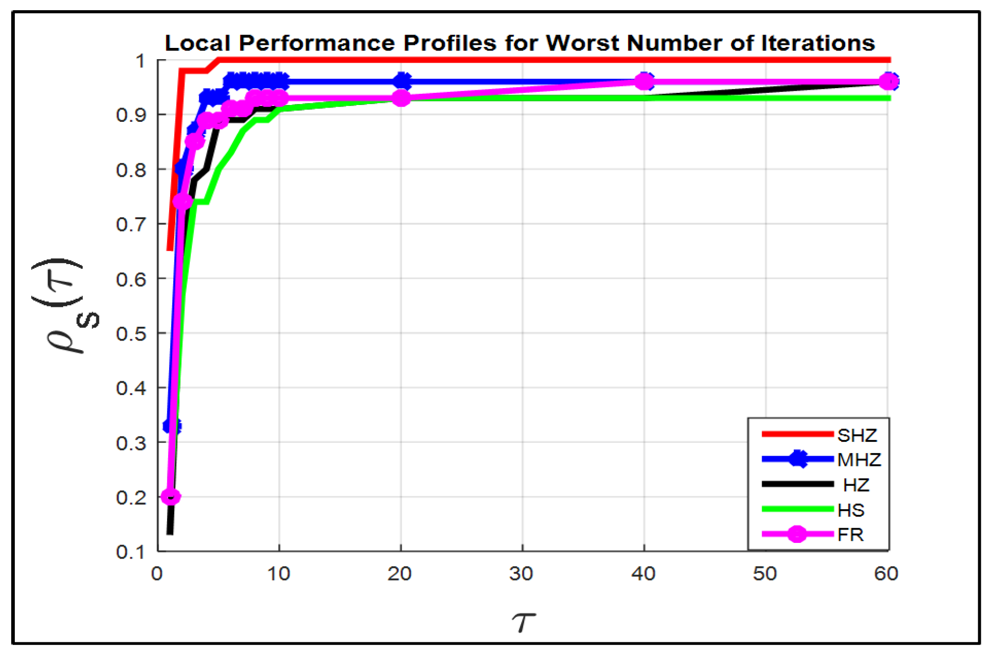
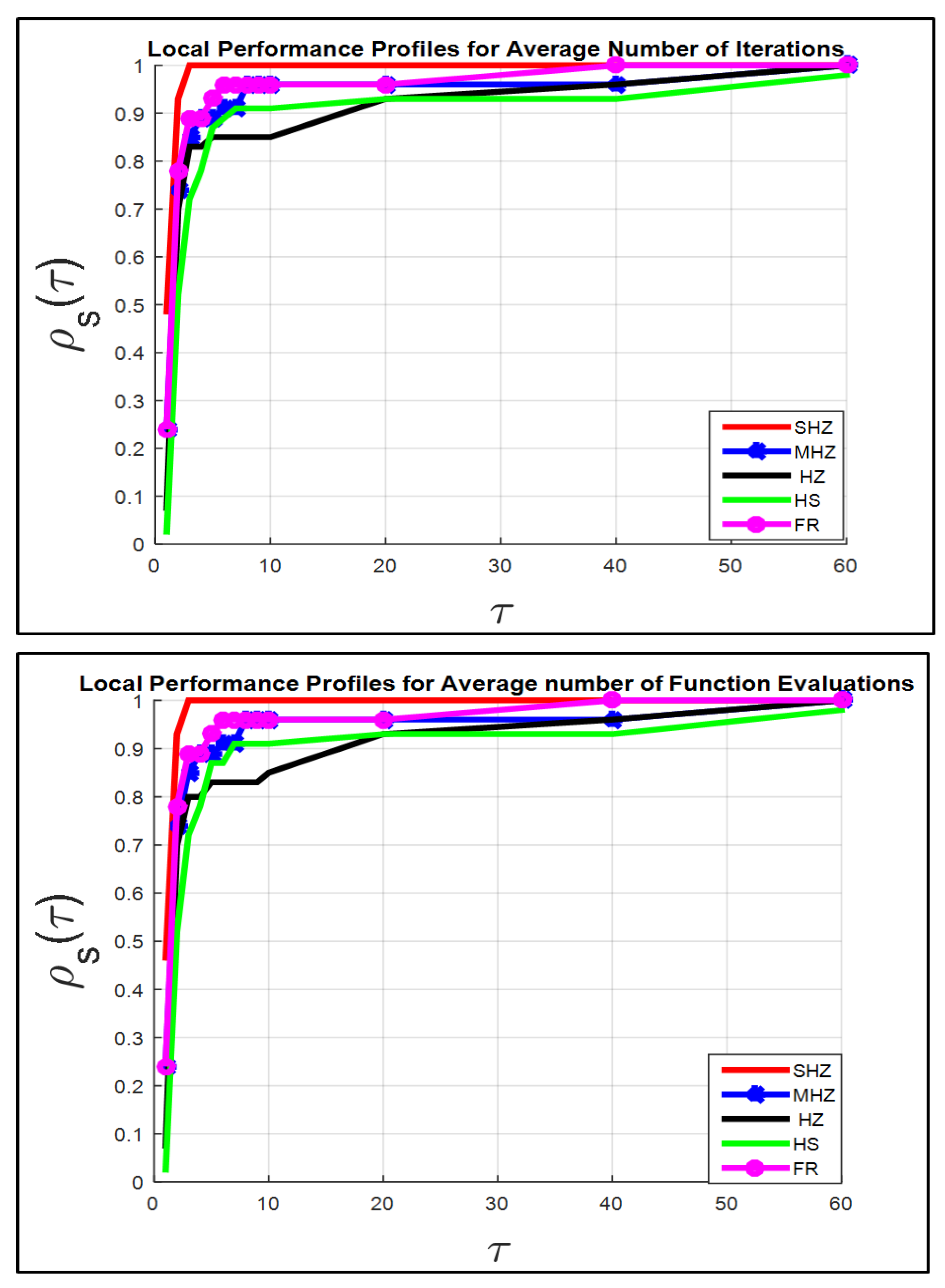
The performance profile depicted on the left of Figure 1 (in the term itr.w) compares the five techniques for a set of the 46 test problems.

The SHZ method has the best performance for the 46 test problems; this means that our suggested approach is capable of finding a local minimizer to the 46 test problems as fast as, or faster than, the other four approaches.

For instance, if  $\tau =1$, the  SHZ technique is capable of finding the local minimizer for $65\%$ of problems versus the $33\%$, $20\%$, $20\%$ and $13\%$ of a set of test problems solved by the MHZ, HS, FR and HZ methods, respectively.

In general, the  term itr.w, $\tau =60$ displays that all test problems are solved by SHZ against $96\%$ of test problems solved by the MHZ, HZ and FR methods respectively, while $93\%$ of test problems are solved by the HS method. At $\tau \ge 400$, all test problems are solved by the MHZ, HZ and FR methods respectively, while $98\%$ of test problems are solved by the HS.

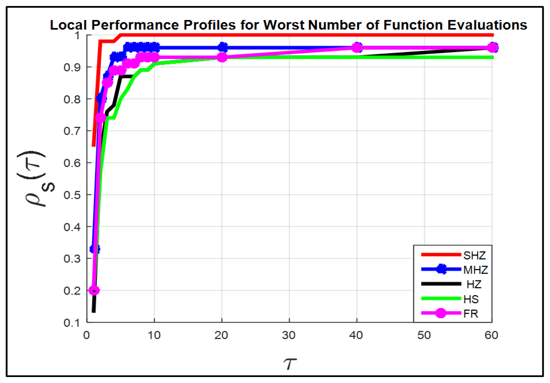
The right graph of Figure 1 shows that the method SHZ is capable of finding the local minimum of all test problems regarding term FEs.w.

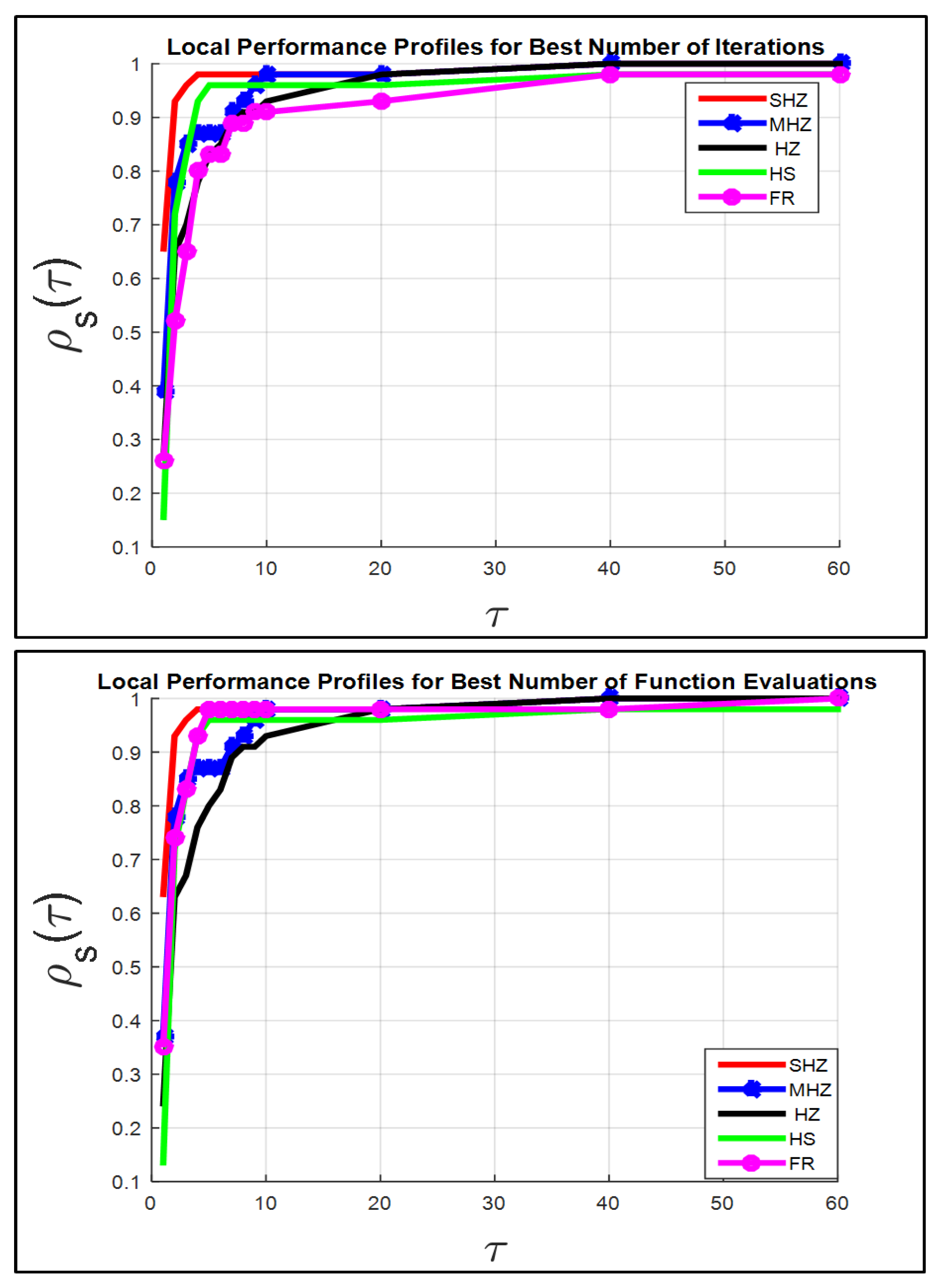
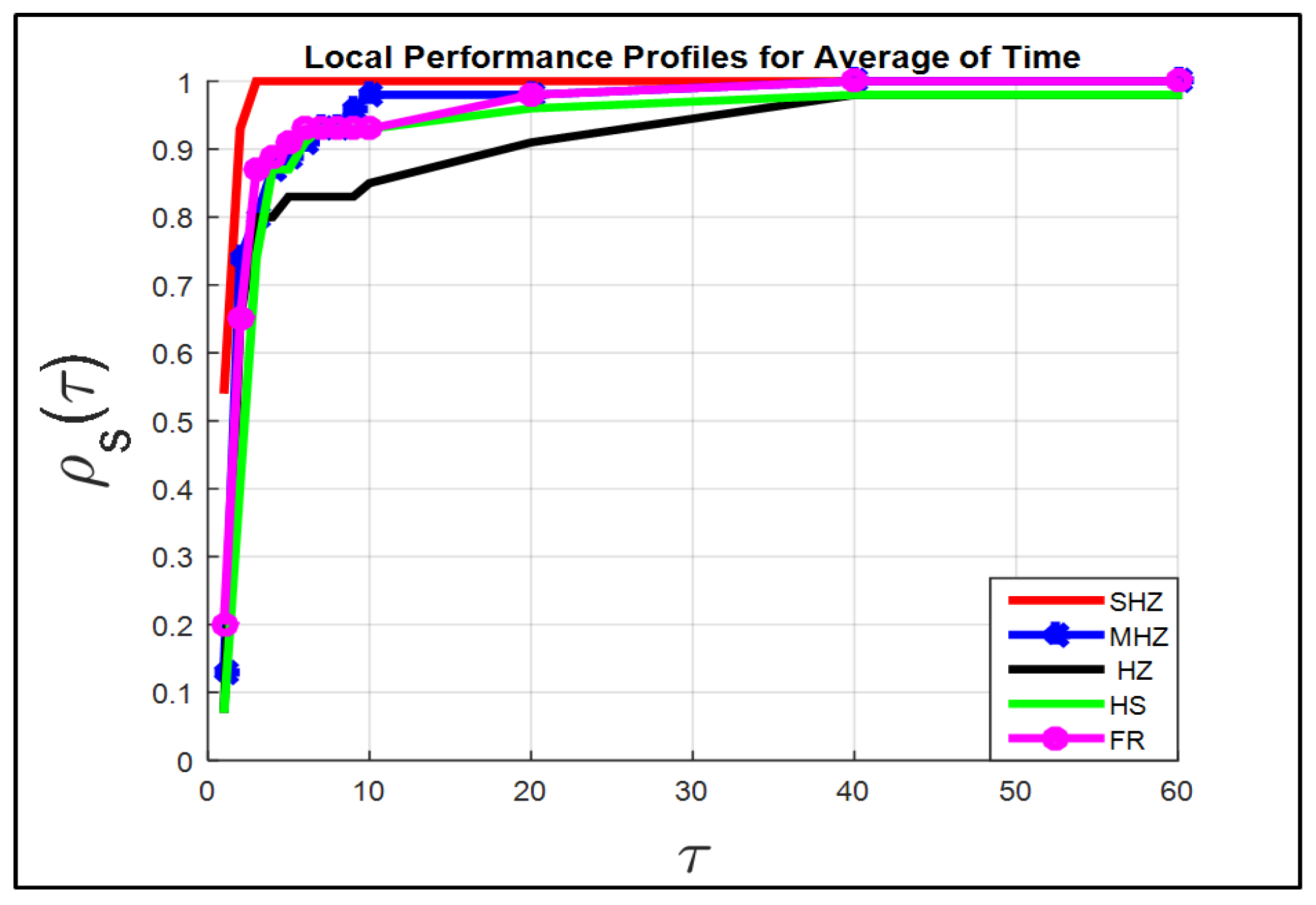
The rest of Figure 2, Figure 3 and Figure 4 show that the SHZ algorithm is superior to the four algorithms regarding the rest of the terms of the set Fit.

Therefore, the SHZ technique includes the characteristics of efficiency, reliability and effectiveness in solving Problem (1) compared to the other four methods.

Note: The power of the SHZ technique comes from the fact that the SHZ method gains the features of the four methods MHZ, HZ and HS, as we mentioned in Section 2.

Part II: Global Minimization Problem

It is worth mentioning that the final results of Part I for the second set of test problems contain some global minimizers at some runs for some non-convex functions. This means that the pure CG technique could not find the global minimizer of the second type of test problems for each run because it is a local method.

Therefore, to make this method capable of solving Problem (2) per run, the random technique is proposed and it is added to the CG approach to gain a new PS-CG hybrid technique that solves Problem (2). In many studies, the numerical outcomes indicated that the interbreed between a classical method and a random technique is very successful in overcoming the weakness of these methods. See [55,56,57,58,59].

Consequently, this part of the paper seeks to solve Problem (2).

Therefore, each method of the five CG methods mentioned in Part I is hybridized with the stochastic technique to obtain five algorithms to try to solve Problem (2).

In the next section, a stochastic technique is presented.

5. Random Technique

In this section, a new random parameter “SP” is presented. This stochastic technique contains three different formulas by which three different points are generated. This set of formulas is combined with the CG method to obtain a new algorithm that solves Problem (2).

Random Parameters (SP Technique)

Step 1: The first point is computed as follows, generate $V_{{}_k}\sim {[-1,1]}^n$ is as a random vector, set ${\gamma }_{{}_k}={10}^{{\psi }_{{}_k}}$, ${\psi }_{{}_k}\in [0.01,1)$, where the interval $[0.01,1)$ is divided into Itr of fractions and at every iteration k, the parameter ${\psi }_{{}_k}$ takes one value of the Itr and then computes ${\lambda }_{{}_{\mathit{k}}}=\frac{{(1+{\gamma }_{{}_k})}^{|{\mathit{V}}_{{}_{\mathit{i}}}|}}{{\gamma }_{{}_k}}S{\mathit{V}}_{{}_{\mathit{i}}}$ as a research direction with the step lengths, where $i=1,2,\dots ,n$, n is the of number variables, Itr is the number of iterations, and $S{\mathit{V}}_{{}_{\mathit{i}}}$ denotes the signs of the $\mathit{V}$ and is defined by

$$S{\mathit{V}}_{{}_{\mathit{i}}}=\left\{\begin{array}{cc}-1\hfill & \mathrm{if}{\mathit{V}}_{{}_{\mathit{i}}}<0,\hfill \\ 1\hfill & \mathrm{otherwise}.\hfill \end{array}\right.$$

(60)

Thus, a  point is calculated as follows:

$${\mathit{x}}_{{}_{\mathbf{1}}}={\mathit{x}}_{\mathit{ac}}+{\lambda }_{{}_{\mathit{k}}},$$

(61)

where ${\mathit{x}}_{\mathit{ac}}$ is the best point obtained yet, and then we compute $f_{{}_1}=f\left(x_{{}_1}\right)$.

Step 2: The second point is defined by

$${\mathit{x}}_{{}_{\mathbf{2}}}={\mathit{x}}_{{}_{\mathit{ac}}}+{\eta }_{{}_k}{\mathit{B}}_{{}_{\mathit{k}}},$$

(62)

where $B_{{}_k}={\phi }_{{}_k}{\mathit{d}}_{{}_{\mathit{k}}}$, ${\phi }_{{}_k}$ is defined by (47), ${\eta }_{{}_k}\in (0,2)$ is a random number, and the ${\mathit{d}}_{{}_{\mathit{k}}}$ is defined by (23). Then, we compute $f_{{}_2}=f\left({\mathit{x}}_{{}_{\mathbf{2}}}\right)$.

Step 3: This point is defined by

$${\mathit{x}}_{{}_{\mathbf{3}}}={\mathit{X}}_{{}_{\mathit{w}}}+\frac{1}{2}\mathit{Dx},$$

(63)

where $\mathit{Dx}=\frac{{(1+{\mu }_{{}_k})}^{|{\mathit{V}}_{{}_{\mathit{i}}}|}-1}{{\mu }_{{}_k}+0.1}S{\mathit{V}}_{{}_{\mathit{i}}}$, ${\mu }_{{}_k}={\left|f_{ac}\right|}^2$, $f_{ac}$ is the function value at the point $x_{ac}$ that has been accepted, and ${\mathit{X}}_{{}_{\mathit{w}}}$ is a stochastic variable picked from the feasible range of the objective function. This means that for ${\mathit{X}}_{{}_{\mathit{w}}}\sim {[a,b]}^n$, a and b are the lower and upper bounds of the feasible range, respectively, and the random vector $\mathit{V}$ with its signs $S{\mathit{V}}_{{}_{\mathit{i}}}$ is defined by the first step.

Therefore, we calculate $f_{{}_3}=f\left({\mathit{x}}_{{}_{\mathbf{3}}}\right)$.

For finding the global minimizer of a non-convex function, the above stochastic technique is used since Algorithm 1 is not capable of finding the global solution at each run. In other words, in some runs, Algorithm 1 fails to find the global solution to this function due to it sticking to a local point.

In the following example, we show how the SP algorithm is run.

Example: This example shows how the three steps of the SP algorithm are implemented.

We use the first test problem of the list of the test problems that are listed in Appendix A. $R_{{}_2}\left(x\right)=100{(x_{{}_1}^2-x_{{}_2})}^2+{(x_{{}_1}-1)}^2$, to facilitate an explanation of the mechanism of using the Sp algorithm (Formulas (61)–(63)), we use the following easy information about the function $R_{{}_2}\left(x\right)$, $n=2$ is the number of the variables, $x_{ac}=[2;-1]$, or $x_{ac}=[2;1]$, where $x_{ac}$ represents the best solution has been accepted so far or the starting point; hence, the function values at the two points are $R_{{}_2}\left(x_{ac}\right)=100{(2^2+1)}^2+{(2-1)}^2=2500+1=2501$ and $R_{{}_2}\left(x_{ac}\right)=100{(2^2-1)}^2+{(2-1)}^2=900+1=901$.

Supposing $Itr=5$ is the number of iterations, the interval $[0.01;1)$ is divided into five fractions with step size $\frac{1-0.01}{5}=0.198$, and thus the set of this fractions is $A=\{0.01,0.208,0.406,0.604,0.802\}$, let k be 3 which means the algorithm is at the third iteration. Then, ${\psi }_{{}_3}=0.406$, ${\gamma }_{{}_3}={10}^{{\psi }_{{}_3}}={10}^{0.406}=2.5468$. Let $V_{{}_3}$ be $[-0.5;1]$, then ${\lambda }_{{}_{\mathbf{3}}}=\left[\frac{{(1+2.5468)}^{|-\mathbf{0}.\mathbf{5}|}}{2.5468}\times -1;\frac{{(1+2.5468)}^{\left|\mathbf{1}\right|}}{2.5468}\times 1\right]=\left[-\frac{1.8833}{2.5468};\frac{3.5468}{2.5468}\right]=\left[-0.73948;1.3926\right].$

Therefore, the new solution is computed by Formula (61) as follows.

$x_{{}_1}=x_{ac}+{\lambda }_{{}_3}=[2;-1]+[-0.73948;1.3926]=[1.2605;0.3926]$ or $x_{{}_1}=x_{ac}+{\lambda }_{{}_3}=[2;1]+[-0.73948;1.3926]=[1.2605;2.3926]$.

The function values at both points are as follows.

$R_{{}_2}\left(x_{{}_1}\right)=100{(1.{2605}^2-0.3926)}^2+{(1.2605-1)}^2=143.1+0.06786=143.17$ or $R_{{}_2}\left(x_{{}_1}\right)=100{(1.{2605}^2-2.3926)}^2+{(1.2605-1)}^2=64.6+0.06786=64.668$.

Therefore, $R_{{}_2}\left(x_{{}_1}\right)<R_{{}_2}\left(x_{ac}\right)$; this means the solution that is generated by Formula (61) reduces the function value.

In the following, we explain how the candidate solution is generated by Formula (62).

Let $M_{{}_{ϵ}}=1.2\times {10}^{-6}$. By using Formula (45), we obtain $h_{{}_3}=4.381\times {10}^{-5}$ as the step size h (a random interval) to the difference approximations method, and then we have $x_{{{}_h}_{{}_1}}=[x_{ac}\left(1\right)+h_{{}_3};x_{ac}\left(2\right)]=[2+4.381\times {10}^{-5};-1]$, $x_{{{}_h}_{{}_2}}=[x_{ac}\left(1\right);x_{ac}\left(2\right)+h_{{}_3}]=[2;-1+4.381\times {10}^{-5}]$.

Therefore, the values of the function at the three points $x_{ac}$, $x_{{{}_h}_{{}_1}}$ and $x_{{{}_h}_{{}_2}}$ are listed in the following.

$R_{{}_2}\left(x_{ac}\right)=2501$, $R_{{}_2}\left(x_{{{}_h}_{{}_1}}\right)=2501.175$ and $R_{{}_2}\left(x_{{{}_h}_{{}_2}}\right)=2500.956$.

We compute the approximate value of the gradient vector by Formula (46) as follows:

$$DFF\left(x_{ac}\right)=\left[\frac{2501.175-2501}{4.381\times {10}^{-5}};\frac{2500.956-2501}{4.381\times {10}^{-5}}\right]=\left[3994.522;-1004.34\right],$$

${\phi }_{{}_3}=\frac{2501}{{\parallel \mathit{DFF}\parallel }^2}=0.0002$, where ${\phi }_{{}_3}$ is defined by (47).

We consider $d_{{}_3}=-g\left(x_{ac}\right)\approx \left[-3994.522;1004.34\right]$ because we do not have information about the value of the $d_{{}_2}$ in this illustration example.

Now, we apply Formula (62), as follows $B_{{}_3}={\phi }_{{}_3}{d}_{{}_2}=[-0.799;0.201]$, we take ${\eta }_{{}_3}=0.971$ as a random number from the range $(0,2)$, then $x_{{}_2}=[2;-1]+0.971\times [-0.799;0.201]=[1.2242;-0.80483]$, the function value at the point $x_{{}_2}$ is $R_{{}_2}\left(x_{{}_2}\right)=530.66$.

We note that the $R_{{}_2}\left(x_{{}_2}\right)=530.66<R_{{}_2}\left(x_{ac}\right)=2501$, i.e., the function value is reduced by the point $x_{{}_2}$.

In the following, we explain how the candidate solution is generated by Formula (63).

${\mu }_{{}_3}={\left|f_{ac}\right|}^2={2501}^2=6,255,001$, $\mathit{Dx}=\left[\frac{{(1+6,255,001)}^{|-0.5|}-1}{6,255,001+0.1}\times -1;\frac{{(1+6,255,001)}^{\left|1\right|}-1}{6,255,001+0.1}\times 1\right]=\left[-\frac{2501-1}{6,255,001.1};\frac{6,255,002-1}{6,255,001.1}\right]=\left[-0.0004;0.999\right].$${\mathit{X}}_{{}_{\mathit{w}}}=[-3.095;8.701]$ is as a random vector picked from the range ${[-5,10]}^2$, and then $x_{{}_3}=[-3.095;8.701]+\frac{1}{2}[-0.0004;0.999]=[-3.095;8.701]+[-0.0002;0.4995]=[-3.0952;9.2005]$.

We compute the function value at the point $x_{{}_3}$; $R_{{}_2}\left(x_{{}_3}\right)=100{({(-3.0952)}^2-9.2005)}^2+{(-3.0952-1)}^2=14.422+16.771=31.193$.

We note that the $R_{{}_2}\left(x_{{}_3}\right)=31.193<R_{{}_2}\left(x_{ac}\right)=2501$. Therefore, the point $x_{{}_3}$ minimizes the function value.

According to the above example that illustrates the mechanism of Formulas (61)–(63), we deduce the following results.

Remark 1.

Formulas (3), (61) and (62) are the main formulas which are used in the new hybrid proposed algorithm that is described in Section 6. However, Formula (63) is used when $\Delta f=0$ that is defined by Formula (25); in this case, Algorithm 3 reaches a critical point, thus if this point is the approximate value of the global minimizer point of the f, then Algorithm 3 stops according to the condition in Line 4 or Line 1 of Algorithm 3. Otherwise, the candidate solution is generated by Formula (63); see Section 6. Consequently, in this example, at iteration $k=3$, the result which is obtained by Formula (63) cannot be taken into account due to the $\Delta f\ne 0$.

Remark 2.

All Formulas (61)–(63) minimize the function value from any starting point.

6. Hybridization of the CG Method with Stochastic Parameters

When a stochastic method as a global optimization algorithm is combined with a globally convergent method (deterministic method), the result is a global optimization algorithm [55,56].

Therefore, the SP technique is hybridized with each of the five conjugate gradient methods SHZ, MHZ, HZ, HS and FR to obtain five techniques.

Our proposed algorithm is called a hybrid stochastic CG method abbreviated by HSSHZ that solves Problem (2). However, Algorithm 3 represents five alternative algorithms when the SHZ method is hybridized with the PS technique, then we obtain a new algorithm abbreviated by HSSHZ. When we combine any method of MHZ, HZ, HS or FR, we obtain four other abbreviations of algorithms as follows: HSMHZ, HSHZ, HSHS and HSFR, respectively.

In general, the outputs of this paper are five algorithms that solve Problem (2), where the best one is the HSSHZ algorithm as illustrated by the numerical experiments section of Part II.

In the following, Algorithm 1 is combined with SP technique to obtain Algorithm 3.

The SP method permits conducting an exhaustive wipe of the search range to guarantee that the global minimizer point is visited at least once per run.

Algorithm 3 Hybrid stochastic CG method.

Input:  $f:{\mathbb{R}}^n\to \mathbb{R}$, $f\in C^1$, $f_{ac}=f_{{}_{cg}}$ gained by Algorithm 1 and $\epsilon >0$. Output:  ${\mathit{x}}_{{}_{\mathit{gl}}}={\mathit{x}}_{{}_{\mathit{ac}}}$ the global minimizer of f, $f\left({\mathit{x}}_{{}_{\mathit{gl}}}\right)$, the value of f at ${\mathit{x}}_{{}_{\mathit{gl}}}$. 1: while$|f_{{}_{ac}}-f^{*}|>\epsilon$ or FEs$<n{10}^4$ do 2:     $f_{cg}$ is a function value f gained by Algorithm 1. 3:     $f_{ac}=min\{f_{cg},f_{{}_1},f_{{}_2}\}$ and $x_{ac}$ the best point gives the $f_{ac}$. 4:     if $|f_{{}_{ac}}-f^{*}|\le \epsilon$ then 5:         Stop. 6:     end if 7:     if $▵f==0$ then 8:         calculate the ${\mathit{x}}_{{}_{\mathbf{3}}}$ and the $f_{{}_3}=f\left({\mathit{x}}_{{}_{\mathbf{3}}}\right)$ by Formula (63). 9:         if $f_{{}_3}<f_{ac}$ then 10:            the ${\mathit{x}}_{{}_{\mathbf{3}}}$ is accepted, compute the ${\mathit{x}}_{\mathit{ac}}\to {\mathit{x}}_{{}_{\mathbf{3}}}$, $f_{ac}\to f_{{}_3}$, and go to Line 1. 11:         else 12:            generate another point ${\mathit{x}}_{{}_{\mathbf{3}}}$ by Formula (63). 13:         end if 14:     else 15:         go to Line 1. 16:     end if 17: end while 18: return${\mathit{x}}_{\mathit{ac}}$ the best point and its function value $f_{ac}$

A Mechanism Running Algorithm 3

As we mentioned above, Algorithm 3 is a combination of two methods; the first is a CG method of the five techniques CG $=\{SHZ,MHZ,HZ,SH,FR\}$ that are discussed in Part I, and the second is a random method is depicted by Section 5. The point ${\mathit{x}}_{{}_{\mathit{cg}}}$ is obtained by Algorithm 1 and it will be an input to Algorithm 3.

Algorithm 3 begins with Line 1 that is the stopping standard of the algorithm. Therefore, Algorithm 3 ends if one of the following standards is satisfied: The first standard is $|f_{{}_{ac}}-f^{*}|\le \epsilon$, and the second standard is FEs $\ge n{10}^4$, where $f_{{}_{ac}}$ the best value of the function f is gained, the $f^{*}$ is the true solution, $\epsilon ={10}^{-6}$, FEs is the number of function evaluations, and FEs $=n{10}^4$ is a stopping standard indicated by [85,86].

In Line 3, the best value of f is selected from the three values of the function $f_{cg}$, $f_{{}_1}$ and $f_{{}_2}$, and indicated by $f_{ac}$, the three values of the function f are calculated by Algorithms (1), (61) and (62), respectively, and ${\mathit{x}}_{\mathit{ac}}$ indicates this.

In Line 4, if $|f_{{}_{ac}}-f^{*}|\le \epsilon$ is fulfilled, the algorithm ends. The standard that is listed in Line 7 gives the algorithm an opportunity to flee from the local points. Consequently, if $▵f=0$, then the algorithm has reached a crucial point. Therefore, if the norm of the gradient vector is 0 or ≈0, this point is either a local point or the global point. According to the above actions, the hybrid algorithm has been granted sequential opportunities to escape out of a snare (a local point). Thus, the procedures in Lines 8–12 are eligible for helping the algorithm to flee this snare, especially since the second stopping standard guarantees that most of the research domain is scanned.

The numerical outcomes of the five methods are given in the next section.

7. Numerical Experiments of Part II

The numerical results for the second test problems (non-convex functions) are presented, and these results are obtained by Algorithm 3.

The performance profiles tool that is described in Part I is used here for assessing the achievement of Algorithm 3 that contains five alternatives of algorithms as we mentioned above in Section 6.

The numerical results of the second type of the test problems are listed in

Table 9. The number of worst iterations.

f	n	HSSHZ	HSMHZ	HSHZ	HSHS	HSFR	f	n	HSSHZ	HSMHZ	HSHZ	HSHS	HSFR
$S{5}^{*}$	4	3150	55	85	F	F	$S{7}^{*}$	4	10,000	F	10,000	F	F
$S{10}^{*}$	4	710	F	3020	F	F	$H{M}^{*}$	2	40	100	95	75	180
$H^{*}$	3	300	590	1155	465	1270	$H^{*}$	6	50	500	300	9550	F
$C{B}^{*}$	2	55	145	15	200	90	$P{8}^{*}$	4	20	15	15	550	10
$P{16}^{*}$	5	755	835	3280	F	7300	$S{H}^{*}$	2	100	115	200	250	190
$Bh{1}^{*}$	2	205	F	F	F	F	$Ra{s}^{*}$	2	1310	F	F	F	F
$G{P}^{*}$	2	20	F	F	300	F	$L{e}^{*}$	10	2470	1430	F	F	3100

,

Table 10. The number of worst function evaluations.

f	n	HSSHZ	HSMHZ	HSHZ	HSHS	HSFR	f	n	HSSHZ	HSMHZ	HSHZ	HSHS	HSFR
$S{5}^{*}$	4	12,600	220	340	F	F	$S{7}^{*}$	4	40,000	F	40,000	F	F
$S{10}^{*}$	4	2840	F	12,080	F	F	$H{M}^{*}$	2	120	200	190	150	360
$H^{*}$	3	900	1770	3465	1395	3810	$H^{*}$	6	300	3000	1800	57,300	F
$C{B}^{*}$	2	110	290	30	400	180	$P{8}^{*}$	4	80	60	60	2200	40
$P{16}^{*}$	5	3775	4175	16,400	F	36,500	$S{H}^{*}$	2	200	230	400	500	380
$Bh{1}^{*}$	2	410	F	F	F	F	$Ra{s}^{*}$	2	2620	F	F	F	F
$G{P}^{*}$	2	40	F	F	600	F	$L{e}^{*}$	10	24,700	14,300	F	F	31,000

,

Table 11. The number of best iterations.

f	n	HSSHZ	HSMHZ	HSHZ	HSHS	HSFR	f	n	HSSHZ	HSMHZ	HSHZ	HSHS	HSFR
$S{5}^{*}$	4	50	35	55	F	F	$S{7}^{*}$	4	750	F	520	F	F
$S{10}^{*}$	4	20	F	70	F	F	$H{M}^{*}$	2	15	10	10	10	5
$H^{*}$	3	50	60	85	20	130	$H^{*}$	6	50	100	100	50	F
$C{B}^{*}$	2	15	10	10	50	10	$P{8}^{*}$	4	5	5	5	50	5
$P{16}^{*}$	5	150	35	80	F	40	$S{H}^{*}$	2	10	10	10	50	10
$Bh{1}^{*}$	2	20	F	F	F	F	$Ra{s}^{*}$	2	10	F	F	F	F
$G{P}^{*}$	2	15	F	F	50	F	$L{e}^{*}$	10	400	120	F	F	395

,

Table 12. The number of best function evaluations.

f	n	HSSHZ	HSMHZ	HSHZ	HSHS	HSFR	f	n	HSSHZ	HSMHZ	HSHZ	HSHS	HSFR
$S{5}^{*}$	4	200	140	220	F	F	$S{7}^{*}$	4	3000	F	2080	F	F
$S{10}^{*}$	4	80	F	280	F	F	$H{M}^{*}$	2	45	20	20	20	10
$H^{*}$	3	150	180	255	60	390	$H^{*}$	6	300	600	600	300	F
$C{B}^{*}$	2	30	20	20	100	20	$P{8}^{*}$	4	20	20	20	200	20
$P{16}^{*}$	5	725	175	400	F	200	$S{H}^{*}$	2	20	20	20	100	20
$Bh{1}^{*}$	2	40	F	F	F	F	$Ra{s}^{*}$	2	20	F	F	F	F
$G{P}^{*}$	2	30	F	F	100	F	$L{e}^{*}$	10	4000	1200	F	F	3950

,

Table 13. The average of time.

f	n	HSSHZ	HSMHZ	HSHZ	HSHS	HSFR	f	n	HSSHZ	HSMHZ	HSHZ	HSHS	HSFR
$S{5}^{*}$	4	0.720	0.050	0.046	F	F	$S{7}^{*}$	4	7.368	F	13.249	F	F
$S{10}^{*}$	4	0.151	F	0.885	F	F	$H{M}^{*}$	2	0.017	0.031	0.028	0.021	0.053
$H^{*}$	3	0.186	0.353	0.409	0.271	0.361	$H^{*}$	6	0.057	0.194	0.143	4.712	F
$C{B}^{*}$	2	0.018	0.025	0.010	0.049	0.030	$P{8}^{*}$	4	0.014	0.015	0.009	0.116	0.007
$P{16}^{*}$	5	0.319	0.135	0.683	F	1.606	$S{H}^{*}$	2	0.028	0.037	0.050	0.084	0.039
$Bh{1}^{*}$	2	0.039	F	F	F	F	$Ra{s}^{*}$	2	0.261	F	F	F	F
$G{P}^{*}$	2	0.015	F	F	0.078	F	$L{e}^{*}$	10	1.221	0.627	F	F	2.087

,

Table 14. The average of number of iterations.

f	n	HSSHZ	HSMHZ	HSHZ	HSHS	HSFR	f	n	HSSHZ	HSMHZ	HSHZ	HSHS	HSFR
$S{5}^{*}$	4	416.7	47	67	F	F	$S{7}^{*}$	4	5928.7	F	8648	F	F
$S{10}^{*}$	4	131.3	F	589	F	F	$H{M}^{*}$	2	24.3	29	34.8	25.8	50.8
$H^{*}$	3	213.3	268.8	373.3	247	333.8	$H^{*}$	6	50	205	177.5	2382.5	F
$C{B}^{*}$	2	26	23.3	12.8	57.5	36.8	$P{8}^{*}$	4	12	11	10.5	267.5	6.3
$P{16}^{*}$	5	376	171.25	878.8	F	2208.5	$S{H}^{*}$	2	30.3	39	48.5	65	41.5
$Bh{1}^{*}$	2	74.3	F	F	F	F	$Ra{s}^{*}$	2	346.7	F	F	F	F
$G{P}^{*}$	2	18	F	F	62.5	F	$L{e}^{*}$	10	1012.7	506	F	F	1380.3

and

Table 15. The average of number of function evaluations.

f	n	HSSHZ	HSMHZ	HSHZ	HSHS	HSFR	f	n	HSSHZ	HSMHZ	HSHZ	HSHS	HSFR
$S{5}^{*}$	4	1666.7	188	268	F	F	$S{7}^{*}$	4	23,714.7	F	34,592	F	F
$S{10}^{*}$	4	525.3	F	2356	F	F	$H{M}^{*}$	2	73	58	69.5	51.5	101.5
$H^{*}$	3	640	806.3	1119.8	741	1001.3	$H^{*}$	6	300	1230	1065	14,295	F
$C{B}^{*}$	2	52	46.5	25.5	115	73.5	$P{8}^{*}$	4	48	44	42	1070	25
$P{16}^{*}$	5	1880	856.3	4393.8	F	11,042.5	$S{H}^{*}$	2	60.7	78	97	130	83
$Bh{1}^{*}$	2	148.7	F	F	F	F	$Ra{s}^{*}$	2	693.3	F	F	F	F
$G{P}^{*}$	2	36	F	F	125	F	$L{e}^{*}$	10	10,126.7	5060	F	F	13,802.5

. Columns 1–2 and 8–9 contain the abbreviation of the function f and the number of the unknowns n, respectively. Columns 3–7 contain the abbreviation of each algorithm of the five algorithm HSSHZ, HSMHZ, HSHZ, HSHS and HSFR, which present the number of worst iterations, number of worst function evaluations, number of best iterations, number of best function evaluations, average of time (CPU), average of number of iterations and average of number of function evaluations, respectively. Columns 10–14 are similar to Columns 3–7.

Note: F denotes that the algorithm has failed to find the local minimizer of the function f according to the stopping criteria of Algorithm 3 which are listed in Section 6.

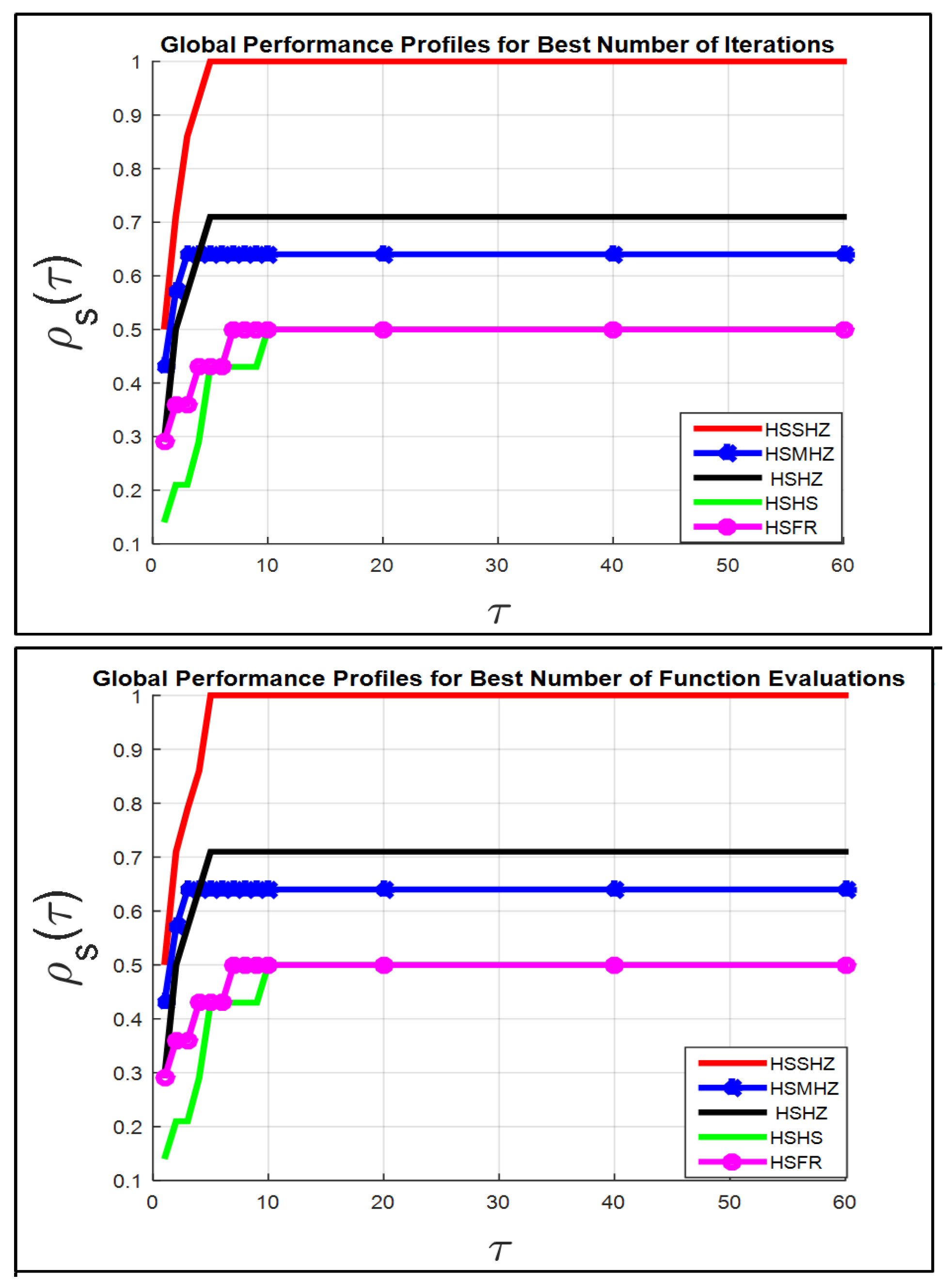
The performance profiles for the five algorithms are analyzed as follows.

Figure 5, Figure 6, Figure 7 and Figure 8 show the performance profiles of the five set solvers S regarding the set standard Fit that is mentioned in Section 4.2.

The performance profiles which are drawn on the left of Figure 5 (in the term itr.w) compares 5 methods for the 14 test problems.

The HSSHZ technique has a good achievement (for the term itr.w) for all test problems, which indicates that the HSSHZ technique is capable of solving Problem (2) as fast as or faster than the four techniques.

For instance, if $\tau =1$, the HSSHZ algorithm solves $71\%$ of the 14 test problems against $14\%$, $14\%$, $7\%$ and $0\%$, of the 14 test problems solved by the HSMHZ, HSHZ, HSFR and HSHS algorithms, respectively.

In general, for the term itr.w, $\tau \ge 60$ exhibits that the second type of the test problems are solved by HSSHZ, while $64\%$, $71\%$, $43\%$ and $50\%$ of test problems are solved by the HSMHZ, HSHZ, HSHS and HSFR algorithms respectively.

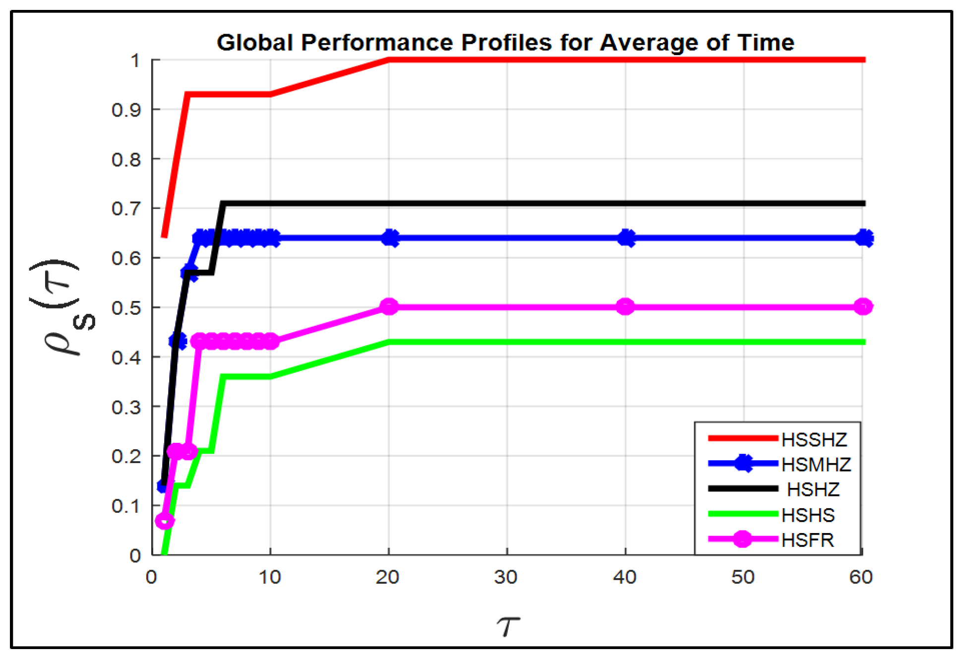
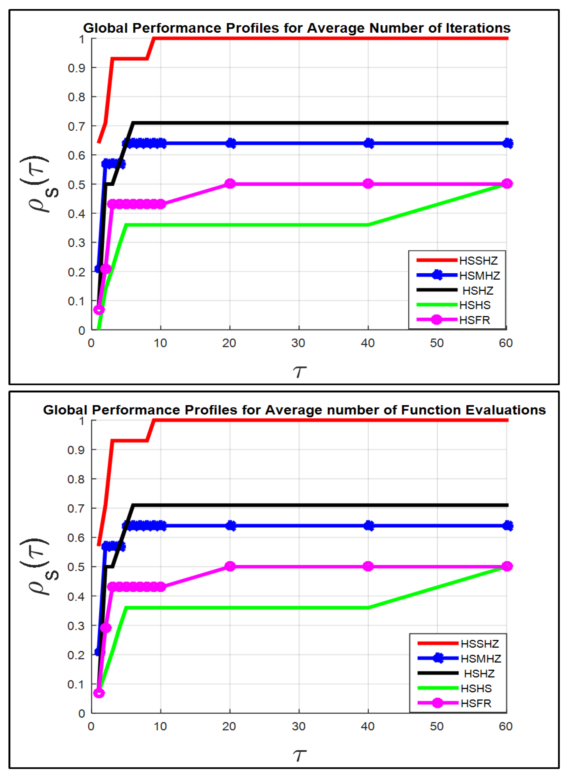
Figure 5, Figure 6, Figure 7 and Figure 8 demonstrate that the performance of the HSSHZ technique is better than the performance of the four techniques regarding the seven standards listed in the set Fit, respectively.

Therefore, the HSSHZ technique includes the characteristics of efficiency, reliability and effectiveness in finding the global minimizer of the non-convex function f compared to the other four methods.

It is worth observing that the power of the HSSHZ algorithm comes from the fact that the SHZ method gains the features of the four methods, MHZ, HZ, HS and FR, as mentioned in Section 2.

Note 1: In Algorithm 3, a run is considered successful if Inequality (64) is met.

$$|f_{{}_{ac}}-f^{*}|\le {10}^{-5},$$

(64)

where $f^{*}$ is the exact global solution that is listed in Columns 3 and 7 of Table 1, respectively, and the $f_{{}_{ac}}$ is the final result obtained by Algorithm 3.

Note 2: Formula (56) means if the final result $f_{{}_{ac}}$, obtained by Algorithm 3 satisfies Inequality (64), then the first branch of (56) is computed; otherwise, we set $r_{p,s}=\infty$.

8. Conclusions and Future Work

A new modified CG algorithm is suggested, named SHZ. The SHZ finds the local minimizers of unconstrained optimization problems. The modernized formulae of the SHZ algorithm are more complicated than previous approaches; nevertheless, the numerical experiments of the SHZ are very strong. The convergence analysis of the SHZ algorithm is designed. We also analyzed the gradient approximation $\mathit{g}\left(\mathit{x}\right)\approx$ DFF constructed by finite differences (the forward differences method). This method includes a new approach for selecting the fit value of the h according to the value of the objective function and it is updated dynamically at each iteration. The numerical results demonstrate that the performance of the SHZ method is positively competitive with the other four conjugate gradient methods based on performance profiles.

Comparing the final results of the gradient vector that were obtained by the method DFF to the exact values of the gradient vector demonstrates that the fresh technique succeeded in picking the right value of h. The proposed random approach recreates a critical role to make the SHZ method capable of finding the global minimizers of unconstrained optimization test problems, especially when the objective function is non-convex.

It can be worth observing that the power of the HSSHZ algorithm comes from the fact that the SHZ method gains the characteristics of the four methods, MHZ, HZ, HS and FR.

The suggested approach can be improved and modified to deal with constrained, multi-objective optimization problems, and it will be used for image restorations.