


Feature Selection and Classification of Transformer Faults Based on Novel Meta-Heuristic Algorithm
 , ,
, ,  ,
,  , and
, and 
Abstract
:1. Introduction
- A novel Gravitational Search Dipper Throated Optimization Algorithm (GSDTO) is proposed.
- A binary GSDTO algorithm, a binary version of the proposed algorithm, is applied for feature selection from the tested dataset.
- A GSDTO+LSTM classifier, based on the proposed GSDTO algorithm and LSTM method, is developed to improve the tested dataset classification accuracy.
- The GSDTO algorithm’s statistical difference is tested by Wilcoxon’s rank-sum and ANOVA tests.
- The GSDTO algorithm is used to improve the LSTM classification method performance for classifying purposes which can be applied in a new high voltage engineering application.
- The binary GSDTO algorithm and the LSTM-based classification algorithm can be generalized and tested for various types of datasets.
2. Materials and Methods
2.1. Distribution of the Data
2.2. Machine Learning
2.3. Dipper Throated Optimization (DTO)
2.4. Gravitational Search Algorithm (GSA)
| Algorithm 1 DTO Algorithm. |
|
| Algorithm 2 GSA Algorithm. |
|
1: Initialization positions of agents with n agents, maximum iterations , objective function , parameters of , , 2: Obtain for each agent 3: Find best agent 4: while do 5: for () do 6: Update gravitational and inertia masses by Equations (19) and (20) 7: Update acceleration of current agent by 8: Update acceleration of current agent by 9: Update position of current agent by 10: end for 11: Obtain for each agent 12: Update , , 13: Find best agent 14: Set = 15: end while 16: Return |
3. Proposed Methodology
3.1. Proposed GSDTO Algorithm
| Algorithm 3 Proposed GSDTO Algorithm. |
|
1: Initialization positions of agents with n agents, velocities of agents , maximum number of iterations , objective function , parameters of , , , , , , , C, R, , , , 2: Obtain for each agent 3: Find best agent 4: Set = 5: while do 6: if () then 7: for () do 8: if () then 9: Update current swimming agent position by 10: else 11: Update current flying agent velocity by 12: Update current flying agent position by 13: end if 14: end for 15: else 16: for () do 17: Update gravitational and inertia masses by Equations (29) and (30) 18: Update acceleration of current agent by 19: Update velocity of current agent by Equation (27) 20: Update position of current agent by Equation (26) 21: end for 22: end if 23: Obtain for each agent 24: Update , , C, R, , , 25: Find best agent 26: Set = 27: Set 28: end while 29: Return best agent |
- Initialize parameters of the GSDTO algorithm, , , , , , , , , , , C, R, , , , and : O(1).
- Calculate for each agent : O(n).
- Obtain the best agent : O (n).
- Update current swimming agent position: O().
- Update current flying agent velocity: O().
- Update current flying agent position: O().
- Update acceleration of current agent : O().
- Update velocity of current agent : O().
- Update position of current agent : O().
- Calculate for each agent : O().
- Update , , C, R, , , : O().
- Obtain best agent : O().
- Set = : O().
- Set : O().
- Obtain global best agent : O(1)
3.2. Proposed Binary GSDTO Algorithm
| Algorithm 4 Proposed Binary GSDTO Algorithm. |
|
3.3. Proposed GSDTO+LSTM Based Model
4. Experimental Results
4.1. Feature Selection Scenario
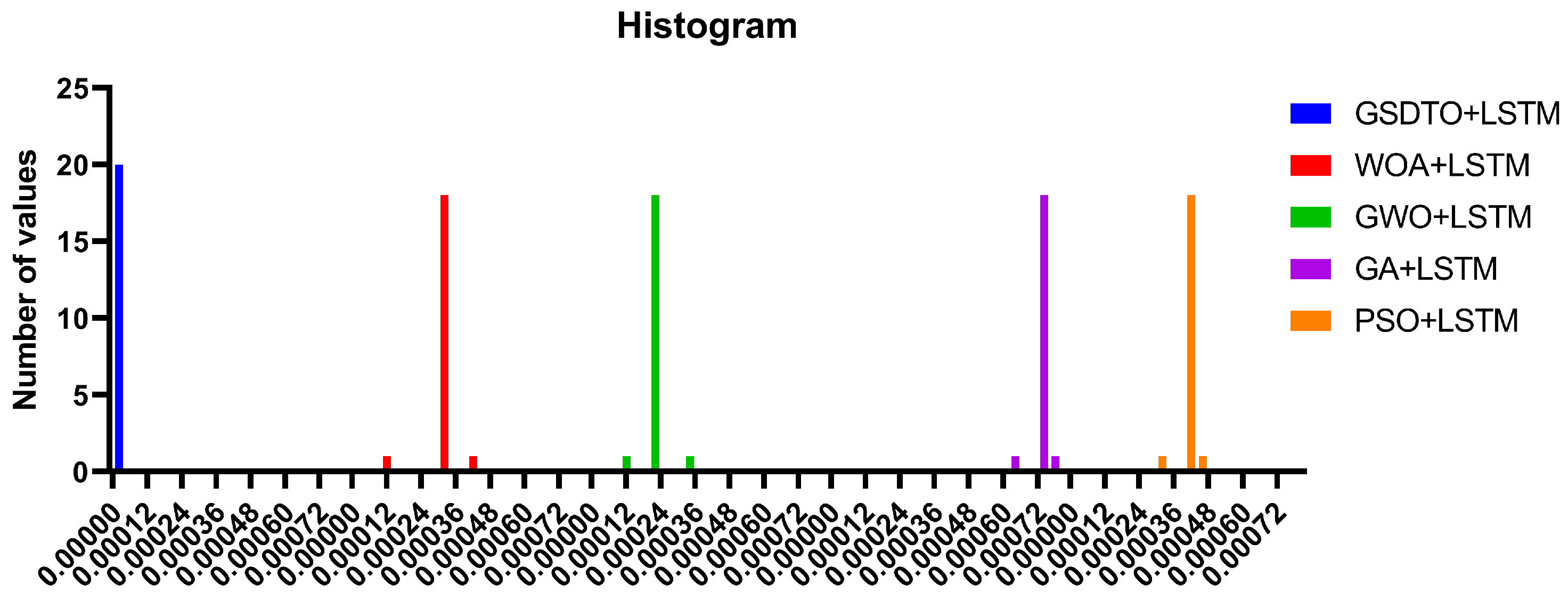
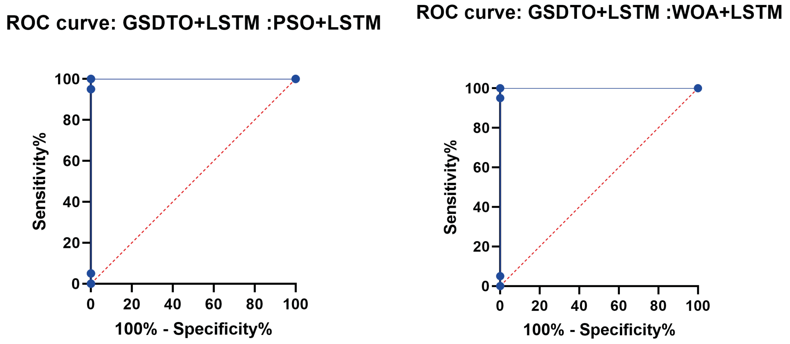
4.2. Classification Scenario
4.3. Validation and Discussion
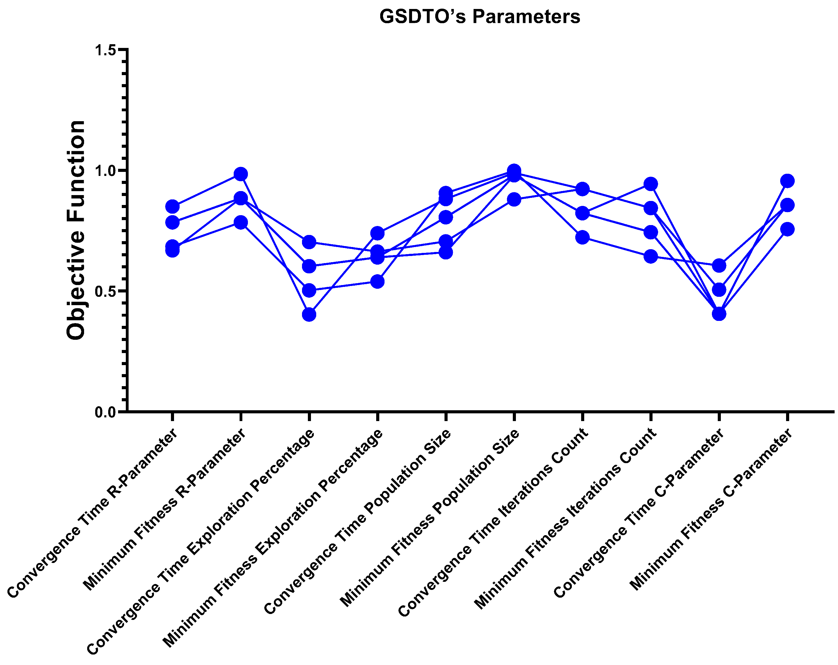
5. Sensitivity Analysis of the GSDTO Parameters
5.1. One-at-a-Time Sensitivity Analysis
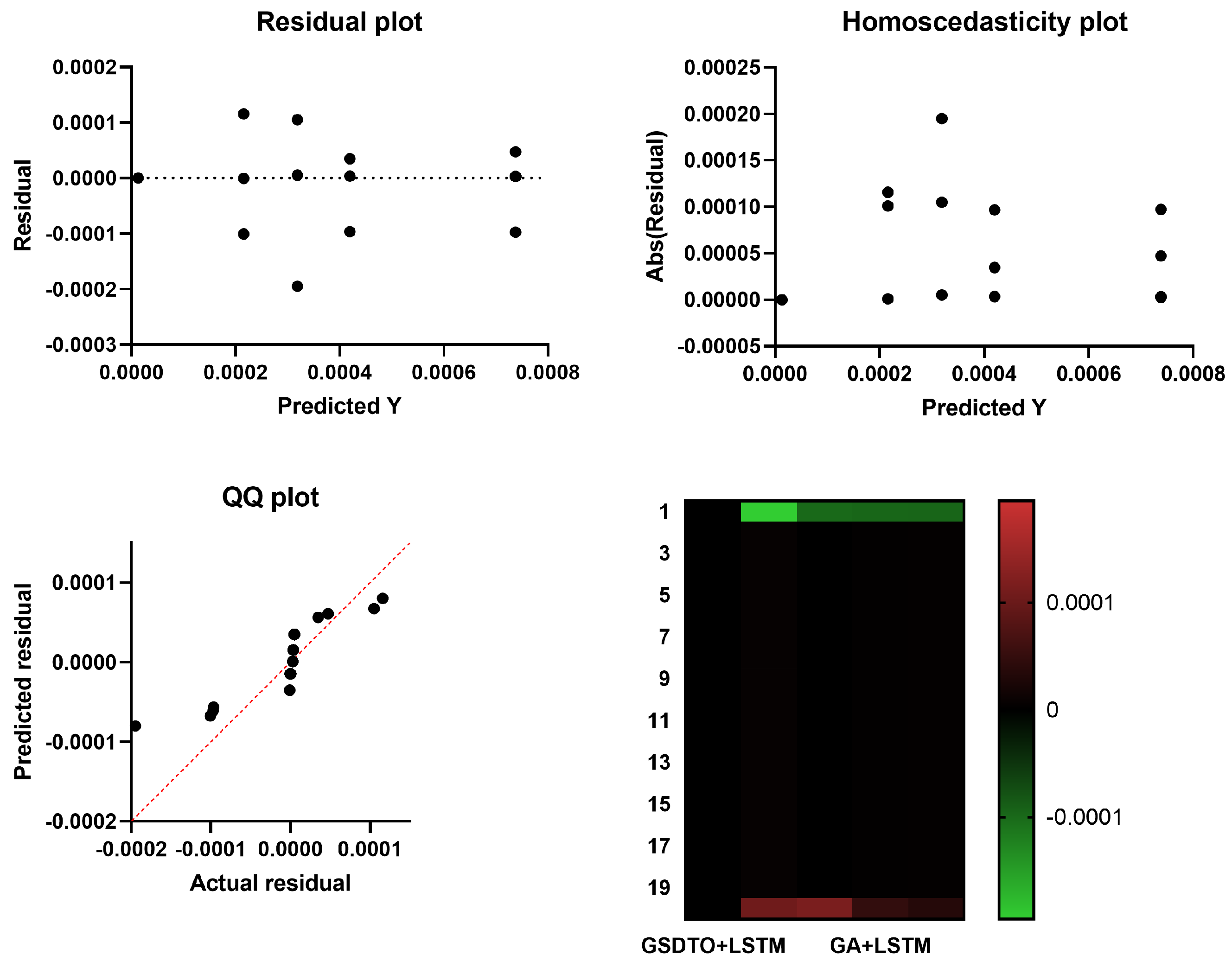
5.2. Regression Analysis
5.3. Statistical Significance
6. Conclusions and Future Work
Author Contributions
Funding
Institutional Review Board Statement
Informed Consent Statement
Data Availability Statement
Acknowledgments
Conflicts of Interest
References
- Badawi, M.; Ibrahim, S.A.; Mansour, D.E.A.; El-Faraskoury, A.A.; Ward, S.A.; Mahmoud, K.; Lehtonen, M.; Darwish, M.M.F. Reliable Estimation for Health Index of Transformer Oil Based on Novel Combined Predictive Maintenance Techniques. IEEE Access 2022, 10, 25954–25972. [Google Scholar] [CrossRef]
- Ghoneim, S.S.M.; Farrag, T.A.; Rashed, A.A.; El-Kenawy, E.S.M.; Ibrahim, A. Adaptive Dynamic Meta-Heuristics for Feature Selection and Classification in Diagnostic Accuracy of Transformer Faults. IEEE Access 2021, 9, 78324–78340. [Google Scholar] [CrossRef]
- Gouda, O.E.; El-Hoshy, S.H.; El-Tamaly, H.H. Proposed heptagon graph for DGA interpretation of oil transformers. IET Gener. Transm. Distrib. 2018, 12, 490–498. [Google Scholar] [CrossRef]
- Ward, S.A.; El-Faraskoury, A.; Badawi, M.; Ibrahim, S.A.; Mahmoud, K.; Lehtonen, M.; Darwish, M.M.F. Towards Precise Interpretation of Oil Transformers via Novel Combined Techniques Based on DGA and Partial Discharge Sensors. Sensors 2021, 21, 2223. [Google Scholar] [CrossRef]
- Benmahamed, Y.; Kherif, O.; Teguar, M.; Boubakeur, A.; Ghoneim, S.S.M. Accuracy Improvement of Transformer Faults Diagnostic Based on DGA Data Using SVM-BA Classifier. Energies 2021, 14, 2970. [Google Scholar] [CrossRef]
- Std C57.104-2008; IEEE Guide for the Interpretation of Gases Generated in Oil-Immersed Transformers. IEEE: Piscataway, NJ, USA, 2009; pp. 1–36. [CrossRef]
- IEC 60599: Mineral Oil-Filled Electrical Equipment in Service—Guidance on the Interpretation of Dissolved and Free Gases Analysis, Edition 2.1; IEC: Geneva, Switzerland, 2007.
- Duval, M. A review of faults detectable by gas-in-oil analysis in transformers. IEEE Electr. Insul. Mag. 2002, 18, 8–17. [Google Scholar] [CrossRef]
- Duval, M.; dePabla, A. Interpretation of gas-in-oil analysis using new IEC publication 60599 and IEC TC 10 databases. IEEE Electr. Insul. Mag. 2001, 17, 31–41. [Google Scholar] [CrossRef]
- Gouda, O.E.; El-Hoshy, S.H.; Ghoneim, S.S.M. Enhancing the Diagnostic Accuracy of DGA Techniques Based on IEC-TC10 and Related Databases. IEEE Access 2021, 9, 118031–118041. [Google Scholar] [CrossRef]
- Faiz, J.; Soleimani, M. Assessment of computational intelligence and conventional dissolved gas analysis methods for transformer fault diagnosis. IEEE Trans. Dielectr. Electr. Insul. 2018, 25, 1798–1806. [Google Scholar] [CrossRef]
- Hoballah, A.; Mansour, D.E.A.; Taha, I.B.M. Hybrid Grey Wolf Optimizer for Transformer Fault Diagnosis Using Dissolved Gases Considering Uncertainty in Measurements. IEEE Access 2020, 8, 139176–139187. [Google Scholar] [CrossRef]
- Li, X.; Wu, H.; Wu, D. DGA Interpretation Scheme Derived From Case Study. IEEE Trans. Power Deliv. 2011, 26, 1292–1293. [Google Scholar] [CrossRef]
- The duval pentagon-a new complementary tool for the interpretation of dissolved gas analysis in transformers. IEEE Electr. Insul. Mag. 2014, 30, 9–12. [CrossRef]
- Cheim, L.; Duval, M.; Haider, S. Combined Duval Pentagons: A Simplified Approach. Energies 2020, 13, 2859. [Google Scholar] [CrossRef]
- Mansour, D.E.A. Development of a new graphical technique for dissolved gas analysis in power transformers based on the five combustible gases. IEEE Trans. Dielectr. Electr. Insul. 2015, 22, 2507–2512. [Google Scholar] [CrossRef]
- Miranda, V.; Castro, A. Improving the IEC Table for Transformer Failure Diagnosis with Knowledge Extraction from Neural Networks. IEEE Trans. Power Deliv. 2005, 20, 2509–2516. [Google Scholar] [CrossRef]
- Souahlia, S.; Bacha, K.; Chaari, A. MLP neural network-based decision for power transformers fault diagnosis using an improved combination of Rogers and Doernenburg ratios DGA. Int. J. Electr. Power Energy Syst. 2012, 43, 1346–1353. [Google Scholar] [CrossRef]
- Guardado, J.; Naredo, J.; Moreno, P.; Fuerte, C. A comparative study of neural network efficiency in power transformers diagnosis using dissolved gas analysis. IEEE Trans. Power Deliv. 2001, 16, 643–647. [Google Scholar] [CrossRef]
- Equbal, M.D.; Khan, S.A.; Islam, T. Transformer incipient fault diagnosis on the basis of energy-weighted DGA using an artificial neural network. Turk. J. Electr. Eng. Comput. Sci. 2018, 26, 77–88. [Google Scholar] [CrossRef]
- Ou, M.; Wei, H.; Zhang, Y.; Tan, J. A Dynamic Adam Based Deep Neural Network for Fault Diagnosis of Oil-Immersed Power Transformers. Energies 2019, 12, 995. [Google Scholar] [CrossRef] [Green Version]
- Abu-Siada, A.; Hmood, S.; Islam, S. A new fuzzy logic approach for consistent interpretation of dissolved gas-in-oil analysis. IEEE Trans. Dielectr. Electr. Insul. 2013, 20, 2343–2349. [Google Scholar] [CrossRef]
- Noori, M.; Effatnejad, R.; Hajihosseini, P. Using dissolved gas analysis results to detect and isolate the internal faults of power transformers by applying a fuzzy logic method. IET Gener. Transm. Distrib. 2017, 11, 2721–2729. [Google Scholar] [CrossRef]
- Mulyodinoto, K.U.; Prasojo, R.A.; Abu-Siada, A. Applications of ANFIS to Estimate the Degree of Polymerization Using Transformer Dissolve Gas Analysis and Oil Characteristics. Polym. Sci. 2018, 14, 1–9. [Google Scholar]
- Bacha, K.; Souahlia, S.; Gossa, M. Power transformer fault diagnosis based on dissolved gas analysis by support vector machine. Electr. Power Syst. Res. 2012, 83, 73–79. [Google Scholar] [CrossRef]
- Zhang, Y.; Li, X.; Zheng, H.; Yao, H.; Liu, J.; Zhang, C.; Peng, H.; Jiao, J. A Fault Diagnosis Model of Power Transformers Based on Dissolved Gas Analysis Features Selection and Improved Krill Herd Algorithm Optimized Support Vector Machine. IEEE Access 2019, 7, 102803–102811. [Google Scholar] [CrossRef]
- Taha, I.B.M.; Hoballah, A.; Ghoneim, S.S.M. Optimal ratio limits of rogers’ four-ratios and IEC 60599 code methods using particle swarm optimization fuzzy-logic approach. IEEE Trans. Dielectr. Electr. Insul. 2020, 27, 222–230. [Google Scholar] [CrossRef]
- Illias, H.A.; Chai, X.R.; Bakar, A.H.A.; Mokhlis, H. Transformer Incipient Fault Prediction Using Combined Artificial Neural Network and Various Particle Swarm Optimisation Techniques. PLoS ONE 2015, 10, e0129363. [Google Scholar] [CrossRef]
- Illias, H.A.; Chai, X.R.; Bakar, A.H.A. Hybrid modified evolutionary particle swarm optimisation-time varying acceleration coefficient-artificial neural network for power transformer fault diagnosis. Measurement 2016, 90, 94–102. [Google Scholar] [CrossRef]
- Ghoneim, S.S.M.; Mahmoud, K.; Lehtonen, M.; Darwish, M.M.F. Enhancing Diagnostic Accuracy of Transformer Faults Using Teaching-Learning-Based Optimization. IEEE Access 2021, 9, 30817–30832. [Google Scholar] [CrossRef]
- Bello, R.; Gomez, Y.; Nowe, A.; Garcia, M.M. Two-Step Particle Swarm Optimization to Solve the Feature Selection Problem. In Proceedings of the Seventh International Conference on Intelligent Systems Design and Applications (ISDA 2007), Rio de Janeiro, Brazil, 20–24 October 2007; pp. 691–696. [Google Scholar] [CrossRef]
- El-Kenawy, E.S.M.; Eid, M.M.; Saber, M.; Ibrahim, A. MbGWO-SFS: Modified Binary Grey Wolf Optimizer Based on Stochastic Fractal Search for Feature Selection. IEEE Access 2020, 8, 107635–107649. [Google Scholar] [CrossRef]
- Eid, M.M.; El-kenawy, E.S.M.; Ibrahim, A. A binary Sine Cosine-Modified Whale Optimization Algorithm for Feature Selection. In Proceedings of the 2021 National Computing Colleges Conference (NCCC), Taif, Saudi Arabia, 27–28 March 2021. [Google Scholar] [CrossRef]
- Simon, D. Biogeography-Based Optimization. IEEE Trans. Evol. Comput. 2008, 12, 702–713. [Google Scholar] [CrossRef]
- Fister, I.; Yang, X.S.; Fister, I.; Brest, J. Memetic Firefly Algorithm for Combinatorial Optimization. arXiv 2012, arXiv:1204.5165. [Google Scholar]
- Kabir, M.M.; Shahjahan, M.; Murase, K. A new local search based hybrid genetic algorithm for feature selection. Neurocomputing 2011, 74, 2914–2928. [Google Scholar] [CrossRef]
- Karakonstantis, I.; Vlachos, A. Bat algorithm applied to continuous constrained optimization problems. J. Inf. Optim. Sci. 2021, 42, 57–75. [Google Scholar] [CrossRef]
- Egyptian Electricity Holding Company (EEHC) Reports. Available online: http://www.moee.gov.eg/english_new/report.aspx (accessed on 18 April 2022).
- Agrawal, S.; Chandel, A.K. Transformer incipient fault diagnosis based on probabilistic neural network. In Proceedings of the 2012 Students Conference on Engineering and Systems, Allahabad, India, 16–18 March 2012; IEEE: Piscataway, NJ, USA, 2012. [Google Scholar] [CrossRef]
- Wang, M.H. A novel extension method for transformer fault diagnosis. IEEE Trans. Power Deliv. 2003, 18, 164–169. [Google Scholar] [CrossRef]
- Zhu, Y.; Wang, F.; Geng, L. Transformer Fault Diagnosis Based on Naive Bayesian Classifier and SVR. In Proceedings of the TENCON 2006–2006 IEEE Region 10 Conference, Hong Kong, China, 14–17 November 2006; IEEE: Piscataway, NJ, USA, 2006. [Google Scholar] [CrossRef]
- Siva Sarma, D.V.S.S.; Kalyani, G.N.S. ANN approach for condition monitoring of power transformers using DGA. In Proceedings of the 2004 IEEE Region 10 Conference TENCON 2004, Chiang Mai, Thailand, 24 November 2004; Volume 3, pp. 444–447. [Google Scholar] [CrossRef]
- Hu, J.; Zhou, L.; Song, M. Transformer Fault Diagnosis Method of Gas Hromatographic Analysis Using Computer Image Analysis. In Proceedings of the 2012 Second International Conference on Intelligent System Design and Engineering Application, Sanya, China, 6–7 January 2012; pp. 1169–1172. [Google Scholar] [CrossRef]
- Seifeddine, S.; Khmais, B.; Abdelkader, C. Power transformer fault diagnosis based on dissolved gas analysis by artificial neural network. In Proceedings of the 2012 First International Conference on Renewable Energies and Vehicular Technology, Nabeul, Tunisia, 26–28 March 2012; pp. 230–236. [Google Scholar] [CrossRef]
- Rajabimendi, M.; Dadios, E.P. A hybrid algorithm based on neural-fuzzy system for interpretation of dissolved gas analysis in power transformers. In Proceedings of the TENCON 2012 IEEE Region 10 Conference, Cebu, Philippines, 19–22 November 2012; pp. 1–6. [Google Scholar] [CrossRef]
- Zhang, G.; Yasuoka, K.; Ishii, S.; Yang, L.; Yan, Z. Application of fuzzy equivalent matrix for fault diagnosis of oil-immersed insulation. In Proceedings of the 1999 IEEE 13th International Conference on Dielectric Liquids (ICDL’99) (Cat. No. 99CH36213), Nara, Japan, 25 July 1999; pp. 400–403. [CrossRef]
- Gouda, O.E.; Saleh, S.M.; El-hoshy, S.H. Power Transformer Incipient Faults Diagnosis Based on Dissolved Gas Analysis. Indones. J. Electr. Eng. Comput. Sci. 2016, 17, 10–16. [Google Scholar] [CrossRef]
- El-Kenawy, E.S.M.; Mirjalili, S.; Ibrahim, A.; Alrahmawy, M.; El-Said, M.; Zaki, R.M.; Eid, M.M. Advanced Meta-Heuristics, Convolutional Neural Networks, and Feature Selectors for Efficient COVID-19 X-Ray Chest Image Classification. IEEE Access 2021, 9, 36019–36037. [Google Scholar] [CrossRef]
- Ibrahim, A.; Mirjalili, S.; El-Said, M.; Ghoneim, S.S.M.; Al-Harthi, M.M.; Ibrahim, T.F.; El-Kenawy, E.S.M. Wind Speed Ensemble Forecasting Based on Deep Learning Using Adaptive Dynamic Optimization Algorithm. IEEE Access 2021, 9, 125787–125804. [Google Scholar] [CrossRef]
- Takieldeen, A.E.; El-kenawy, E.S.M.; Hadwan, M.; Zaki, R.M. Dipper Throated Optimization Algorithm for Unconstrained Function and Feature Selection. Comput. Mater. Contin. 2022, 72, 1465–1481. [Google Scholar] [CrossRef]
- El-kenawy, E.S.M.; Mirjalili, S.; Ghoneim, S.S.M.; Eid, M.M.; El-Said, M.; Khan, Z.S.; Ibrahim, A. Advanced Ensemble Model for Solar Radiation Forecasting using Sine Cosine Algorithm and Newton’s Laws. IEEE Access 2021, 9, 115750–115765. [Google Scholar] [CrossRef]
- Emary, E.; Zawbaa, H.M.; Hassanien, A.E. Binary grey wolf optimization approaches for feature selection. Neurocomputing 2016, 172, 371–381. [Google Scholar] [CrossRef]
- Taha, I.B.; Dessouky, S.S.; Ghoneim, S.S. Transformer fault types and severity class prediction based on neural pattern-recognition techniques. Electr. Power Syst. Res. 2021, 191, 106899. [Google Scholar] [CrossRef]
- Confalonieri, R.; Bellocchi, G.; Bregaglio, S.; Donatelli, M.; Acutis, M. Comparison of sensitivity analysis techniques: A case study with the rice model WARM. Ecol. Model. 2010, 221, 1897–1906. [Google Scholar] [CrossRef]


| Ref. | PD | D1 | D2 | T1 | T2 | T3 | Total |
|---|---|---|---|---|---|---|---|
| [8] | 2 | 0 | 0 | 3 | 0 | 0 | 5 |
| [9] | 9 | 24 | 48 | 0 | 0 | 18 | 99 |
| [25] | 0 | 2 | 1 | 1 | 3 | 1 | 8 |
| [38] | 27 | 42 | 55 | 70 | 18 | 28 | 240 |
| [39] | 1 | 0 | 5 | 2 | 0 | 1 | 9 |
| [40] | 3 | 0 | 4 | 4 | 3 | 5 | 19 |
| [41] | 1 | 1 | 2 | 1 | 0 | 1 | 6 |
| Total | 43 | 69 | 115 | 81 | 24 | 54 | 386 |
| Ref. | PD | D1 | D2 | T1 | T2 | T3 | Total |
|---|---|---|---|---|---|---|---|
| [9] | 1 | 6 | 8 | 1 | 1 | 17 | |
| [38] | 6 | 6 | 11 | 11 | 3 | 2 | 39 |
| [40] | 2 | 1 | 3 | ||||
| [41] | 1 | 1 | |||||
| [42] | 2 | 2 | |||||
| [43] | 1 | 1 | |||||
| [44] | 1 | 1 | 1 | 3 | |||
| [45] | 1 | 1 | |||||
| [46] | 2 | 1 | 3 | 6 | |||
| [47] | 1 | 1 | |||||
| Total | 7 | 13 | 24 | 16 | 4 | 10 | 74 |
| Parameter (s) | Value (s) |
|---|---|
| # Agents | 10 |
| # Iterations | 80 |
| # Repetitions | 20 |
| Dimension | # features |
| C | |
| R | |
| of | 0.99 |
| of | 0.01 |
| Algorithm | Parameter (s) | Value (s) |
|---|---|---|
| PSO | , | [0.9, 0.6] |
| , | [2, 2] | |
| GWO | a | 2 to 0 |
| WOA | a | 2 to 0 |
| r | [0, 1] | |
| BBO | Habitat modification Probability | 1.0 |
| Mutation Probability | 0.05 | |
| Immigration Probability | [0, 1] | |
| Migration rate | 1.0 | |
| Max immigration | 1.0 | |
| Step size | 1.0 | |
| BA | Pluse rate | 0.5 |
| Loudness | 0.5 | |
| Frequency | [0, 1] | |
| GA | Crossover | 0.9 |
| Mutation ratio | 0.1 | |
| Mechanism of Selection | Roulette wheel | |
| FA | # Fireflies | 10 |
| Metric | Value |
|---|---|
| Average Error | |
| Average Select Size | |
| Average Fitness | |
| Best Fitness | |
| Worst Fitness | |
| Standard Deviation |
| bGSDTO | bGWO | bPSO | bBA | bWOA | bBBO | bFA | bGA | |
|---|---|---|---|---|---|---|---|---|
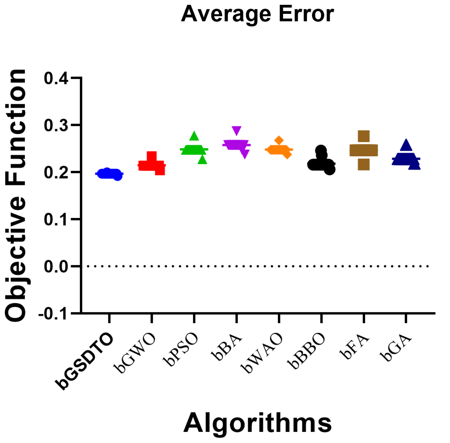
| Average error | 0.1969 | 0.2141 | 0.2479 | 0.2575 | 0.2477 | 0.2161 | 0.2463 | 0.2277 |
| Average Select size | 0.1497 | 0.3497 | 0.3497 | 0.4891 | 0.5131 | 0.5135 | 0.3842 | 0.2921 |
| Average Fitness | 0.2601 | 0.2763 | 0.2747 | 0.2976 | 0.2825 | 0.2804 | 0.3266 | 0.2877 |
| Best Fitness | 0.1619 | 0.1966 | 0.255 | 0.1873 | 0.2466 | 0.2701 | 0.2453 | 0.191 |
| Worst Fitness | 0.2604 | 0.2635 | 0.3227 | 0.2889 | 0.3227 | 0.3566 | 0.3429 | 0.3061 |
| Standard deviation Fitness | 0.0824 | 0.0871 | 0.0865 | 0.0964 | 0.0887 | 0.1314 | 0.1233 | 0.0887 |
| SS | DF | MS | F (DFn, DFd) | p Value | |
|---|---|---|---|---|---|
| Treatment (between columns) | 0.06262 | 7 | 0.008946 | F (7, 152) = 173.9 | p < 0.0001 |
| Residual (within columns) | 0.007819 | 152 | 0.00005144 | - | - |
| Total | 0.07044 | 159 | - | - | - |
| bGSDTO | bGWO | bPSO | bBA | bWOA | bBBO | bFA | bGA | |
|---|---|---|---|---|---|---|---|---|
| Theoretical median | 0 | 0 | 0 | 0 | 0 | 0 | 0 | 0 |
| Actual median | 0.1969 | 0.2141 | 0.2479 | 0.2575 | 0.2477 | 0.2161 | 0.2463 | 0.2277 |
| # Values | 20 | 20 | 20 | 20 | 20 | 20 | 20 | 20 |
| Wilcoxon Signed Rank Test | ||||||||
| Signed ranks’ sum | 210 | 210 | 210 | 210 | 210 | 210 | 210 | 210 |
| Positive ranks’ sum | 210 | 210 | 210 | 210 | 210 | 210 | 210 | 210 |
| Negative ranks’ sum | 0 | 0 | 0 | 0 | 0 | 0 | 0 | 0 |
| P value (two tailed) | <0.0001 | <0.0001 | <0.0001 | <0.0001 | <0.0001 | <0.0001 | <0.0001 | <0.0001 |
| Exact or estimate? | Exact | Exact | Exact | Exact | Exact | Exact | Exact | Exact |
| Significant (alpha = 0.05)? | Yes | Yes | Yes | Yes | Yes | Yes | Yes | Yes |
| Discrepancy | 0.1969 | 0.2141 | 0.2479 | 0.2575 | 0.2477 | 0.2161 | 0.2463 | 0.2277 |
| Classifier | Parameter (s) | Value (s) |
|---|---|---|
| NN | beta_1 | 0.6 |
| beta_2 | 0.899 | |
| epsilon | 1 × 10 | |
| validation_fraction | 0.1 | |
| learning_rate_init | 0.007 | |
| hidden_layer_sizes | 20 | |
| k-NN | leaf_size | 20 |
| p | 2 | |
| n_neighbors | 3 | |
| RF | min_weight_fraction_leaf | 0.0 |
| min_samples_leaf | 1 | |
| n_estimators | 40 | |
| min_samples_split | 2 |
| Model | AUC | MSE |
|---|---|---|
| NN | 0.744 | 0.080226 |
| K-NN | 0.7387 | 0.098999 |
| RF | 0.797 | 0.04887 |
| GSDTO+LSTM | WOA+LSTM | GWO+LSTM | GA+LSTM | PSO+LSTM | |
|---|---|---|---|---|---|
| AUC | 0.9826 | 0.957 | 0.943 | 0.934 | 0.949 |
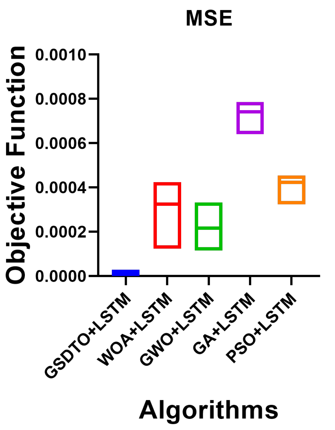
| MSE | 0.00001413 | 0.000319 | 0.0002158 | 0.0007382 | 0.0004196 |
| GSDTO+LSTM | WOA+LSTM | GWO+LSTM | GA+LSTM | PSO+LSTM | |
|---|---|---|---|---|---|
| Number of values | 20 | 20 | 20 | 20 | 20 |
| Minimum | 0.0000133 | 0.000124 | 0.000115 | 0.000641 | 0.000323 |
| 25% Percentile | 0.0000133 | 0.000324 | 0.000215 | 0.000741 | 0.000423 |
| Median | 0.0000133 | 0.000324 | 0.000215 | 0.000741 | 0.000423 |
| 75% Percentile | 0.0000133 | 0.000324 | 0.000215 | 0.000741 | 0.000423 |
| Maximum | 0.0000133 | 0.000424 | 0.0003315 | 0.0007854 | 0.000454 |
| Range | 0 | 0.0003 | 0.0002165 | 0.0001444 | 0.000131 |
| 10% Percentile | 0.0000133 | 0.000324 | 0.000215 | 0.000741 | 0.000423 |
| 90% Percentile | 0.0000133 | 0.000324 | 0.000215 | 0.000741 | 0.000423 |
| Mean | 0.0000133 | 0.000319 | 0.0002158 | 0.0007382 | 0.00042 |
| Std. Deviation | 0 | 0.00005104 | 0.00003521 | ||
| Std. Error of Mean | 0 | 0.00001141 | |||
| Coefficient of variation | 0.000% | 16.00% | 16.32% | 3.378% | 5.666% |
| Geometric mean | 0.0000133 | 0.000313 | 0.0002129 | 0.0007378 | 0.000419 |
| Geometric SD factor | 1 | 1.254 | 1.19 | 1.036 | 1.065 |
| Harmonic mean | 0.0000133 | 0.0003031 | 0.0002096 | 0.0007373 | 0.000418 |
| Quadratic mean | 0.0000133 | 0.0003229 | 0.0002185 | 0.0007386 | 0.00042 |
| Skewness | −2.751 | 0.7003 | −3.067 | −3.734 | |
| Kurtosis | 13.14 | 9.729 | 14.07 | 16.45 | |
| Sum | 0.000266 | 0.00638 | 0.004317 | 0.01476 | 0.008391 |
| GSDTO+LSTM | WOA+LSTM | GWO+LSTM | GA+LSTM | PSO+LSTM | |
|---|---|---|---|---|---|
| Theoretical median | 0 | 0 | 0 | 0 | 0 |
| Actual median | 0.0000133 | 0.000324 | 0.000215 | 0.000741 | 0.000423 |
| # values | 20 | 20 | 20 | 20 | 20 |
| Wilcoxon Signed-Rank | |||||
| Signed ranks’ Sum (W) | 210 | 210 | 210 | 210 | 210 |
| Positive ranks’ Sum | 210 | 210 | 210 | 210 | 210 |
| Negative ranks’ Sum | 0 | 0 | 0 | 0 | 0 |
| P value (two tailed) | <0.0001 | <0.0001 | <0.0001 | <0.0001 | <0.0001 |
| Estimate or Exact? | Exact | Exact | Exact | Exact | Exact |
| Significant ()? | Yes | Yes | Yes | Yes | Yes |
| How big is the discrepancy? | |||||
| Discrepancy | 0.0000133 | 0.000324 | 0.000215 | 0.000741 | 0.000423 |
| Fault Type | Samples | GSDTO+LSTM | Adaptive [2] | IEC-60599 [7] | IEC 60599 Modified [27] | Rog. Modified [27] |
| PD | 7 | 100 | 100 | 28.57 | 100 | 100 |
| D1 | 13 | 100 | 92.31 | 30.77 | 61.54 | 61.54 |
| D2 | 24 | 95.83 | 91.67 | 41.67 | 87.5 | 79.17 |
| T1 | 16 | 93.75 | 93.95 | 68.75 | 100 | 100 |
| T2 | 4 | 100 | 100 | 75 | 100 | 100 |
| T3 | 10 | 100 | 100 | 70 | 100 | 100 |
| Overall | 74 | 98.26 | 94.6 | 50 | 89.19 | 86.49 |
| Fault Type | Samples | Duval [8,9] | NPR [53] | SVM [53] | Rog. 4 Ratios [6] | |
| PD | 7 | 42.86 | 100 | 85.71 | 14.29 | |
| D1 | 13 | 69.23 | 76.92 | 76.92 | 0 | |
| D2 | 24 | 75 | 87.5 | 91.67 | 50 | |
| T1 | 16 | 56.25 | 100 | 100 | 100 | |
| T2 | 4 | 0 | 75 | 25 | 25 | |
| T3 | 10 | 100 | 100 | 100 | 40 | |
| Overall | 74 | 66.27 | 90.54 | 87.84 | 45.95 |
| R-Parameter | Exploration Percentage | Population Size | Iterations Count | C-Parameter | |||||
|---|---|---|---|---|---|---|---|---|---|
| Values | Time | Values | Time | Values | Time | Values | Time | Values | Time |
| 0.05 | 3.353 | 5 | 3.257 | 10 | 0.5 | 10 | 0.662 | 0.1 | 3.371 |
| 0.1 | 3.145 | 10 | 3.717 | 20 | 1.523 | 20 | 0.244 | 0.2 | 3.328 |
| 0.15 | 3.018 | 15 | 3.442 | 30 | 3.095 | 30 | 1.146 | 0.3 | 3.262 |
| 0.2 | 3.503 | 20 | 3.249 | 40 | 4.933 | 40 | 2.038 | 0.4 | 3.246 |
| 0.25 | 3.251 | 25 | 3.048 | 50 | 6.28 | 50 | 2.935 | 0.5 | 3.302 |
| 0.3 | 3.114 | 30 | 3.049 | 60 | 7.704 | 60 | 3.848 | 0.6 | 3.259 |
| 0.35 | 3.071 | 35 | 3.044 | 70 | 9.253 | 70 | 4.786 | 0.7 | 3.289 |
| 0.4 | 3.06 | 40 | 3.081 | 80 | 10.817 | 80 | 6.649 | 0.8 | 3.22 |
| 0.45 | 3.037 | 45 | 3.039 | 90 | 12.324 | 90 | 7.463 | 0.9 | 3.285 |
| 0.5 | 3.041 | 50 | 3.039 | 100 | 13.881 | 100 | 10.226 | 1 | 3.304 |
| 0.55 | 3.028 | 55 | 3.059 | 110 | 15.439 | 110 | 11.123 | 1.1 | 3.259 |
| 0.6 | 3.037 | 60 | 3.067 | 120 | 17.962 | 120 | 11.995 | 1.2 | 3.208 |
| 0.65 | 3.129 | 65 | 3.058 | 130 | 19.292 | 130 | 13.011 | 1.3 | 3.278 |
| 0.7 | 6.341 | 70 | 3.034 | 140 | 20.21 | 140 | 13.798 | 1.4 | 3.277 |
| 0.75 | 6.272 | 75 | 3.041 | 150 | 21.582 | 150 | 15.892 | 1.5 | 3.226 |
| 0.8 | 6.082 | 80 | 3.048 | 160 | 23.173 | 160 | 16.864 | 1.6 | 3.213 |
| 0.85 | 4.279 | 85 | 3.042 | 170 | 25.767 | 170 | 17.083 | 1.7 | 3.218 |
| 0.9 | 4.57 | 90 | 3.06 | 180 | 30.937 | 180 | 17.872 | 1.8 | 3.211 |
| 0.95 | 3.34 | 95 | 3.058 | 190 | 35.502 | 190 | 19.415 | 1.9 | 3.195 |
| 1 | 3.794 | 95 | 3.042 | 200 | 35.077 | 200 | 20.267 | 2 | 3.186 |
| R-Parameter | Exploration Percentage | Population Size | Iterations Count | C-Parameter | |||||
|---|---|---|---|---|---|---|---|---|---|
| Values | Fitness | Values | Fitness | Values | Fitness | Values | Fitness | Values | Fitness |
| 0.05 | −11.2816 | 5 | −9.1386 | 10 | −9.6506 | 50 | −7.5286 | 0.1 | −8.0656 |
| 0.1 | −11.2816 | 10 | −9.1376 | 20 | −12.3506 | 100 | −6.9926 | 0.2 | −8.0656 |
| 0.15 | −11.8186 | 15 | −11.2846 | 30 | −11.2826 | 150 | −8.6006 | 0.3 | −6.9926 |
| 0.2 | −11.8206 | 20 | −10.7486 | 40 | −11.2856 | 200 | −8.6026 | 0.4 | −8.0626 |
| 0.25 | −11.2836 | 25 | −11.2806 | 50 | −10.2126 | 250 | −8.0656 | 0.5 | −8.0656 |
| 0.3 | −11.2846 | 30 | −10.7486 | 60 | −12.3586 | 300 | −8.0656 | 0.6 | −6.9926 |
| 0.35 | −10.7476 | 35 | −10.7486 | 70 | −12.3586 | 350 | −9.6756 | 0.7 | −8.0656 |
| 0.4 | −11.2856 | 40 | −11.2856 | 80 | −12.3586 | 450 | −8.0656 | 0.8 | −8.0616 |
| 0.45 | −10.7486 | 45 | −11.2846 | 90 | −11.8226 | 500 | −9.1386 | 0.9 | −6.9926 |
| 0.5 | −11.2846 | 50 | −10.2126 | 100 | −12.3586 | 650 | −10.2126 | 1 | −8.0656 |
| 0.55 | −11.2846 | 55 | −11.2856 | 110 | −12.3586 | 700 | −8.6026 | 1.1 | −8.0656 |
| 0.6 | −12.3556 | 60 | −11.8206 | 120 | −12.3586 | 750 | −10.2126 | 1.2 | −8.0656 |
| 0.65 | −11.2846 | 65 | −11.2836 | 130 | −12.3586 | 800 | −10.7486 | 1.3 | −9.1386 |
| 0.7 | −10.7476 | 70 | −11.2846 | 140 | −12.3586 | 850 | −9.1386 | 1.4 | −10.2116 |
| 0.75 | −10.7466 | 75 | −11.2856 | 150 | −12.3586 | 900 | −9.6756 | 1.5 | −11.2836 |
| 0.8 | −12.3546 | 80 | −10.7476 | 160 | −12.3586 | 950 | −10.7486 | 1.6 | −9.1386 |
| 0.85 | −11.2366 | 85 | −12.3556 | 170 | −12.3586 | 1000 | −10.2126 | 1.7 | −10.2116 |
| 0.9 | −11.8096 | 90 | −11.2716 | 180 | −12.3586 | 1050 | −10.7486 | 1.8 | −12.3576 |
| 0.95 | −12.3196 | 95 | −11.2746 | 190 | −12.3586 | 1150 | −9.6756 | 1.9 | −11.2846 |
| 1 | −12.3306 | 95 | −11.8096 | 200 | −12.3586 | 1200 | −10.2126 | 2 | −12.3586 |
| Convergence Time | Minimum Fitness | |||
|---|---|---|---|---|
| Parameters | R Square | Significance F | R Square | Significance F |
| R-Parameter | ||||
| Exploration Percentage | ||||
| Population Size | ||||
| Iterations Count | ||||
| C-Parameter | ||||
| SS | DF | MS | F (DFn, DFd) | p Value | |
|---|---|---|---|---|---|
| Treatment (between columns) | 11.54 | 9 | 1.282 | F (9, 190) = 2483 | p < 0.0001 |
| Residual (within columns) | 0.0981 | 190 | 0.0005163 | - | - |
| Total | 11.64 | 199 | - | - | - |
| Convergence Time | |||||
| R-Parameter | Exploration Percentage | Population Size | Iterations Count | C-Parameter | |
| Theoretical mean | 0 | 0 | 0 | 0 | 0 |
| Actual mean | 0.7775 | 0.593 | 0.8025 | 0.828 | 0.421 |
| Number of values | 20 | 20 | 20 | 20 | 20 |
| One sample t test | |||||
| t, df | t = 93.03, df = 19 | t = 48.00, df = 19 | t = 72.62, df = 19 | t = 93.97, df = 19 | t = 38.47, df = 19 |
| p value (two tailed) | <0.0001 | <0.0001 | <0.0001 | <0.0001 | <0.0001 |
| p value summary | **** | **** | **** | **** | **** |
| Significant (alpha = 0.05)? | Yes | Yes | Yes | Yes | Yes |
| How big is the discrepancy? | |||||
| Discrepancy | 0.7775 | 0.593 | 0.8025 | 0.828 | 0.421 |
| SD of discrepancy | 0.03738 | 0.05525 | 0.04942 | 0.0394 | 0.04894 |
| SEM of discrepancy | 0.008357 | 0.01235 | 0.01105 | 0.008811 | 0.01094 |
| 95% confidence interval | 0.7600 to 0.7949 | 0.5671 to 0.6189 | 0.7794 to 0.8256 | 0.8096 to 0.8464 | 0.3981 to 0.4439 |
| R squared (partial eta squared) | 0.9978 | 0.9918 | 0.9964 | 0.9979 | 0.9873 |
| Minimum Fitness | |||||
| R-Parameter | Exploration Percentage | Population Size | Iterations Count | C-Parameter | |
| Theoretical mean | 0 | 0 | 0 | 0 | 0 |
| Actual mean | 0.885 | 0.6412 | 0.9764 | 0.759 | 0.937 |
| Number of values | 20 | 20 | 20 | 20 | 20 |
| One sample t test | |||||
| t, df | t = 122.0, df = 19 | t = 87.20, df = 19 | t = 188.8, df = 19 | t = 57.81, df = 19 | t = 80.10, df = 19 |
| p value (two tailed) | <0.0001 | <0.0001 | <0.0001 | <0.0001 | <0.0001 |
| p value summary | **** | **** | **** | **** | **** |
| Significant (alpha = 0.05)? | Yes | Yes | Yes | Yes | Yes |
| How big is the discrepancy? | |||||
| Discrepancy | 0.885 | 0.6412 | 0.9764 | 0.759 | 0.937 |
| SD of discrepancy | 0.03244 | 0.03289 | 0.02313 | 0.05871 | 0.05231 |
| SEM of discrepancy | 0.007255 | 0.007353 | 0.005172 | 0.01313 | 0.0117 |
| 95% confidence interval | 0.8698 to 0.9002 | 0.6258 to 0.6566 | 0.9656 to 0.9872 | 0.7315 to 0.7865 | 0.9125 to 0.9615 |
| R squared (partial eta squared) | 0.9987 | 0.9975 | 0.9995 | 0.9943 | 0.997 |
Publisher’s Note: MDPI stays neutral with regard to jurisdictional claims in published maps and institutional affiliations. |
© 2022 by the authors. Licensee MDPI, Basel, Switzerland. This article is an open access article distributed under the terms and conditions of the Creative Commons Attribution (CC BY) license (https://creativecommons.org/licenses/by/4.0/).
Share and Cite
El-kenawy, E.-S.M.; Albalawi, F.; Ward, S.A.; Ghoneim, S.S.M.; Eid, M.M.; Abdelhamid, A.A.; Bailek, N.; Ibrahim, A. Feature Selection and Classification of Transformer Faults Based on Novel Meta-Heuristic Algorithm. Mathematics 2022, 10, 3144. https://doi.org/10.3390/math10173144
El-kenawy E-SM, Albalawi F, Ward SA, Ghoneim SSM, Eid MM, Abdelhamid AA, Bailek N, Ibrahim A. Feature Selection and Classification of Transformer Faults Based on Novel Meta-Heuristic Algorithm. Mathematics. 2022; 10(17):3144. https://doi.org/10.3390/math10173144
Chicago/Turabian StyleEl-kenawy, El-Sayed M., Fahad Albalawi, Sayed A. Ward, Sherif S. M. Ghoneim, Marwa M. Eid, Abdelaziz A. Abdelhamid, Nadjem Bailek, and Abdelhameed Ibrahim. 2022. "Feature Selection and Classification of Transformer Faults Based on Novel Meta-Heuristic Algorithm" Mathematics 10, no. 17: 3144. https://doi.org/10.3390/math10173144