Fixed-Time Convergent Gradient Neural Network for Solving Online Sylvester Equation

Abstract

This paper aims at finding a fixed-time solution to the Sylvester equation by using a gradient neural network (GNN). To reach this goal, a modified sign-bi-power (msbp) function is presented and applied on a linear GNN as an activation function. Accordingly, a fixed-time convergent GNN (FTC-GNN) model is developed for solving the Sylvester equation. The upper bound of the convergence time of such an FTC-GNN model can be predetermined if parameters are given regardless of the initial conditions. This point is corroborated by a detailed theoretical analysis. In addition, the convergence time is also estimated utilizing the Lyapunov stability theory. Two examples are then simulated to demonstrate the validation of the theoretical analysis, as well as the superior convergence performance of the presented FTC-GNN model as compared to the existing GNN models.

1. Introduction

As a set of prominent and proverbial linear matrix equations, the Sylvester equation has aroused general concern among researchers in the past few decades, owing to its crucial role in matrix theory and diverse applications, such as image fusion [1], dimensionality reduction [2], linear descriptor systems [3], machine learning [4], the stabilization of PDE (partial differential equation)—ODE (ordinary differential equation) cascade systems [5], and so on. Consequently, a great deal of time and energy of researchers has been expended to put forward various numerical algorithms to rapidly seek out the solution to the Sylvester equation. Gradient-based iterative algorithms [6,7], the Bartels–Stewart algorithm [8], and its extensions [9,10] are some typical examples of them. Although the concrete forms of these algorithms may be diverse, they share one common characteristic, i.e., the solving process is carried out in a serial processing manner. In addition, generally speaking, $O\left(n^3\right)$ arithmetic operations are usually required to execute most of these numerical algorithms to seek out the solution [11,12]. It is thus predictable that vast amounts of time will be consumed (or, say, wasted) when applying these serial computational schemes to large-scale matrix-related problems (including the Sylvester equation), and it may be also inappropriate to apply them to real-time problem solving.

To work around these issues as well as to promote computational efficiency, parallel processing schemes based on recurrent neural networks (RNNs) are preferred and heralded as a powerful alternative. In addition to the characteristic of parallel processing, RNN models can be implemented expediently by circuit components in the wake of the rapid development of field-programmable gate array and integrated circuit technology [13,14,15]. As the result of these two outstanding features, a growing number of RNN models that aim at solving the Sylvester equation and related problems (e.g., matrix pseudoinverse) have been successively put forward and discussed in recent years [16,17,18,19,20,21,22,23,24,25]. ZNN (zeroing neural network) and GNN (gradient neural network) are two popular RNN categories that are extensively investigated in the literature. For example, in [16], by designing a matrix-valued error function and making use of the exponential decay formula, a novel RNN is proposed for finding the solution to the time-variant Sylvester equation. Following this groundbreaking work, a ZNN model under the action of the Li activation function (also termed the sign-bi-power function) is established for solving the time-variant Sylvester equation [17]. This model is the first ZNN model that realizes finite-time convergence. Inspired by this study, in [18], two nonlinear functions are exerted on linear ZNN as activation functions. Correspondingly, two predefined-time convergent ZNN models are successfully constructed for solving the time-variant Sylvester equation. Some ZNN models with varying design parameters are constructed and applied to the dynamic Sylvester equation and matrix pseudoinversion/inversion with real or complex coefficient matrices [19,20,21,22,23,24,25]. Additionally, discrete-time ZNN models based on continuous ZNN models are also developed for Sylvester equation solving [26,27,28,29].

On the other hand, a GNN model under the activation of four conventional functions is investigated in [30]. The property of global convergence of this GNN model is presented. To improve noise tolerance, a GNN model with an integration feedback term is proposed and investigated in [31]. In [32], a GNN model with adaptive coefficients is constructed to solve the time-varying Sylvester equation. To further quicken GNN models’ convergence speed, a sign-bi-power function activated GNN model that is able to converge to the theoretical solution of the Sylvester equation in finite time is established in [33]. Regrettably, the detailed theoretical analysis of this point and the estimate of the finite convergence time are not presented in the work. Recently, to solve the periodic Sylvester matrix equation, a GNN under the action of several activation functions is proposed and theoretically studied in [34].

It should be noted that, in more recent years, more efforts have focused on the development of finite-/fixed-time convergent ZNN models due to their superior convergence performance as compared to infinite-time convergent ZNN models. Comparatively, much fewer efforts are focused on the development and investigation of finite-time convergent GNN models. Moreover, in view of the fact that the convergence time of finite-time convergent GNN (and ZNN) models is heavily reliant on the initial state of the solving task, fixed-time convergent GNN models are much more preferable and imperatively needed. With these considerations, inspired by [35,36], a fast fixed-time convergent GNN (FTC-GNN) model is developed for solving the Sylvester equation in this paper. The resultant fixed-time convergent GNN model has a particular feature: the convergence time is bounded by a constant that is not bound up with the initial conditions.

We would like to emphasize the main contributions and novelties of this paper as follows.

(1)

As significant enhancements to the GNN models with infinite-time and finite-time convergence, a fixed-time convergent GNN (FTC-GNN) model is developed as a solution to the Sylvester equation. More specifically, the presented GNN model outperforms the linear GNN model [30] with exponential convergence (infinite-time convergence) and the sbp function activated GNN model [33] with declared finite-time convergence in terms of convergence performance.

(2)

The mathematical analysis of the fixed-time convergence of the presented GNN model is provided. It is shown that the convergence time of the presented FTC-GNN model has a predetermined upper bound, which is independent of the initial conditions. It is noted that infinite-time convergent (e.g., exponential convergence) and finite-time convergent GNN models do not have such a feature. In addition, the theoretical analysis in terms of convergence of the sbp function activated GNN model presented in the previous work [33] is also provided. These theoretical results demonstrate that the sbp function activated GNN model with declared finite-time convergence is, in fact, of fixed-time convergence, and the presented GNN model has faster fixed-time convergence as compared to the sbp function activated GNN model.

(3)

Comparative simulation results of two examples demonstrate the theoretical results as well as the superior convergence performance of the presented FTC-GNN model.

The remainder of this paper is structured as follows. Related preliminaries and some existing GNN models aimed at solving the Sylvester equation are presented in Section 2. In this section, for comparison and better illustration, a novel GNN model with fixed-time convergence is also established. The mathematical deduction on the fixed-time convergence of the presented GNN models is shown in Section 3. Section 4 presents two illustrative examples to demonstrate the theoretical results and the advantages of the presented FTC-GNN model over the existing GNN models in terms of convergence. Some remarks are given in Section 5.

2. Preliminaries and Model Description

In this section, the related preliminaries, including two definitions and three lemmas, are first provided for the basis of further discussion. Then, a fixed-time convergent GNN model for seeking out the solution to the Sylvester equation is developed, with some existing GNN models shown as well.

2.1. Preliminaries

Let $\mathsf{\Psi }:{\mathbb{R}}_{+}\times {\mathbb{R}}^n\to {\mathbb{R}}^n$ represent a function mapping; the system with the following differential equation is considered:

$$\dot{\mathbf{y}}\left(t\right)=\mathsf{\Psi }(t,\mathbf{y}\left(t\right)),\mathbf{y}\left(t\right)\in {\mathbb{R}}^n,\mathbf{y}\left(0\right)={\mathbf{y}}_0,t\in (0,+\infty ),$$

(1)

where vector $\mathbf{y}\left(t\right)$ is termed the system state, and the origin $\mathbf{y}\left(t\right)=\mathbf{0}$ is supposed to be an equilibrium point.

Definition 1

([37]). The equilibrium point $\mathbf{y}\left(t\right)=\mathbf{0}$ of system (1) is globally finite-time stable if the following two conditions hold true.

(1) 

It is of globally asymptotical stability;

(2) 

There exists a mapping function $T:{\mathbb{R}}^n\to {\mathbb{R}}_{+}\bigcup \left\{0\right\}$, such that, $\mathbf{y}(t,{\mathbf{y}}_0)=\mathbf{0}$, when $t\ge T\left({\mathbf{y}}_0\right)$, where T is called the settling-time function and $\mathbf{y}(t,{\mathbf{y}}_0)$ is an arbitrary solution starting from ${\mathbf{y}}_0$.

Definition 2

([37]). The equilibrium point $\mathbf{y}\left(t\right)=\mathbf{0}$ of system (1) is globally fixed-time stable if the following two conditions hold true.

(1) 

It is of global finite-time stability;

(2) 

There exists a positive constant $T_{\max }$, such that, for any ${\mathbf{y}}_0\in {\mathbb{R}}^n$, $T\left({\mathbf{y}}_0\right)\le T_{\max }$.

The following lemma is invaluable for our main results, presented in Section 3.

Lemma 1

([38,39]). Assume that $u_1,u_2,\dots ,u_K$ are nonnegative, $0<\alpha \le 1$, and $\beta >1$, and the following two inequalities

$$\sum _{k=1}^K{u}_k^{\alpha }\ge {\left(\sum _{k=1}^K{u}_k\right)}^{\alpha },\sum _{k=1}^K{u}_k^{\beta }\ge K^{1-\beta }{\left(\sum _{k=1}^K{u}_k\right)}^{\beta },$$

are satisfied.

Lemma 2

( [36,38]). For system (1), assume that there is a continuous function $V\left(\mathbf{y}\right):{\mathbb{R}}^n\to {\mathbb{R}}_{+}\bigcup \left\{0\right\}$ satisfying the following:

(1) 

$V\left(\mathbf{y}\right)$ is radially unbounded and holds the property of positive definiteness;

(2) 

$V\left(\mathbf{y}\right)\in C^1$ and $\dot{V}\left(\mathbf{y}\right)\le -p{V}^c\left(\mathbf{y}\right)-r{V}^d\left(\mathbf{y}\right)$, for any solution $\mathbf{y}\left(t\right)$ of system (1), where $p,r>0,0<c<1,$ and $d>1$.

Then, the equilibrium point $\mathbf{y}\left(t\right)=\mathbf{0}$ of system (1) is globally fixed-time stable, and the upper bound of convergence time

$$T_{\max }=\frac{1}{p(1-c)}+\frac{1}{r(d-1)}.$$

(2)

In addition, the following lemma, which is a further investigation on Lemma 3 of [35], is presented here for later use.

Lemma 3.

For system (1), assume that there is a continuous function $V\left(\mathbf{y}\right):{\mathbb{R}}^n\to {\mathbb{R}}_{+}\bigcup \left\{0\right\}$ satisfying the following:

(1) 

$V\left(\mathbf{y}\right)$ is radially unbounded and holds the property of positive definiteness;

(2) 

$V\left(\mathbf{y}\right)\in C^1$ and $\dot{V}\left(\mathbf{y}\right)\le -p{V}^c\left(\mathbf{y}\right)-qV\left(\mathbf{y}\right)-r{V}^d\left(\mathbf{y}\right)$, for any solution $\mathbf{y}\left(t\right)$ of system (1), where $p,q,r>0,0<c<1,$ and $d>1$.

Then, the equilibrium point $\mathbf{y}\left(t\right)=\mathbf{0}$ of system (1) is globally fixed-time stable, and the upper bound of convergence time

$$T_{\max }=\frac{ln[1+\frac{q}{r}]}{q(d-1)}+\frac{ln[1+\frac{q}{p}]}{q(1c)}.$$

(3)

Proof of Lemma 3.

According to Lemma 3 of [35], if $V\left({\mathbf{y}}_0\right)<1$, then $\mathbf{y}\left(t\right)$ converges to 0 within $t_1=\frac{ln[1+\frac{q}{p}{V}^{(1-c)}\left({\mathbf{y}}_0\right)]}{q(1-c)}$; and if $V\left({\mathbf{y}}_0\right)\ge 1$, $\mathbf{y}\left(t\right)$ converges to 0 within $t_2=\frac{ln\left[\frac{q+r}{q{V}^{(1-d)}\left({\mathbf{y}}_0\right)+r}\right]}{q(d-1)}+\frac{ln[1+\frac{q}{p}]}{q(1-c)}$. It is not difficult to find that $t_2>t_1$ and $t_2$ is monotonically increasing with respect to $V\left({\mathbf{y}}_0\right)$. Hence, the upper bound of convergence time is

$$T_{\max }=\underset{V\left({\mathbf{y}}_0\right)\to +\infty }{lim}{t}_2=\frac{ln[1+\frac{q}{r}]}{q(d-1)}+\frac{ln[1+\frac{q}{p}]}{q(1-c)},$$

which is not related to the initial value $\mathbf{y}\left(0\right)$. Therefore, the origin $\mathbf{y}\left(t\right)=\mathbf{0}$ is globally fixed-time stable, which completes the proof. □

Remark 1.

In view of $ln(1+x)<x$ for any $x>0$, it is useful to note that $T_{\max }$ presented in (3) is less than that presented in (2).

2.2. Model Description

The Sylvester equation to be investigated in this work is of the following form [30,33]:

$$\mathbf{G}\mathbf{X}\left(t\right)-\mathbf{X}\left(t\right)\mathbf{H}+\mathbf{Q}=\mathbf{0},$$

(4)

where constant matrices $\mathbf{G}\in {\mathbb{R}}^{m\times m}$, $\mathbf{H}\in {\mathbb{R}}^{n\times n}$, and $\mathbf{Q}\in {\mathbb{R}}^{m\times n}$ are given, and $\mathbf{X}\left(t\right)\in {\mathbb{R}}^{m\times n}$ is the unknown variable to be determined. The goal of this work is to online obtain $\mathbf{X}\left(t\right)$ satisfying (4) in a manner of fixed-time convergence. To lay a foundation for further analysis and discussion, it is supposed that the eigenvalues of matrix $\mathbf{G}$ are unequal to that of matrix $\mathbf{H}$ throughout this work. Thus, a unique solution ${\mathbf{X}}^{*}$ of Sylvester Equation (4) exists.

To build the GNN model, firstly, the error (energy) function based on the matrix Frobenius norm ${\parallel ·\parallel }_{\mathrm{F}}$ is defined as $\omega \left(t\right)={\parallel \mathbf{G}\mathbf{X}\left(t\right)-\mathbf{X}\left(t\right)\mathbf{H}+\mathbf{Q}\parallel }_{\mathrm{F}}^2/2$. It is obvious that neural solution $\mathbf{X}\left(t\right)$ is convergent to the exact solution when $\omega \left(t\right)$ is reduced to 0. Then, it is necessary to adopt the fastest descent direction (i.e., negative gradient direction) of $\omega \left(t\right)$ to reduce the energy function $\omega \left(t\right)$ to 0. We summarize the above analysis to establish the linear GNN model for the Sylvester equation as follows [30,33]:

$$\dot{\mathbf{X}}\left(t\right)=-\nu \frac{\partial \omega }{\partial \mathbf{X}}=-\nu {\mathbf{G}}^{\mathrm{T}}(\mathbf{G}\mathbf{X}\left(t\right)-\mathbf{X}\left(t\right)\mathbf{H}+\mathbf{Q})+\nu (\mathbf{G}\mathbf{X}\left(t\right)-\mathbf{X}\left(t\right)\mathbf{H}+\mathbf{Q}){\mathbf{H}}^{\mathrm{T}},$$

(5)

where constant $\nu >0$ is a mutable parameter that is bound up with the convergence rate of the GNN model (5). It is shown in the previous works [30,40] that the GNN model (5) can achieve global exponential convergence. To attain finite-time convergence, an improved GNN model that takes advantage of the sign-bi-power (sbp) activation function is proposed in [33], and the corresponding neural dynamic system is represented as follows [33]:

$$\dot{\mathbf{X}}\left(t\right)=-\nu {\mathbf{G}}^{\mathrm{T}}{\mathsf{\Phi }}_{\mathrm{sbp}}(\mathbf{G}\mathbf{X}\left(t\right)-\mathbf{X}\left(t\right)\mathbf{H}+\mathbf{Q})+\nu {\mathsf{\Phi }}_{\mathrm{sbp}}(\mathbf{G}\mathbf{X}\left(t\right)-\mathbf{X}\left(t\right)\mathbf{H}+\mathbf{Q}){\mathbf{H}}^{\mathrm{T}}.$$

(6)

Herein, ${\mathsf{\Phi }}_{\mathrm{sbp}}(·)$ is a matrix of $m\times n$ elements, of which each element is the sbp activation function expressed as [17,33]

$${\varphi }_{\mathrm{sbp}}\left(u\right)={\left|u\right|}^{\varrho }\mathrm{sign}\left(u\right)+{\left|u\right|}^{1/\varrho }\mathrm{sign}\left(u\right),$$

(7)

where real number $0<\varrho <1$, and $|·|$ and $\mathrm{sign}(·)$, are, respectively, the absolute and sign functions.

It is reported in [33] that the GNN model (6) is able to converge to the theoretical solution within finite time, which is an improvement as compared to the GNN model (5). On the other hand, the convergence time of finite-time GNN models relies on the initial value of neural state $\mathbf{X}\left(t\right)$. This deficiency may mean that they are insufficient in some real-time applications. In light of these problems, a fixed-time convergent GNN model for solving the Sylvester Equation (4) is imperatively needed. To realize this goal, inspired by [35,36], a modified sign-bi-power (msbp) function is presented and applied for the construction of the GNN model in this paper. Its definition is given as

$${\varphi }_{\mathrm{msbp}}\left(u\right)={\eta }_1{\left|u\right|}^{\varrho }\mathrm{sign}\left(u\right)+{\eta }_{2}u+{\eta }_3{\left|u\right|}^{\sigma }\mathrm{sign}\left(u\right),$$

(8)

where ${\eta }_1,{\eta }_2,{\eta }_3>0$, $\sigma >1$, and $0<\varrho <1$ are defined similarly as before. Then, with the use of the above msbp function, we have the following novel fixed-time GNN model for the Sylvester Equation (4):

$$\dot{\mathbf{X}}\left(t\right)=-\nu {\mathbf{G}}^{\mathrm{T}}{\mathsf{\Phi }}_{\mathrm{msbp}}(\mathbf{G}\mathbf{X}\left(t\right)-\mathbf{X}\left(t\right)\mathbf{H}+\mathbf{Q})+\nu {\mathsf{\Phi }}_{\mathrm{msbp}}(\mathbf{G}\mathbf{X}\left(t\right)-\mathbf{X}\left(t\right)\mathbf{H}+\mathbf{Q}){\mathbf{H}}^{\mathrm{T}}.$$

(9)

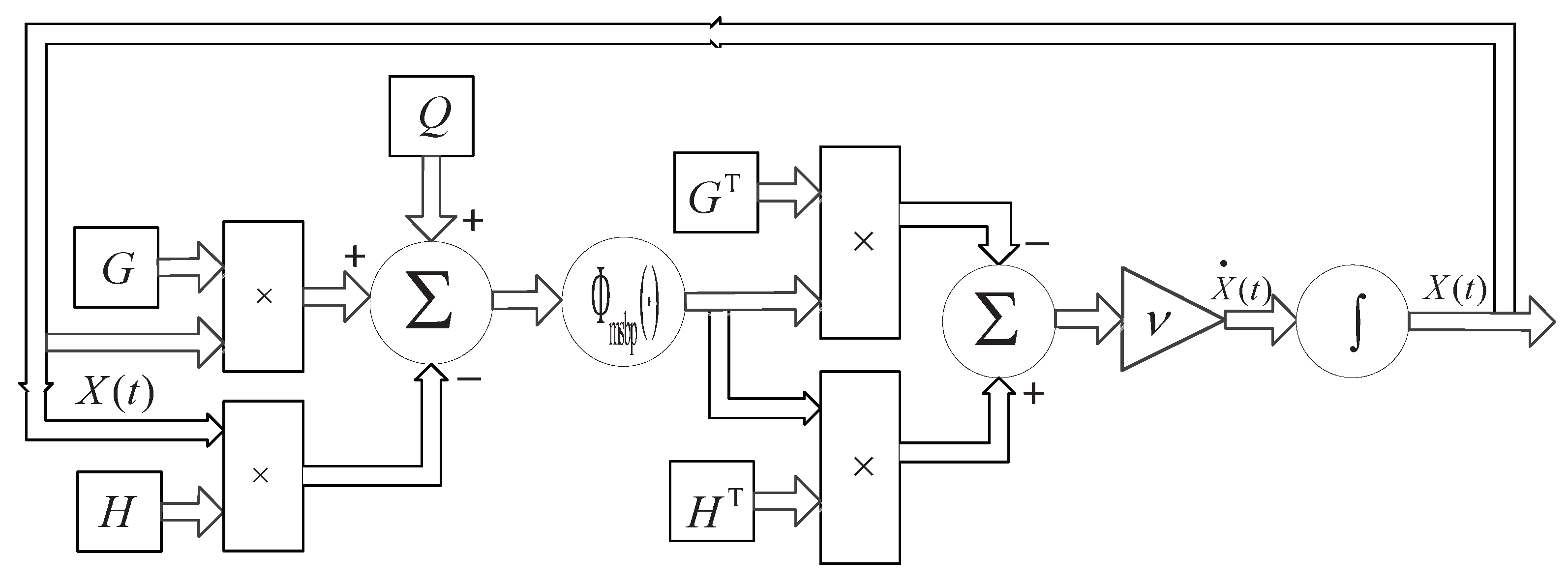
For a better understanding of the presented GNN model (9), we illustrate the block diagram realization of the GNN model (9) in Figure 1. In this figure, symbols ×, ∑, and ∫ are adopted to indicate matrix multiplication, the accumulator, and the integrator, respectively. $\mathbf{G}$, $\mathbf{H}$, and $\mathbf{Q}$ are given matrices and could be viewed as the input of the GNN model (9). $\mathbf{X}\left(t\right)$ is the neural state matrix and output of GNN model (9), while $\dot{\mathbf{X}}\left(t\right)$ is the time derivative of $\mathbf{X}\left(t\right)$. In addition, ${\mathsf{\Phi }}_{\mathrm{msbp}}(·)$ is the activation function array and defined element-wise. That is, ${\mathsf{\Phi }}_{\mathrm{msbp}}\left(\mathbf{U}\right)=\left[{\varphi }_{\mathrm{msbp}}\left(u_{ij}\right)\right]\in {\mathbb{R}}^{m\times n}$ for matrix $\mathbf{U}=\left[u_{ij}\right]\in {\mathbb{R}}^{m\times n}$. As time elapses, $\mathbf{X}\left(t\right)$ with any initial value, $\mathbf{X}\left(0\right)$ will converge to the theoretical solution of the Sylvester equation. (This point will be illustrated in the manner of mathematical derivation and simulation verification in the next sections.) Furthermore, to better illustrate the differences between the GNN model (9) and other GNN models (i.e., GNN models (5) and (6)) as well as the novelties and contributions of this work, the comparison of these three GNN models is summarized in

Table 1. Comparison of GNN models (5), (6), and (9) for solving Sylvester equation.

GNN Model	Activation Function	Convergence Property
(5)	$\varphi \left(u\right)=u$	exponential (infinite-time)
(6)	${\varphi }_{\mathrm{sbp}}\left(u\right)$ (7)	fixed-time
(9)	${\varphi }_{\mathrm{msbp}}\left(u\right)$ (8)	faster fixed-time

. When parameters are set as ${\eta }_1={\eta }_3=1,{\eta }_2=0,\sigma =1/\varrho$, GNN model (9) is simplified to GNN model (6). When ${\eta }_1={\eta }_3=0,{\eta }_2=1$, GNN model (9) is simplified to GNN model (5). It can thus be concluded that GNN model (9) is a more general model that incorporates GNN models (5) and (6) as special cases. In addition, as illustrated in Table 1, the presented GNN model (9) is superior to GNN models (5) and (6) in terms of convergence.

Remark 2.

Continuous-time GNN models (5), (6), and (9) are computational schemes. On one hand, a computational scheme can be generally treated as a neural network if it is realized by a hardware circuit (analog circuit and/or digital circuit) in an interconnecting way [41]. Considering potential hardware implementation, the above comparison of the three GNN models is significant and of practical relevance. On the other hand, such a computational scheme can be regarded as a numerical algorithm if it is realized by a serial computing computer program and executed on a digital computer [41]. For the development of effective numerical algorithms, discrete-time GNN models with convergence and high precision need to be obtained, which is one of the future research directions.

3. Theoretical Analysis

In this section, a theorem in terms of the convergence performance of the presented FTC-GNN model (9) is first provided and proven. Then, for comparative purposes, two propositions concerning the convergence properties of GNN models (5) and (6) are also offered.

Theorem 1.

Given matrices $\mathbf{G}\in {\mathbb{R}}^{m\times m}$, $\mathbf{H}\in {\mathbb{R}}^{n\times n}$, and $\mathbf{Q}\in {\mathbb{R}}^{m\times n}$ of Sylvester Equation (4), GNN model (9) can achieve global fixed-time convergence, i.e., the neural solution $\mathbf{X}\left(t\right)$ of GNN model (9) with any initial value $\mathbf{X}\left(0\right)$ globally reaches the theoretical solution ${\mathbf{X}}^{*}$ within a predetermined time

$$\begin{array}{c}\hfill T_{\max }=\frac{ln[1+\frac{{\eta }_2}{{\eta }_3}{\left(\frac{mn}{2\lambda }\right)}^{\frac{\sigma -1}{2}}]}{\nu {\eta }_2\lambda (\sigma -1)}+\frac{ln[1+\frac{{\eta }_2}{{\eta }_1}{\left(2\lambda \right)}^{\frac{1-\varrho }{2}}]}{\nu {\eta }_2\lambda (1-\varrho )},\end{array}$$

where $\lambda >0$ is the minimum eigenvalue of symmetric matrix ${\mathbf{W}}^{\mathrm{T}}\mathbf{W}$ with $\mathbf{W}:={\mathbf{I}}_n\otimes \mathbf{G}-{\mathbf{H}}^{\mathrm{T}}\otimes {\mathbf{I}}_m$ and ${\mathbf{I}}_n$ denoted the n-by-n identity matrix.

Proof of Theorem 1.

First, $\mathbf{y}\left(t\right):=\mathrm{vec}\left(\mathbf{X}\left(t\right)\right)\in {\mathbb{R}}^{mn},{\mathbf{y}}^{*}:=\mathrm{vec}\left({\mathbf{X}}^{*}\right)\in {\mathbb{R}}^{mn}$, and solution error $\overline{\mathbf{y}}\left(t\right):=\mathbf{y}\left(t\right)-{\mathbf{y}}^{*}$ are defined, where $\mathrm{vec}(·)$ and ${\mathbf{X}}^{*}$ separately denote the vectorization operator [36,40] and the unique exact solution of Sylvester Equation (4). Vectorizing the GNN model (9) by the Kronecker product denoted by symbol ⊗ yields

$$\begin{array}{cc}\hfill \dot{\overline{\mathbf{y}}}\left(t\right)& =\dot{\mathbf{y}}\left(t\right)\hfill \\ \hfill & =-\nu \left(({\mathbf{I}}_n\otimes {\mathbf{G}}^{\mathrm{T}})-(\mathbf{H}\otimes {\mathbf{I}}_m)\right)\mathrm{vec}\left({\mathsf{\Phi }}_{\mathbf{msbp}}(\mathbf{GX}\left(t\right)-\mathbf{X}\left(t\right)\mathbf{H}+\mathbf{Q})\right)\hfill \\ \hfill & =-\nu \left(({\mathbf{I}}_n\otimes {\mathbf{G}}^{\mathrm{T}})-(\mathbf{H}\otimes {\mathbf{I}}_m)\right){\mathsf{\Phi }}_{\mathbf{msbp}}^{\mathbf{v}}\left(\mathrm{vec}\left(\mathbf{GX}\right(t)-\mathbf{X}(t)\mathbf{H}+\mathbf{Q})\right)\hfill \\ \hfill & =-\nu \left(({\mathbf{I}}_n\otimes {\mathbf{G}}^{\mathrm{T}})-(\mathbf{H}\otimes {\mathbf{I}}_m)\right){\mathsf{\Phi }}_{\mathbf{msbp}}^{\mathbf{v}}\left(\left(({\mathbf{I}}_n\otimes \mathbf{G})-({\mathbf{H}}^{\mathrm{T}}\otimes {\mathbf{I}}_m)\right)(\mathbf{y}\left(t\right)-{\mathbf{y}}^{*})\right)\hfill \\ \hfill & =-\nu {\mathbf{W}}^{\mathrm{T}}{\mathsf{\Phi }}_{\mathbf{msbp}}^{\mathbf{v}}\left(\mathbf{W}\overline{\mathbf{y}}\left(t\right)\right).\hfill \end{array}$$

(10)

where $\mathbf{W}:={\mathbf{I}}_n\otimes \mathbf{G}-{\mathbf{H}}^{\mathrm{T}}\otimes {\mathbf{I}}_m$, with ${\mathbf{I}}_n$ denoted the n-by-n identity matrix, and ${\mathsf{\Phi }}_{\mathbf{msbp}}^{\mathbf{v}}(·)=\mathrm{vec}\left({\mathsf{\Phi }}_{\mathbf{msbp}}(·)\right)\in {\mathbb{R}}^{mn}$.

Now, $L\left(t\right)=\parallel \overline{\mathbf{y}}{\left(t\right)\parallel }_2^2/2\ge 0$ is selected as the Lyapunov function candidate [36]. It is easy to conclude that $L\left(t\right)$ is positive definite and $\mathbf{y}\left(t\right)\to \infty$, $L\left(t\right)\to \infty$. The calculation of the time derivative of $L\left(t\right)$ along the state trajectory of system (10) is given as follows:

$$\begin{array}{cc}\hfill \dot{L}\left(t\right)& ={\overline{\mathbf{y}}}^{\mathrm{T}}\left(t\right)\dot{\overline{\mathbf{y}}}\left(t\right)\hfill \\ \hfill & =-\nu {\overline{\mathbf{y}}}^{\mathrm{T}}\left(t\right){\mathbf{W}}^{\mathrm{T}}{\mathsf{\Phi }}_{\mathbf{msbp}}^{\mathbf{v}}\left(\mathbf{W}\overline{\mathbf{y}}\left(t\right)\right)\hfill \\ \hfill & =-\nu {\left(\mathbf{W}\overline{\mathbf{y}}\left(t\right)\right)}^{\mathrm{T}}{\mathsf{\Phi }}_{\mathbf{msbp}}^{\mathbf{v}}\left(\mathbf{W}\overline{\mathbf{y}}\left(t\right)\right)\hfill \\ \hfill & =-\nu \sum _{i=1}^{mn}{\left[\mathbf{W}\overline{\mathbf{y}}\left(t\right)\right]}_i·{\varphi }_{\mathrm{msbp}}\left({\left[\mathbf{W}\overline{\mathbf{y}}\left(t\right)\right]}_i\right)\hfill \\ \hfill & =-\nu \sum _{i=1}^{mn}|{\left[\mathbf{W}\overline{\mathbf{y}}\left(t\right)\right]}_i|·({\eta }_1|{\left[\mathbf{W}\overline{\mathbf{y}}\left(t\right)\right]}_i{|}^{\varrho }+{\eta }_2|{\left[\mathbf{W}\overline{\mathbf{y}}\left(t\right)\right]}_i|+{\eta }_3|{\left[\mathbf{W}\overline{\mathbf{y}}\left(t\right)\right]}_i{|}^{\sigma })\hfill \\ \hfill & =-\nu {\eta }_1\sum _{i=1}^{mn}{\left({\left[\mathbf{W}\overline{\mathbf{y}}\left(t\right)\right]}_i^2\right)}^{\frac{1+\varrho }{2}}-\nu {\eta }_2\sum _{i=1}^{mn}\left({\left[\mathbf{W}\overline{\mathbf{y}}\left(t\right)\right]}_i^2\right)-\nu {\eta }_3\sum _{i=1}^{mn}{\left({\left[\mathbf{W}\overline{\mathbf{y}}\left(t\right)\right]}_i^2\right)}^{\frac{1+\sigma }{2}}\hfill \\ \hfill & \le -\nu {\eta }_1{\left(\sum _{i=1}^{mn}{\left[\mathbf{W}\overline{\mathbf{y}}\left(t\right)\right]}_i^2\right)}^{\frac{1+\varrho }{2}}-\nu {\eta }_2\left({\overline{\mathbf{y}}}^{\mathrm{T}}\left(t\right){\mathbf{W}}^{\mathrm{T}}\mathbf{W}\overline{\mathbf{y}}\left(t\right)\right)\hfill \\ \hfill & -\nu {\eta }_3{\left(mn\right)}^{\frac{1-\sigma }{2}}{\left(\sum _{i=1}^{mn}{\left[\mathbf{W}\overline{\mathbf{y}}\left(t\right)\right]}_i^2\right)}^{\frac{1+\sigma }{2}}\hfill \\ \hfill & =-\nu {\eta }_1{\left({\overline{\mathbf{y}}}^{\mathrm{T}}\left(t\right){\mathbf{W}}^{\mathrm{T}}\mathbf{W}\overline{\mathbf{y}}\left(t\right)\right)}^{\frac{1+\varrho }{2}}-\nu {\eta }_2\left({\overline{\mathbf{y}}}^{\mathrm{T}}\left(t\right){\mathbf{W}}^{\mathrm{T}}\mathbf{W}\overline{\mathbf{y}}\left(t\right)\right)\hfill \\ \hfill & -\nu {\eta }_3{\left(mn\right)}^{\frac{1-\sigma }{2}}{\left({\overline{\mathbf{y}}}^{\mathrm{T}}\left(t\right){\mathbf{W}}^{\mathrm{T}}\mathbf{W}\overline{\mathbf{y}}\left(t\right)\right)}^{\frac{1+\sigma }{2}}\hfill \\ \hfill & \le -\nu {\eta }_1{2}^{\frac{1+\varrho }{2}}{\lambda }^{\frac{1+\varrho }{2}}{L}^{\frac{1+\varrho }{2}}\left(t\right)-2\nu {\eta }_2\lambda L\left(t\right)-\nu {\eta }_3{\left(mn\right)}^{\frac{1-\sigma }{2}}{2}^{\frac{1+\sigma }{2}}{\lambda }^{\frac{1+\sigma }{2}}{L}^{\frac{1+\sigma }{2}}\left(t\right)\hfill \\ \hfill & =-p{L}^{\frac{1+\varrho }{2}}\left(t\right)-qL\left(t\right)-r{L}^{\frac{1+\sigma }{2}}\left(t\right)\le 0,\hfill \end{array}$$

(11)

where $\lambda >0$ represents the minimum eigenvalue of symmetric matrix ${\mathbf{W}}^{\mathrm{T}}\mathbf{W}$. In addition, $p=\nu {\eta }_1{2}^{\frac{1+\varrho }{2}}{\lambda }^{\frac{1+\varrho }{2}}$, $q=2\nu {\eta }_2\lambda$, and $r=\nu {\eta }_3{\left(mn\right)}^{\frac{1-\sigma }{2}}{2}^{\frac{1+\sigma }{2}}{\lambda }^{\frac{1+\sigma }{2}}$. It is noted that Lemma 1 has been adopted where the symbol ≤ first appears. The above analysis implies that Lemma 3 applies, and a conclusion is thus drawn that the unique equilibrium point $\overline{\mathbf{y}}\left(t\right)=\mathbf{0}$ is globally fixed-time stable. Furthermore, we have

$$\begin{array}{cc}\hfill T_{\max }& =\frac{ln[1+\frac{q}{r}]}{q\left(\right(1+\sigma )/2-1)}+\frac{ln[1+\frac{q}{p}]}{q(1-(1+\varrho )/2)}\hfill \\ \hfill & =\frac{ln[1+\frac{{\eta }_2}{{\eta }_3}{\left(\frac{mn}{2\lambda }\right)}^{\frac{\sigma -1}{2}}]}{\nu {\eta }_2\lambda (\sigma -1)}+\frac{ln[1+\frac{{\eta }_2}{{\eta }_1}{\left(2\lambda \right)}^{\frac{1-\varrho }{2}}]}{\nu {\eta }_2\lambda (1-\varrho )}.\hfill \end{array}$$

(12)

In light of $\overline{\mathbf{y}}\left(t\right)=\mathbf{y}\left(t\right)-{\mathbf{y}}^{*}=\mathrm{vec}\left(\mathbf{X}\left(t\right)\right)-\mathrm{vec}\left({\mathbf{X}}^{*}\right)$, the conclusion is obtained that $\mathbf{X}\left(t\right)$ is globally fixed-time convergent to the theoretical solution ${\mathbf{X}}^{*}$. The proof is thus completed. □

Proposition 1

([30,40]). Given matrices $\mathbf{G}\in {\mathbb{R}}^{m\times m}$, $\mathbf{H}\in {\mathbb{R}}^{n\times n}$, and $\mathbf{Q}\in {\mathbb{R}}^{m\times n}$ of Sylvester Equation (4), linear GNN model (5) can attain global exponential convergence, i.e., the neural solution $\mathbf{X}\left(t\right)$ of linear GNN model (5) with any initial value $\mathbf{X}\left(0\right)$ is globally exponentially convergent to the theoretical solution ${\mathbf{X}}^{*}$, with the exponential convergence rate being $\nu \lambda$, where $\lambda >0$ is the minimum eigenvalue of matrix ${\mathbf{W}}^{\mathrm{T}}\mathbf{W}$ with $\mathbf{W}:={\mathbf{I}}_n\otimes \mathbf{G}-{\mathbf{H}}^{\mathrm{T}}\otimes {\mathbf{I}}_m$ and ${\mathbf{I}}_n$ denoting the n-by-n identity matrix.

Proposition 2.

Given matrices $\mathbf{G}\in {\mathbb{R}}^{m\times m}$, $\mathbf{H}\in {\mathbb{R}}^{n\times n}$, and $\mathbf{Q}\in {\mathbb{R}}^{m\times n}$ of Sylvester Equation (4), GNN model (6) can achieve global fixed-time convergence, i.e., the neural solution $\mathbf{X}\left(t\right)$ of GNN model (6) with any initial value $\mathbf{X}\left(0\right)$ globally reaches the theoretical solution ${\mathbf{X}}^{*}$ within a predetermined time

$$\begin{array}{c}\hfill T_{\max }=\frac{2}{{\left(2\lambda \right)}^{\frac{1+\varrho }{2}}\nu (1-\varrho )}+\frac{2\varrho }{{\left(mn\right)}^{\frac{\varrho -1}{2\varrho }}{\left(2\lambda \right)}^{\frac{1+\varrho }{2\varrho }}\nu (1-\varrho )},\end{array}$$

where $\lambda >0$ is the minimum eigenvalue of symmetric matrix ${\mathbf{W}}^{\mathrm{T}}\mathbf{W}$ with $\mathbf{W}:={\mathbf{I}}_n\otimes \mathbf{G}-{\mathbf{H}}^{\mathrm{T}}\otimes {\mathbf{I}}_m$ and ${\mathbf{I}}_n$ denoting the n-by-n identity matrix.

Proof of Proposition 2.

See Appendix A for details. □

Remark 3.

In light of the above theoretical results, we know that the sbp function activated GNN model (6) with declared finite-time convergence in the previous work [33] is, in fact, of fixed-time convergence. Furthermore, if ${\eta }_1={\eta }_3=1$ and $\sigma =1/\varrho$ are set for the msbp function, based on Remark 1, it is easy to see that GNN model (9) has faster fixed-time convergence as compared to GNN model (6), which theoretically ensures its superior convergence performance.

4. Numerical Simulations

In this section, two illustrative examples are simulated to demonstrate the theoretical results presented in the above section.

4.1. Example 1

The Sylvester Equation (4) with the following 2-by-2 coefficient matrices and theoretical solution ${\mathbf{X}}^{*}$ is investigated as an example:

$$\mathbf{G}=\left[\begin{array}{cc}2& 1\\ -1& 1\end{array}\right],\mathbf{H}=\left[\begin{array}{cc}2& 3\\ 4& 5\end{array}\right],\mathbf{Q}=\left[\begin{array}{cc}10& 2\\ 1& 0\end{array}\right],{\mathbf{X}}^{*}=\left[\begin{array}{cc}-1& 2\\ -2& 1\end{array}\right].$$

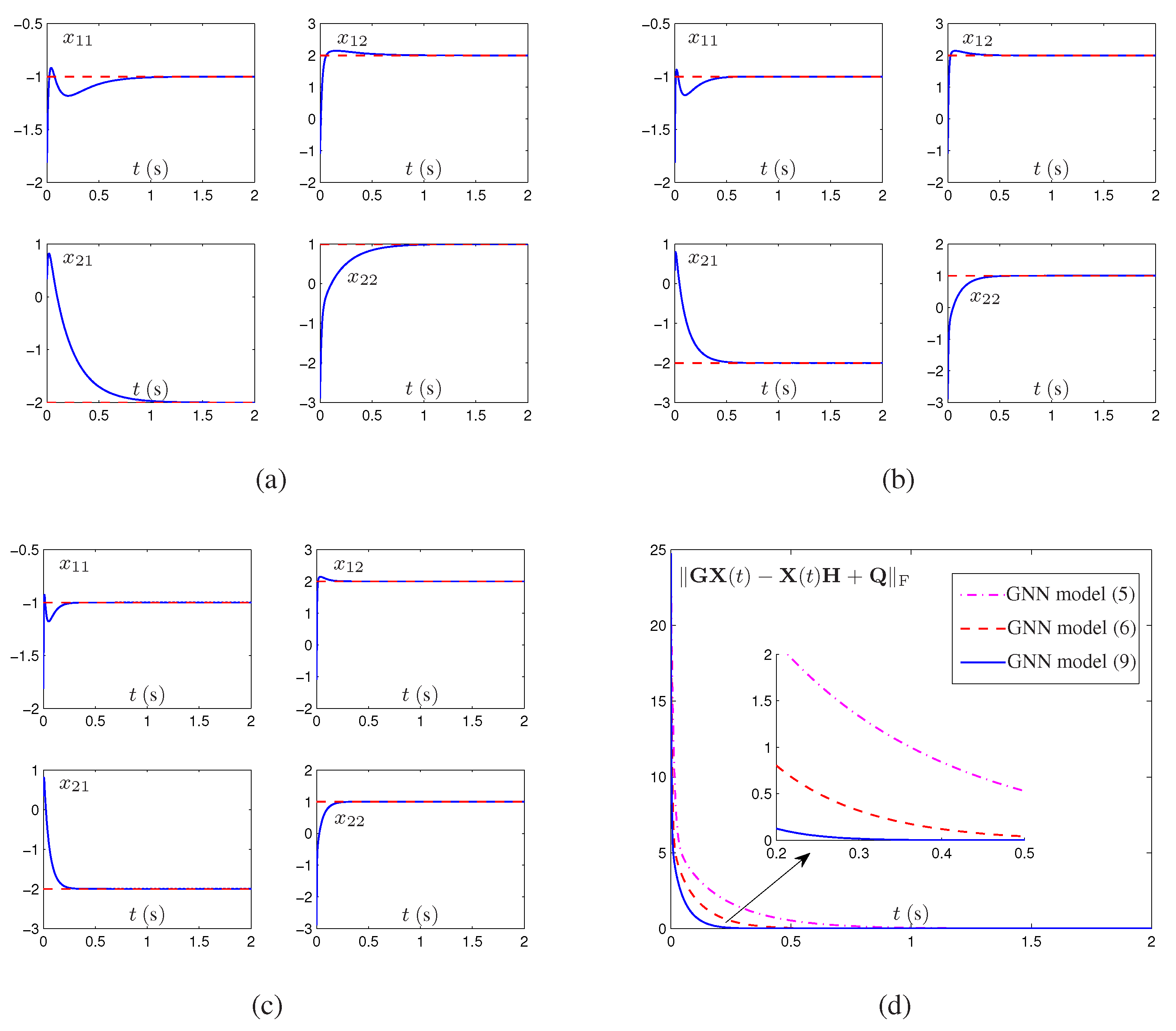
It is easy to see that the minimum eigenvalue of matrix ${\mathbf{W}}^{\mathrm{T}}\mathbf{W}$ is $\lambda =2.3020$. For a fair comparison, the design parameters of GNN models (5), (6), and (9) are set as $\nu =2$, ${\eta }_1={\eta }_3=1,{\eta }_2=2,\varrho =0.8,\sigma =1/\varrho =1.25$. Starting with an initial state $\mathbf{X}\left(0\right)$ generated randomly from ${[-5,5]}^{2\times 2}$, GNN models (5), (6), and the presented GNN model (9) are successively put to use to solve the Sylvester equation, with the simulation duration being 2 s. The convergence behaviors of neural state $\mathbf{X}\left(t\right)$ and residual error ${\parallel \mathbf{G}\mathbf{X}\left(t\right)-\mathbf{X}\left(t\right)\mathbf{H}+\mathbf{Q}\parallel }_{\mathrm{F}}$ are shown in Figure 2, which well substantiates the superior convergence of the presented GNN model (9).

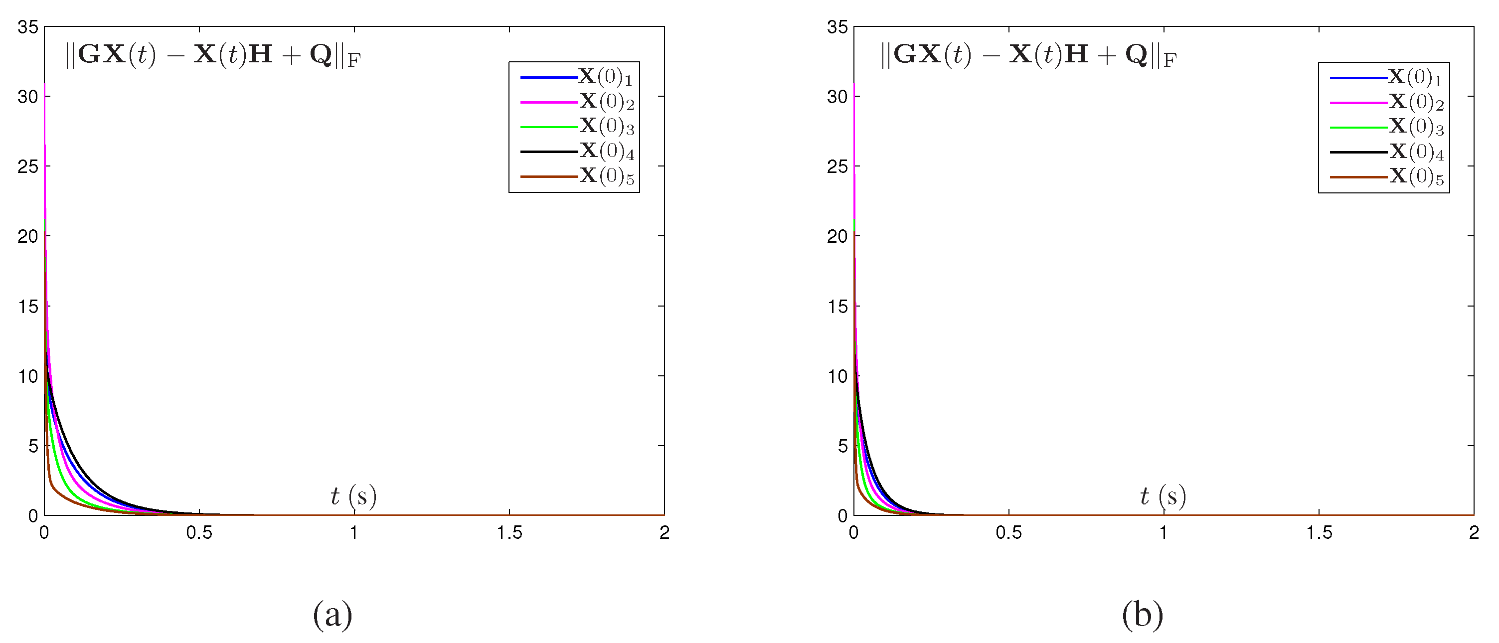
Then, to demonstrate the fixed-time convergence property of GNN models (6) and (9), five values in the range of ${[-5,5]}^{2\times 2}$ are randomly created and used for the initial states of $\mathbf{X}\left(t\right)$ (i.e., $\mathbf{X}{\left(0\right)}_1\sim \mathbf{X}{\left(0\right)}_5$). Model parameters involved remain the same. According to the theoretical analysis results, the upper bounds of the convergence time of GNN models (6) and (9) are, respectively, $T_{\max }\approx 2.12$ s and $T_{\max }\approx 1.13$ s. Figure 3 illustrates the change process of residual error ${\parallel \mathbf{G}\mathbf{X}\left(t\right)-\mathbf{X}\left(t\right)\mathbf{H}+\mathbf{Q}\parallel }_{\mathrm{F}}$. As expected, residual errors ${\parallel \mathbf{G}\mathbf{X}\left(t\right)-\mathbf{X}\left(t\right)\mathbf{H}+\mathbf{Q}\parallel }_{\mathrm{F}}$ are convergent to 0 within $T_{\max }$ for the both GNN models, which verifies the correctness of Theorem 1 and Proposition 2. Furthermore, comparing Figure 3a,b, it can be observed again that the GNN model (9) outperforms the GNN model (6) in terms of convergence performance.

4.2. Example 2

In this subsection, a higher-dimensional example with the following coefficient matrices and the theoretical solution is investigated to further demonstrate the superiority and fixed-time convergence property of the presented GNN model (9):

$$\mathbf{G}=\left[\begin{array}{cccc}3.8881& 2.6582& 0.4725& 1.5207\\ 0.3931& 1.5262& 2.8427& 2.6915\\ 2.7392& 1.6217& 3.3560& 3.2598\\ 0.6112& 1.2168& 1.6013& 0.8726\end{array}\right],\mathbf{H}=\left[\begin{array}{cccc}0.7805& 5.6584& 2.9058& 1.0066\\ 5.5417& 3.1858& 3.7721& 1.2818\\ 3.5263& 3.0900& 0.0728& 4.6441\\ 2.2643& 0.3490& 5.5018& 5.3392\end{array}\right],$$

$$\mathbf{Q}=\left[\begin{array}{cccc}1.8506& 4.3380& 5.4336& 3.0296\\ 3.0259& 5.2791& 5.3998& 3.1585\\ 3.6453& 3.0072& 2.9610& 1.6716\\ 5.7793& 0.8481& 3.6165& 2.7530\end{array}\right],{\mathbf{X}}^{*}=\left[\begin{array}{cccc}0.8785& 0.4942& 0.7850& 1.2275\\ 1.3911& 0.4000& 0.5590& 0.9476\\ 0.9526& 0.7202& 1.0077& 1.0018\\ -0.2909& 1.1417& 0.5124& 0.6068\end{array}\right].$$

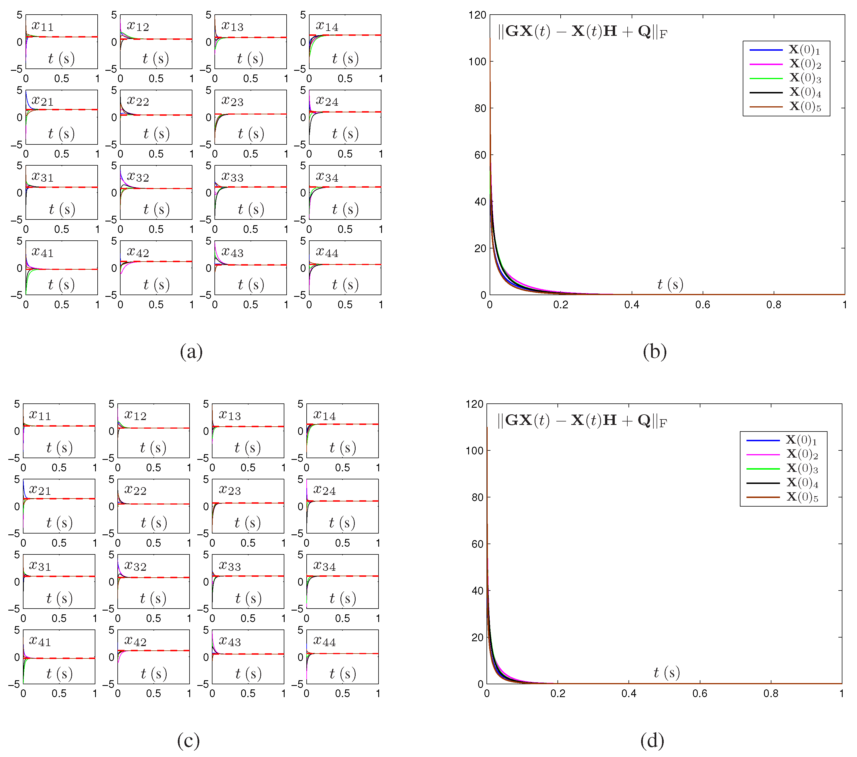
The minimum eigenvalue of matrix ${\mathbf{W}}^{\mathrm{T}}\mathbf{W}$ is obtained as $\lambda =6.3$. Parameter $\nu =1$, simulation duration is set as 1s, and other parameters remain the same as in Example 1. Then, starting from five different initial values randomly generated from ${[-5,5]}^{4\times 4}$, the GNN model (6) and the presented GNN model (9) are put to use for solving the above Sylvester equation. Transient behaviors of neural solution $\mathbf{X}\left(t\right)$ and residual error ${\parallel \mathbf{G}\mathbf{X}\left(t\right)-\mathbf{X}\left(t\right)\mathbf{H}+\mathbf{Q}\parallel }_{\mathrm{F}}$ synthesized by the two GNN models are visualized in Figure 4, which well illustrates the global convergence of the two GNN models. The superiority of the presented GNN model (9) over the GNN model (6) can be obviously observed from Figure 4b,d. In addition, for the presented GNN model (9), the residual errors ${\parallel \mathbf{G}\mathbf{X}\left(t\right)-\mathbf{X}\left(t\right)\mathbf{H}+\mathbf{Q}\parallel }_{\mathrm{F}}$ starting from five different initial neural states (i.e., $\mathbf{X}{\left(0\right)}_1\sim \mathbf{X}{\left(0\right)}_5$) are all able to arrive at 0 within $T_{\max }\approx 0.86$ s, which is shown in Figure 4d. The fixed-time convergence of the presented GNN model (9) is thus well demonstrated again.

In brief, the simulation results of the above two illustrative examples are in line with the theoretical analysis presented in Theorem 1 and Proposition 2.

5. Conclusions

Along the research direction of GNN, the GNN model (9) with fixed-time convergence is developed and analyzed to solve the Sylvester equation in this work. Such a model is under the action of the msbp function (8) and has the fastest convergence rate as compared to the linear GNN model (5) and the sbp function activated GNN model (6). Theorem 1 gives detailed mathematical analysis to demonstrate that the upper bound of the convergence time of the presented GNN model (9) is referable to the model parameters rather than the initial value of the neural state. Furthermore, this work also provides mathematical analysis to show the fixed-time convergence property of the GNN model (6). The fact that the GNN model (9) has faster fixed-time convergence as compared to the GNN model (6) is theoretically ensured by these mathematical analyses. Finally, the comparative simulation results given through two numerical examples substantiate the theoretical analysis, as well as the advantages of the presented GNN model over the existing GNN models (i.e., GNN models (5) and (6)) in terms of convergence performance. The development of more GNN models for handling other problems and the application of the presented GNN model (9) and/or extended models to the kinematic control of robot manipulators will be our research directions in the future. Another research direction would be the development of discrete-time GNN models with convergence and high precision.

References

- Wei, Q.; Dobigeon, N.; Tourneret, J.-Y.; Bioucas-Dias, J.; Godsill, S. R-FUSE: Robust fast fusion of multiband images based on solving a Sylvester equation. IEEE Signal Process. Lett. 2016, 23, 1632–1636. [Google Scholar] [CrossRef]
- Peralta, D.; Saeys, Y. Robust unsupervised dimensionality reduction based on feature clustering for single-cell imaging data. Appl. Soft Comput. 2020, 93, 106421. [Google Scholar] [CrossRef]
- Darouach, M. Solution to Sylvester equation associated to linear descriptor systems. Syst. Control Lett. 2016, 55, 835–838. [Google Scholar] [CrossRef]
- Chen, G.; Song, Y.; Wang, F.; Zhang, C. Semi-supervised multi-label learning by solving a Sylvester equation. In Proceedings of the 2008 SIAM International Conference on Data Mining (SDM), Atlanta, GA, USA, 24–26 April 2008; pp. 410–419. [Google Scholar]
- Natarajan, V. Compensating PDE actuator and sensor dynamics using Sylvester equation. Automatica 2021, 123, 109362. [Google Scholar] [CrossRef]
- Kittisopaporn, A.; Chansangiam, P.; Lewkeeratiyutkul, W. Convergence analysis of gradient-based iterative algorithms for a class of rectangular Sylvester matrix equations based on Banach contraction principle. Adv. Differ. Equ. 2021, 2021, 17. [Google Scholar] [CrossRef]
- Zhang, J.; Luo, X. Gradient-based optimization algorithm for solving Sylvester matrix equation. Mathematics 2022, 10, 1040. [Google Scholar] [CrossRef]
- Bartels, R.H.; Stewart, G.W. Solution of the matrix equation AX + XB = C. Commun. ACM 1972, 15, 820–826. [Google Scholar] [CrossRef]
- Kleinman, D.; Rao, P.K. Extensions to the Bartels–Stewart algorithm for linear matrix equations. IEEE Trans. Autom. Control 1978, 23, 85–87. [Google Scholar] [CrossRef]
- Stykel, T. Numerical solution and perturbation theory for generalized Lyapunov equations. Linear Algebra Appl. 2002, 349, 155–185. [Google Scholar] [CrossRef]
- Mathews, J.H.; Fink, K.D. Numerical Methods Using MATLAB; Pretice Hall: Hoboken, NJ, USA, 2004. [Google Scholar]
- Li, S.; Li, Y. Nonlinearly activated neural network for solving time-varying complex Sylvester equation. IEEE Trans. Cybern. 2014, 44, 1397–1407. [Google Scholar] [CrossRef]
- Atencia, M.; Boumeridja, H.; Joya, G.; García-Lagos, F.; Sandoval, F. FPGA implementation of a systems identification module based upon Hopfield networks. Neurocomputing 2007, 70, 2828–2835. [Google Scholar] [CrossRef]
- Ortega-Zamorano, F.; Jerez, J.M.; Franco, L. FPGA implementation of the C-Mantec neural network constructive algorithm. IEEE Trans. Ind. Inform. 2014, 10, 1154–1161. [Google Scholar] [CrossRef]
- Che, H.; Wang, J. A two-timescale duplex neurodynamic approach to biconvex optimization. IEEE Trans. Neural Netw. Learn. Syst. 2019, 30, 2503–2514. [Google Scholar] [CrossRef]
- Zhang, Y.; Jiang, D.; Wang, J. A recurrent neural network for solving Sylvester equation with time-varying coefficients. IEEE Trans. Neural Netw. 2002, 13, 1053–1063. [Google Scholar] [CrossRef] [PubMed]
- Li, S.; Chen, S.; Liu, B. Accelerating a recurrent neural network to finite-time convergence for solving time-varying Sylvester equation by using a sign-bi-power activation function. Neural Process Lett. 2013, 37, 189–205. [Google Scholar] [CrossRef]
- Xiao, L.; Zhang, Y.; Dai, J.; Li, J.; Li, W. New noise-tolerant ZNN models with predefined-time convergence for time-variant Sylvester equation solving. IEEE Trans. Syst. Man Cybern. Syst. 2021, 51, 3629–3640. [Google Scholar] [CrossRef]
- Lei, Y.; Dai, Z.; Liao, B.; Xia, G.; He, Y. Double features zeroing neural network model for solving the pseudoninverse of a complex-valued time-varying matrix. Mathematics 2022, 10, 2122. [Google Scholar] [CrossRef]
- Xiao, L.; He, Y. A Noise-suppression ZNN model with new variable parameter for dynamic Sylvester equation. IEEE Trans. Ind. Inform. 2021, 17, 7513–7522. [Google Scholar] [CrossRef]
- Xiao, L.; Tao, J.; Li, W. An arctan-type varying-parameter ZNN for solving time-varying complex Sylvester equations in finite time. IEEE Trans. Ind. Inform. 2022, 18, 3651–3660. [Google Scholar] [CrossRef]
- Tan, Z.; Li, W.; Xiao, L.; Hu, Y. New varying-parameter ZNN models with finite-time convergence and noise suppression for time-varying matrix Moore-Penrose inversion. IEEE Trans. Neural Netw. Learn. Syst. 2020, 31, 2980–2992. [Google Scholar] [CrossRef]
- Gerontitis, D.; Behera, R.; Tzekis, P.; Stanimirović, P. A family of varying-parameter finite-time zeroing neural networks for solving time-varying Sylvester equation and its application. J. Comput. Appl. Math. 2022, 403, 113826. [Google Scholar] [CrossRef]
- Zhang, Z.; Zheng, L. A complex varying-parameter convergent-differential neural-network for solving online time-varying complex Sylvester equation. IEEE Trans. Cybern. 2019, 49, 3627–3639. [Google Scholar] [CrossRef] [PubMed]
- He, Y.; Liao, B.; Xiao, L.; Han, L.; Xiao, X. Double accelerated convergence ZNN with noise-suppression for handling dynamic matrix inversion. Mathematics 2022, 10, 50. [Google Scholar] [CrossRef]
- Shi, Y.; Jin, L.; Li, S.; Qiang, J. Proposing, developing and verification of a novel discrete-time zeroing neural network for solving future augmented Sylvester matrix equation. J. Frankl. Inst. 2020, 357, 3636–3655. [Google Scholar] [CrossRef]
- Xiao, L.; Huang, W.; Jia, L.; Li, X. Two discrete ZNN models for solving time-varying augmented complex Sylvester equation. Neurocomputing 2022, 487, 280–288. [Google Scholar] [CrossRef]
- Qi, Y.; Jin, L.; Li, H.; Li, Y.; Liu, M. Discrete computational neural dynamics models for solving time-dependent Sylvester equation with applications to robotics and MIMO systems. IEEE Trans. Ind. Inform. 2020, 16, 6231–6241. [Google Scholar] [CrossRef]
- Shi, Y.; Jin, L.; Li, S.; Li, J.; Qiang, J.; Gerontitis, D.K. Novel discrete-time recurrent neural networks handling discrete-form time-variant multi-augmented Sylvester matrix problems and manipulator application. IEEE Trans. Neural Netw. Learn Syst. 2022, 33, 587–599. [Google Scholar] [CrossRef]
- Zhang, Y.; Yang, Y.; Chen, K.; Cai, B. MATLAB simulation of gradient-based neural network for Sylvester equation solving. J. Syst. Simul. 2009, 21, 4028–4031, 4037. (In Chinese) [Google Scholar]
- Liu, B.; Fu, D.; Qi, Y.; Huang, H.; Jin, L. Noise-tolerant gradient-oriented neurodynamic model for solving the Sylvester equation. Appl. Soft Comput. 2021, 109, 107514. [Google Scholar] [CrossRef]
- Liao, S.; Liu, J.; Xiao, X.; Fu, D.; Wang, G.; Jin, L. Modified gradient neural networks for solving the time-varying Sylvester equation with adaptive coefficients and elimination of matrix inversion. Neurocomputing 2020, 379, 1–11. [Google Scholar] [CrossRef]
- Xiao, L.; Liao, B.; Luo, J.; Ding, L. A convergence-enhanced gradient neural network for solving Sylvester equation. In Proceedings of the 36th Chinese Control Conference, Dalian, China, 26–28 July 2017; pp. 3910–3913. [Google Scholar]
- Lv, L.; Chen, J.; Zhang, L.; Zhang, F. Gradient-based neural networks for solving periodic Sylvester matrix equations. J. Frankl. Inst. 2022; in press. [Google Scholar] [CrossRef]
- Shen, Y.; Miao, P.; Huang, Y.; Shen, Y. Finite-time stability and its application for solving time-varying Sylvester equation by recurrent neural network. Neural Process. Lett. 2015, 42, 763–784. [Google Scholar] [CrossRef]
- Tan, Z.; Hu, Y.; Chen, K. On the investigation of activation functions in gradient neural network for online solving linear matrix equation. Neurocomputing 2020, 413, 185–192. [Google Scholar] [CrossRef]
- Polyakov, A. Nonlinear feedback design for fixed-time stabilization of linear control systems. IEEE Trans. Autom. Control 2012, 57, 2106–2110. [Google Scholar] [CrossRef]
- Chen, C.; Li, L.; Peng, H.; Yang, Y. Fixed-time synchronization of inertial memristor-based neural networks with discrete delay. Neural Netw. 2019, 109, 81–89. [Google Scholar] [CrossRef]
- Hardy, G.; Littlewood, J.; Polya, G. Inequalities; Cambridge University Press: Cambridge, UK, 1952. [Google Scholar]
- Chen, K. Improved neural dynamics for online Sylvester equations solving. Inf. Process. Lett. 2016, 116, 455–459. [Google Scholar] [CrossRef]
- Qiu, B.; Zhang, Y.; Yang, Z. New discrete-time ZNN models for least-squares solution of dynamic linear equation system with time-varying rank-deficient coefficient. IEEE Trans. Neural Netw. Learn. Syst. 2018, 29, 5767–5776. [Google Scholar] [CrossRef] [PubMed]
Figure 1.
Block diagram of GNN model (9) for solving Sylvester equation.
Figure 2.
Convergence behaviors of neural state denoted by blue solid curves and residual error . (a) Neural state of GNN model (5). (b) Neural state of GNN model (6). (c) Neural state of GNN model (9). (d) Residual error of three GNN models.
Figure 3.
Convergence behaviors of residual error of GNN models (6) and (9) starting from 5 randomly created initial values (i.e., ) for Sylvester equation. (a) By GNN model (6). (b) By GNN model (9).
Figure 4.
Convergence behaviors of neural state and residual error of GNN models (6) and (9) starting from 5 randomly created initial values for Sylvester equation in example 2, where red dashed lines denote the exact solution. (a) Neural state of GNN model (6). (b) Residual error of GNN model (6). (c) Neural state of GNN model (9). (d) Residual error of GNN model (9).
Publisher’s Note: MDPI stays neutral with regard to jurisdictional claims in published maps and institutional affiliations. |
© 2022 by the author. Licensee MDPI, Basel, Switzerland. This article is an open access article distributed under the terms and conditions of the Creative Commons Attribution (CC BY) license (https://creativecommons.org/licenses/by/4.0/).
Share and Cite
MDPI and ACS Style
Tan, Z. Fixed-Time Convergent Gradient Neural Network for Solving Online Sylvester Equation. Mathematics 2022, 10, 3090. https://doi.org/10.3390/math10173090
AMA Style
Tan Z. Fixed-Time Convergent Gradient Neural Network for Solving Online Sylvester Equation. Mathematics. 2022; 10(17):3090. https://doi.org/10.3390/math10173090
Chicago/Turabian StyleTan, Zhiguo. 2022. "Fixed-Time Convergent Gradient Neural Network for Solving Online Sylvester Equation" Mathematics 10, no. 17: 3090. https://doi.org/10.3390/math10173090
Note that from the first issue of 2016, this journal uses article numbers instead of page numbers. See further details here.