Inferences of the Multicomponent Stress–Strength Reliability for Burr XII Distributions

Abstract

Multicomponent stress–strength reliability (MSR) is explored for the system with Burr XII distributed components under Type-II censoring. When the distributions of strength and stress variables have Burr XII distributions with common or unequal inner shape parameters, the existence and uniqueness of the maximum likelihood estimators are investigated and established. The associated approximate confidence intervals are obtained by using the asymptotic normal distribution theory along with the delta method and parametric bootstrap procedure, respectively. Moreover, alternative generalized pivotal quantities-based point and confidence interval estimators are developed. Additionally, a likelihood ratio test is presented to diagnose the equivalence of both inner shape parameters or not. Conclusively, Monte Carlo simulations and real data analysis are conducted for illustration.

1. Introduction

The stress–strength model, under which a system or unit survives if its strength is greater than the stress imposed, plays a considerable role in lifetime studies, engineering applications, supply and demand applications, and others. The associated stress–strength reliability (SSR), R, is defined to be $R=P(Y<X)$, where X represents the strength of the system or unit and Y is the associated stress applied on it. Generally, the strength X is defined as the quality characteristics of the main subject and the stress is defined as the quality characteristics Y of the opposite subject in the model. To address the aforementioned stress–strength model, three examples are given for illustration. The first example is about mechanical engineering applications. The strength of the long horizontal part for a crane, denoted by X, is required to exceed the stress of loading weight of the lifting object for operation. We denote the stress of loading weight by Y. The SSR of $R=P(Y<X)$ can be an important measure for assessing the quality of crane. The second example is about civil engineering applications. The allowable bearing capacity of a suspension bridge is an important quality measure. The strength of a pairs of cables for the suspension bridge, denoted by X, should exceed the total amount of car weight passing through. We denote the stress of the total amount of car weight passing through by Y. In this application, a high SSR of $R=P(Y<X)$ is required for the design of the suspension bridge. The third example is about logistics applications. To maintain the quality of a logistics system, the supply capacity can be the strength, denoted by X, and the demand can be the stress, denoted by Y. A high SSR of $R=P(Y<X)$ indicates that the logistics system is reliable. Over the past few years, the stress–strength model has been extensively used in a variety of fields that include economics, hydrology, reliability engineering, seismology and survival analysis, and the inference of SSR had been discussed in numerous works; for example, by Eryilmaz [1], Kundu and Raqad [2], Krishnamoorthy and Lin [3], Mokhlis et al. [4], and Wang et al. [5]. Conventional studies for the SSR inference focus on the system of a sole main component, i.e., a unit. However, many practical systems, which include a series system, parallel system, or a combination of these two systems, are composed of multiple components to achieve their functions. Therefore, the SSR investigation has been extended to a multicomponent system. Generally, aforementioned multicomponent systems consist of k main components that have independent and identically distributed (i.i.d.) strengths subject to an opposite commonly distributed stress, and the system survives if at least $s(1\le s\le k)$ main components simultaneously function. In the literature, this system is usually referred to as the s-out-of-k G system.

In reality, there are many examples of a multicomponent system. For a communication system with three transmitters, the average message load may be such that at least two transmitters must be operational at all times; otherwise, critical messages may be lost. Thus, the transmission subsystem functions can be a 2-out-of-3 G system. Another example in the aircraft industry is that the Airbus A-380 has four engines and the airplane can fly if and only if at least two of its four engines are functioning, and this case is referred to as a 2-out-of-4 G system.

Let $X_1,X_2,\dots ,X_k$ denote the strength variables of k components in an s-out-of-k G system and follow a common cumulative distribution function (CDF), $F(·)$. Each component is subject to a stress, denoted by Y, which follows the CDF $G(·)$. Bhattacharyya and Johnson [6] provided the multicomponent stress–strength reliability (MSR), $R_{s,k}$, as follows:

$$\begin{array}{cc}\hfill R_{s,k}& =P\left(\mathrm{at}\mathrm{least}s\mathrm{of}\mathrm{the}(X_1,X_2,\dots ,X_k)\mathrm{exceed}Y\right)\hfill \\ \hfill & =\sum _{i=s}^k\left(\begin{array}{c}k\\ i\end{array}\right){\int }_{-\infty }^{\infty }{[1-F\left(t\right)]}^i{\left[F\left(t\right)\right]}^{k-i}dG\left(t\right).\hfill \end{array}$$

(1)

The s-out-of-k G system has attracted extensive attention and $R_{s,k}$ inference has been broadly investigated by numerous studies. These include multicomponent strength–stress models for Kumaraswamy distribution by Dey et al. [7], based on Chen distribution by Kayal [8], based on general class of inverse exponentiated distribution and proportional reversed hazard rate distribution by Kizilaslan [9,10], based on bivariate Kumaraswamy distribution by Kizilaslan and Nadar [11], based on Marshall-Olkin bivariate Weibull distribution by Nadar and Kizilaslan [12], based on Rayleigh stress–strength model by Rao [13], based on Burr XII distribution by Rao et al. [14], based on progressively Type-II censored samples from generalized Pareto distribution by Sauer et al. [15], and based on Rayleigh stress–strength model by Wang et al. [16].

The Burr XII distribution has gained much attention regarding the applications of modeling in reliability studies in recent decades. Let T be the Burr XII distributed random variable. Then, the CDF and probability density function (PDF) of T are respectively given as

$$\begin{array}{c}\hfill F(t;\lambda ,\alpha )=1-{(1+t^{\lambda })}^{-\alpha }\mathrm{and}f(t;\lambda ,\alpha )=\alpha \lambda t^{\lambda -1}{(1+t^{\lambda })}^{-(\alpha +1)},t>0,\end{array}$$

(2)

where $\lambda >0$ is the inner shape parameter and $\alpha >0$ is the outer shape parameter. For easy reference, the Burr XII distribution with parameters $\lambda >0$ and $\alpha >0$ will be denoted by BurrXII$(\lambda ,\alpha )$, hereafter. The BurrXII$(\lambda ,\alpha )$ was initially introduced by Burr [17]. Due to two shape parameters, the BurrXII$(\lambda ,\alpha )$ is a very important and flexible probability model for any positive random variable. Tadikamalla [18] provided the link of BurrXII$(\lambda ,\alpha )$ to some widely used lifetime distributions such as Weibull, chi-square, Rice, and extreme value models. Since then, many authors have investigated the inference methods with different applications of the Bur XII model. Kumar [19] studied the mathematical properties for the moment-generating function, conditional moments, mean residual time and mean past time, the mean deviation about mean and median, stochastic ordering, and SSR estimates for the Burr XII distribution. Lio and Tsai [20] investigated the SSR estimates using progressively first-failure-censored samples of strength and stress that are Burr XII distributed. Wingo [21,22] explored the existence and uniqueness of the maximum likelihood estimators of the Burr XII distribution parameters based on multiple censored datasets. An example of the failure times of a certain electronic component was used for illustration. Wu et al. [23] studied the failure-censored sampling plan for the Burr XII distribution and used the proposed sampling for quality control applications, and Zimmer et al. [24] used Burr XII distribution to characterize several real lifetime datasets for reliability analysis, including the breakdown of an insulting fluid between electrodes at a voltage of 34 kilovolts in minutes and the first-failure time of small electric carts.

In statistical inference, the sample size often has a strong impact on the validity of results. Because modern products always feature high reliability and a long life-cycle, complete failure times for all test units do not often obtain possibly in practice, except censored failure times. The goal of this investigation is to develop an alternative novelty inferential methodology for $R_{s,k}$ when strength and stress variables follow the Burr XII distributions under Type-II censoring on strength data. Three contributions of current work are addressed as follows: the MSR model has been formulated under a censored data scenario to save sample resource; the existence and uniqueness properties of the maximum likelihood estimators of the model parameters and the associated estimates for $R_{s,k}$ are established to guarantee the maximum likelihood estimation method under Type-II censoring; moreover, the proposed alternative novelty generalized estimates of the model parameters and the associated estimates of $R_{s,k}$ using pivotal quantities are shown uniquely existence under Type-II censoring and the simulation study shows the proposed generalized estimates of $R_{s,k}$ to be competitive with the maximum likelihood ones. To our best knowledge, the procedures developed in the current study have not appeared in the literature for the Burr XII distribution.

The rest of this paper is organized as follows. In Section 2, the Type-II censored strength and the associated stress samples for each s-out-of-k G system and the likelihood function based on n systems are briefly described. Section 3 presents maximum likelihood-based inferential approaches to estimate $R_{s,k}$ when the latent strength and stress variables follow Burr XII distributions. Theoretical results are provided to support the existence and uniqueness of estimators. Meanwhile, asymptotic confidence intervals (ACIs) are also developed based on delta method and bootstrap percentile procedure. Section 4 provides inferences based on pivotal quantities and numerous theoretical results to support the existence and uniqueness of estimators. To compare the equivalence of strength and stress Burr XII inner shape parameters, a likelihood ratio test is presented in Section 5. Simulation studies and a real data example are provided in Section 6 for illustration. Finally, some concluding remarks are addressed in Section 7.

2. The G System Model and Likelihood Function

Let ns-out-of-k G systems be put on a life-testing experiment, where each system contains k i.i.d. strength components subject to a commonly distributed stress. Under the failure mechanism of the system, the samples of strength and stress can be, respectively, presented as follows:

$$\begin{array}{c}\hfill \begin{array}{ccc}\mathrm{Strength}\mathrm{sample}\mathrm{observed}& & \mathrm{Stress}\mathrm{sample}\mathrm{observed}\\ \left(\begin{array}{cccc}{X}_{11}& X_{12}& \cdots & X_{1s}\\ ⋮& ⋮& \ddots & ⋮\\ X_{n1}& X_{n2}& \cdots & X_{ns}\end{array}\right)& \mathrm{and}& \left(\begin{array}{c}{Y}_1\\ ⋮\\ Y_n\end{array}\right),\end{array}\end{array}$$

(3)

where $\{X_{i1},X_{i2},\dots ,X_{is}\}$ are the first s strength samples with $X_{ij}\le X_{is}$ for $1\le j\le s$ under Type-II censoring and $Y_i$ is the associated common stress variable for the ith system, $i=1,2,\dots ,n$. Let the lifetimes of the i.i.d. system components follow the CDF $F_X(·)$ with the PDF $f_X(·)$ and the associated stress variables follow the CDF $F_Y(·)$ with the PDF is $f_Y(·)$. The joint likelihood function of samples described by (3) can be given as

$$\begin{array}{c}\hfill L\left(\mathrm{data}\right)\propto \prod _{i=1}^n\left(\prod _{j=1}^s{f}_X\left(x_{ij}\right)\right){[1-F_X\left(x_{is}\right)]}^{k-s}{f}_Y\left(y_i\right).\end{array}$$

(4)

The likelihood function of (4) is a general form. When $s=1$, it presents the likelihood function for the conventional series system; although $s=k$, it is the likelihood function for the parallel system.

3. The Maximum Likelihood Estimation of ${\mathit{R}}_{\mathit{s},\mathit{k}}$

In this section, estimation is developed for $R_{s,k}$ based on the maximum likelihood method when the strength and stress variables have Burr XII distributions with various parameter assumptions.

In general, let the observed strength sample, $X=\{X_{i1},X_{i2},\dots ,X_{is}\}$ and associated stress sample, $Y=\{Y_1,Y_2,\dots ,Y_n\}$ for $i=1,2,\dots ,n$ of (3) be from BurrXII$({\lambda }_1,{\alpha }_1)$ and BurrXII$({\lambda }_2,{\alpha }_2)$, respectively. Using Equations (2), the likelihood function (4) of $\mathsf{\Theta }=({\lambda }_1,{\alpha }_1,{\lambda }_2,{\alpha }_2)$ based on samples of (3) can be represented as

$$\begin{array}{cc}\hfill L\left(\mathsf{\Theta }\right)& \propto \prod _{i=1}^n\left(\prod _{j=1}^{s}f(x_{ij};{\lambda }_1,{\alpha }_1)\right){\left[1-F(x_{is};{\lambda }_1,{\alpha }_1)\right]}^{k-s}f(y_i;{\lambda }_2,{\alpha }_2)\hfill \\ \hfill & \propto {\alpha }_1^{ns}{\lambda }_1^{ns}{\alpha }_2^n{\lambda }_2^n\left(\prod _{i=1}^n\prod _{j=1}^s{x}_{ij}^{{\lambda }_1-1}\prod _{i=1}^n{y}_i^{{\lambda }_2-1}\right)\exp \left\{-({\alpha }_2+1)\sum _{i=1}^n\ln (1+y_i^{{\alpha }_2})\right\}\hfill \\ \hfill & \times \exp \left\{-({\alpha }_1+1)\sum _{i=1}^n\sum _{j=1}^s\ln (1+x_{ij}^{{\alpha }_1})-{\alpha }_1(k-s)\sum _{i=1}^n\ln (1+x_{is}^{{\lambda }_1})\right\}\hfill \end{array}$$

(5)

and the log-likelihood function without constant term can be obtained by

$$\begin{array}{cc}\hfill & \ell \left(\mathsf{\Theta }\right)=ns(\ln {\lambda }_1+\ln {\alpha }_1)+n(\ln {\lambda }_2+\ln {\alpha }_2)+\sum _{i=1}^n\sum _{j=1}^s({\lambda }_1-1)\ln \left(x_{ij}\right)\hfill \\ \hfill & +\sum _{i=1}^n({\lambda }_2-1)\ln \left(y_i\right)-({\alpha }_1+1)\left(\sum _{i=1}^n\sum _{j=1}^s\ln (1+x_{ij}^{{\lambda }_1})\right)-{\alpha }_1\left((k-s)\sum _{i=1}^n\ln (1+x_{is}^{{\lambda }_1})\right)\hfill \\ \hfill & -({\alpha }_2+1)\sum _{i=1}^n\ln (1+y_i^{{\lambda }_2}).\hfill \end{array}$$

(6)

3.1. Case 1: Common Inner Shape Parameter

Let ${\lambda }_1={\lambda }_2=\lambda$. Equation (1) can be represented as follows:

$$\begin{array}{cc}\hfill R_{s,k}& =\sum _{i=s}^k\left(\begin{array}{c}k\\ i\end{array}\right){\int }_{-\infty }^{\infty }{[1-F(t;\lambda ,{\alpha }_1)]}^i{\left[F(t;\lambda ,{\alpha }_1)\right]}^{k-i}dF(t;\lambda ,{\alpha }_2)\hfill \\ \hfill & =\sum _{i=s}^k\sum _{j=0}^{k-i}\left(\begin{array}{c}k\\ i\end{array}\right)\left(\begin{array}{c}k-i\\ j\end{array}\right)\frac{{(-1)}^j{\alpha }_2}{(i+j){\alpha }_1+{\alpha }_2}\hfill \end{array}$$

(7)

and the likelihood function of (5) based on observed samples of (3) will be reduced to the following one for ${\mathsf{\Theta }}_1=({\alpha }_1,{\alpha }_2,\lambda )$,

$$\begin{array}{cc}\hfill L_1\left({\mathsf{\Theta }}_1\right)& \propto \prod _{i=1}^n\left(\prod _{j=1}^{s}f(x_{ij};\lambda ,{\alpha }_1)\right){[1-F(x_{is};\lambda ,{\alpha }_1)]}^{k-s}f(y_i;\lambda ,{\alpha }_2)\hfill \\ \hfill & \propto {\alpha }_1^{ns}{\alpha }_2^n{\lambda }^{n(s+1)}\left(\prod _{i=1}^n\prod _{j=1}^s{x}_{ij}^{\lambda -1}\right)\left(\prod _{i=1}^n{y}_i^{\lambda -1}\right)·\prod _{i=1}^n{(1+y_i^{\lambda })}^{-{\alpha }_2-1}\hfill \\ \hfill & \left(\prod _{i=1}^n\prod _{j=1}^s{(1+x_{ij}^{\lambda })}^{-({\alpha }_1+1)}\right)\prod _{i=1}^n{(1+x_{is}^{\lambda })}^{-{\alpha }_1(k-s)}\hfill \end{array}$$

(8)

and the associated log-likelihood function without constant term is given by

$$\begin{array}{cc}\hfill & {\ell }_1\left({\mathsf{\Theta }}_1\right)=ns\ln \left({\alpha }_1\right)+n\ln \left({\alpha }_2\right)+n(s+1)\ln \left(\lambda \right)+(\lambda -1)\left(\sum _{i=1}^n\sum _{j=1}^s\ln \left(x_{ij}\right)+\sum _{i=1}^n\ln \left(y_i\right)\right)\hfill \\ \hfill & -({\alpha }_1+1)\left(\sum _{i=1}^n\sum _{j=1}^s\ln (1+x_{ij}^{\lambda })\right)-{\alpha }_1(k-s)\sum _{i=1}^n\ln (1+x_{is}^{\lambda })-({\alpha }_2+1)\sum _{i=1}^n\ln (1+y_i^{\lambda }).\hfill \end{array}$$

(9)

3.1.1. Point Estimator for $R_{s,k}$

The partial derivatives of ${\ell }_1\left({\mathsf{\Theta }}_1\right)$ with respective to ${\alpha }_1$, ${\alpha }_2$ and $\lambda$ can be given as

$$\begin{array}{cc}\hfill & \frac{\partial {\ell }_1\left({\mathsf{\Theta }}_1\right)}{\partial {\alpha }_1}=\frac{ns}{{\alpha }_1}-\sum _{i=1}^n\sum _{j=1}^s\ln (1+x_{ij}^{\lambda })-(k-s)\sum _{i=1}^n\ln (1+x_{is}^{\lambda })\hfill \end{array}$$

(10)

$$\begin{array}{cc}\hfill & \frac{\partial {\ell }_1\left({\mathsf{\Theta }}_1\right)}{\partial {\alpha }_2}=\frac{n}{{\alpha }_2}-\sum _{i=1}^n\ln (1+y_i^{\lambda })\hfill \end{array}$$

(11)

$$\begin{array}{cc}\hfill & \frac{\partial {\ell }_1\left({\mathsf{\Theta }}_1\right)}{\partial \lambda }=\frac{n(s+1)}{\lambda }+\left(\sum _{i=1}^n\sum _{j=1}^s\ln \left(x_{ij}\right)+\sum _{i=1}^n\ln \left(y_i\right)\right)-({\alpha }_2+1)\sum _{i=1}^n\frac{y_i^{\lambda }\ln \left(y_i\right)}{1+y_i^{\lambda }}\hfill \\ \hfill & -({\alpha }_1+1)\left(\sum _{i=1}^n\sum _{j=1}^s\frac{x_{ij}^{\lambda }\ln \left(x_{ij}\right)}{1+x_{ij}^{\lambda }}\right)-{\alpha }_1(k-s)\sum _{i=1}^n\frac{x_{is}^{\lambda }\ln \left(x_{is}\right)}{1+x_{is}^{\lambda }}.\hfill \end{array}$$

(12)

The MLE of $\left({\alpha }_1,{\alpha }_2,\lambda \right)$ is the solution to the normal equation $\nabla {\ell }_1\left({\mathsf{\Theta }}_1\right)=(0,0,0)$, where

$$\nabla {\ell }_1\left({\mathsf{\Theta }}_1\right)=\left(\frac{\partial {\ell }_1\left({\mathsf{\Theta }}_1\right)}{\partial {\alpha }_1},\frac{\partial {\ell }_1\left({\mathsf{\Theta }}_1\right)}{\partial {\alpha }_2},\frac{\partial {\ell }_1\left({\mathsf{\Theta }}_1\right)}{\partial \lambda }\right)$$

is the gradient of ${\ell }_1\left({\mathsf{\Theta }}_1\right)$ with respect to ${\alpha }_1,{\alpha }_2,\lambda$. The MLEs can be established through Theorems 1 and 2. It is worth mentioning that no literature has provided the following theories, yet.

Theorem 1.

Given a positive value of ${\alpha }_1$ and a positive value of ${\alpha }_2$, if and only if either one of strength or stress contains at least one observation different from unity then the MLE ($\widehat{\lambda }$) of λ is uniquely defined as the solution to the following equation,

$$\begin{array}{cc}\hfill & \frac{n(s+1)}{\lambda }+\left(\sum _{i=1}^n\sum _{j=1}^s\ln \left(x_{ij}\right)+\sum _{i=1}^n\ln \left(y_i\right)\right)-({\alpha }_2+1)\sum _{i=1}^n\frac{y_i^{\lambda }\ln \left(y_i\right)}{1+y_i^{\lambda }}-{\alpha }_1(k-s)\sum _{i=1}^n\frac{x_{is}^{\lambda }\ln \left(x_{is}\right)}{1+x_{is}^{\lambda }}\hfill \\ \hfill & -({\alpha }_1+1)\left(\sum _{i=1}^n\sum _{j=1}^s\frac{x_{ij}^{\lambda }\ln \left(x_{ij}\right)}{1+x_{ij}^{\lambda }}\right)=0\hfill \end{array}$$

(13)

Proof. 

See Appendix A.    □

Theorem 2.

Let $n\ge 2$ and $s\ge 2$. Suppose that at least two observations from the strength and stress are different. Then, the MLEs of ${\alpha }_1$, ${\alpha }_2$ and λ are uniquely defined if and only if at least one observation from strength and stress less than 1.

Proof. 

See Appendix B.    □

Because the MLE $\widehat{\lambda }$ does not have an analytic form in the nonlinear Equation (A4), it can be obtained using an iterative procedure such as the Newton–Raphson method with an initial guess can be a random generated value from uniform distribution over (0, 2) or uniroot function with an arbitrary interval and option extendInt = “yes” in R. In this work, uniroot function will be used. Then, the MLEs of ${\alpha }_1$ and ${\alpha }_2$ can be obtained from Equation (A3) and expressed by

$${\widehat{\alpha }}_1=\frac{ns}{{\sum }_{i=1}^n{\sum }_{j=1}^s\ln (1+x_{ij}^{\widehat{\lambda }})+(k-s){\sum }_{i=1}^n\ln (1+x_{is}^{\widehat{\lambda }})}$$

and

$${\widehat{\alpha }}_2=\frac{n}{{\sum }_{i=1}^n\ln (1+y_i^{\widehat{\lambda }})}$$

respectively. Therefore, the MLE of $R_{s,k}$ can be obtained from (7) and expressed by

$$\begin{array}{c}\hfill {\widehat{R}}_{s,k}=\sum _{i=s}^k\sum _{j=0}^{k-i}\left(\begin{array}{c}k\\ i\end{array}\right)\left(\begin{array}{c}k-i\\ j\end{array}\right)\frac{{(-1)}^j{\widehat{\alpha }}_2}{(i+j){\widehat{\alpha }}_1+{\widehat{\alpha }}_2}.\end{array}$$

3.1.2. Asymptotic Confidence Interval for $R_{s,k}$

Because it is difficult to derive the exact sampling distribution of ${\widehat{R}}_{s,k}$, the exact confidence interval cannot be available. In this subsection, two ACIs of $R_{s,k}$ are constructed by using the asymptotic normal distribution along with the delta method and the bootstrap sampling technique, respectively.

The observed Fisher information matrix of ${\mathsf{\Theta }}_1$ is given by

$$\begin{array}{c}\hfill I\left({\mathsf{\Theta }}_1\right)=\left(\begin{array}{ccc}-\frac{{\partial }^2{\ell }_1}{\partial {\alpha }_1^2}& -\frac{{\partial }^2{\ell }_1}{\partial {\alpha }_1\partial {\alpha }_2}& -\frac{{\partial }^2{\ell }_1}{\partial {\alpha }_1\partial \lambda }\\ -\frac{{\partial }^2{\ell }_1}{\partial {\alpha }_1\partial {\alpha }_2}& -\frac{{\partial }^2{\ell }_1}{\partial {\alpha }_2^2}& -\frac{{\partial }^2{\ell }_1}{\partial {\alpha }_2\partial \lambda }\\ -\frac{{\partial }^2{\ell }_1}{\partial {\alpha }_1\partial \lambda }& -\frac{{\partial }^2{\ell }_1}{\partial {\alpha }_2\partial \lambda }& -\frac{{\partial }^2{\ell }_1}{\partial {\lambda }^2}\end{array}\right),\end{array}$$

where the second derivatives can be acquired directly. The detailed expressions of the second derivatives are omitted here for concision. An ACI can be obtained using delta method based on Theorems 3 and 4.

Theorem 3.

When $n\to \infty$, $\sqrt{n}\left({\widehat{\mathsf{\Theta }}}_1-{\mathsf{\Theta }}_1\right)\stackrel{d}{⟶}N(0,n{I}^{-1}\left({\mathsf{\Theta }}_1\right))$, where ${\widehat{\mathsf{\Theta }}}_1=({\widehat{\alpha }}_1,{\widehat{\alpha }}_2,\widehat{\lambda })$ is the associated MLE of ${\mathsf{\Theta }}_1$ and ‘$\stackrel{d}{⟶}$’ stands for ‘converges in law’.

Proof. 

Using the asymptotic properties of MLEs and multivariate central limit theorem, the result can be proven.    □

Based on Theorem 3, the following result is provided.

Theorem 4.

Let $R_{s,k}$ be defined by (7). If $n\to \infty$, then

$$\begin{array}{c}\hfill \sqrt{n}\left({\widehat{R}}_{s,k}-R_{s,k}\right)\stackrel{d}{⟶}N(0,n\sum \left({\mathsf{\Theta }}_1\right)),\end{array}$$

where ${\widehat{R}}_{s,k}$ is MLE of $R_{s,k}$, $\sum \left({\mathsf{\Theta }}_1\right)={\left(\frac{\partial R_{s,k}}{\partial {\mathsf{\Theta }}_1}\right)}^T{I}^{-1}\left({\mathsf{\Theta }}_1\right)\left(\frac{\partial R_{s,k}}{\partial {\mathsf{\Theta }}_1}\right)$ and $\frac{\partial R_{s,k}}{\partial {\mathsf{\Theta }}_1}={\left(\frac{\partial R_{s,k}}{\partial {\alpha }_1},\frac{\partial R_{s,k}}{\partial {\alpha }_2},\frac{\partial R_{s,k}}{\partial \lambda }\right)}^T$.

Proof. 

See Appendix C.    □

Substituting ${\mathsf{\Theta }}_1$ by its MLE, ${\widehat{\mathsf{\Theta }}}_1$ and given arbitrary $0<\gamma <1$, a $100\times (1-\gamma )\%$ ACI of $R_{s,k}$ can be formed by Theorem 4 as,

$$\begin{array}{c}\hfill \left({\widehat{R}}_{s,k}-z_{\gamma /2}\sqrt{\widehat{Var}\left({\widehat{R}}_{s,k}\right)},{\widehat{R}}_{s,k}+z_{\gamma /2}\sqrt{\widehat{Var}\left({\widehat{R}}_{s,k}\right)}\right),\end{array}$$

where $\widehat{Var}\left({\widehat{R}}_{s,k}\right)={\widehat{\left(\frac{\partial R_{s,k}}{\partial {\mathsf{\Theta }}_1}\right)}}^T\widehat{Var}\left({\widehat{\mathsf{\Theta }}}_1\right)\widehat{\left(\frac{\partial R_{s,k}}{\partial {\mathsf{\Theta }}_1}\right)},\widehat{Var}\left({\widehat{\mathsf{\Theta }}}_1\right)=I^{-1}\left({\widehat{\mathsf{\Theta }}}_1\right)$ and

$$\begin{array}{c}\hfill \widehat{\left(\frac{\partial R_{s,k}}{\partial {\mathsf{\Theta }}_1}\right)}={\left(\frac{\partial R_{s,k}}{\partial {\alpha }_1},\frac{\partial R_{s,k}}{\partial {\alpha }_2},\frac{\partial R_{s,k}}{\partial \lambda }\right)}^T{|}_{{\mathsf{\Theta }}_1={\widehat{\mathsf{\Theta }}}_1}.\end{array}$$

The ACI obtained by the procedure mentioned above may have a negative lower bound. To remove this drawback, the logarithmic transformation and delta methods can be applied to develop the asymptotic normal distribution of $\ln {\widehat{R}}_{s,k}$ as follows:

$$\begin{array}{c}\hfill \frac{\ln {\widehat{R}}_{s,k}-\ln R_{s,k}}{Var\left(\ln {\widehat{R}}_{s,k}\right)}\stackrel{d}{\to }N(0,1).\end{array}$$

The $100\times (1-\gamma )\%$ ACI of $R_{s,k}$ can alternatively be derived as,

$$\begin{array}{c}\hfill \left(\frac{{\widehat{R}}_{s,k}}{\exp \left(z_{\gamma /2}\sqrt{\widehat{Var}\left(\ln {\widehat{R}}_{s,k}\right)}\right)},{\widehat{R}}_{s,k}\exp \left(z_{\gamma /2}\sqrt{\widehat{Var}\left(\ln {\widehat{R}}_{s,k}\right)}\right)\right),\end{array}$$

where $\widehat{Var}\left(\ln {\widehat{R}}_{s,k}\right)=\widehat{Var}\left({\widehat{R}}_{s,k}\right)/{\widehat{R}}_{s,k}^2$ by delta method via Taylor’s expansion.

For complementary and comparison purposes, a bootstrap confidence interval (BCI) for $R_{s,k}$ is further established using the parametric bootstrap procedure and the details are provided in Algorithm 1. For more detail information about the parametric bootstrap procedure, one may refer to Efron [25] and Hall [26].

Algorithm 1: Parametric Bootstrap Percentile for the Case of ${\lambda }_1={\lambda }_2=\lambda$

Step 1  Based on origin strength and stress data $X=\{X_{i1},X_{i2},X_{i3},\dots ,X_{is}:i=1,\dots ,n\}$ and $Y=\{Y_1,Y_2,Y_3,\dots ,Y_n\}$, compute MLEs ${\widehat{\alpha }}_1,{\widehat{\alpha }}_2$ and $\widehat{\lambda }$ of the parameters ${\alpha }_1,{\alpha }_2$ and $\lambda$. Step 2  For given n, s and k, generate a Type-II bootstrap sample $x^{*}=\{x_{\left(i1\right)}^{*},x_{\left(i2\right)}^{*},x_{\left(i3\right)}^{*}\dots ,x_{\left(is\right)}^{*}\}$ from BurrXII$(\widehat{\lambda },{\widehat{\alpha }}_1)$ for $i=1,2,\dots ,n$; whereas generate a complete i.i.d. sample $y^{*}=\{y_{\left(1\right)}^{*},y_{\left(2\right)}^{*},\dots ,y_{\left(n\right)}^{*}\}$ from BurrXII$(\widehat{\lambda },{\widehat{\alpha }}_2)$. Step 3   Based on $(x^{*},y^{*})$, compute bootstrap MLEs ${\widehat{\alpha }}_1^{*},{\widehat{\alpha }}_2^{*}$ and ${\widehat{\lambda }}^{*}$ of the parameters ${\alpha }_1,{\alpha }_2$ and $\lambda$ and the bootstrap MLE $R_{s,k}^{*}$ of the multicomponent strength–stress reliability $R_{s,k}$. Step 4  Repeat Steps 2 and 3 N times, and rearrange the obtained N bootstrap MLEs of $R_{s,k}$ in ascending order as $R_{s,k}^{*\left[1\right]},R_{s,k}^{*\left[2\right]},\dots ,R_{s,k}^{*\left[N\right]}$. Step 5  Given $0<\gamma <1$, the $100\times (1-\gamma )\%$ BCI can be constructed as $$\begin{array}{c}\hfill \left(R_{s,k}^{*[\gamma N/2]},R_{s,k}^{*\left[\right(1-\gamma /2\left)N\right]}\right),\end{array}$$ where $\left[y\right]$ denotes the greatest integer less than or equal to y.

3.2. Case 2: Unequal Inner Shape Parameters

Let the strength variable $X=\{X_{i1},X_{i2},\dots ,X_{is}:i=1,2,\dots ,n\}$ follow BurrXII$({\lambda }_1,{\alpha }_1)$ and the associated stress variable $Y=\{Y_1,Y_2,\dots ,Y_s\}$ follow BurrXII$({\lambda }_2,{\alpha }_2)$, where ${\lambda }_1\ne {\lambda }_2$ and ${\alpha }_1\ne {\alpha }_2$. Under this condition, $R_{s,k}$ can be expressed by

$$\begin{array}{cc}\hfill & R_{s,k}=\sum _{i=s}^k\left(\begin{array}{c}k\\ i\end{array}\right){\int }_0^{\infty }{[1-F(t;{\lambda }_1,{\alpha }_1)]}^i{\left[F(t;{\lambda }_1,{\alpha }_1)\right]}^{k-i}dF(t;{\lambda }_2,{\alpha }_2)\hfill \\ \hfill & =\sum _{i=s}^k\sum _{j=0}^{k-i}\left(\begin{array}{c}k\\ i\end{array}\right)\left(\begin{array}{c}k-i\\ j\end{array}\right){(-1)}^j{\int }_0^1{\left(1+{(u^{-1/{\alpha }_2}-1)}^{{\lambda }_1/{\lambda }_2}\right)}^{-{\alpha }_1(i+j)}du.\hfill \end{array}$$

It is worth mentioning that no existing study has published the MSR parameter based on Burr XII distributions under unequal parameters based on our best knowledge.

3.2.1. Point Estimator for $R_{s,k}$

The partial derivatives of $\ell \left(\mathsf{\Theta }\right)$ with respective to ${\alpha }_1$, ${\alpha }_2$, ${\lambda }_1$ and ${\lambda }_2$ can be given as

$$\begin{array}{cc}\hfill & \frac{\partial \ell \left(\mathsf{\Theta }\right)}{\partial {\alpha }_1}=\frac{ns}{{\alpha }_1}-\sum _{i=1}^n\sum _{j=1}^s\ln (1+x_{ij}^{{\lambda }_1})-(k-s)\sum _{i=1}^n\ln (1+x_{is}^{{\lambda }_1}),\hfill \end{array}$$

(14)

$$\begin{array}{cc}\hfill & \frac{\partial \ell \left(\mathsf{\Theta }\right)}{\partial {\alpha }_2}=\frac{n}{{\alpha }_2}-\sum _{i=1}^n\ln (1+y_i^{{\lambda }_2}),\hfill \end{array}$$

(15)

$$\begin{array}{cc}\hfill & \frac{\partial \ell \left(\mathsf{\Theta }\right)}{\partial {\lambda }_1}=\frac{ns}{{\lambda }_1}+\sum _{i=1}^n\sum _{j=1}^s\ln \left(x_{ij}\right)\hfill \\ \hfill & -({\alpha }_1+1)\left(\sum _{i=1}^n\sum _{j=1}^s\frac{x_{ij}^{{\lambda }_1}\ln \left(x_{ij}\right)}{1+x_{ij}^{{\lambda }_1}}\right)-{\alpha }_1(k-s)\sum _{i=1}^n\frac{x_{is}^{{\lambda }_1}\ln \left(x_{is}\right)}{1+x_{is}^{{\lambda }_1}}\hfill \end{array}$$

(16)

$$\begin{array}{cc}\hfill & \frac{\partial \ell \left(\mathsf{\Theta }\right)}{\partial {\lambda }_2}=\frac{n}{{\lambda }_2}+\sum _{i=1}^n\ln \left(y_i\right)-({\alpha }_2+1)\sum _{i=1}^n\frac{y_i^{{\lambda }_2}\ln \left(y_i\right)}{1+y_i^{{\lambda }_2}}.\hfill \end{array}$$

(17)

The MLE of $\mathsf{\Theta }$ is the solution to the normal equation $\nabla \ell \left(\mathsf{\Theta }\right)=(0,0,0,0)$, where

$$\nabla \ell \left(\mathsf{\Theta }\right)=(\frac{\partial \ell \left(\mathsf{\Theta }\right)}{\partial {\alpha }_1},\frac{\partial \ell \left(\mathsf{\Theta }\right)}{\partial {\alpha }_2},\frac{\partial \ell \left(\mathsf{\Theta }\right)}{\partial {\lambda }_1},\frac{\partial \ell \left(\mathsf{\Theta }\right)}{\partial {\lambda }_2})$$

is the gradient of $\ell \left(\mathsf{\Theta }\right)$ with respect to ${\alpha }_1,{\alpha }_2,{\lambda }_1,{\lambda }_2$. The existence and uniqueness of MLE, $\widehat{\mathsf{\Theta }}$, can be verified by Theorem 5 that can be proved following the similar proof procedures of Theorems 1 and 2, and the details are omitted for concision.

Theorem 5.

If and only if at least one of latent strength and stress are different from unity, then the MLEs ${\check{\lambda }}_1,{\check{\lambda }}_2,{\check{\alpha }}_1,{\check{\alpha }}_2$ of ${\lambda }_1,{\lambda }_2,{\alpha }_1,{\alpha }_2$ uniquely exist and are given by:

$${\check{\alpha }}_1=\frac{ns}{{\sum }_{i=1}^n{\sum }_{j=1}^s\ln (1+x_{ij}^{{\check{\lambda }}_1})+(k-s){\sum }_{i=1}^n\ln (1+x_{is}^{{\check{\lambda }}_1})}$$

and

$${\check{\alpha }}_2=\frac{n}{{\sum }_{i=1}^n\ln (1+y_i^{{\check{\lambda }}_2})},$$

where ${\check{\lambda }}_1$ and ${\check{\lambda }}_2$ are solutions of the following equations:    

$$\begin{array}{cc}\hfill & \frac{ns}{{\lambda }_1}+\sum _{i=1}^n\sum _{j=1}^s\ln \left(x_{ij}\right)-({\alpha }_1+1)\left(\sum _{i=1}^n\sum _{j=1}^s\frac{x_{ij}^{{\lambda }_1}\ln \left(x_{ij}\right)}{1+x_{ij}^{{\lambda }_1}}\right)-{\alpha }_1(k-s)\sum _{i=1}^n\frac{x_{is}^{{\lambda }_1}\ln \left(x_{is}\right)}{1+x_{is}^{{\lambda }_1}}=0,\hfill \\ \hfill & \frac{n}{{\lambda }_2}+\sum _{i=1}^n\ln \left(y_i\right)-({\alpha }_2+1)\sum _{i=1}^n\frac{y_i^{{\lambda }_2}\ln \left(y_i\right)}{1+y_i^{{\lambda }_2}}=0.\hfill \end{array}$$

Using the invariant property of maximum likelihood estimation, the MLE of $R_{s,k}$ under unequal parameters is given by

$$\begin{array}{cc}\hfill & {\check{R}}_{s,k}=\sum _{i=s}^k\sum _{j=0}^{k-i}\left(\begin{array}{c}k\\ i\end{array}\right)\left(\begin{array}{c}k-i\\ j\end{array}\right){(-1)}^j{\int }_0^1{\left(1+{(u^{-1/{\check{\alpha }}_2}-1)}^{{\check{\lambda }}_1/{\check{\lambda }}_2}\right)}^{-{\check{\alpha }}_1(i+j)}du.\hfill \end{array}$$

3.2.2. Asymptotic Confidence Interval for $R_{s,k}$

The observed Fisher information matrix of $\mathsf{\Theta }$ is given by

$$\begin{array}{c}\hfill J\left(\mathsf{\Theta }\right)=\left(\begin{array}{cccc}-\frac{{\partial }^2{\ell }_2}{\partial {\lambda }_1^2}& -\frac{{\partial }^2{\ell }_1}{\partial {\lambda }_1\partial {\alpha }_1}& 0& 0\\ -\frac{{\partial }^2{\ell }_2}{\partial {\lambda }_1\partial {\alpha }_1}& -\frac{{\partial }^2{\ell }_1}{\partial {\alpha }_1^2}& 0& 0\\ 0& 0& -\frac{{\partial }^2{\ell }_2}{\partial {\lambda }_2^2}& -\frac{{\partial }^2{\ell }_2}{\partial {\lambda }_2\partial {\alpha }_2}\\ 0& 0& -\frac{{\partial }^2{\ell }_2}{\partial {\lambda }_2\partial {\alpha }_2}& -\frac{{\partial }^2{\ell }_2}{\partial {\alpha }_2^2}\end{array}\right)\end{array}$$

where the second derivatives can be obtained directly, and the detailed expressions are omitted for concision.

Following a similar procedure to obtain Theorem 4 and substituting $\mathsf{\Theta }$ by $\check{\mathsf{\Theta }}$, given an arbitrary $0<\gamma <1$, an $100\times (1-\gamma )\%$ ACI of $R_{s,k}$ can be developed as follows:

$$\begin{array}{c}\hfill \left({\check{R}}_{s,k}-z_{\gamma /2}\sqrt{\widetilde{Var}\left({\check{R}}_{s,k}\right)},{\check{R}}_{s,k}+z_{\gamma /2}\sqrt{\widetilde{Var}\left({\check{R}}_{s,k}\right)}\right),\end{array}$$

where

$$\begin{array}{c}\hfill \widetilde{Var}\left({\check{R}}_{s,k}\right)={\left(\widetilde{\frac{\partial R_{s,k}}{\partial \mathsf{\Theta }}}\right)}^T\widetilde{Var}\left(\check{\mathsf{\Theta }}\right)\left(\widetilde{\frac{\partial R_{s,k}}{\partial \mathsf{\Theta }}}\right),\widetilde{Var}\left(\check{\mathsf{\Theta }}\right)=J^{-1}\left(\check{\mathsf{\Theta }}\right),\end{array}$$

and

$$\begin{array}{c}\hfill \widetilde{\frac{\partial R_{s,k}}{\partial \mathsf{\Theta }}}={\left(\frac{\partial R_{s,k}}{\partial {\lambda }_1},\frac{\partial R_{s,k}}{\partial {\alpha }_1},\frac{\partial R_{s,k}}{\partial {\lambda }_2},\frac{\partial R_{s,k}}{\partial {\alpha }_2}\right)}^T{|}_{\mathsf{\Theta }=\check{\mathsf{\Theta }}}.\end{array}$$

An alternative $100\times (1-\gamma )\%$ ACI of $R_{s,k}$ can be obtained by

$$\begin{array}{c}\hfill \left(\frac{{\check{R}}_{s,k}}{\exp \left(z_{\gamma /2}\sqrt{\widetilde{Var}\left(\ln {\check{R}}_{s,k}\right)}\right)},{\check{R}}_{s,k}\exp \left(z_{\gamma /2}\sqrt{\widetilde{Var}\left(\ln {\check{R}}_{s,k}\right)}\right)\right),\end{array}$$

where $\widetilde{Var}\left(\ln {\check{R}}_{s,k}\right)=\widetilde{Var}\left({\check{R}}_{s,k}\right)/{\check{R}}_{s,k}^2$ by delta method via Taylor’s expansion.

Similarly, the BCI of $R_{s,k}$ under unequal inner shape parameter case can be still obtained through a procedure such as Algorithm 1 and the details are omitted for concision.

4. Pivotal-Based Inference for ${\mathit{R}}_{\mathit{s},\mathit{k}}$

In this subsection, pivotal quantities will be derived by using the stress sample from BurrXII$({\lambda }_2,{\alpha }_2)$ and strength sample from BurrXII$({\lambda }_1,{\alpha }_1)$, and then the pivotal quantities-based estimators for $R_{s,k}$ will be uniquely established through Theorems 6–8.

Theorem 6.

Let $X=\{X_{i1},X_{i2},\dots ,X_{is}:i=1,2,\dots ,n\}$ be the strength sample of (3) from BurrXII$({\lambda }_1,{\alpha }_1)$. Then

$$\begin{array}{c}\hfill P^X\left({\lambda }_1\right)=2\sum _{i=1}^n\sum _{j=1}^{s-1}\ln \left[\frac{(k-s)\ln (1+X_{is}^{{\lambda }_1})+{\sum }_{r=1}^s\ln (1+X_{ir}^{{\lambda }_1})}{(k-j)\ln (1+X_{ij}^{{\lambda }_1})+{\sum }_{r=1}^j\ln (1+X_{ir}^{{\lambda }_1})}\right]\end{array}$$

and

$$\begin{array}{c}\hfill Q^X({\alpha }_1,{\lambda }_1)=2{\alpha }_1\sum _{i=1}^n\left\{(k-s)\ln (1+X_{is}^{{\lambda }_1})+\sum _{r=1}^s\ln (1+X_{ir}^{{\lambda }_1})\right\}\end{array}$$

are statistically independent and follow the chi-square distributions with $2n(s-1)$ and $2ns$ degrees of freedom, respectively. Hence, $P^X\left({\lambda }_1\right)$ and $Q^X({\alpha }_1,{\lambda }_1)$ are pivotal quantities for ${\lambda }_1$ and ${\alpha }_1$.

Proof. 

See Appendix D.    □

Theorem 7.

Let $Y=(Y_1,Y_2,\dots ,Y_n)$ be the stress sample of (3) from BurrXII$({\lambda }_2,{\alpha }_2)$. Then

$$\begin{array}{c}\hfill P^Y\left({\lambda }_2\right)=2\sum _{j=1}^{n-1}\ln \left[\frac{{\sum }_{r=1}^n\ln (1+Y_{\left(r\right)}^{{\lambda }_2})}{(n-j)\ln (1+Y_{\left(j\right)}^{{\lambda }_2})+{\sum }_{r=1}^j\ln (1+Y_{\left(r\right)}^{{\lambda }_2})}\right]\end{array}$$

and

$$\begin{array}{c}\hfill Q^Y({\alpha }_2,{\lambda }_2)=2M_n=2{\alpha }_2\sum _{r=1}^n\ln (1+Y_{\left(r\right)}^{{\lambda }_2}),\end{array}$$

where $y_{\left(j\right)}$ is jth order statistic of Y, are statistically independent and have the chi-square distributions with $2(n-1)$ and $2n$ degrees of freedom, respectively. Hence, $P^Y\left({\lambda }_2\right)$ and $Q^Y({\alpha }_2,{\lambda }_2)$ are pivotal quantities for ${\lambda }_2$ and ${\alpha }_2$,

Proof. 

See Appendix E.    □

To develop estimators for model parameters and $R_{s,k}$ based on pivotal quantities, Lemma 1 is needed and provided below.

Lemma 1.

For arbitrary values of a and b with $0<a<b$, the function $K\left(t\right)=\left(\frac{\ln (1+b^t)}{\ln (1+a^t)}\right)$ increases in t.

Proof. 

See Appendix F.    □

Corollary 1.

Pivotal quantities $P^X\left({\lambda }_1\right)$ and $P^Y\left({\lambda }_2\right)$ are increasing functions.

Proof. 

See Appendix G.    □

4.1. Case 1: Pivotal-Based Inference under Common Inner Shape Parameter

When both inner shape parameters ${\lambda }_1={\lambda }_2=\lambda$, let $P_1^X\left(\lambda \right)=P^X\left(\lambda \right)$, $P_1^Y\left(\lambda \right)=P^Y\left(\lambda \right)$, $Q_1^X({\alpha }_1,\lambda )=Q^X({\alpha }_1,{\lambda }_1)$ and $Q_1^Y({\alpha }_2,\lambda )=Q^Y({\alpha }_2,{\lambda }_2)$. Because $P^X\left(\lambda \right)$ and $P^Y\left(\lambda \right)$ are independent, Theorems 6 and 7 imply the pivotal quantity,

$$\begin{array}{cc}\hfill P_1\left(\lambda \right)& =P_1^X\left(\lambda \right)+P_1^Y\left(\lambda \right)\hfill \\ \hfill & =2\sum _{i=1}^n\sum _{j=1}^{s-1}\ln \left[\frac{(k-s)\ln (1+X_{is}^{\lambda })+{\sum }_{r=1}^s\ln (1+X_{ir}^{\lambda })}{(k-j)\ln (1+X_{ij}^{\lambda })+{\sum }_{r=1}^j\ln (1+X_{ir}^{\lambda })}\right]\hfill \\ \hfill & +2\sum _{j=1}^{n-1}\ln \left[\frac{{\sum }_{r=1}^n\ln (1+Y_{\left(r\right)}^{\lambda })}{(n-j)\ln (1+Y_{\left(j\right)}^{\lambda })+{\sum }_{r=1}^j\ln (1+Y_{\left(r\right)}^{\lambda })}\right]\hfill \end{array}$$

has the chi-square distribution with $2(ns-1)$ degree of freedom. Moreover, from Corollary 1 that $P_1\left(\lambda \right)$ is an increasing function of $\lambda$.

For a given $P_1\sim {\chi }_{2(ns-1)}^2$, the equation $P_1\left(\lambda \right)=P_1$ has an unique $\lambda$ solution, labeled by $h_1(P_1;X,Y)$ that can be obtained using the bisection method or the R function ‘uniroot’. The solution is a generalized pivotal quantity to estimate $\lambda$. Meanwhile, from Theorem 6, $Q_1^X\sim {\chi }_{2ns}^2$ and

$$\begin{array}{c}\hfill {\alpha }_1=\frac{Q_1^X}{H_1^X\left[\lambda \right]},\mathrm{where}{H}_1^X\left[\lambda \right]=2\sum _{i=1}^n\left\{(k-s)\ln (1+x_{is}^{\lambda })+\sum _{r=1}^s\ln (1+x_{ir}^{\lambda })\right\}.\end{array}$$

Following the substitution method of Weerahandi [27], a generalized pivotal quantity, denoted by $S_1^X$, to estimate ${\alpha }_1$ can be uniquely obtained by substituting $h_1(P_1;X,Y)$ for $\lambda$ in ${\alpha }_1=\frac{Q_1^X}{H_1^X\left[\lambda \right]}$ and the result can be represented as follows:

$$\begin{array}{cc}\hfill S_1^X& =\frac{Q_1^X}{2{\sum }_{i=1}^n\left\{(k-s)\ln (1+x_{is}^{h_1(P_1;x,y)})+{\sum }_{r=1}^s\ln (1+x_{ir}^{h_1(P_1;x,y)})\right\}}\hfill \\ \hfill & =\frac{{\sum }_{i=1}^n\left\{(k-s)\ln (1+x_{is}^{h_1(P_1;X,Y)})+{\sum }_{r=1}^s\ln (1+x_{ir}^{h_1(P_1;X,Y)})\right\}}{{\sum }_{i=1}^n\left\{(k-s)\ln (1+x_{is}^{h_1(P_1;x,y)})+{\sum }_{r=1}^s\ln (1+x_{ir}^{h_1(P_1;x,y)})\right\}}·{\alpha }_1\hfill \\ \hfill & =\frac{Q_1^X}{H_1^X\left[h_1(P_1;x,y)\right]},\hfill \end{array}$$

where $(x,y)$ is the observation of sample $(X,Y)$. It should be mentioned that the distribution of $S_1^X$ is free from any unknown parameters in its original expression and $S_1^X$ reduces to ${\alpha }_1$ when $(X,Y)=(x,y)$. Therefore, $S_1^X$ is a generalized pivotal quantity for ${\alpha }_1$. Similarly, from Theorem 7, a generalized pivotal quantity for parameter ${\alpha }_2$ can be derived as

$$\begin{array}{c}\hfill S_1^Y=\frac{Q_1^Y}{H_1^Y\left[h_1(P_1;x,y)\right]},\mathrm{where}{H}_1^Y\left[\lambda \right]=2\sum _{r=1}^n\left[\ln (1+y_{\left(r\right)}^{\lambda })\right]\mathrm{and}{Q}_1^Y\sim {\chi }_{2n}^2.\end{array}$$

A generalized pivotal quantity for $R_{s,k}$ can be developed as

$$\begin{array}{c}\hfill W_1=\sum _{i=s}^k\sum _{j=0}^{k-i}\left(\begin{array}{c}k\\ i\end{array}\right)\left(\begin{array}{c}k-i\\ j\end{array}\right)\frac{{(-1)}^j}{1+(i+j)\frac{Q_1^X}{Q_1^Y}\frac{H_1^Y\left[h_1(P_1;x,y)\right]}{H_1^X\left[h_1(P_1;x,y)\right]}}.\end{array}$$

The procedure shown in Algorithm 2 is given to obtain a $100\times (1-\gamma )\%$ generalized confidence interval (GCI) of $R_{s,k}$ via using the pivotal-based estimation method under the common inner shape parameter case.

Algorithm 2: Pivotal-based estimation for $R_{s,k}$ with the common $\lambda$ parameter.

Step 1  Generate a realization $p_1$ of $P_1$ from ${\chi }_{2(ns-1)}^2$. Then, an observation $h_1$ of $h_1(P_1;X,Y)$ can be obtained from the equation of $P_1\left(\lambda \right)=p_1$. Step 2  Generate random data for $Q_1^X$ and $Q_1^Y$ from ${\chi }_{2ns}^2$ and ${\chi }_{2n}^2$, respectively. Then, compute $W_1$. Step 3  Repeat Step 1 and 2 N times, one can obtain N values of $W_1$ as $W_1^{\left(1\right)},W_1^{\left(2\right)},\dots ,W_1^{\left(N\right)}$. Step 4  Two types of point estimators are proposed here. One natural generalized point estimator for $R_{s,k}$ is given by $$\begin{array}{c}\hfill {\acute{R}}_{s,k}=\frac{1}{N}\sum _{j=1}^N{W}_1^{\left(j\right)}.\end{array}$$  Moreover, an alternative point estimator using Fisher Z transformation is given as $$\begin{array}{c}\hfill {\acute{R}}_{s,k}^F=\frac{\exp \left\{\frac{1}{N}{\sum }_{j=1}^N\ln \left[\frac{1+W_1^{\left(j\right)}}{1-W_1^{\left(j\right)}}\right]\right\}-1}{\exp \left\{\frac{1}{N}{\sum }_{j=1}^N\ln \left[\frac{1+W_1^{\left(j\right)}}{1-W_1^{\left(j\right)}}\right]\right\}+1}.\end{array}$$ Step 5  Arrange all estimates of $W_1$ in ascending order as $W_1^{\left[1\right]},W_1^{\left[2\right]},\dots ,W_1^{\left[N\right]}$. For arbitrary $0<\gamma <1$, a series of $100\times (1-\gamma )\%$ confidence intervals of $R_{s,k}$ can be constructed as $(W_1^{\left[j\right]},W_1^{[j+N-[N\gamma +1\left]\right]})$, $j=1,2,\dots ,\left[N\gamma \right]$, where $\left[t\right]$ denotes the greatest integer less than or equal to t. Therefore, a $100\times (1-\gamma )\%$ GCI of $R_{s,k}$ can be constructed as the $j^{*}$th one satisfying: $$\begin{array}{c}\hfill W_1^{[j^{*}+N-[N\gamma +1]]}-W_1^{\left[j^{*}\right]}=\underset{j=1}{\overset{\left[N\gamma \right]}{min}}(W_1^{[j+N-[N\gamma +1\left]\right]}-W_1^{\left[j\right]}).\end{array}$$

Remark 1.

Using pivotal quantity $P_1\left(\lambda \right)$, for arbitrary $0<\gamma <1$, a $100\times (1-\gamma )\%$ GCI exact confidence interval for λ is given by

$$\begin{array}{c}\hfill \left(h_1({\chi }_{2(ns-1)}^{1-\gamma /2};X,Y),h_1({\chi }_{2(ns-1)}^{\gamma /2};X,Y)\right),\end{array}$$

where ${\chi }_k^{\gamma }$ denotes the right-tail γth quantile of the chi-square distribution with k degrees of freedom.

Meanwhile, the $100\times (1-\gamma )\%$ GCI exact confidence regions for $(\lambda ,{\alpha }_1)$ and $(\lambda ,{\alpha }_2)$ can be constructed from $(P_1\left(\lambda \right),Q_1^X({\alpha }_1,\lambda ))$, and $(P_1\left(\lambda \right),Q_1^Y({\alpha }_2,\lambda ))$ as follows:

$$\begin{array}{c}\hfill \left\{(\lambda ,{\alpha }_1):h_1({\chi }_{2(ns-1)}^{\frac{1-\sqrt{1-\gamma }}{2}};X,Y)<\lambda <h_1({\chi }_{2(ns-1)}^{\frac{1+\sqrt{1-\gamma }}{2}};X,Y),\frac{{\chi }_{2ns}^{\frac{1-\sqrt{1-\gamma }}{2}}}{H_1^X\left[\lambda \right]}<{\alpha }_1<\frac{{\chi }_{2ns}^{\frac{1+\sqrt{1-\gamma }}{2}}}{H_1^X\left[\lambda \right]}\right\}\end{array}$$

and

$$\begin{array}{c}\hfill \left\{(\lambda ,{\alpha }_2):h_1({\chi }_{2(ns-1)}^{\frac{1-\sqrt{1-\gamma }}{2}};X,Y)<\lambda <h_1({\chi }_{2(ns-1)}^{\frac{1+\sqrt{1-\gamma }}{2}};X,Y),\frac{{\chi }_{2n}^{\frac{1-\sqrt{1-\gamma }}{2}}}{H_1^Y\left[\lambda \right]}<{\alpha }_2<\frac{{\chi }_{2n}^{\frac{1+\sqrt{1-\gamma }}{2}}}{H_1^Y\left[\lambda \right]}\right\}.\end{array}$$

Remark 2.

Consider the following null hypothesis $H_0$ and alternative hypothesis $H_1$,

$$\begin{array}{cc}\hfill & \left(a\right)H_0:\lambda \le {\lambda }_{0}vs.H_1:\lambda >{\lambda }_0,\hfill \\ \hfill & \left(b\right)H_0:\lambda \ge {\lambda }_{0}vs.H_1:\lambda <{\lambda }_0,\hfill \\ \hfill & \left(c\right)H_0:\lambda ={\lambda }_{0}vs.H_1:\lambda \ne {\lambda }_0.\hfill \end{array}$$

For arbitrary $0<\gamma <1$, the decision rule to reject the null hypothesis in $\left(a\right),\left(b\right),\left(c\right)$ can be expressed by

$$\begin{array}{cc}\hfill & {\left(a\right)}^{\prime }\left\{P_1\left({\lambda }_0\right)\ge {\chi }_{2(ns-1)}^{\gamma }\right\},\hfill \\ \hfill & {\left(b\right)}^{\prime }\left\{P_1\left({\lambda }_0\right)\le {\chi }_{2(ns-1)}^{\gamma }\right\},\hfill \\ \hfill & {\left(c\right)}^{\prime }\left\{P_1\left({\lambda }_0\right)\le {\chi }_{2(ns-1)}^{\gamma /2},\mathit{or}{P}_1\left({\lambda }_0\right)\ge {\chi }_{2(ns-1)}^{1-\gamma /2}\right\},\hfill \end{array}$$

respectively.

4.2. Case 2: Pivotal-Based Inference under Unequal Inner Shape Parameters

When both inner shape parameters ${\lambda }_1\ne {\lambda }_2$, let $P_2^X\left({\lambda }_1\right)=P^X\left({\lambda }_1\right)$, $P_2^Y\left({\lambda }_2\right)=P^Y\left({\lambda }_2\right)$, $Q_2^X({\alpha }_1,{\lambda }_1)=Q^X({\alpha }_1,{\lambda }_1)$ and $Q_2^Y({\alpha }_2,{\lambda }_2)=Q^Y({\alpha }_2,{\lambda }_2).$ From Theorems 6 and 7, one can directly have

Theorem 8.

Let $X=\{X_{i1},X_{i2},\dots ,X_{is}:i=1,2,\dots ,n\}$ and $Y=\{Y_1,X_2,\dots ,Y_n\}$ be independent strength and stress variables of (3) from BurrXII$({\lambda }_1,{\alpha }_1)$ and BurrXII$({\lambda }_2,{\alpha }_2)$, respectively. Denote pivotal quantities,

$$\begin{array}{cc}\hfill & P_2^X\left({\lambda }_1\right)=2\sum _{i=1}^n\sum _{j=1}^{s-1}\ln \left[\frac{(k-s)\ln (1+X_{is}^{{\lambda }_1})+{\sum }_{r=1}^s\ln (1+X_{ir}^{{\lambda }_1})}{(k-j)\ln (1+X_{ij}^{{\lambda }_1})+{\sum }_{r=1}^j\ln (1+X_{ir}^{{\lambda }_1})}\right],\hfill \\ \hfill & Q_2^X({\alpha }_1,{\lambda }_1)=2{\alpha }_1\sum _{i=1}^n\left\{(k-s)\ln (1+X_{is}^{{\lambda }_1})+\sum _{r=1}^s\ln (1+X_{ir}^{{\lambda }_1})\right\},\hfill \end{array}$$

and

$$\begin{array}{cc}\hfill & P_2^Y\left({\lambda }_2\right)=2\sum _{j=1}^{n-1}\ln \left[\frac{{\sum }_{r=1}^n\ln (1+Y_{\left(r\right)}^{{\lambda }_2})}{(n-j)\ln (1+Y_{\left(j\right)}^{{\lambda }_2})+{\sum }_{r=1}^j\ln (1+Y_{\left(r\right)}^{{\lambda }_2})}\right],\hfill \\ \hfill & Q_2^Y({\alpha }_2,{\lambda }_2)=2{\alpha }_2\sum _{r=1}^n\ln (1+Y_{\left(r\right)}^{{\lambda }_2}).\hfill \end{array}$$

Then,

• $P_2^X\left({\lambda }_1\right)\sim {\chi }_{2n(s-1)}^2,Q_2^X({\alpha }_1,{\lambda }_1)\sim {\chi }_{2ns}^2$ are statistically independent;
• $P_2^Y\left({\lambda }_2\right)\sim {\chi }_{2(n-1)}^2,Q_2^Y({\alpha }_2,{\lambda }_2)\sim {\chi }_{2n}^2$ are statistically independent.

Similar to the process in Section 3, for given $P_2^X\sim {\chi }_{2n(s-1)}^2$ and $P_2^Y\sim {\chi }_{2(n-1)}^2$, denote $h_2(P_2^X;X)$ and $h_2(P_2^Y;Y)$ as the solutions of equations $P_2^X\left({\lambda }_1\right)=P_2^X$ and $P_2^Y\left({\lambda }_2\right)=P_2^Y$, respectively. Using the substitution method of Weerahandi [27], the generalized pivotal quantities for ${\alpha }_1$ and ${\alpha }_2$ can be constructed, respectively, by

$$\begin{array}{cc}\hfill S_2^X& =\frac{Q_2^X}{H_2^X\left[h_2(P_2^X;x)\right]}\hfill \end{array}$$

with $Q_2^X\sim {\chi }_{2ns}^2$ and

$$\begin{array}{c}\hfill H_2^X\left[{\lambda }_1\right]=2\sum _{i=1}^n\left\{(k-s)\ln (1+x_{is}^{{\lambda }_1})+\sum _{r=1}^s\ln (1+x_{ir}^{{\lambda }_1})\right\},\end{array}$$

whereas,

$$\begin{array}{cc}\hfill S_2^Y& =\frac{Q_2^Y}{H_2^Y\left[h_2(P_2^Y;y)\right]}\mathrm{with}{Q}_2^X\sim {\chi }_{2n}^2\mathit{and}{H}_2^Y\left[{\lambda }_2\right]=2\sum _{r=1}^n\ln (1+Y_{\left(r\right)}^{{\lambda }_2}).\hfill \end{array}$$

Therefore, a generalized pivotal quantity for $R_{s,k}$ can be expressed as,

$$\begin{array}{cc}\hfill W_2& =\sum _{i=s}^k\sum _{j=0}^{k-i}\left(\begin{array}{c}k\\ i\end{array}\right)\left(\begin{array}{c}k-i\\ j\end{array}\right){(-1)}^j{\int }_0^1{\left(1+{(u^{-1/S_2^Y}-1)}^{h_2(P_2^X;X)/h_2(P_2^Y;Y)}\right)}^{-S_2^X(i+j)}du.\hfill \end{array}$$

Meanwhile, the aforementioned generalized estimates of $R_{s,k}$ can be obtained via following the procedures of Algorithm 3.

Algorithm 3: Pivotal-based estimation for $R_{s,k}$ when ${\lambda }_1\ne {\lambda }_2$

Step 1  Generate a realization $p_{21}$ of $P_2^X$ from ${\chi }_{2n(s-1)}^2$. Then, an observation $h_{21}$ of $h_2(P_2^X;X)$ can be obtained from the equation $P_2^X\left({\lambda }_1\right)=p_{21}$. Similarly, generate a realization $p_{22}$ of $P_2^Y$ from ${\chi }_{2(n-1)}^2$. An observation $h_{22}$ of $h_2(P_2^Y;Y)$ is obtained from the equation $P_2^Y\left({\lambda }_2\right)=p_{22}$. Step 2  Generate random data for $Q_2^X$ and $Q_2^Y$ from ${\chi }_{2ns}^2$ and ${\chi }_{2n}^2$, respectively. Then, compute $W_2$. Step 3  Repeat Step 1 and 2 N times, one can obtain N values of $W_2$ as $W_2^{\left(1\right)},W_2^{\left(2\right)},\dots ,W_2^{\left(N\right)}$. Step 4  A natural generalized estimator ${\stackrel{`}{R}}_{s,k}$ and a Fisher Z transformation-based estimator ${\stackrel{`}{R}}_{s,k}^F$ for $R_{s,k}$ can be constructed as: $$\begin{array}{c}\hfill {\stackrel{`}{R}}_{s,k}=\frac{1}{N}\sum _{j=1}^N{W}_2^{\left(j\right)}\mathrm{and}{\stackrel{`}{R}}_{s,k}^F=\frac{\exp \left\{\frac{1}{N}{\sum }_{j=1}^N\ln \left[\frac{1+W_2^{\left(j\right)}}{1-W_2^{\left(j\right)}}\right]\right\}-1}{\exp \left\{\frac{1}{N}{\sum }_{j=1}^N\ln \left[\frac{1+W_2^{\left(j\right)}}{1-W_2^{\left(j\right)}}\right]\right\}+1}.\end{array}$$ Step 5  Arrange all estimates of $W_2$ in ascending order as $W_2^{\left[1\right]},W_2^{\left[2\right]},\dots ,W_2^{\left[N\right]}$. For arbitrary $0<\gamma <1$, a series of $100\times (1-\gamma )\%$ confidence intervals of $R_{s,k}$ can be constructed as $(W_2^{\left[j\right]},W_2^{[j+N-[N\gamma +1\left]\right]}),j=1,2,\dots ,\left[N\gamma \right]$. Therefore, a $100\times (1-\gamma )\%$ GCI of $R_{s,k}$ can be obtained as the $j^{*}$th one satisfying: $$\begin{array}{c}\hfill W_2^{[j^{*}+N-[N\gamma +1]]}-W_2^{\left[j^{*}\right]}=\underset{j=1}{\overset{\left[N\gamma \right]}{min}}(W_2^{[j+N-[N\gamma +1\left]\right]}-W_2^{\left[j\right]}).\end{array}$$

Similarly, some applications are also presented below.

Remark 3.

For arbitrary $0<\gamma <1$, the $100\times (1-\gamma )\%$ exact confidence intervals of ${\lambda }_1$ and ${\lambda }_2$ are given by:

$$\begin{array}{c}\hfill \left(h_2({\chi }_{2n(n-1)}^{1-\gamma /2};X),h_2({\chi }_{2n(s-1)}^{\gamma /2};X)\right)\mathit{and}\left(h_2({\chi }_{2(n-1)}^{1-\gamma /2};Y),h_2({\chi }_{2(n-1)}^{\gamma /2};Y)\right),\end{array}$$

respectively. Furthermore, exact confidence regions for $({\lambda }_1,{\alpha }_1)$ and $({\lambda }_2,{\alpha }_2)$ are constructed by

$$\begin{array}{c}\hfill \left\{({\lambda }_1,{\alpha }_1):h_2({\chi }_{2n(s-1)}^{\frac{1-\sqrt{1-\gamma }}{2}};X)<{\lambda }_1<h_2({\chi }_{2n(s-1)}^{\frac{1+\sqrt{1-\gamma }}{2}};X),\frac{{\chi }_{2ns}^{\frac{1-\sqrt{1-\gamma }}{2}}}{H_2^X\left[{\lambda }_1\right]}<{\alpha }_1<\frac{{\chi }_{2ns}^{\frac{1+\sqrt{1-\gamma }}{2}}}{H_2^X\left[{\lambda }_1\right]}\right\}\end{array}$$

and

$$\begin{array}{c}\hfill \left\{({\lambda }_2,{\alpha }_2):h_2({\chi }_{2(n-1)}^{\frac{1-\sqrt{1-\gamma }}{2}};Y)<{\lambda }_2<h_2({\chi }_{2(n-1)}^{\frac{1+\sqrt{1-\gamma }}{2}};Y),\frac{{\chi }_{2n}^{\frac{1-\sqrt{1-\gamma }}{2}}}{H_2^Y\left[{\lambda }_2\right]}<{\alpha }_2<\frac{{\chi }_{2n}^{\frac{1+\sqrt{1-\gamma }}{2}}}{H_2^Y\left[{\lambda }_2\right]}\right\},\end{array}$$

respectively.

Remark 4.

For $i=1,2$, consider the following null hypothesis $H_0$ and alternative hypothesis $H_1$,

$$\begin{array}{cc}\hfill & \left(d\right)H_0:{\lambda }_i\le {\lambda }_{i0}vs.H_1:{\lambda }_i>{\lambda }_{i0},\hfill \\ \hfill & \left(e\right)H_0:{\lambda }_i\ge {\lambda }_{i0}vs.H_1:{\lambda }_i<{\lambda }_{i0},\hfill \\ \hfill & \left(f\right)H_0:{\lambda }_i={\lambda }_{i0}vs.H_1:{\lambda }_i\ne {\lambda }_{i0}.\hfill \end{array}$$

Therefore, under the significance level $0<\gamma <1$, the decision rule to reject the null hypothesis $H_0$ in $\left(d\right),\left(e\right),\left(f\right)$ for ${\lambda }_1$ and ${\lambda }_2$ can be expressed as

$$\begin{array}{cc}\hfill & {\left(d\right)}^{\prime }\left\{P_2^X\left({\lambda }_{10}\right)\ge {\chi }_{2n(s-1)}^{\gamma }\right\},\hfill \\ \hfill & {\left(e\right)}^{\prime }\left\{P_2^X\left({\lambda }_{10}\right)\le {\chi }_{2n(s-1)}^{\gamma }\right\},\hfill \\ \hfill & {\left(f\right)}^{\prime }\left\{P_2^X\left({\lambda }_{10}\right)\le {\chi }_{2n(s-1)}^{\gamma /2},\mathit{or}{P}_2^X\left({\lambda }_{10}\right)\ge {\chi }_{2n(s-1)}^{1-\gamma /2}\right\},\hfill \end{array}$$

and

$$\begin{array}{cc}\hfill & {\left(d\right)}^{″}\left\{P_2^Y\left({\lambda }_{20}\right)\ge {\chi }_{2(n-1)}^{\gamma }\right\},\hfill \\ \hfill & {\left(e\right)}^{″}\left\{P_2^Y\left({\lambda }_{20}\right)\le {\chi }_{2(n-1)}^{\gamma }\right\},\hfill \\ \hfill & {\left(f\right)}^{″}\left\{P_2^Y\left({\lambda }_{20}\right)\le {\chi }_{2(n-1)}^{\gamma /2},\mathrm{or}{P}_2^X\left({\lambda }_{20}\right)\ge {\chi }_{2(n-1)}^{1-\gamma /2}\right\}.\hfill \end{array}$$

respectively.

Remark 5.

It is worth mentioning that the value of s from the s-out-of-k G system must be at least 2 for computational purposes; otherwise, the aforementioned pivotal quantities $P_i^X$ and $Q_i^X,i=1,2$ cannot be constructed. In this case, the strength variables $X_{11},X_{21},\dots ,X_{n1}$ can be viewed as a random sample of size n from lifetime distribution with CDF $F(t;\alpha ,\lambda )=1-{(1+t^{\lambda })}^{-\alpha }$. As an alternative approach, one can use the following pivotal quantities,

$$\begin{array}{c}\hfill P_i^X\left({\lambda }_{(·)}\right)=2\sum _{j=1}^{n-1}\ln \left[\frac{{\sum }_{r=1}^n\ln (1+X_{\left(r1\right)}^{{\lambda }_{(·)}})}{(n-j)\ln (1+X_{\left(j1\right)}^{{\lambda }_{(·)}})+{\sum }_{r=1}^j\ln (1+X_{\left(r1\right)}^{{\lambda }_{(·)}})}\right]\end{array}$$

and

$$\begin{array}{c}\hfill Q_i^X({\alpha }_1,{\lambda }_{(·)})=2{\alpha }_1\sum _{r=1}^n\ln (1+X_{\left(r1\right)}^{{\lambda }_{(·)}}),\end{array}$$

where ${\lambda }_{(·)}=\lambda$ if ${\lambda }_1={\lambda }_2=\lambda$ and ${\lambda }_{(·)}={\lambda }_1$ otherwise. $X_{\left(11\right)},X_{\left(21\right)}$, $\dots ,X_{\left(n1\right)}$ are the order statistic of $X_{11},X_{21},\dots ,X_{n1}$ in ascending order, and $P_i^X\left({\lambda }_{(·)}\right)$ and $Q_i^X({\alpha }_1,{\lambda }_{(·)})$ have the chi-square distributions with $2(n-1)$ and $2n$ degrees of freedom, respectively. Therefore, previous generalized point and confidence interval estimates could also be developed.

5. Testing Problem on Model Identification

The MSR parameter for a multicomponent system has been studied based on Burr XII distributions under both cases of common and unequal inner shape parameters. Practically, it may be important to test whether the inner shape parameters, ${\lambda }_1$ and ${\lambda }_2$, from two Burr XII distributions are equal or not. Therefore, a likelihood ratio test along with hypothesis is presented as follows:

$$\begin{array}{c}\hfill H_0:{\lambda }_1={\lambda }_2=\lambda \mathrm{vs}{H}_1:{\lambda }_1\ne {\lambda }_2.\end{array}$$

As $n\to \infty$, the likelihood ratio statistic has the following property:

$$\begin{array}{c}\hfill -2\{{\ell }_2\left(\widehat{\mathsf{\Theta }}\right)-{\ell }_2\left(\mathsf{\Theta }\right)\}\to {\chi }_1^2,\end{array}$$

(18)

where $\widehat{\mathsf{\Theta }}=(\widehat{\lambda },{\widehat{\alpha }}_1,\widehat{\lambda },{\widehat{\alpha }}_2)$. Hence, the likelihood ratio test for $H_0$ vs. $H_1$ can be established by using the test statistic of $-2\{{\ell }_2\left(\widehat{\mathsf{\Theta }}\right)-{\ell }_2\left(\mathsf{\Theta }\right)\}$ and the reject region is given by

$$-2\{{\ell }_2\left(\widehat{\mathsf{\Theta }}\right)-{\ell }_2\left(\mathsf{\Theta }\right)\}>c^{*},$$

where $c^{*}$ satisfies $P\left({\chi }_1^2>c^{*}\right)$ size of the test.

6. Illustration via Numerical Studies

6.1. Simulation Studies

The goal of this subsection is to investigate the quality of the novelty generalized estimate of $R_{s,k}$ and compare the quality the novelty generalized estimate of $R_{s,k}$ with the typical MLE. In the simulation design, we will evaluate the performance of point estimation and interval estimation based on different estimation methods. Then, we suggest a most competitive estimation method for evaluating the target parameter of $R_{s,k}$. All findings in the simulation study will be summarized in the Discussion Subsection. Let ${\overline{R}}_{s,k}$ present any aforementioned estimate for $R_{s,k}$. The performance evaluation will be investigated by the following criteria quantities:

• for point estimator

  –

  mean square error (MSE), which will be computed by $\frac{1}{N}\sum {({\overline{R}}_{s,k}-R_{s,k})}^2$;

  –

  average absolute bias (AB), which will be calculated by $\frac{1}{N}\sum |{\overline{R}}_{s,k}-R_{s,k}|$;

• for confidence interval estimator

  –

  coverage probability (CP) of a $100(1-\gamma )\%$ confidence interval estimator for $R_{s,k}$, which is defined as the relative frequency of the estimated confidence intervals containing the true value of the parameter;

  –

  average width (AW) of a $100(1-\gamma )\%$ confidence interval estimator for $R_{s,k}$, which is defined as the average length of the estimated confidence intervals.

Simulation parameter inputs include ${\lambda }_1,{\alpha }_1,{\lambda }_2,{\alpha }_2$ for both Burr XII distributions, s and k for the multicomponent G system and sample size n. Some different values of ${\lambda }_1,{\alpha }_1,{\lambda }_2,{\alpha }_2$, s and k that are closed to the multicomponent G system based on Burr XII model fitting parameters to the real dataset presented in the next section will be used for the current simulation study. The sample sizes n considered are from small, medium and large. For each combination of simulation input parameters, the simulation was conducted for 10,000 runs. All aforementioned different estimates for $R_{s,k}$ were calculated, and the associated criteria quantities were obtained based on 10,000 simulation runs. The results are reported in

Table 1. The AB and MSE of $R_{s,k}$ for S1: ${\mathsf{\Theta }}_1=({\alpha }_1,{\alpha }_2,\lambda )=(7.63,19.97,4.24)$ and S2: ${\mathsf{\Theta }}_1=({\alpha }_1,{\alpha }_2,\lambda )=(5.15,10.25,7.76)$.

${\mathsf{\Theta }}_1$	$(\mathit{s},\mathit{k})$	n	${\widehat{\mathit{R}}}_{\mathit{s},\mathit{k}}$		${\acute{\mathit{R}}}_{\mathit{s},\mathit{k}}$		${\acute{\mathit{R}}}_{\mathit{s},\mathit{k}}^{\mathit{F}}$
			AB	MSE	AB	MSE	AB	MSE
S1	(3,7)	5	0.0198	0.0131	0.0835	0.0253	0.0805	0.0274
		10	0.0107	0.0057	0.0816	0.0131	0.0773	0.0115
		30	0.0030	0.0017	0.0486	0.0042	0.0470	0.0038
		50	0.0021	0.0010	0.0377	0.0024	0.0367	0.0023
		100	0.0009	0.0005	0.0274	0.0012	0.0268	0.0012
	(5,10)	5	0.0066	0.0139	0.0858	0.0118	0.0816	0.0101
		10	0.0023	0.0071	0.0614	0.0059	0.0594	0.0054
		30	0.0006	0.0024	0.0362	0.0021	0.0357	0.0020
		50	0.0001	0.0014	0.0105	0.0019	0.0213	0.0015
		100	0.0005	0.0007	0.0086	0.0015	0.0096	0.0014
S2	(3,7)	5	0.0217	0.0204	0.1377	0.0353	0.1325	0.0318
		10	0.0120	0.0094	0.1114	0.0225	0.1069	0.0206
		30	0.0032	0.0029	0.0726	0.0092	0.0699	0.0085
		50	0.0024	0.0017	0.0611	0.0062	0.0591	0.0058
		100	0.0010	0.0009	0.0506	0.0040	0.0492	0.0038
	(5,10)	5	0.0025	0.0203	0.1215	0.0237	0.1239	0.0235
		10	0.0002	0.0104	0.0944	0.0142	0.0948	0.0140
		30	0.0003	0.0035	0.0592	0.0056	0.0587	0.0054
		50	0.0005	0.0021	0.0469	0.0035	0.0464	0.0034
		100	0.0004	0.0011	0.0344	0.0019	0.0339	0.0019

,

Table 2. The AW and CP of $R_{s,k}$ for S1: $({\alpha }_1,{\alpha }_2,\lambda )=(7.63,19.97,4.24)$ and S2: $({\alpha }_1,{\alpha }_2,\lambda )=(5.15,10.25,7.76)$.

${\mathsf{\Theta }}_1$	n	$(\mathit{s},\mathit{k})=$ (3,7)				$(\mathit{s},\mathit{k})=$ (5,10)
		ACI		GCI		ACI		GCI
		AW	CP	AW	CP	AW	CP	AW	CP
S1	5	0.3238	0.7645	0.3345	0.8258	0.3706	0.7791	0.4171	0.9531
	10	0.2439	0.8455	0.2684	0.8302	0.2805	0.8445	0.3079	0.9507
	30	0.1458	0.8997	0.1593	0.9012	0.1717	0.8988	0.1852	0.9560
	50	0.1143	0.9141	0.1237	0.9133	0.1346	0.9088	0.1532	0.9532
	100	0.0812	0.9235	0.0881	0.9230	0.0963	0.9214	0.1308	0.9505
S2	5	0.4233	0.7470	0.4468	0.8317	0.4964	0.7692	0.4666	0.8711
	10	0.2986	0.8215	0.3495	0.8431	0.3285	0.8269	0.3599	0.8721
	30	0.1787	0.8653	0.2188	0.8521	0.1988	0.8671	0.2224	0.8843
	50	0.1394	0.8782	0.1728	0.8851	0.1586	0.8710	0.1751	0.8978
	100	0.0979	0.8955	0.1244	0.8965	0.1108	0.8766	0.1254	0.9235

,

Table 3. The AB and MSE of $R_{s,k}$ for S3: $\mathsf{\Theta }=({\alpha }_1,{\lambda }_1,{\alpha }_2,{\lambda }_4)=(7.63,4.24,19.97,7.76)$ and S4: $\mathsf{\Theta }=({\alpha }_1,{\lambda }_1,{\alpha }_2,{\lambda }_4)=(10.25,4.24,5.65,7.76)$.

$\mathsf{\Theta }$	$(\mathit{s},\mathit{k})$	n	${\widehat{\mathit{R}}}_{\mathit{s},\mathit{k}}$		${\acute{\mathit{R}}}_{\mathit{s},\mathit{k}}$		${\acute{\mathit{R}}}_{\mathit{s},\mathit{k}}^{\mathit{F}}$
			AB	MSE	AB	MSE	AB	MSE
S3	(3,7)	5	0.0257	0.0369	0.1474	0.0320	0.1620	0.0381
		10	0.0154	0.0202	0.1148	0.0199	0.1209	0.0219
		30	0.0081	0.0072	0.0715	0.0078	0.0729	0.0082
		50	0.0049	0.0045	0.0560	0.0048	0.0567	0.0049
		100	0.0020	0.0022	0.0400	0.0025	0.0403	0.0025
	(5,10)	5	0.0011	0.0250	0.1276	0.0249	0.1365	0.0286
		10	0.0010	0.0137	0.0956	0.0141	0.0990	0.0151
		30	0.0009	0.0048	0.0562	0.0050	0.0569	0.0051
		50	0.0010	0.0030	0.0446	0.0031	0.0449	0.0032
		100	0.0015	0.0015	0.0450	0.0016	0.0451	0.0016
S4	(3,7)	5	0.0004	0.0102	0.1126	0.0230	0.1189	0.0261
		10	0.0002	0.0056	0.0751	0.0101	0.0767	0.0106
		30	0.0019	0.0020	0.0407	0.0028	0.0409	0.0028
		50	0.0010	0.0012	0.0312	0.0016	0.0313	0.0016
		100	0.0003	0.0006	0.0216	0.0008	0.0216	0.0008
	(5,10)	5	0.0005	0.0052	0.0737	0.0106	0.0756	0.0112
		10	0.0009	0.0027	0.0495	0.0044	0.0499	0.0045
		30	0.0003	0.0009	0.0261	0.0012	0.0262	0.0012
		50	0.0001	0.0005	0.0197	0.0007	0.0198	0.0007
		100	0.0002	0.0003	0.0196	0.0004	0.0199	0.0004

,

Table 4. The AW and CP of $R_{s,k}$ for S3: $\mathsf{\Theta }=({\alpha }_1,{\lambda }_1,{\alpha }_2,{\lambda }_4)=(7.63,4.24,19.97,7.76)$ and S4: $\mathsf{\Theta }=({\alpha }_1,{\lambda }_1,{\alpha }_2,{\lambda }_4)=(10.25,4.24,5.65,7.76)$.

$\mathsf{\Theta }$	n	$(\mathit{s},\mathit{k})=$ (3,7)				$(\mathit{s},\mathit{k})=$ (5,10)
		ACI		GCI		ACI		GCI
		AW	CP	AW	CP	AW	CP	AW	CP
S3	5	0.4951	0.7405	0.5819	0.8754	0.8442	0.6828	0.5075	0.8856
	10	0.3685	0.7709	0.4572	0.8797	0.2587	0.6993	0.3845	0.8892
	30	0.2218	0.7926	0.2877	0.8820	0.1526	0.7170	0.2326	0.8925
	50	0.1735	0.8008	0.2272	0.8836	0.1187	0.7131	0.1810	0.8964
	100	0.1237	0.8030	0.1630	0.8854	0.0841	0.7180	0.0965	0.9015
S4	5	0.1570	0.4553	0.3910	0.8427	0.0819	0.3017	0.2574	0.8465
	10	0.1047	0.4597	0.2651	0.8439	0.0552	0.3613	0.1693	0.8476
	30	0.0586	0.4705	0.1437	0.8439	0.0311	0.3813	0.0898	0.8462
	50	0.0455	0.4746	0.1091	0.8456	0.0239	0.3789	0.0667	0.8481
	100	0.0322	0.4769	0.0751	0.8463	0.0168	0.3834	0.0354	0.8495

and

Table 5. The AW and CP of the BCI of $R_{s,k}$.

$\mathsf{\Theta }$	n	$(\mathit{s},\mathit{k})=$ (3,7)		$(\mathit{s},\mathit{k})=$ (5,10)
		AW	CP	AW	CP
(5.15, 7.76, 10.25, 7.76)	5	0.4880	0.9049	0.4782	0.9031
	10	0.3521	0.9297	0.3687	0.9218
	30	0.2062	0.9421	0.2267	0.9400
	50	0.1606	0.9446	0.1779	0.9410
	100	0.1135	0.9464	0.1543	0.9453
(7.63, 4.24, 19.97, 4.24)	5	0.3939	0.8991	0.3946	0.8954
	10	0.2739	0.9262	0.3021	0.9186
	30	0.1585	0.9440	0.1861	0.9396
	50	0.1231	0.9484	0.1458	0.9420
	100	0.0870	0.9486	0.1047	0.9496
(7.63, 4.24, 19.97, 7.76)	5	0.6670	0.8892	0.5459	0.9418
	10	0.5261	0.9004	0.4251	0.9452
	30	0.3264	0.9402	0.2643	0.9455
	50	0.2578	0.9494	0.2088	0.9482
	100	0.1840	0.9528	0.1508	0.9496
(10.25, 4.24, 5.65, 7.76)	5	0.4134	0.8576	0.2320	0.8471
	10	0.2636	0.8676	0.1768	0.8901
	30	0.1658	0.9484	0.1118	0.9262
	50	0.1309	0.9492	0.0889	0.9382
	100	0.0944	0.9500	0.0639	0.9452

, where ${\widehat{R}}_{s,k}$ is MLE, ${\acute{R}}_{s,k}$ is a natural generalized estimator and ${\acute{R}}_{s,k}^F$ is a Fisher Z transformation-based estimator, ACI is based on maximum likelihood estimation method, GCI is based on generalized pivotal quantity, and the confidence level for interval estimators is given as $1-\gamma =0.95$.

Table 1 and Table 3 show that ABs and MSEs of point estimators for $R_{s,k}$ decrease as sample sizes n increase for a given $(s,k)$ and a set of model parameters, as $(s,k)$ changes from (3,7) to (5,10) for a given sample size n and a set of model parameters, or as the combination of sample sizes n increases and the changes of $(s,k)$ from (3,7) to (5,19) for a given set of model parameters, regardless of common or unequal inner shape parameters. These observations can serve as the numerical verification of consistency properties of the estimators considered. It was noted that both the likelihood and pivotal estimates have a satisfactory performance in terms of the AB and MSE. For a given effective sample size combining n and $(s,k)$ and a set of model parameters, MLE ${\widehat{R}}_{s,k}$ has smaller AB and MSE than the pivotal quantities-based generalized point estimators, ${\acute{R}}_{s,k}$ and ${\acute{R}}_{s,k}^F$, regardless of equal or unequal inner shape parameters. Table 2 and Table 4 show that the AWs of ACIs and GCIs are becoming smaller and the associated CPs are increasing as sample sizes increase for a given set of model parameters and $(s,k)$ regardless of equal or unequal inner shape parameter case. In general, CPs for GCIs are closer to the nominal level than those of the ACIs via the delta method. When ${\lambda }_1\ne {\lambda }_2$, CPs of ACIs via the delta method seriously underestimate the nominal level.

The simulated AWs and CPs for the ACIs based on parametric bootstrap percentile are placed in Table 5, which shows AWs are decreasing and CPs are increasing when the effective sample sizes increase for given a set of model parameters. From Table 2, Table 4 and Table 5, it can be noted that the ACIs from parametric bootstrap percentile method have CPs much closer to the nominal level than ACIs based on the delta method and generalized pivotal quantity. Therefore, one can draw conclusions from the simulation results that the MLE point estimate along with ACI based on parametric bootstrap percentile would be suggested. Meanwhile, the generalized pivotal quantity method could be used to provide good ACI instead of using the parametric bootstrap percentile to save computational time.

6.2. Discussion

In summary, we have the following findings from the simulation study:

1. 

Table 1 and Table 3 indicate that the maximum likelihood, natural generalized estimation and Fisher Z transformation methods perform well whatever the cases of ${\lambda }_1={\lambda }_2=\lambda$ or ${\lambda }_1\ne {\lambda }_2$ in terms of the metrics of AB and MSE even the sample size is small.

2. 

The AWs of ACIs and GCIs in Table 2 and Table 4 are decreased and the associated CPs are increasing as the sample size increases. The delta method is conservative due to the property of normality approximation. We note that the CP underestimates the nominal confidence level in Table 2 and Table 4. In particular, the nominal confidence level is seriously underestimated for the case of ${\lambda }_1\ne {\lambda }_2$.

3. 

To improve the drawback of underestimating the nominal confidence level, the parametric bootstrap method is suggested to obtain an ACI of $R_{s,k}$ for the maximum likelihood estimation. Additionally, the generalized pivotal quantity method is suggested to improve the performance of interval inference. Table 5 shows that the CP based on the parameter bootstrap method is closer to the nominal confidence level. The generalized pivotal quantity method can provide a good ACI for estimating $R_{s,k}$ with a satisfactory CP, too.

The parametric bootstrap method can provide a good ACI for $R_{s,k}$ instead of using the delta method. However, the parametric bootstrap method is time-consuming to implement. The generalized pivotal quantity method can be an alternative to the parametric bootstrap percentile to save computational time. In practice, practitioners could not have enough to determine the conditions of ${\lambda }_1={\lambda }_2=\lambda$ or ${\lambda }_1\ne {\lambda }_2$ before using the proposed estimation methods. When practitioners lack the knowledge to determine the conditions of ${\lambda }_1={\lambda }_2=\lambda$ or ${\lambda }_1\ne {\lambda }_2$, using the maximum likelihood estimation method with the generalized pivotal quantity method to obtain the point and interval estimates for $R_{s,k}$ under the condition of ${\lambda }_1\ne {\lambda }_2$ is suggested.

6.3. Real Data Illustration

As the largest synthetic lake in California, Shasta Reservoir is located on the upper Sacramento River in northern California. The monthly water capacity of the Shasta reservoir over the months of August, September, and December from 1980 to 2015, which was accessed on September 19, 2021, is used in this section for the illustration of the processes considered. The dataset was also considered by Wang et al. [16] for the Rayleigh stress–strength model.

It is assumed that the water level would not lead to excessive drought if the water capacity of reservoir in December is less than the water capacity for at least two Augusts within the next five years. Specifically, we want to infer the reliability that at least three years within next five years the water capacity in August is not less than the water capacity in the previous December. In this study, $s=3$, $k=5$, $n=6$. Hence, $Y_1$ is the capacity of December 1980, and $X_{11},X_{12},X_{13},\dots ,X_{15}$ are the capacities of August from 1981 to 1985; $Y_2$ is the capacity of December 1986, $X_{21},X_{22},X_{23},\dots ,X_{25}$ are the capacities of August from 1987 to 1991, and so on. For the easy fitting of water capacities with BurrXII$(\lambda ,\alpha )$, all the water capacities are divided by 3,014,878 (the maximum of water capacity) and the transformed data are obtained as follows:

$$\begin{array}{c}\hfill \begin{array}{ccc}\mathrm{Observed}\mathrm{complete}\mathrm{strength}\mathrm{data}& & \mathrm{Observed}\mathrm{complete}\mathrm{stress}\mathrm{data}\\ \left(\begin{array}{ccccc}0.4238& 0.5579& 0.7262& 0.8112& 0.8296\\ 0.2912& 0.3634& 0.3719& 0.4637& 0.4785\\ 0.5381& 0.5612& 0.7226& 0.7449& 0.7540\\ 0.5249& 0.6060& 0.6686& 0.7159& 0.7552\\ 0.3451& 0.4253& 0.4688& 0.7188& 0.7420\\ 0.2948& 0.3929& 0.4616& 0.6139& 0.7951\end{array}\right)& \mathrm{and}& \left(\begin{array}{c}0.7009\\ 0.6532\\ 0.4589\\ 0.7183\\ 0.5310\\ 0.7665\end{array}\right)\end{array}\end{array}$$

For the above-transformed data, one can refer to Kizilaslan and Nadar [11] for more details, and the complete monthly water capacity of the Shasta reservoir in California, USA between 1981 to 1985 is provided in Appendix H.

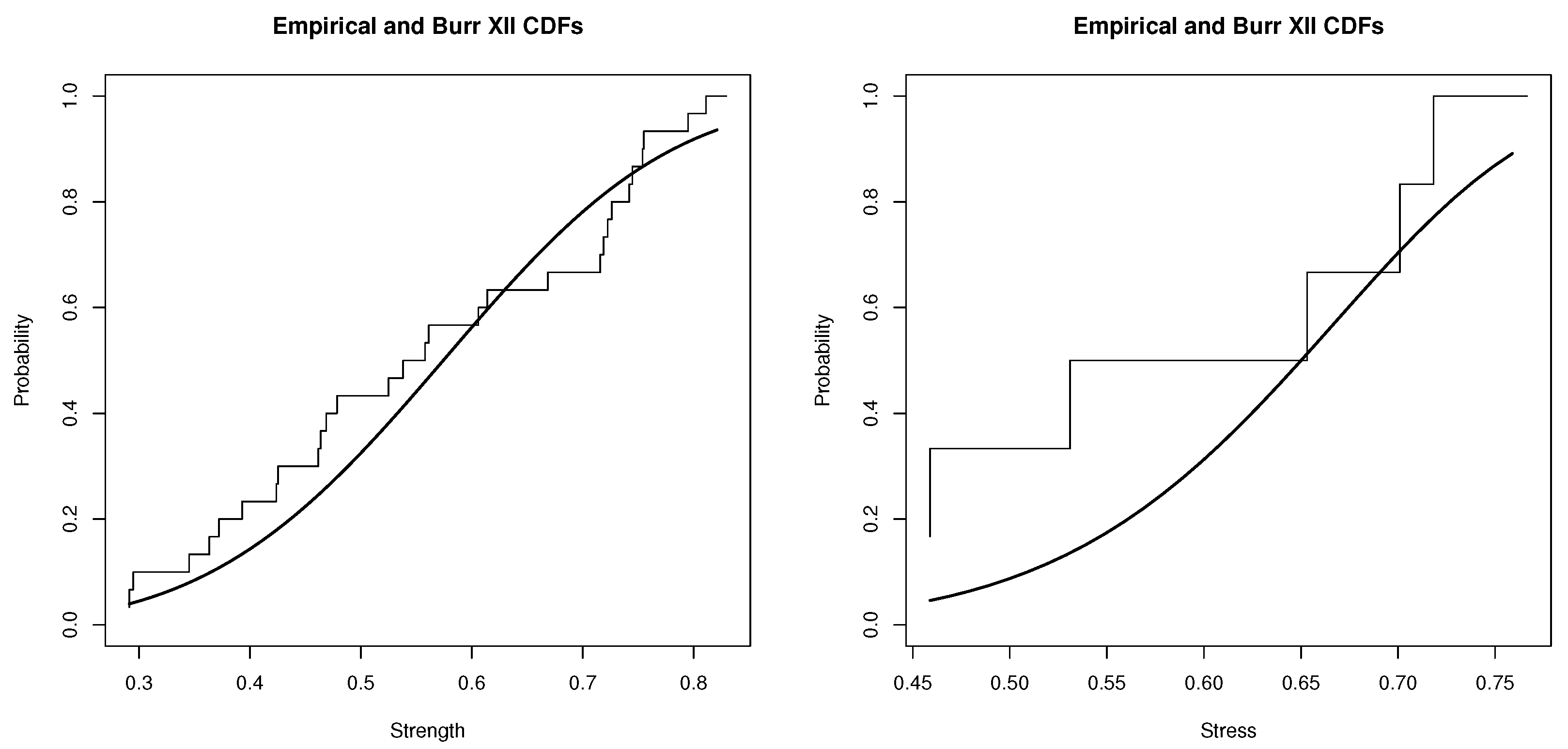
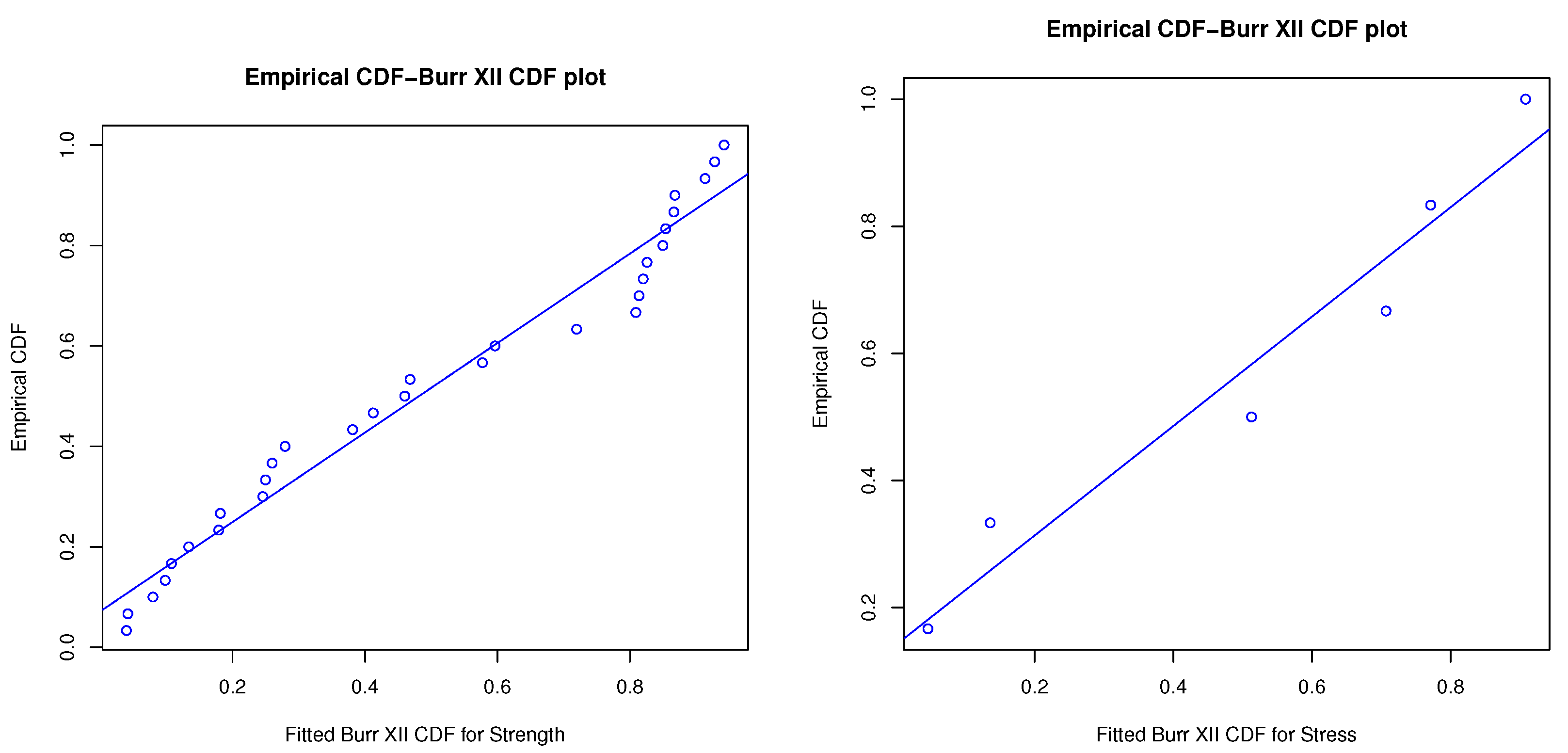
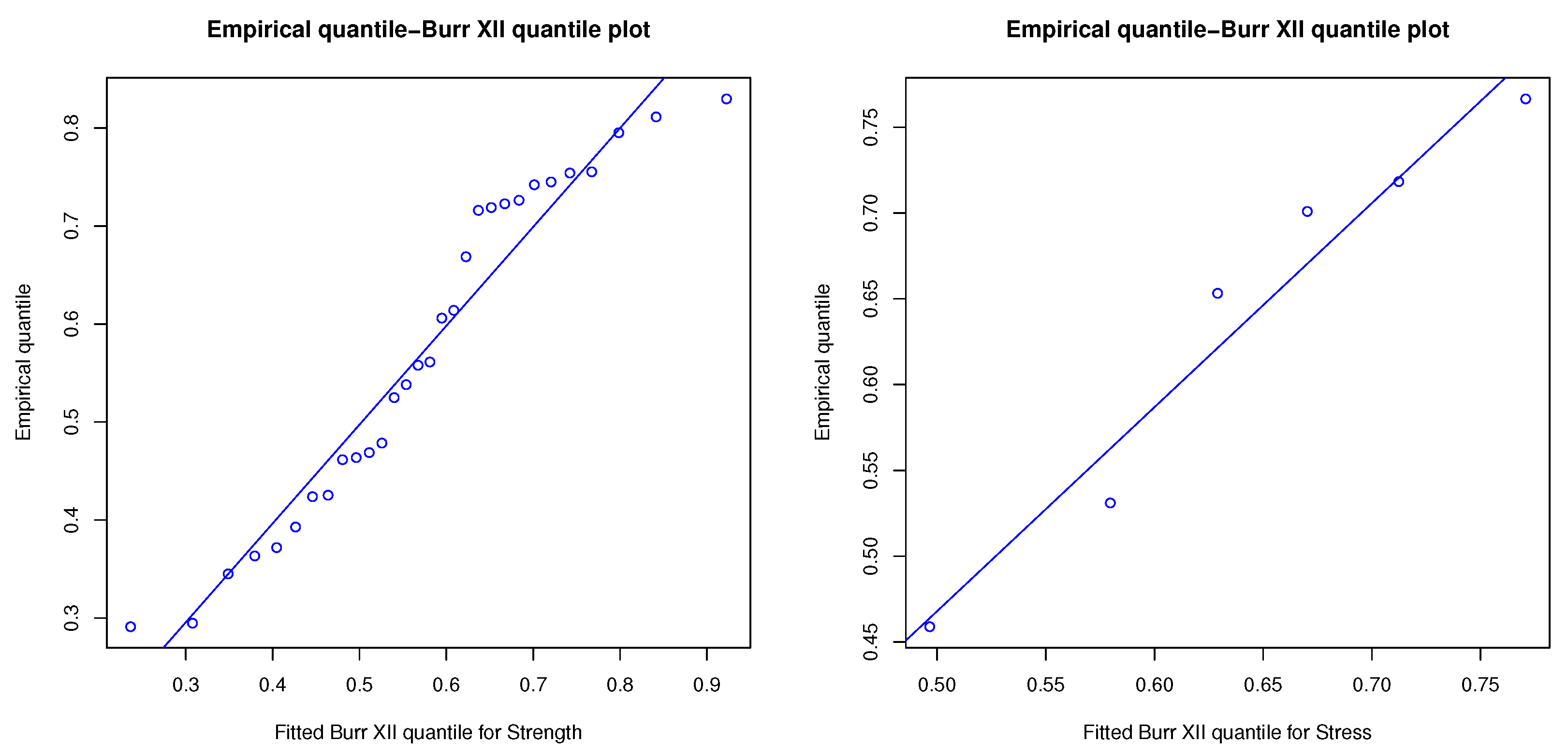
The Burr XII distribution is applied to fit these real-life data via using the Kolmogorov–Smirnov (K–S) test with two-sided reject region. The results for strength and stress data have distances and the corresponding p-values (within brackets), $0.17557\left(0.2793\right)$ and $0.20679\left(0.9158\right)$, respectively. Additionally, the plots of empirical cumulative and Burr XII distributions overlay. Probability–probability (P–P) and Quantile–Quantile (Q–Q) plots are shown in Figure 1, Figure 2 and Figure 3. P–P plot is a probability plot for evaluating how closely of a dataset fitting a specified model or how closely two datasets agree. Q-Q plot is a graphic method for evaluating if two datasets come from populations with a common distribution. Figure 2 shows two P-P plots to present the empirical CDFs of the strength (left side) and the stress (right side) versus the theoretical CDF of Burr XII. The imposed linear regressions over P-P plots in Figure 2 are significant with R-squared, 0.9664 and 0.9459, for the complete strength and stress samples, respectively and the imposed linear regressions over Q-Q plots in Figure 3 are also significant with R-squared, 0.9461 and 0.9502, for the complete strength and stress samples, respectively. Therefore, the Burr XII distribution can be used as a proper probability model to address the transformed datasets well.

Based on previous complete strength and stress data, a MSR censored observation of the 3-out-of-5 G system can be constructed as

$$\begin{array}{c}\hfill \begin{array}{ccc}\mathrm{Strength}\mathrm{data}\mathrm{of}X& & \mathrm{Stress}\mathrm{data}\mathrm{of}Y\\ \left(\begin{array}{ccc}0.4238& 0.5579& 0.7262\\ 0.2912& 0.3634& 0.3719\\ 0.5381& 0.5612& 0.7226\\ 0.5249& 0.6060& 0.6686\\ 0.3451& 0.4253& 0.4688\\ 0.2948& 0.3929& 0.4616\end{array}\right)& \mathrm{and}& \left(\begin{array}{c}0.7009\\ 0.6532\\ 0.4589\\ 0.7183\\ 0.5310\\ 0.7665\end{array}\right).\end{array}\end{array}$$

The associated point and interval estimates for the MSR parameter $R_{s,k}$ are presented in

Table 6. The estimates of $R_{s,k}$ based on the real dataset from 3-out-of-5 G System.

${\lambda }_1={\lambda }_2$
${\widehat{\mathit{R}}}_{\mathit{s},\mathit{k}}=\mathbf{0.4792}$	${\acute{\mathit{R}}}_{\mathit{s},\mathit{k}}=\mathbf{0.4451}$	${\acute{\mathit{R}}}_{\mathit{s},\mathit{k}}^{\mathit{F}}=\mathbf{0.4556}$
ACI$=(0.3169,0.7246)$	GCI$=(0.1989,0.6938)$	BCI$=(0.2076,0.8153)$
${\lambda }_1\ne {\lambda }_2$
${\check{\mathit{R}}}_{\mathit{s},\mathit{k}}=\mathbf{0.3403}$	${\stackrel{`}{\mathit{R}}}_{\mathit{s},\mathit{k}}=\mathbf{0.4133}$	${\stackrel{`}{\mathit{R}}}_{\mathit{s},\mathit{k}}^{\mathit{F}}=\mathbf{0.4244}$
ACI$=(0.2029,0.5707)$	GCI$=(0.1416,0.6605)$	BCI$=(0.0639,0.6430)$

, where the significance level of $\gamma$ is taken to be $0.05$. The interval lengths are obtained as 0.4077, 0.4949 and 0.6077 for the ACI, GCI and BCI, respectively, under ${\lambda }_1={\lambda }_2$ and as 0.3678, 0.5189 and 0.5791 for ACI, GCI and BCI, respectively, under ${\lambda }_1\ne {\lambda }_2$. It is observed that the point estimates are close to each other and the ACI of $R_{s,k}$ performs better than the others in terms of interval length.

Furthermore, for comparison of the equivalence between strength and stress inner shape parameters, ${\lambda }_1$ and ${\lambda }_2$, the likelihood ratio statistic and p-value are calculated as $3.5068$ and $0.0611$, respectively. The results show that there is no significant statistical evidence to reject the null hypothesis, $H_0:{\lambda }_1={\lambda }_2$ at 0.05 significance level. Hence, the strength and stress are suggested to have Burr XII distributions with equal inner shape parameter ${\lambda }_1$ and ${\lambda }_2$ for this current monthly capacity data application.

7. Concluding Remarks

The reliability inference for a multicomponent stress–strength model has been studied based on the Burr XII distributions. The existence and uniqueness of maximum likelihood estimators of the strength and stress parameters are established and the generalized pivotal quantity-based estimators have been constructed under common and unequal inner shape parameter situations. Meanwhile, confidence intervals have also been provided using asymptotic normal distribution along with delta technique, bootstrap percentile and generalized pivotal sampling, respectively. Generally, simulation results show that bootstrap percentile procedure produces better ACI than the other two in terms of coverage probability for all cases. When two inner shape parameters are equal, asymptotic normal distribution along with delta method and generalized pivotal sampling are very competitive with each other in terms of coverage probability. However, the maximum likelihood method provides better point estimators than the generalized pivotal sampling method in terms of MSE and AB. Overall, the proposed procedures work quite well under the given sampling scheme, except for the ACI based on delta method for the case of unequal inner shape parameters.

Although the current work is developed using a Type-II censoring scheme, it can be extended to other censoring schemes such as the progressively Type-II censoring scheme or progressively first-failure Type-II censoring scheme with proper modification of pivotal quantities for the progressively Type-II or progressively first-failure Type-II censored samples. For further study, the moment estimation and the maximum product of spacing estimation seem also interesting to pursue new inferential results and will be discussed in future. The authors are currently working on these possible projects.

References

- Eryilmaz, S. Phase type stress-strength models with reliability applications. Commun.-Stat.-Simul. Comput. 2018, 47, 954–963. [Google Scholar] [CrossRef]
- Kundu, D.; Kundu, D. Estimation of R = P(Y < X) for three-parameter Weibull distribution. Stat. Prob. Lett. 2009, 79, 1839–1846. [Google Scholar]
- Krishnamoorthy, K.; Lin, Y. Confdence limits for stress-strength reliability involving Weibull models. J. Stat. Plan. Inference 2010, 140, 1754–1764. [Google Scholar] [CrossRef]
- Mokhlis, N.A.; Ibrahim, E.J.; Ibrahim, E.J. Stress-strength reliability with general form distributions. Commun.-Stat.-Theory Methods 2017, 46, 1230–1246. [Google Scholar] [CrossRef]
- Wang, B.; Geng, Y.; Zhou, J. Inference for the generalized exponential stress-strength model. Appl. Math. Model. 2018, 53, 267–275. [Google Scholar] [CrossRef]
- Bhattacharyya, G.K.; Johnson, R.A. Estimation of reliability in multicomponent stresss-trength model. J. Am. Stat. Assoc. 1974, 69, 966–970. [Google Scholar] [CrossRef]
- Dey, S.; Mazucheli, J.; Anis, M.Z. Estimation of reliability of multicomponent stress-strength for a Kumaraswamy distribution. Commun.-Stat.-Theory Methods 2017, 46, 1560–1572. [Google Scholar] [CrossRef]
- Kayal, T.; Tripathi, Y.M.; Dey, S.; Wu, S.J. On estimating the reliability in a multicomponent stress-strength model based on Chen distribution. Commun.-Stat.-Theory Methods 2020, 49, 2429–2447. [Google Scholar] [CrossRef]
- Kizilaslan, F. Classical and Bayesian estimation of reliability in a multicomponent stress-strength model based on a general class of inverse exponentiated distributions. Stat. Pap. 2018, 59, 1161–1192. [Google Scholar] [CrossRef]
- Kizilaslan, F. Classical and Bayesian estimation of reliability in a multicomponent stress-strength model based on the proportional reversed hazard rate model. Math. Comput. Sim. 2017, 136, 36–62. [Google Scholar] [CrossRef]
- Kizilaslan, F.; Nadar, M. Estimation of reliability in a multicomponent stress-strength model based on a bivariate Kumaraswamy distribution. Stat. Pap. 2018, 59, 307–340. [Google Scholar] [CrossRef]
- Nadar, M.; Kizilaslan, F. Estimation of reliability in a multicomponent stress-strength model based on a Marshall-Olkin bivariate Weibull distribution. IEEE Trans. Reliab. 2016, 65, 370–380. [Google Scholar] [CrossRef]
- Rao, G.S. Estimation of reliability in multicomponent stress-strength model based on Rayleigh distribution. ProbStat. Forum. 2012, 5, 150–161. [Google Scholar]
- Rao, G.S.; Aslam, M.; Kundu, D. Burr type XII distribution parametric estimation and estimation of reliability of multicomponent stress-strength. Commun.-Stat.-Theory Methods 2015, 44, 4953–4961. [Google Scholar] [CrossRef]
- Sauer, L.; Lio, Y.; Tsai, T.-R. Reliability inference for the multicomponent system based on progressively type II censoring samples from generalized Pareto distributions. J. Math. 2020, 8, 8071176. [Google Scholar]
- Wang, L.; Lin, H.; Ahmadi, K.; Lio, Y. Estimation of stress-strength reliability for multicomponent system with Rayleigh data. J. Energies 2021, 14, 7917. [Google Scholar] [CrossRef]
- Burr, I.W. Cumulative frequency functions. Ann. Math. Stat. 1946, 13, 215–232. [Google Scholar] [CrossRef]
- Tadikamalla, P.R. A look at the Burr and related distributions. Int. Stat. Rev. 1980, 48, 337–344. [Google Scholar] [CrossRef]
- Kumar, D. The Burr type XII distribution with some statistical properties. J. Data Sci. 2017, 16, 509–534. [Google Scholar] [CrossRef]
- Lio, Y.L.; Tsai, T.-R. Estimation of δ = P(X < Y) for Burr XII distribution based on the progressively first failure-censored samples. J. Appl. Stat. 2012, 39, 309–322. [Google Scholar]
- Wingo, D.R. Maximum likelihood methods for fitting the Burr type XII distribution to life test data. Biom. J. 1983, 25, 77–84. [Google Scholar] [CrossRef]
- Wingo, D.R. Maximum likelihood methods for fitting the Burr type XII distribution to multiply (progressively) censored life test data. Metrika 1993, 40, 203–210. [Google Scholar] [CrossRef]
- Wu, J.W.; Yu, H.Y. Statistical inference about the shape parameter of the Burr type XII distribution under the failure-censored sampling plan. Appl. Math. Comput. 2005, 163, 443–482. [Google Scholar] [CrossRef]
- Zimmer, W.J.; Keats, J.B.; Wang, F.K. The Burr XII distribution in reliability analysis. J. Qual. Technol. 1998, 30, 386–394. [Google Scholar] [CrossRef]
- Efron, B. The Jackknife, the Bootstrap, and Other Resampling Plans, CBMSNSF Regional Conference Series in Applied Mathematics; SIAM: Philadelphia, PA, USA, 1982; Volume 38. [Google Scholar]
- Hall, P. Theoretical comparison of bootstrap confidence intervals. Ann. Stat. 1988, 16, 927–953. [Google Scholar] [CrossRef]
- Weerahandi, S. Generalized Inference in Repeated Measures: Exact Methods in MANOVA and Mixed Models; Wiley: New York, NY, USA, 2004. [Google Scholar]
- Xu, J.; Long, J.S. Using the Delta Method to Construct Confidence Intervals for Predicted Probabilities, Rates, and Discrete Changes; Lecture Notes; Indiana University: Bloomington, IN, USA, 2005. [Google Scholar]
- Lawless, J.F. Statistical Models and Methods for Lifetime Data, 2nd ed.; Wiley: New York, NY, USA, 2003. [Google Scholar]
- Stephens, M.A. Tests for the exponential distribution. In Goodness-of-Fit Techniques; D’Agostino, R.B., Stephens, M.A., Eds.; Marcel Dekker: New York, NY, USA, 1986; pp. 421–459. [Google Scholar]
- Viveros, R.; Balakrishnan, N. Interval estimation of parameters of life from progressively censored data. Technometrics 1994, 36, 84–91. [Google Scholar] [CrossRef]
Figure 1.
Empirical and fitted Burr XII distributions based on real data.
Figure 2.
Probability to probability plot based on real data.
Figure 3.
Quantity to quantity plots based on real data.