
A Neural Network Model Secret-Sharing Scheme with Multiple Weights for Progressive Recovery


1
College of Electronic Engineering, National University of Defense Technology, Hefei 230037, China
2
Anhui Key Laboratory of Cyberspace Security Situation Awareness and Evaluation, Hefei 230037, China
*
Author to whom correspondence should be addressed.
Mathematics 2022, 10(13), 2231; https://doi.org/10.3390/math10132231
Submission received: 18 May 2022
/
Revised: 18 June 2022
/
Accepted: 21 June 2022
/
Published: 25 June 2022
(This article belongs to the Special Issue Frontiers in Mathematical Methods of Secret Sharing and Applied Cryptography)
Abstract
:With the widespread use of deep-learning models in production environments, the value of deep-learning models has become more prominent. The key issues are the rights of the model trainers and the security of the specific scenarios using the models. In the commercial domain, consumers pay different fees and have access to different levels of services. Therefore, dividing the model into several shadow models with multiple weights is necessary. When holders want to use the model, they can recover the model whose performance corresponds to the number and weights of the collected shadow models so that access to the model can be controlled progressively, i.e., progressive recovery is significant. This paper proposes a neural network model secret sharing scheme (NNSS) with multiple weights for progressive recovery. The scheme uses Shamir’s polynomial to control model parameters’ sharing and embedding phase, which in turn enables hierarchical performance control in the secret model recovery phase. First, the important model parameters are extracted. Then, effective shadow parameters are assigned based on the holders’ weights in the sharing phase, and t shadow models are generated. The holders can obtain a sufficient number of shadow parameters for recovering the secret parameters with a certain probability during the recovery phase. As the number of shadow models obtained increases, the probability becomes larger, while the performance of the extracted models is related to the participants’ weights in the recovery phase. The probability is proportional to the number and weights of the shadow models obtained in the recovery phase, and the probability of the successful recovery of the shadow parameters is 1 when all t shadow models are obtained, i.e., the performance of the reconstruction model can reach the performance of the secret model. A series of experiments conducted on VGG19 verify the effectiveness of the scheme.
MSC:
94A62; 68T071. Introduction
In recent years, deep learning has achieved amazing results in computer vision [1,2,3], speech recognition [4,5], natural language processing [6,7,8], bioinformatics [9,10], and other fields. Trained deep-learning models are highly valuable. There have been numerous attacks against the intellectual property of models using methods such as building detectors to attack ownership verification and thus obtain the model [11]. Malicious users who obtain models may illegally copy and redistribute them or use them to provide services without permission. In addition, in the commercial domain, different levels of consumers have different permissions. Therefore, it is necessary to control permission to use the models.
Many model-permission control strategies are proposed for this purpose. Digital watermarking is a technology that hides specific information in a digital cover and can confirm the ownership of a cover after piracy. Neural network digital watermarking is the permission-control strategy that has received the most attention from researchers. Zhang et al. [12] enable the neural network to learn a specific pattern by changing the label and establishing a correspondence between the specific pattern and the changed label. By adding a regularization term for the associated watermark, Wang et al. [13] enable the neural network to automatically embed the watermark in the model parameters during the training phase. Encryption of the model is different from digital watermarking, which can verify the visitor’s authority when using the model. In general, the straightforward strategy for encrypting a model is to encrypt all model parameters by traditional encryption methods such as RSA [14], AES [15] and so on. For resource-constrained devices, encryption and decryption are very expensive, so some schemes use a selection strategy to encrypt some of the parameters in the model. Tian et al. [16] propose a probabilistic selection strategy (PSS) to determine the importance of parameters in convolutional neural networks (CNN) and protect CNN by encrypting important parameters. Chen and Wu [17] propose a novel framework for deep-learning models that provides access control to the trained deep neural networks so that only authorized users can utilize them properly.
Although both digital watermarking and encryption can protect deep-learning models, neither enables permission control over the co-trained models in the federation. They also do not enable progressive recovery of models and control over the weights of participants. For these reasons, we need to apply secret sharing (SS) to the permission-control scheme of the models. SS is a data-protection technology that divides a secret into several shadows and shares them to different participants [18,19]. Only the participants that satisfy the conditions can recover the original secret information. Compared with information hiding, SS has the property of loss tolerance. The SS technique is of great value in permission control and identity authentication.
Participants in most SS-based schemes have the same weight. However, in some scenarios, some participants need to be given different weights to indicate thei importance compared with other participants. Hou et al. [20] proposed a permission-based visual secret-sharing (VSS) scheme where the participants of a scheme have the same image size and different weights. In the recovery phase, the greater the participants’ weight, the better the quality of the recovered images. However, the recovered images in their scheme are lossy. Liu et al. [21] proposed the threshold for random-lattice VSS which provides both OR and XOR recovery. It has the property of lossless recovery in XOR recovery.
Participants contribute differently to the generated model, so they should have different abilities to recover the model if the model is protected. Different fees are paid in the process of upgrading the model by the consumer, and the corresponding degree of performance upgrade varies. This feature is not yet possible with the current research on the permission protection of models.
This paper proposes a threshold neural network model secret-sharing (NNSS) scheme with multiple weights for progressive recovery. The model parameters are encrypted using Shamir’s secret sharing (SSS) and control of the embedding process of shadow parameters to achieve hierarchical performance control in the recovery phase. The results achieved by the scheme proposed in this paper are shown to be as follows.
The performance of the reconstructed model starts to improve when the number of participants in the recovery phase reaches k; the performance of the reconstructed model can be comparable to that of the secret model when the number of participants reaches t. Meanwhile, the performance of the reconstructed model is related to the weights of participants.
2. Related Works
In the scheme of this paper, Shamir’s secret-sharing scheme embeds the secret parameters into the shadow parameters. The weighted polynomial-based secret-image sharing scheme achieves the property that the probability of the successful recovery of secret parameters is positively correlated with the participants’ weights. The probabilistic selection strategy (PSS) can select the part of the parameters that have an enormous impact on the model performance. SS only, for this part of the parameters, can reduce the computational effort of the sharing phase. The above work is presented in this section.
2.1. Shamir’s Secret-Sharing Scheme
Shamir [18] proposed a scheme capable of partitioning one secret into n shadows, and the secret can be reconstructed if k number of shadows or more are gained. For n participants in the sharing phase, each participant holds an integer x. The shadow held by this participant can be computed by substituting x into a polynomial as shown in Equation (1):
The reconstruction secret is based on a Lagrange interpolation formula as shown in Equation (2). The integers and the shadows held by the k participants of the recovery phase are substituted into the formula to calculate the secret, i.e., the constant term of the computed formula.
2.2. Weighted Polynomial-Based Secret-Image Sharing Scheme
Secret-image sharing (SIS) is an application of the SS technique in the image domain [22], where each pixel point is treated as a secret and shared as n shadow pixels by a Shamir polynomial. The secret image can be reconstructed only if at least k shadow images are gained. Wang’s proposed weighted polynomial-based SIS scheme [23] uses polynomial SIS based on a threshold to generate k shadow images and assign corresponding weights to them. Then, the remaining shares are filled with invalid values. When the threshold is satisfied, the number of shares and the weights affect the quality of the reconstructed images. The image can be recovered losslessly when all participants are involved in the recovery phase. Wang proposed the definition of the correct recovery probability (CRP) to measure the quality of the reconstructed image. CRP is the ratio of the number of identical pixels in the same position between the reconstructed image and the secret image to the total number of pixels. The larger the CRP value, the higher the quality of the reconstructed image. The NNSS scheme proposed in this paper is closer to this scheme regarding ideas. It is considered that the more the number of identical parameters at the same position between the reconstructed model and the secret model, the closer the performance of the reconstructed model is to that of the secret model.
For a secret image S of size , the CRP of its reconstructed image is calculated as shown in Equation (3).
T is the number of identical pixels at the same position in both images.
2.3. Probabilistic Selection Strategy
Tian et al. [16] proposed PSS to select the important parameters from the convolutional layer parameters of CNN. Many studies [24,25,26,27] have shown that the parameters in CNNs are not of equal importance, so the performance of CNNs can be controlled by selecting a small number of more important parameters. The specific principle of PSS is as follows. represents the parameters of the l-th layer. When changing the inputs of the training instances, for each input instance, a subset exists, and the performance of the pre-trained model degrades the most when the subset does not exist. The probability that the parameter appears in represents the importance of the parameter. They describe this problem as an optimization problem, as shown in Equation (4).
where I represents a vector of equal length to , represents a sample of the binary random variable , and is a weighting factor for the regularization term.
3. The Proposed Scheme
3.1. Motivation
Deep-learning models face many threats. For example, Oracle [28], by which an attacker can study the relationship between input and output and use these results to gain training data; poisoning, by which an attacker can modify the behavior of a machine-learning algorithm through modified data or models; adversarial attack, model or data disclosure, and so on. Threats such as Oracle and model disclosure can be addressed by controlling access to the model. Taking the Oracle as an example, if only legitimate visitors can access the model, then the attacker cannot obtain the input–output pairs. Therefore, permission control of the model is significant.
Many studies exist for permission control of deep-learning models, including adding watermarks to the models and encrypting the models. Watermarks can verify ownership of the model when illegal access to the model is detected [12]; encrypting a model can prevent illegal access to the model. However, none of these can realize the permission control of the jointly trained models in the federation; meanwhile, different participants have different importances in some permission-control application scenarios with multiple participants. Thus, the different shadow models should have different abilities to recover the secret models. Most of the current model-encryption schemes generate only one copy of the encrypted model [15], which the model cannot recover after loss or error, and thus cannot achieve loss tolerance. Although PSS enables hierarchical control of model performance, it does not enable progressive performance recovery during the recovery phase.
Therefore, a multi-weight model-permission-control scheme for progressive-recovery characteristics that can realize the federated permission control is of some significance.
3.2. NNSS with Multiple Weights for Progressive Recovery
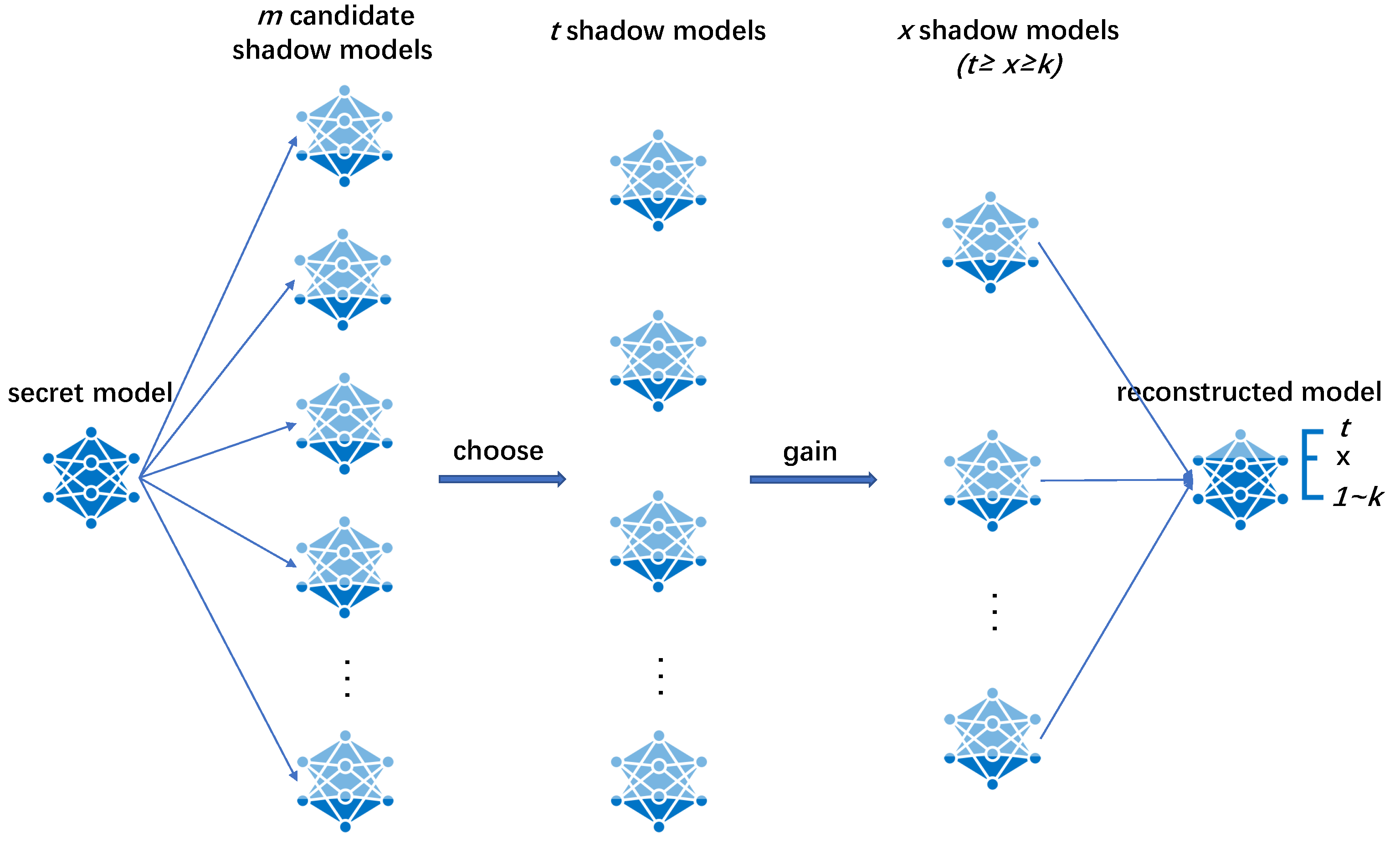
In this paper, we propose a threshold NNSS with multiple weights for progressive recovery, which works as follows. In the sharing phase, shadow models are generated based on the secret model and assign t of them to t participants. Each shadow model held by each participant has the same performance. The performance of the shadow models is the initial performance for recovering the model during the recovery phase. In the recovery phase, at least k participants exist to recover the model. The performance of the reconstructed model is related to the weights and number of participants. When the number of participants reaches t, the performance of the reconstructed model can be comparable to that of the secret model. The workflow diagram of the NNSS scheme proposed in this paper is shown in Figure 1, where the dark blue area of the model represents its performance.
3.2.1. Sharing Phase
- Calculate . m is the number of candidate shadow models. m is calculated based on the following. When obtaining t shadow models, the secret parameters can be recovered by t shadow parameters at any position of the model. In other words, even if t shadow parameters contain all invalid parameters, there are at least k valid parameters, i.e., .Next, m candidate shadow models are generated, from which t models are selected and assigned to t participants. Each participant has exactly one shadow model.
- According to the scenario, weights are assigned to the m candidate shadow models. The size of the weights is set manually. Generally, the shadow models held by the participants with the least important weight and the excess shadow models are assigned as 1. The weights of other shadow models are assigned a number greater than 1 according to their importance difference. The importance of the shadow model can be measured by the participant’s contribution to the model training process, such as the amount of data provided, the number of CPU operations provided, etc.
- Determine the SS phase’s finite domain . Assign m candidate secret models with mutually different m integers in the finite domain to generate shadow parameters.
- Use PSS to extract important parameters of the secret model.
- Convert important parameters to integers in a finite field. It is well-known that traditional SS is for non-negative integers. However, the parameters in the secret model are floating-point numbers, so consider transforming floating-point numbers into a finite field for SSS. is the set of parameters for the deep-learning model. Floating-point numbers are converted to non-negative integer space by Equation (5):The larger U is the more decimal places the parameters retain, and the higher the accuracy of the parameters of the reconstructed model. However, the converted integer must be in , so U must satisfy . Thus, this paper calculates the specific value of U by Equation (6).
- Iterate through the generated integers. Perform the -threshold SSS for each integer using polynomials to generate n integers in a finite field. These n integers are called valid integers In addition, generate invalid integers . can be calculated by Equations (7).where H is a positive integer and P is the number of finite field features in Equation (1).
- Assign integers based on the candidate-shadow-model weights. The higher the weight of the candidate shadow model, the easier it is to assign a valid integer. The details of this operation are shown in Algorithm 1.
Algorithm 1 Assign integers based on the candidate shadow model weights. - Require:
- The number of candidate shadow models m, the number of effective shadows n, list of weights of candidate shadow models , set of valid integers, set of invalid integers
- Ensure:
- allocation of integers
- 1:
- while There are valid integers that have not been assigned do
- 2:
- 3:
- Generate empty list
- 4:
- while to m do
- 5:
- 6:
- Append t to
- 7:
- end while
- 8:
- Generate a random number in (0,1)
- 9:
- 10:
- while to m do
- 11:
- if then
- 12:
- 13:
- Stop the loop
- 14:
- end if
- 15:
- end while
- 16:
- Take any valid integer and assign it to the candidate shadow model with index.
- 17:
- 18:
- end while
- 19:
- Randomly assign invalid integers to candidate shadow models that have not yet been assigned.
This step enables the recovery phase to acquire with a certain probability a sufficient number of shadow parameters used to recover the secret parameters. As the number of shadow models acquired increases, the probability becomes larger. When all t shadow models are gained, the reconstructed model has the performance of the secret model. The performance of the extracted models is related to the participants’ weights in the recovery phase. Now, each important parameter selected corresponds to m integers that have been assigned to the candidate shadow model. - Embed integers into candidate shadow models. Each candidate shadow model takes a copy of the secret model as its initial state. Fill the generated shadow parameter to the corresponding positions of their corresponding candidate shadow model by solving the system of equations shown in Equation (8) for each integer. Finally, m copies of the candidate shadow models are generated. Select t of these candidate shadow models to assign to t participants based on their weights, with each participant having exactly one copy of the shadow model.where I is the integer currently being processed, and p is the secret parameter at the corresponding location. H corresponds to the eponymous parameter in the system of Equation (7). represents the deviation that determines both the performance of the participant’s shadow model and the reconstructed model’s starting performance. R is the precision that controls the precision of the effect of on performance.
3.2.2. The Recovery Phase
The recovery of the reconstructed model can be started when there are at least k participants in the recovery phase.
- Select any shadow model as the initial state of the reconstructed model.
- Iterate through the positions of all model parameters. It is skipped if all the shadow models have the same parameters at the current position. Otherwise, it means that the parameters of the shadow models at the current position hide the shadow parameters. At this time, the integers I are extracted from parameter p of the shadow model at the current position by Equation (9).where R and H mean the same as they do in Equation (8).When the number of valid integers in the extracted integers is k or more, the Lagrangian interpolation formula, as shown in Equation (2), is used to recover the integers x corresponding to the secret parameter at the current position. Then, x is converted to the secret parameter by Equation (10) and filled to the corresponding positions in the reconstructed model.where U and mean the same as they do in Equation (5).The corresponding parameter of any of the shadow models is selected to fill the corresponding position of the reconstructed model when the number of valid integers among the extracted integers is less than k.
3.3. Validity Analyses
We consider that if a reconstructed model has more of the same number of parameters as the secret model at the corresponding position, its performance is closer to the secret model. For any location where the secret parameter is hidden, the parameter of the secret model can definitely be obtained in the recovery phase when the number of valid integers extracted, j, is more than k. Thus, the probability of (i.e., ) in a sharing state which is determined by the weights of the m candidate shadow models, and the weights of the t selected shadow models, can reflect the performance of the reconstructed model.
Based on the above, this subsection attempts to calculate and analyze this scheme’s progressivity and weight validity.
3.3.1. Progressivity Analyses
In the scheme proposed in this paper, progressivity means that the more secret model involved in the recovery, the better the performance of the reconstructed model. We need to calculate the variation of as x is changed when x shadow models are randomly selected from t candidate shadow models to participate in the recovery phase at a determined sharing state, and the progressivity is analyzed accordingly.
There are two points to note in the analyses.
- The expected performance of the reconstructed model at a certain x needs to be considered to measure progressivity. Therefore, x shadow models are chosen randomly.
- is for a location where the secret parameter is hidden, not for the whole recovery phase. Considering the huge number of parameters, there must be the case where in the whole recovery phase.
For the -threshold NNSS with multiple weights for progressive recovery, when as, even if t shadow models contains all invalid integers, there are valid integers remaining.
Consider the more general case, i.e., the value of when x is a variable. The calculation procedure is as follows.
- Calculate the probability of the combination of all candidate shadow models with getting valid integers in one process of assigning n valid integers to m candidate shadow models, i.e.,There are different valid integer-assignment orders for each . The probability of each assignment order is not the same. is equal to the sum of the probabilities of all assignment orders, and its solution algorithm is shown in Algorithm 2.
Algorithm 2 Solution for the probability of the combination of all candidate shadow models with obtaining valid integers. - Require:
- , the list of participants’ weights W
- Ensure:
- 1:
- Compute all possible full permutations of and their combination is called .
- 2:
- Initialize .
- 3:
- while There are still unretrieved permutations in . do
- 4:
- Take any of the permutations a in
- 5:
- Reset W
- 6:
- 7:
- while There are still unretrieved model number indexs in a do
- 8:
- Find the smallest index in a
- 9:
- Calculate the probability list according to W
- 10:
- 11:
- 12:
- end while
- 13:
- 14:
- end while
- t shadow models are selected from m candidate shadow models according to their weights, and their combination is . Since the number of valid integers in is related to both and , but is a constant for the entire the recovery phase, it is determined after all important model parameters have been shared. Let the number of valid integers contained in be during a certain parameter sharing phase. Consider the number j of valid integers extracted at any one location when x shadow models are randomly selected from . The range of values of j is [,]. Where means that all invalid integers in are included in the x person selected at the current position. At determination, the probability is as shown in Equation (11) for each value j taken.where denotes the number of cases in which any j integers are selected from all valid integers of . Furthermore, denotes the number of cases in which any integers are selected from all invalid integers of . In addition, denotes the number of cases in which any x integers are selected from .
- when x is a variable is shown in Equation (12).where S represents the combination of all possible cases of .
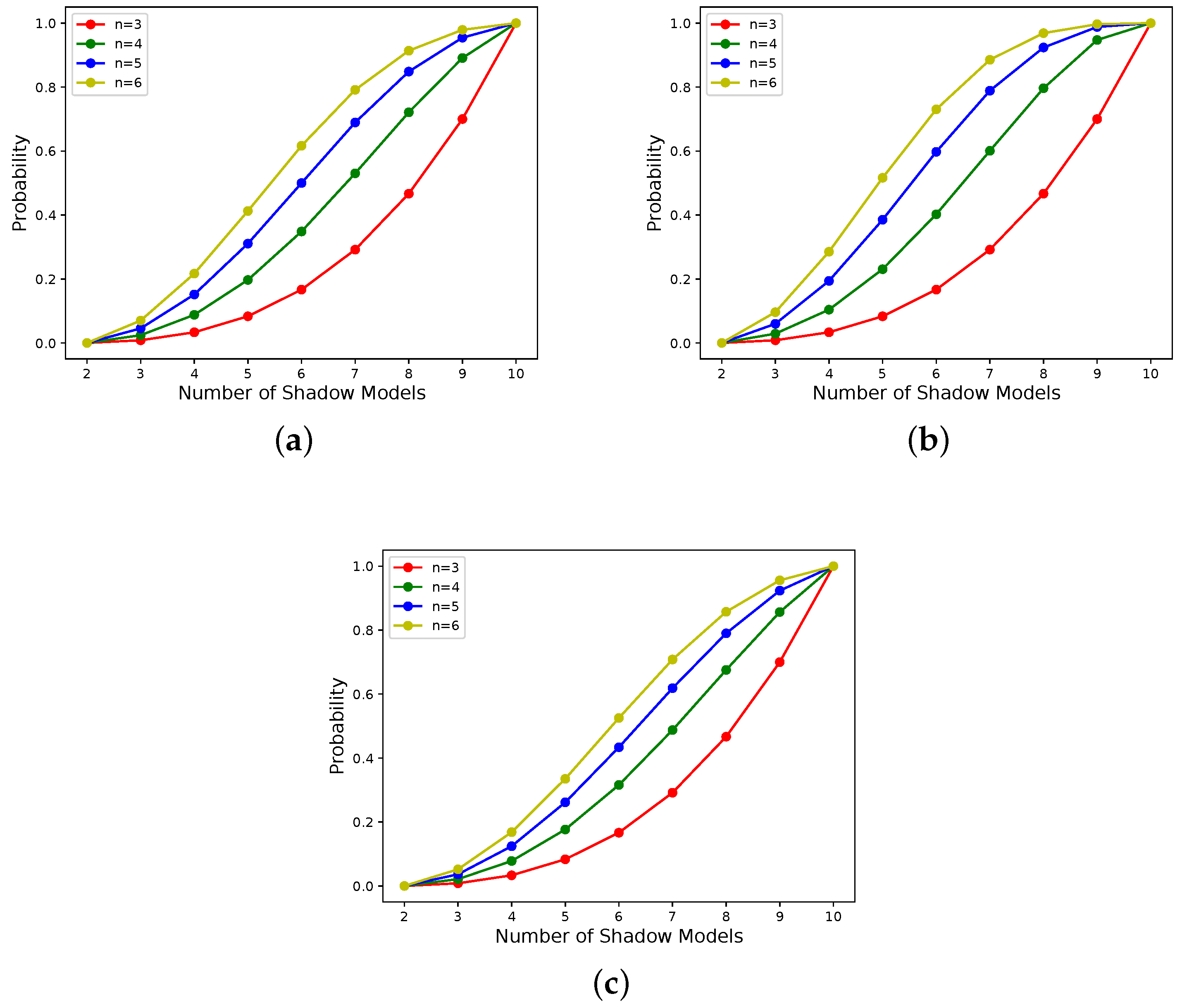
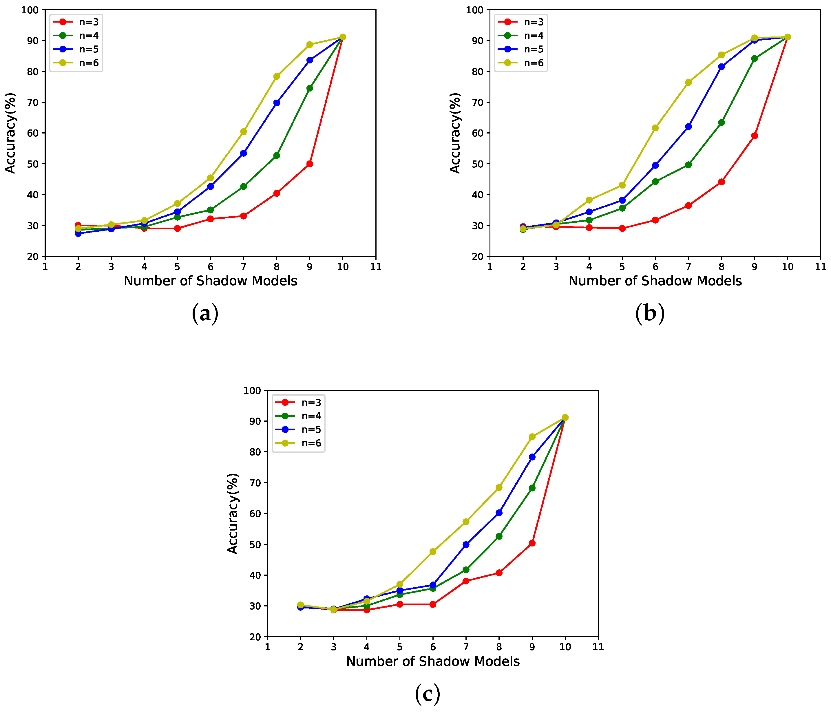
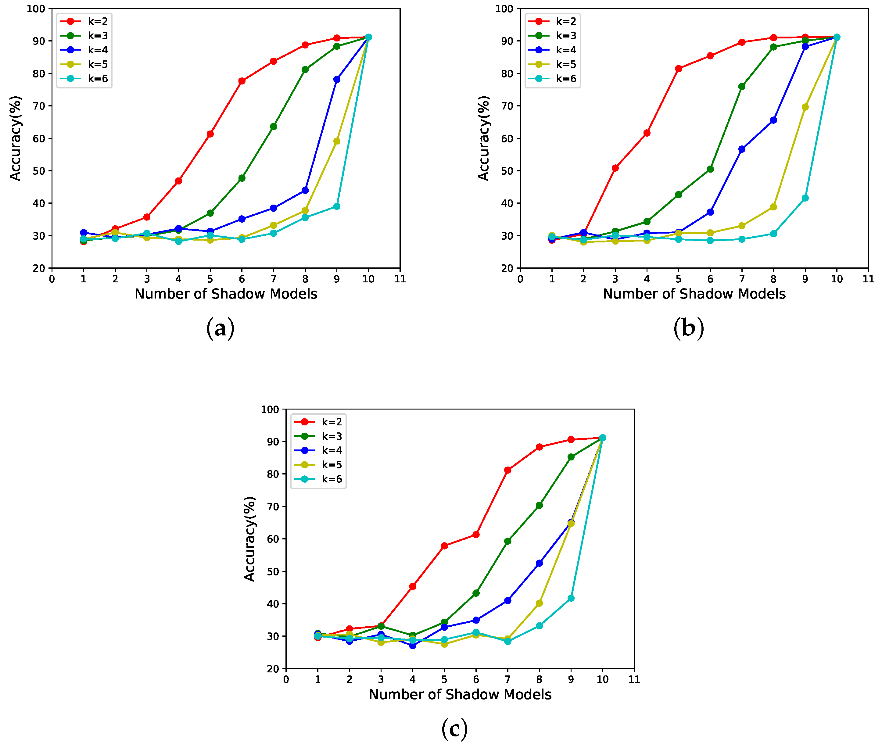
With n in [3, 6] and x in [2, 10] for the -threshold NNSS, the relationship between x and for different determined sharing states is shown in Figure 2. With k in [2, 6] and x in [1, 10] for the -threshold NNSS, the relationship between x and for different determined sharing states is shown in Figure 3. The correspondence between the subgraph, candidate-shadow-model weights and shadow-model weights is shown in Table 1.
The above results show that the proposed scheme is feasible in progressivity. Its progressive effect is inferred as follows.
When , it is impossible to reconstruct a model with better performance than the shadow model. When , the reconstructed model can have the performance of the secret model. When k and t are determined, the corresponding to different x increases in different magnitudes as n increases, and when n and t are determined, the corresponding to different x decreases in different magnitudes as k increases, which has an impact on the progressivity of model recovery. Specifically, when , the progressivity exists but is not significant in the case of a small number of x. As n increases, the progressivity becomes more pronounced for a smaller number of x. The progressivity becomes less pronounced for a larger number of x. As k increases, the progressivity becomes more pronounced for a larger number of x. The progressivity becomes less pronounced for a smaller number of x.
3.3.2. Weight Validity Analyses
In the proposed scheme, weight validity means that the larger the weight of the people involved in the recovery phase, the better the performance of the reconstructed model when the number x of secret models is selected from t secret models is constant in a determined sharing situation. Therefore, we need to calculate for weight validity analyses when selecting specific x shadow models from t secret models, which is different from randomly selecting x shadow models when analyzing progressivity. Then the selected x secret models are changed without changing the current sharing situation and the change in is observed. When the selected x shadow models are determined, is calculated as follows.
- Calculate according to Algorithm 2.
- In the case where is determined, t shadow models are selected from m candidate shadow models according to their weights, and their combination is . The is considered when selecting specific x shadow models from . In the case that and are determined, the number of valid integers contained in is also determined. For the whole of the recovery phase, is a constant, so let the number of valid integers contained in be . Thus, when the chosen x shadow models are determined, is calculated as shown in Equations (13) and (14).
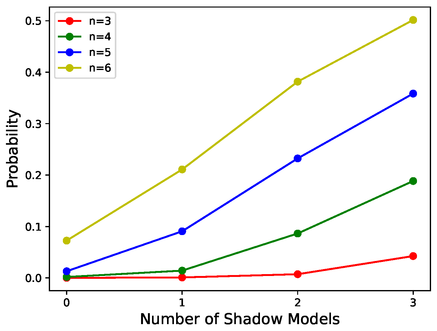
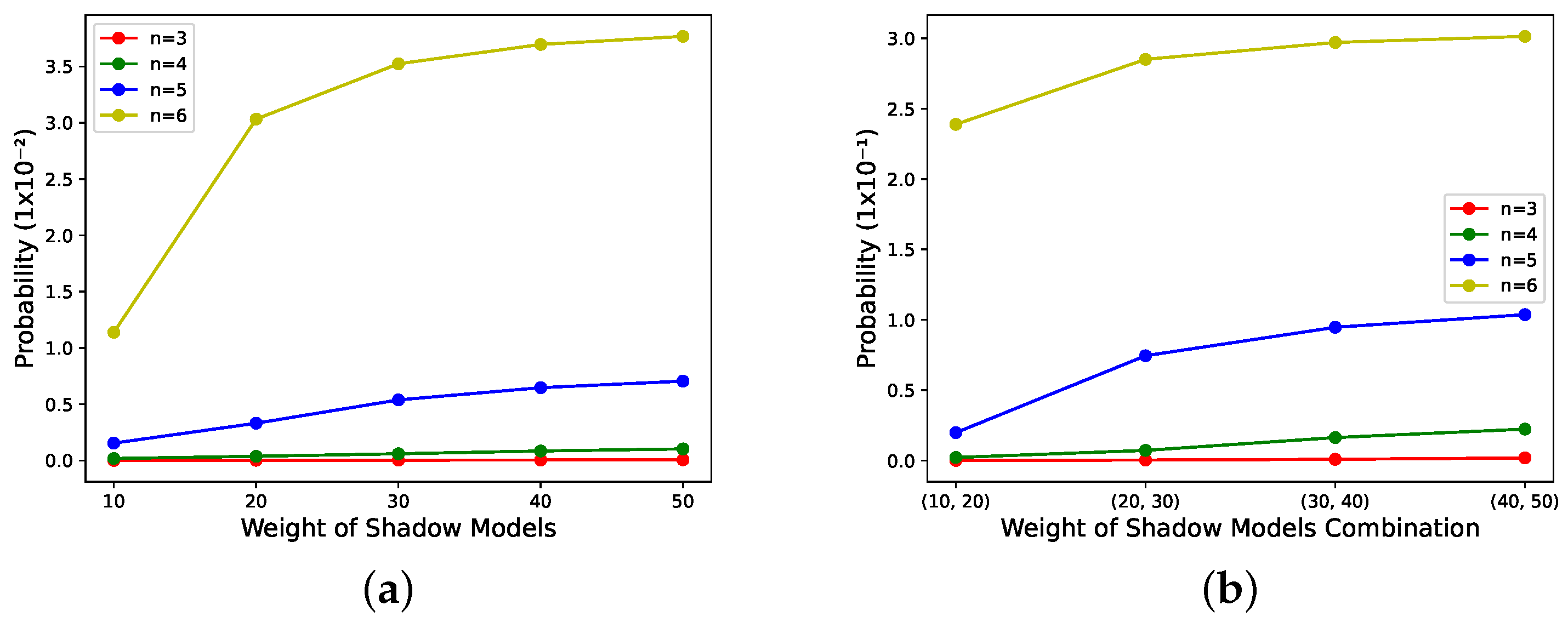
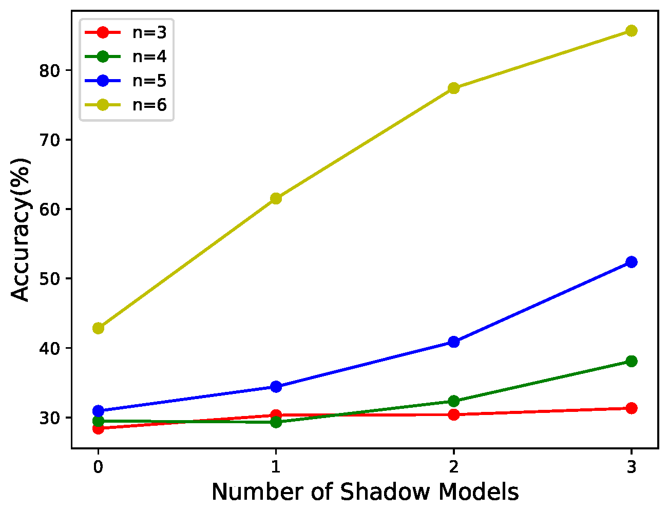
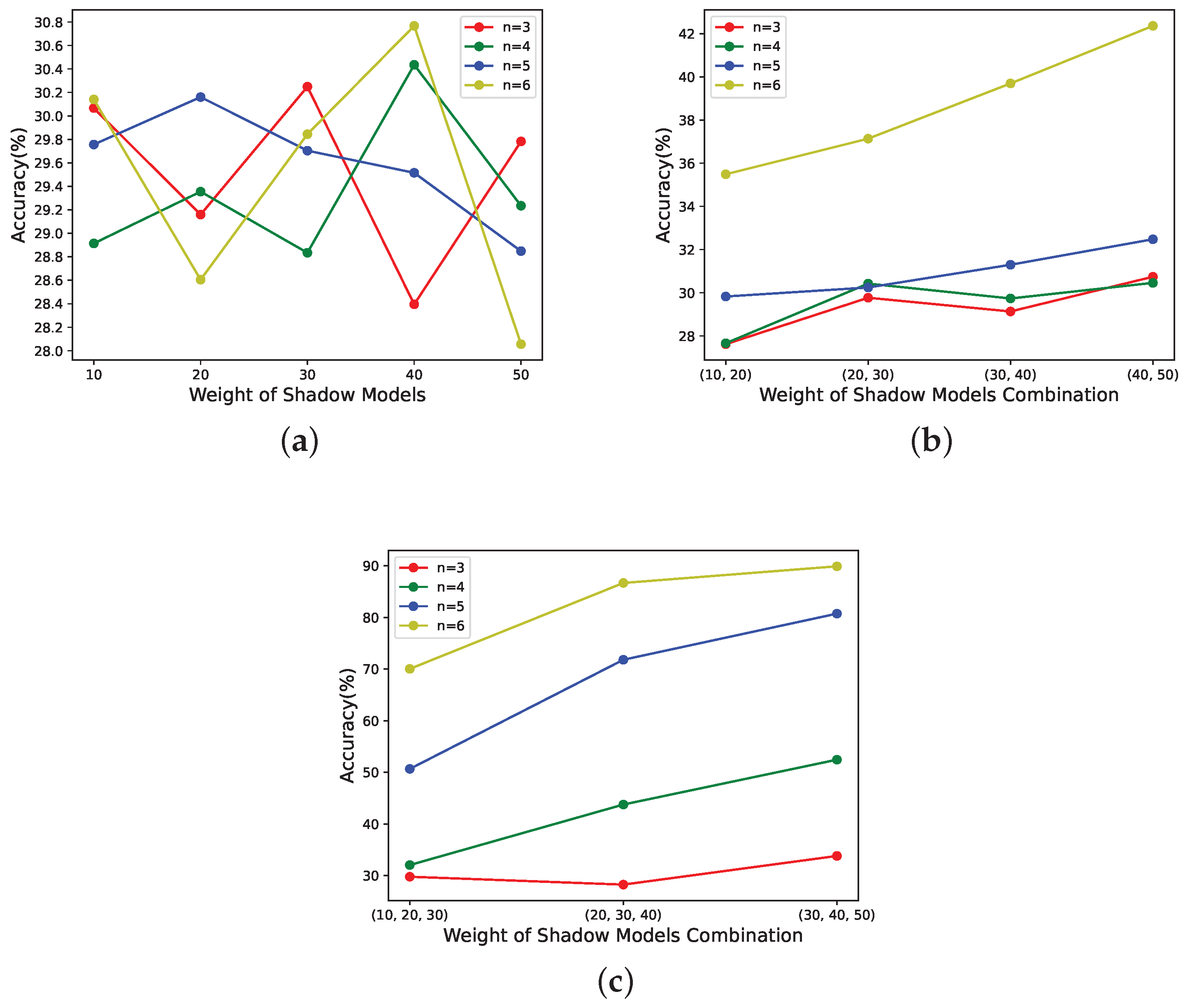
For -threshold NNSS with the weights of {10,10,10,1,1,1,1,1,1,1}, is related to the number of shadow models with weight of 10 in , as shown in Figure 4 when . For -threshold NNSS with the weights of as {10,20,30,40,50,1,1,1,1,1}, is related to shadow models with weights other than 1 in when , as shown in Figure 5.
The above results show that the scheme proposed in this paper is feasible in weight validity. Its weight validity is inferred as follows. The larger the sum of weights of , the higher the performance of the reconstructed model for a determined sharing state. However, either figure’s weight validity is not obvious or almost non-existent when . As the probability of obtaining a valid integer for the secret models with weights of 1 at is minuscule, when the number of shadow models with weights other than 1 in is less than 3, is limited by the probability of obtaining valid integers for shadow models with weights of 1. As n increases, the proportion of candidate shadow models with weights of 1 increases, and its limitation on becomes smaller and smaller. The weight validity is reflected.
4. Experiments and Comparisons
In this section, we will use experiments to demonstrate the progressivity and weight validity of NNSS and analyze the experimental results compared to the theoretical results of the feasibility analyses in the previous section. Since there has not been any research on applying SSS to model sharing, this section will compare the NNSS scheme qualitatively with other model permission-control schemes.
4.1. Experiments and Analyses
This paper validates the proposed scheme using the classification model VGG19 trained on CIFAR-10. The CIFAR-10 dataset consists of 10 categories of 32 × 32 color images, containing a total of 60,000 images, each containing 6000 images. The CIFAR-10 dataset is divided into five training and one test batch, each containing 10,000 images. The test-set batch consists of 1000 images randomly selected from each category, and the training-set batch contains the remaining 50,000 images in a random order. The working environment of the experiments is as follows: windows 11 ver 21H2 22000.675, python 3.8, PyTorch 1.10.0, Cuda 26.21.14.4166, NVIDIA Quadro P5000 (16 G), Intel(R) Xeon(R) CPU E5-2620 v4. The classification accuracy of this model after pre-training is 91.16%. The relevant parameters during the experiments are shown in Table 2.
The reasons for choosing the VGG19 model are as follows. First, according to the study of Tian [16], encrypting the parameters of the VGG model by a few layers can control the model’s performance to a greater extent. Second, VGG19 is a classification model with a greater tolerance for fluctuations in the output results in terms of values than models with complex output results such as the style migration model. Therefore, the NNSS experiments on VGG19 can be effectively conducted.
The scenario we choose in our experiments is the same as the one for which is computed in Section 3.3.1. Considering the random nature of the shadow-model parameters generated and the models selected in the recovery phase, we performed 20 experiments. We averaged them for each -threshold NNSS determined by k, n and model weights.
Specifically, for different determined sharing states, with n in [3, 6] and x in [2, 10] for the -threshold NNSS, the relationship between x and the performance of the reconstructed model is shown in Figure 6, and with k in [2, 6] and x in [1, 10] for the -threshold NNSS, the relationship between x and the performance of the reconstructed model is shown in Figure 7. The correspondence between the subgraph, candidate-shadow-model weights and shadow-model weights is shown in Table 1.
For -threshold NNSS with the weights of as {10,10,10,1,1,1,1,1,1,1}, the performance of the reconstructed model is related to the number of shadow models with a weight of 10 in , as shown in Figure 8 when . For -threshold NNSS with the weights of as {10,20,30,40,50,1,1,1,1,1}, the performance of the reconstructed model is related to the shadow models with weights other than 1 in when , as shown in Figure 9.
From the above experiments, it can be found that:
- According to Figure 6 and Figure 7, it can be seen that the scheme proposed in this paper is progressive. In addition, the progressive effect is consistent with that postulated in the last paragraph, in Section 3.3.1.
- According to Figure 9a, when the number of shadow models with large weights involved in the recovery phase is much smaller than k, the performance of the reconstructed model does not correlate with the weights of the shadow models in the recovery phase. The reason may be that the number of significant parameters recovered is so tiny that it does not offset the performance impact of the randomness of the recovered parameters. The low number of important parameters was described in the last paragraph of Section 3.3.2.
- According to Figure 8 and Figure 9b,c, it can be seen that this scheme has weight validity when the number of shadow models with large weights is involved in the recovery, and the values of n are large. The larger their values are, the stronger the correlation between the performance of the reconstructed model and the weights of the shadow models in the recovery phase.
4.2. Comparison with Other Schemes
No research has been proposed to apply SS to model permission control while existing model permission-control strategies mainly contain digital watermarking and encryption of models. Thus, this subsection compares the NNSS scheme with multiple weights for a progressive recovery scheme with digital watermarking and encryption schemes.
Embedding a digital watermark into a model generally occurs during the model’s training. It can confirm the ownership of the model after piracy occurs [29]. The timing of using an encrypted model is different from that of digital watermarking. It can verify the visitor’s privileges when the model is used. The hierarchical service of the model can be achieved by giving different keys to different users. The NNSS scheme in this paper is one of the encryption schemes that enables permission control of the common training models in the federation. It also enables the progressive recovery of models and control over participants’ weights.
The comparison of the NNSS scheme with other encryption schemes in terms of complexity is shown in Table 3. The number of model parameters being encrypted is h. In the NNSS scheme proposed in this paper, m copies of candidate shadow models need to be generated in the encryption phase, so the space complexity is . As only part of the parameters needs to be encrypted, the time required for the NNSS scheme will be less than the general encryption scheme. However, the number of parameters of the encrypted part is related to h, so the time complexity is still .
Although the advantages of the NNSS scheme proposed are small in terms of complexity, the increase in space complexity is exchanged for more features. Compared with other encryption schemes, the NNSS scheme can achieve hierarchical performance control during the recovery phase without requiring the dealer to provide keys. It is also highly fault-tolerant. Even if a few shadow models are lost, it can allow the reconstructed model to keep a certain performance. If the number of distributed shadow models is greater than t, then a full-performance model can still be recovered when shadow models are lost. The shadow models also have a certain performance, so they are more concealed during the transmission process. At the same time, the sharing phase can be controlled by adjusting the value of n for progressivity.
5. Conclusions
This paper proposes a -threshold NNSS scheme with multiple weights for progressive recovery. It enables progressive recovery and the control of the participants’ weights in the recovery phase. The feasibility of the proposed scheme is verified by calculating the probability of the successful recovery of important parameters and evaluating the performance of the reconstructed model. When the number x of shadow models involved in the recovery phase is greater than k, the larger x is, the better the reconstructed model’s performance. When , the performance of the reconstructed model is comparable to that of the secret model. Compared with other deep-learning permission-control schemes, our scheme has the advantages of high fault tolerance, high concealment, and the ability to control participants’ weights. However, there are still some issues that need to be fixed in future research:
- It is currently only applicable to classification models and may be challenging for applications on models with a high complexity of output results, such as style migration.
- There is a minimum number of participants k in the recovery phase. It will not be possible to calculate any important parameter values for the reconstructed model for fewer than k participants.
Author Contributions
Conceptualization, X.W. and L.Y.; Formal analysis, X.Y. and Y.Y.; Methodology, X.W. and H.S.; Writing—original draft, X.W. All authors have read and agreed to the published version of the manuscript.
Funding
This research is funded by the National Natural Science Foundation of China (Grant Number: 61602491).
Institutional Review Board Statement
Not applicable.
Informed Consent Statement
Not applicable.
Data Availability Statement
Not applicable.
Acknowledgments
The authors would like to thank the editor and the anonymous reviewers for their valuable comment.
Conflicts of Interest
The authors declare no conflict of interest.
References
- Esteva, A.; Chou, K.; Yeung, S.; Naik, N.; Madani, A.; Mottaghi, A.; Liu, Y.; Topol, E.; Dean, J.; Socher, R. Deep learning-enabled medical computer vision. NPJ Digit. Med. 2021, 4, 1–9. [Google Scholar] [CrossRef] [PubMed]
- He, K.; Zhang, X.; Ren, S.; Sun, J. Deep residual learning for image recognition. In Proceedings of the IEEE Conference on Computer Vision and Pattern Recognition, Las Vegas, NV, USA, 27–30 June 2016; pp. 770–778. [Google Scholar]
- Voulodimos, A.; Doulamis, N.; Doulamis, A.; Protopapadakis, E. Deep learning for computer vision: A brief review. Comput. Intell. Neurosci. 2018, 2018, 7068349. [Google Scholar] [CrossRef] [PubMed]
- Rebai, I.; BenAyed, Y.; Mahdi, W.; Lorré, J.P. Improving speech recognition using data augmentation and acoustic model fusion. Procedia Comput. Sci. 2017, 112, 316–322. [Google Scholar] [CrossRef]
- LeCun, Y.; Bottou, L.; Bengio, Y.; Haffner, P. Gradient-based learning applied to document recognition. Proc. IEEE 1998, 86, 2278–2324. [Google Scholar] [CrossRef] [Green Version]
- Sennrich, R.; Haddow, B.; Birch, A. Neural machine translation of rare words with subword units. arXiv 2015, arXiv:1508.07909. [Google Scholar]
- Wu, Y.; Schuster, M.; Chen, Z.; Le, Q.V.; Norouzi, M.; Macherey, W.; Krikun, M.; Cao, Y.; Gao, Q.; Macherey, K.; et al. Google’s neural machine translation system: Bridging the gap between human and machine translation. arXiv 2016, arXiv:1609.08144. [Google Scholar]
- Young, T.; Hazarika, D.; Poria, S.; Cambria, E. Recent trends in deep learning based natural language processing. IEEE Comput. Intell. Mag. 2018, 13, 55–75. [Google Scholar] [CrossRef]
- Karim, M.R.; Beyan, O.; Zappa, A.; Costa, I.G.; Rebholz-Schuhmann, D.; Cochez, M.; Decker, S. Deep learning-based clustering approaches for bioinformatics. Brief. Bioinform. 2021, 22, 393–415. [Google Scholar] [CrossRef] [PubMed] [Green Version]
- Min, S.; Lee, B.; Yoon, S. Deep learning in bioinformatics. Brief. Bioinform. 2017, 18, 851–869. [Google Scholar] [CrossRef] [PubMed] [Green Version]
- Hitaj, D.; Mancini, L.V. Have you stolen my model? Evasion attacks against deep neural network watermarking techniques. arXiv 2018, arXiv:1809.00615. [Google Scholar]
- Zhang, J.; Gu, Z.; Jang, J.; Wu, H.; Stoecklin, M.P.; Huang, H.; Molloy, I. Protecting intellectual property of deep neural networks with watermarking. In Proceedings of the 2018 on Asia Conference on Computer and Communications Security, Incheon, Korea, 4 June 2018; pp. 159–172. [Google Scholar]
- Wang, J.; Wu, H.; Zhang, X.; Yao, Y. Watermarking in deep neural networks via error back-propagation. Electron. Imaging 2020, 2020, 22-1–22-9. [Google Scholar] [CrossRef]
- Rivest, R.L.; Shamir, A.; Adleman, L. A method for obtaining digital signatures and public-key cryptosystems. Commun. ACM 1978, 21, 120–126. [Google Scholar] [CrossRef]
- Verma, A. Encryption and Real Time Decryption for protecting Machine Learning models in Android Applications. arXiv 2021, arXiv:2109.02270. [Google Scholar]
- Tian, J.; Zhou, J.; Duan, J. Probabilistic Selective Encryption of Convolutional Neural Networks for Hierarchical Services. In Proceedings of the IEEE/CVF Conference on Computer Vision and Pattern Recognition, Nashville, TN, USA, 20–25 June 2021; pp. 2205–2214. [Google Scholar]
- Chen, M.; Wu, M. Protect your deep neural networks from piracy. In Proceedings of the 2018 IEEE International Workshop on Information Forensics and Security (WIFS), Hong Kong, China, 11–13 December 2018; pp. 1–7. [Google Scholar]
- Shamir, A. How to share a secret. Commun. ACM 1979, 22, 612–613. [Google Scholar] [CrossRef]
- Blakley, G.R. Safeguarding cryptographic keys. In Proceedings of the Managing Requirements Knowledge, International Workshop on. IEEE Computer Society, New York, NY, USA, 4–7 June 1979; p. 313. [Google Scholar]
- Hou, Y.C.; Quan, Z.Y.; Tsai, C.F. A privilege-based visual secret sharing model. J. Vis. Commun. Image Represent. 2015, 33, 358–367. [Google Scholar] [CrossRef]
- Liu, F.; Yan, X.; Liu, L.; Lu, Y.; Tan, L. Weighted visual secret sharing with multiple decryptions and lossless recovery. Math. Biosci. Eng. 2019, 16, 5750–5764. [Google Scholar] [CrossRef] [PubMed]
- Yu, Y.; Li, L.; Lu, Y.; Yan, X. On the value of order number and power in secret image sharing. Secur. Commun. Netw. 2020, 2020, 6627178. [Google Scholar] [CrossRef]
- Wang, Y.; Chen, J.; Gong, Q.; Yan, X.; Sun, Y. Weighted Polynomial-Based Secret Image Sharing Scheme with Lossless Recovery. Secur. Commun. Netw. 2021, 2021, 5597592. [Google Scholar] [CrossRef]
- Zhang, J.; Chen, D.; Liao, J.; Fang, H.; Zhang, W.; Zhou, W.; Cui, H.; Yu, N. Model watermarking for image processing networks. In Proceedings of the AAAI Conference on Artificial Intelligence, New York, NY, USA, 7–12 February 2020; Volume 34, pp. 12805–12812. [Google Scholar]
- Morcos, A.S.; Barrett, D.G.; Rabinowitz, N.C.; Botvinick, M. On the importance of single directions for generalization. arXiv 2018, arXiv:1803.06959. [Google Scholar]
- Shrikumar, A.; Greenside, P.; Kundaje, A. Learning important features through propagating activation differences. In Proceedings of the International Conference on Machine Learning, Sydney, Australia, 6–11 August 2017; pp. 3145–3153. [Google Scholar]
- Yu, R.; Li, A.; Chen, C.F.; Lai, J.H.; Morariu, V.I.; Han, X.; Gao, M.; Lin, C.Y.; Davis, L.S. Nisp: Pruning networks using neuron importance score propagation. In Proceedings of the IEEE Conference on Computer Vision and Pattern Recognition, Salt Lake City, UT, USA, 18–23 June 2018; pp. 9194–9203. [Google Scholar]
- Papernot, N.; McDaniel, P.; Sinha, A.; Wellman, M.P. Sok: Security and privacy in machine learning. In Proceedings of the 2018 IEEE European Symposium on Security and Privacy (EuroS&P), London, UK, 24–26 April 2018; pp. 399–414. [Google Scholar]
- Wang, X.; Lu, Y.; Yan, X.; Yu, L. Wet Paper Coding-Based Deep Neural Network Watermarking. Sensors 2022, 22, 3489. [Google Scholar] [CrossRef] [PubMed]
Figure 1.
Workflow diagram of the NNSS scheme proposed in this paper.

Figure 2.
When k is constant, the relationship between x and for different determined sharing states. (a) All candidate shadow models’ weights and shadow models’ weights are 1. (b) 3 of candidate shadow models’ weights are 10, and the rest are 1. 3 of shadow models’ weights are 10, and the rest are 1. (c) 3 of candidate shadow models’ weights are 1, and the rest are 10. 3 of shadow models’ weights are 1, and the rest are 10.

Figure 3.
When n is constant, the relationship between x and for different determined sharing states. (a) All candidate shadow models’ weights and shadow models’ weights are 1. (b) 3 of candidate shadow models’ weights are 10, and the rest are 1. 3 of shadow models’ weights are 10, and the rest are 1. (c) 3 of candidate shadow models’ weights are 1, and the rest are 10. 3 of shadow models’ weights are 1, and the rest are 10.

Figure 4.
The relationship between and number of shadow models with weight of 10 for different determined sharing states.
Figure 4.
The relationship between and number of shadow models with weight of 10 for different determined sharing states.

Figure 5.
The relationship between and weight of shadow models with the weights other than 1 for different determined sharing states. (a) The number of shadow models with weights other than 1 in is 1. (b) The number of shadow models with weights other than 1 in is 2.
Figure 5.
The relationship between and weight of shadow models with the weights other than 1 for different determined sharing states. (a) The number of shadow models with weights other than 1 in is 1. (b) The number of shadow models with weights other than 1 in is 2.

Figure 6.
When k is constant, the relationship between x and the performance of reconstructed model for different determined sharing states. (a) All candidate shadow models’ weights and shadow models’ weights are 1. (b) 3 of candidate shadow models’ weights are 10, and the rest are 1. 3 of shadow models’ weights are 10, and the rest are 1. (c) 3 of candidate shadow models’ weights are 1, and the rest are 10. 3 of shadow models’ weights are 1, and the rest are 10.

Figure 7.
When n is constant, the relationship between x and the performance of reconstructed model for different determined sharing states. (a) All candidate shadow models’ weights and shadow models’ weights are 1. (b) 3 of candidate shadow models’ weights are 10, and the rest are 1. 3 of shadow models’ weights are 10, and the rest are 1. (c) 3 of candidate shadow models’ weights are 1, and the rest are 10. 3 of shadow models’ weights are 1, and the rest are 10.

Figure 8.
The relationship between the performance of reconstructed model and number of shadow models with weight of 10 for different determined sharing states.
Figure 8.
The relationship between the performance of reconstructed model and number of shadow models with weight of 10 for different determined sharing states.

Figure 9.
The relationship between the performance of reconstructed model and weight of shadow models with the weights other than 1 for different determined sharing states. (a) The number of shadow models with weights other than 1 in is 1. (b) The number of shadow models with weights other than 1 in is 2. (c) The number of shadow models with weights other than 1 in is 3.


Table 1.
The correspondence between the subgraph and the determined sharing state.
| Subfigure Number | Candidate Shadow Models’ Weight | Shadow Models’ Weight |
|---|---|---|
| a | all of them are 1 | all of them are 1 |
| b | 3 of them are 10, the rest are 1 | 3 of them are 10, the rest are 1 |
| c | 3 of them are 1, the rest are 10 | 3 of them are 1, the rest are 10 |
Table 2.
The relevant parameters during the experiments.
| Parameter | Value |
|---|---|
| The number of layers where important parameters are located in VGG19 | 1, 2, 3 |
| Ratio of important parameters per layer | 2% |
| Finite field prime P | 40,009 |
| Deviation | 1.5 |
| Precision R | 2 |
Table 3.
The comparison of the NNSS scheme with other encryption schemes.
| Complexity | The NNSS Scheme | General Encryption Scheme | Encryption Scheme with Selection Strategy |
|---|---|---|---|
| Time Complexity | |||
| Space Complexity |
Publisher’s Note: MDPI stays neutral with regard to jurisdictional claims in published maps and institutional affiliations. |
© 2022 by the authors. Licensee MDPI, Basel, Switzerland. This article is an open access article distributed under the terms and conditions of the Creative Commons Attribution (CC BY) license (https://creativecommons.org/licenses/by/4.0/).
Share and Cite
MDPI and ACS Style
Wang, X.; Shan, H.; Yan, X.; Yu, L.; Yu, Y. A Neural Network Model Secret-Sharing Scheme with Multiple Weights for Progressive Recovery. Mathematics 2022, 10, 2231. https://doi.org/10.3390/math10132231
AMA Style
Wang X, Shan H, Yan X, Yu L, Yu Y. A Neural Network Model Secret-Sharing Scheme with Multiple Weights for Progressive Recovery. Mathematics. 2022; 10(13):2231. https://doi.org/10.3390/math10132231
Chicago/Turabian StyleWang, Xianhui, Hong Shan, Xuehu Yan, Long Yu, and Yongqiang Yu. 2022. "A Neural Network Model Secret-Sharing Scheme with Multiple Weights for Progressive Recovery" Mathematics 10, no. 13: 2231. https://doi.org/10.3390/math10132231
Note that from the first issue of 2016, this journal uses article numbers instead of page numbers. See further details here.