One- and Two-Dimensional Analytical Solutions of Thermal Stress for Bimodular Functionally Graded Beams under Arbitrary Temperature Rise Modes

Abstract

In this study, we analytically solved the thermal stress problem of a bimodular functionally graded bending beam under arbitrary temperature rise modes. First, based on the strain suppression method in a one-dimensional case, we obtained the thermal stress of a bimodular functionally graded beam subjected to bending moment under arbitrary temperature rise modes. Using the stress function method based on compatibility conditions, we also derived two-dimensional thermoelasticity solutions for the same problem under pure bending and lateral-force bending, respectively. During the solving, the number of unknown integration constants is doubled due to the introduction of bimodular effect; thus, the determination for these constants depends not only on the boundary conditions, but also on the continuity conditions at the neutral layer. The comparisons indicate that the one- and two-dimensional thermal stress solutions are consistent in essence, with a slight difference in the axial stress, which exactly reflects the distinctions of one- and two-dimensional problems. In addition, the temperature rise modes in this study are not explicitly indicated, which further expands the applicability of the solutions obtained. The originality of this work is that the one- and two-dimensional thermal stress solutions for bimodular functionally graded beams are derived for the first time. The results obtained in this study may serve as a theoretical reference for the analysis and design of beam-like structures with obvious bimodular functionally graded properties in a thermal environment.

1. Introduction

In the classical theory of elasticity by Timoshenko and Goodier [1], the theoretical analysis for thermal stress began with the boundary force problem, that is, a rectangular section bar with uniform thickness is subjected to a temperature change. Basically, there are two common methods to analyze the thermal stress. One is the strain suppression method used in a one-dimensional case and the other is the two-dimensional thermoelasticity method, each having its own characteristics. The material considered in the thermal stress problem is homogeneous, elastic and isotropic. However, with the development of material technology, many new materials with certain functions are constantly emerging, some of which present the diversity of materials; this makes the analysis of classical materials more difficult [2,3,4,5,6,7]. For example, to eliminate the interface effect and relieve heat stress, functionally graded materials (FGMs) were created. Many studies indicate that most materials will exhibit different tensile and compressive strains when they are subjected to tensile and compressive stresses, that is, the materials have a bimodular effect. Obviously, the introduction of the new material properties leads, to some extent, to routine analysis becoming inadequate, especially when an appropriate analytical method is necessary. Thus, our work will focus on the corresponding analytical methods for this problem. The relevant work is reviewed from the following three aspects: the existing work on beams with the FGM characteristic or bimodular effect, the corresponding analytical methods, and our innovative work conducted in this study.

To avoid thermal stress and eliminate the interface effect, the idea of functionally graded materials was proposed by Japanese scientists. This kind of material possesses properties that vary gradually with location within the material. There are many mathematical approximations to model the variation of properties in FGMs. One of them is exponential variation, where the elastic constants vary in the light of the form of exponential function. Due to the convenience in mathematical treatment, many researchers adopted exponential function in solving elasticity problems. An elasticity solution for a functionally graded beam subjected to transverse loads was obtained by Sankar [8], in which the Young’s modulus is assumed to vary exponentially along the thickness direction. Sankar and co-workers also studied the relative issues of functionally graded beams including a sandwich beam with a functionally graded core [9], thermal stresses [10], and a combined Fourier series–Galerkin method [11]. Without specifying the graded variations of the material properties, Zhong and co-workers obtained a general solution of a functionally graded beam using the stress function method [12] and displacement function method [13], respectively, and also presented the exact solutions for elastoplastic stress distribution in functionally graded curved beams under pure bending [14]. Giunta et al. [15] proposed several axiomatic refined theories for the linear static analysis of beams whose material properties are graded along one or two directions. Menaa et al. [16] used the energy equivalence principle to derive a general expression for the static shear correction factors of functionally graded beams. There is a lot of research on FGM beams, which is not reviewed here.

Compared with FGM, bimodular material [17] seems to have entered the field of view of scholars later. Many studies have indicated that most materials [18,19], including concrete, ceramics, graphite, rubber and biomedical materials, exhibit different tensile and compressive strains under the same stress applied in tension or compression. These materials are known as bimodular materials. Overall, there are two basic material models widely used in theoretical analysis within the engineering profession. One is the positive-negative signs criterion in the longitudinal fiber strains proposed by Bert [20]. This model is mainly applied to orthotropic materials and, therefore, is widely used for studies on laminated composites [21,22,23,24]. Another model is the positive-negative signs criterion of principal stress presented by Ambartsumyan [25], which is mainly applicable to isotropic materials. In the structural analysis for beams, plates and shells, the stress state along a certain principal direction is a key issue, because it is this factor that determines whether the point is in tension or in compression. Ambartsumyan [25] adopted two straight lines whose tangents at the origin are discontinuous to linearize the bimodular materials model, as shown in Figure 1. Due to the fact that this bimodular theory defines its constitutive model on principal stress directions, where the principal stress is generally obtained as a final result, but not as a known condition before solving, the description of the stress state of a point becomes inevitably difficult. At the same time, this model lacks the ability to describe the experimental results of elastic coefficients in the state of complex stress. Analytical solutions are available in a few cases, generally in simple cases on beams and plates [26,27,28,29]. In some complex problems, it is necessary to resort to the finite element method (FEM) based on an iterative technique [30,31,32,33,34]. Thus, the analytical study of bimodular problems is somewhat challenging.

By combining the functionally graded property and bimodular effect of materials, some scholars began to study bimodular FGM beam problems in the last ten years. These studies mainly include the bimodular FGM straight beam [35], bimodular FGM curved beam [36], or the bimodular FGM piezoelectric beam [37,38]. However, among these studies on bimodular FGM beams, the relevant thermal stress problem has not been found. This appears to be lacking because an important purpose of creating FGMs is to relieve the thermal stress generated under high-temperature conditions.

From the viewpoint of analytical methods, the problem of thermal stress must be solved using the theory of thermoelasticity. In thermoelasticity [39], the influence of the temperature field in the governing equations is presented through constitutive law. Linear thermoelasticity is established on the linear supplement of thermal strains to mechanical strains. Generally, there are two basic methods used in problems of thermoelasticity. One is the displacement method, in which problems of thermoelasticity are solved by finding solutions to Lamé displacement equations when a body is acted upon by arbitrary mass forces. Thus, many basic thermoelasticity problems are considered within the classical theory of elasticity. This is the known body force analogy method, which may date back to Duhamel, who made great contributions to this field in history. Of course, the problems of thermoelasticity are also solved by another basic method, that is, the stress method based on compatibility relations, in which the stress, but not the displacement, is selected as an unknown basic variable.

More recently, based on the classical body force analogy method, Wen et al. [40] obtained a two-dimensional thermoelasticity solution of a bimodular beam under the combined action of thermal and mechanical loads. Also based on this method, Guo et al. [41] theoretically analyzed a metal bar with bimodular effect only under the thermal loads, in which three temperature rise modes including linear, square and cubic variations along the thickness direction of the beam are considered. In previous studies [40,41], these solutions to the plane thermal stress problem were derived by selecting displacement as a basic variable, since the introduction of the bimodular effect does not change the basic form of the Lamé equation. Therefore, the classical Duhamel theorem concerning the body force analogy may be adopted to transform the thermal plane stress problem into a classical plane stress problem. However, if we introduce not only the bimodular effect of the materials, but also the functionally graded property, the resulting Lamé equation will change significantly in form, thus making the application of the Duhamel theorem impossible. In this case, adopting the stress method based on compatibility conditions is the only option.

Using the appropriate analytical methods, this study is dedicated to obtaining one- and two-dimensional analytical solutions to the thermal stress of a bimodular FGM beam under arbitrary temperature rise modes. Parametric study is not the main purpose of this study, although the obtainment of analytical solutions is very helpful for parametric study. The novelties and main contributions of this work are to introduce, for the first time, the bimodular functionally graded property of materials into the thermal stress problem of the beams. The resulting problems of deep beams and shallow beams in a thermal environment are also solved in a one-dimensional case and two-dimensional case, respectively. The paper is organized as follows. First, in Section 2, the strain suppression method is used for determining the one-dimensional solution of a bimodular FGM beams. Adopting the stress function method of thermoelasticity, in Section 3, the two-dimensional solutions for the same problem are obtained under pure bending and lateral-force bending. The comparison of the one- and two-dimensional solutions and the comparison under pure bending and lateral-force bending of the two-dimensional problems, as well as the regression and validation of the solutions, are given in Section 4 in detail. The numerical results and the corresponding discussions are given in Section 5. Section 6 presents the concluding remarks.

2. Strain Suppression Method in One-Dimensional Case

In the one-dimensional case, we use the strain suppression method to derive the thermal stress solution of a bimodular functionally graded beam under thermal and mechanical loads. The basic assumptions in the next derivation are as follows. (i) The initial neutral axis only depends on the bending moment, not on the thermal loads—that is to say, the thermal load is applied after the action of the bending moment. (ii) Like common shallow beams, the bending is limited in plane small-deflection bending without torsion, the cross-section of the beam keeps plane after bending, and there is no extrusion between the longitudinal fibers in the beam. (iii) The material of the beam is considered to be linear elastic, but at the same time, the bimodular effect and functional-grade characteristic are incorporated. (iv) The temperature only varies with the height direction of the beam.

A bimodular FGM beam with a rectangular section dimension h × b is subjected to the combined action of bending moment M at its two ends and the temperature rise T(z), as shown in Figure 2, in which the x-axis is located on the neutral axis caused by the action of the bending moment alone, the y-axis is along the thickness direction and the z-axis along the height direction; thus, the o-xyz coordinate system is established. Note that due to the introduction of the bimodular functionally graded characteristic of the materials, the tensile and compressive section height of the beam is now h₁ and h₂, respectively, and the modulus of elasticity in the tensile and compressive zone is E⁺(z) and E⁻(z), respectively, while the Poisson’s ratio remains the same. In addition, the line expansion coefficient α is regarded as the function of z, but there is no difference in tension and compression, that is, α = α(z).

For the convenience of mathematical treatment, we introduce exponential functions to express E⁺(z), E⁻(z) and α(z), such that

$$E^{+}(z)=E_0{e}^{a_{1}z/h}, E^{-}(z)=E_0{e}^{a_{2}z/h}, \alpha (z)={\alpha }_0{e}^{cz/h},$$

(1)

where a₁ and a₂ are two dimensionless grade parameters, and they satisfy E⁺(z) = E⁻(z) = E₀ when a₁ = a₂ = 0 or when z = 0, and E₀ is the elastic modulus of materials at the neutral axis. Similarly, c is also a grade parameter, and α(z) = α₀ when c = 0 or when z = 0.

According to the strain suppression method, the total strain in the beam consists of three parts; they are the compressive suppression strain ε_s, the axial strain ε_a and the bending strain ε_b, which may be written as [1]

$${\epsilon }_x={\epsilon }_s+{\epsilon }_a+{\epsilon }_b,$$

(2)

where the three strains may be expressed as, by definition,

$${\epsilon }_s=-\alpha (z)T(z), {\epsilon }_a=\frac{{\displaystyle \int E(z)\alpha (z)T(z)}dz}{{\displaystyle \int E(z)}dz}, {\epsilon }_b=\frac{{\displaystyle \int E(z)\alpha (z)T(z)z}dz}{{\displaystyle \int E(z)z^2}dz}z.$$

(3)

Thus, the total strain is

$${\epsilon }_x=\left[-\alpha (z)T(z)+\frac{{\displaystyle \int E(z)\alpha (z)T(z)}dz}{{\displaystyle \int E(z)}dz}+\frac{{\displaystyle \int E(z)\alpha (z)T(z)z}dz}{{\displaystyle \int E(z)z^2}dz}z\right].$$

(4)

According to Hooke’s Law, σ_x = E(z)ε_x; for a bimodular problem in the tensile and compressive zone, that is, 0 ≤ z ≤ h₁ and −h₂ ≤ z ≤ 0, we have the stress

$$\{\begin{array}{l}{\sigma }_x^{+}=E^{+}(z){\epsilon }_x, \mathrm{at} 0\le z\le h_1\\ {\sigma }_x^{-}=E^{-}(z){\epsilon }_x, \mathrm{at} -h_2\le z\le 0 \end{array},$$

(5)

Substituting Equation (1) into Equations (4) and (5), and also noting that the integration operation should be carried out according to the tensile areas and compressive areas, we have the stress

$$\{\begin{array}{l}{\sigma }_x^{+}=E_0{e}^{a_{1}z/h}\left[-{\alpha }_0{e}^{cz/h}T(z)+\frac{{\alpha }_0(T_0^{+}+T_0^{-})}{A_0^{+}+A_0^{-}}+\frac{{\alpha }_0(T_1^{+}+T_1^{-})}{A_2^{+}+A_2^{-}}z\right] \mathrm{at} 0\le z\le h_1\\ {\sigma }_x^{-}=E_0{e}^{a_{2}z/h}\left[-{\alpha }_0{e}^{cz/h}T(z)+\frac{{\alpha }_0(T_0^{+}+T_0^{-})}{A_0^{+}+A_0^{-}}+\frac{{\alpha }_0(T_1^{+}+T_1^{-})}{A_2^{+}+A_2^{-}}z\right] \mathrm{at} -h_2\le z\le 0\end{array},$$

(6)

where

$$\{\begin{array}{l}{A}_0{}^{+}={\displaystyle {\int }_0^{h_1}{e}^{a_{1}z/h}}dz, A_0{}^{-}={\displaystyle {\int }_{-h_2}^0{e}^{a_{2}z/h}}dz\\ A_1{}^{+}={\displaystyle {\int }_0^{h_1}{e}^{a_{1}z/h}z}dz, A_1{}^{-}={\displaystyle {\int }_{-h_2}^0{e}^{a_{2}z/h}z}dz\\ A_2{}^{+}={\displaystyle {\int }_0^{h_1}{e}^{a_{1}z/h}{z}^2}dz, A_2{}^{-}={\displaystyle {\int }_{-h_2}^0{e}^{a_{2}z/h}{z}^2}dz\\ T_0^{+}={\displaystyle {\int }_0^{h_1}{e}^{\left(a_1+c\right)z/h}Tdz}, T_0^{-}={\displaystyle {\int }_{-h_2}^0{e}^{\left(a_2+c\right)z/h}Tdz}\\ T_1^{+}={\displaystyle {\int }_0^{h_1}{e}^{\left(a_1+c\right)z/h}Tzdz}, T_1^{-}={\displaystyle {\int }_{-h_2}^0{e}^{\left(a_2+c\right)z/h}Tzdz}\end{array},$$

(7)

and the pre-introduction of A₁⁺ and A₁⁻ is also for the convenience of the next derivation.

Following our above assumption, the external bending moment M is applied and at the same time, no any external axial force N is applied here, as shown in Figure 2. According to our previous study [35], we have

$$\{\begin{array}{l}N={\displaystyle {\int }_0^{h_1}{E}_0{e}^{a_{1}z/h}\frac{z}{\rho }}bdz+{\displaystyle {\int }_{-h_2}^0{E}_0{e}^{a_{2}z/h}\frac{z}{\rho }b}dz=0\\ M={\displaystyle {\int }_0^{h_1}{E}_0{e}^{a_{1}z/h}\frac{z^2}{\rho }b}dz+{\displaystyle {\int }_{-h_2}^0{E}_0{e}^{a_{2}z/h}\frac{z^2}{\rho }}bdz\end{array},$$

(8)

this gives

$$A_1{}^{+}+A_1{}^{-}=0, \frac{1}{\rho }=\frac{M}{D^{*}}, D^{*}=E_{0}b(A_2{}^{+}+A_2{}^{-}),$$

(9)

in which D* is the bending stiffness of a bimodular beam, and the relation A₁⁺+ A₁⁻ = 0 is used for the determination of the unknown neutral axis. Now, we need to add the effect of the bending moment into Equation (6); thus, we have

$$\{\begin{array}{l}{\sigma }_x^{+}=E_0{e}^{a_{1}z/h}\left[-{\alpha }_0{e}^{cz/h}T(z)+\frac{{\alpha }_0(T_0^{+}+T_0^{-})}{A_0^{+}+A_0^{-}}+\frac{M/E_{0}b+{\alpha }_0(T_1^{+}+T_1^{-})}{A_2^{+}+A_2^{-}}z\right] \mathrm{at} 0\le z\le h_1\\ {\sigma }_x^{-}=E_0{e}^{a_{2}z/h}\left[-{\alpha }_0{e}^{cz/h}T(z)+\frac{{\alpha }_0(T_0^{+}+T_0^{-})}{A_0^{+}+A_0^{-}}+\frac{M/E_{0}b+{\alpha }_0(T_1^{+}+T_1^{-})}{A_2^{+}+A_2^{-}}z\right] \mathrm{at} -h_2\le z\le 0\end{array}.$$

(10)

Thus, we obtain the one-dimensional thermal stress solution of a bimodular FGM beam under bending moment and thermal load.

3. Two-Dimensional Thermoelasticity Solution

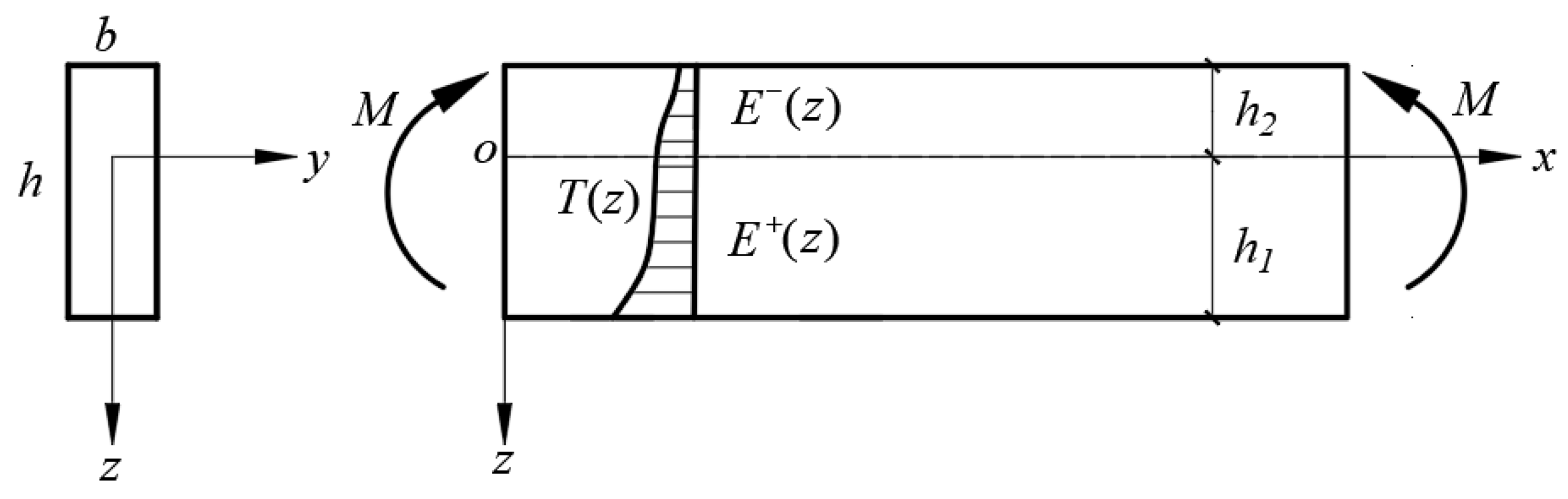
For an effective comparison, we begin with the pure bending case, followed by the lateral-force bending case.

3.1. Pure Bending

Let us first analyze a bimodular FGM cantilever beam under bending moment and thermal load, which is the same as Figure 2, with the exception that the right end of the beam is fixed and the left end is free. The length of the beam is l, as shown in Figure 3, and the definitions for other physical quantities are the same as those in Figure 2.

This problem may be considered a typical plane stress problem concerning thermal effect. If we let σ_x, σ_z and τ_xz be the stress components of a plane stress problem, we have the equation of equilibrium [1], by ignoring the body forces,

$$\frac{\partial {\sigma }_x}{\partial x}+\frac{\partial {\tau }_{xz}}{\partial z}=0, \frac{\partial {\sigma }_z}{\partial z}+\frac{\partial {\tau }_{xz}}{\partial x}=0.$$

(11)

If we let ε_x, ε_z and γ_xz be the strain components of a plane stress problem, and u and w be the displacement components along x and z direction, respectively, we may have the geometrical relation [1]

$${\epsilon }_x=\frac{\partial u}{\partial x}, {\epsilon }_z=\frac{\partial w}{\partial z}, {\gamma }_{xz}=\frac{\partial w}{\partial x}+\frac{\partial u}{\partial z}.$$

(12)

We may also derive the compatibility equation, as follows:

$$\frac{{\partial }^2{\epsilon }_x}{\partial z^2}+\frac{{\partial }^2{\epsilon }_z}{\partial x^2}=\frac{{\partial }^2{\gamma }_{xz}}{\partial x\partial z}.$$

(13)

The basic physical equation in the two-dimensional plane stress problem will give

$$\{\begin{array}{l}{\epsilon }_x=\frac{1}{E^{+/-}(z)}({\sigma }_x-\mu {\sigma }_z)+\alpha (z)T\\ {\epsilon }_z=\frac{1}{E^{+/-}(z)}({\sigma }_z-\mu {\sigma }_x)+\alpha (z)T\\ {\gamma }_{xz}=\frac{2(1+\mu )}{E^{+/-}(z)}{\tau }_{xz}\end{array}.$$

(14)

where T = T(z). If we also introduce the same exponential function to express E⁺(z), E⁻(z) and α(z), as shown in Equation (1), then the physical equation for a bimodular FGM may be changed to

$$\{\begin{array}{l}{\epsilon }_x=\frac{1}{E_0{e}^{a_{i}z/h}}({\sigma }_x-\mu {\sigma }_z)+{\alpha }_0{e}^{cz/h}T\\ {\epsilon }_z=\frac{1}{E_0{e}^{a_{i}z/h}}({\sigma }_z-\mu {\sigma }_x)+{\alpha }_0{e}^{cz/h}T\\ {\gamma }_{xz}=\frac{2(1+\mu )}{E_0{e}^{a_{i}z/h}}{\tau }_{xz}\end{array},$$

(15)

where i = 1,2 (1 for tension and 2 for compression), and the Poisson’s ratio is kept constant.

Let us introduce the stress function ϕ^+/−(x,z) to solve this problem, in which the symbol ‘+” is for tension and ‘−’ for compression. To satisfy the equilibrium Equation (11), we have [1]

$${\sigma }_x^{+/-}=\frac{{\partial }^2{\phi }^{+/-}(x, z)}{\partial z^2}, {\sigma }_z^{+/-}=\frac{{\partial }^2{\phi }^{+/-}(x, z)}{\partial x^2}, {\tau }_{xz}^{+/-}=-\frac{{\partial }^2{\phi }^{+/-}(x, z)}{\partial x\partial z}.$$

(16)

Considering that the load type is pure bending and the temperature change T only changes with z, we may suppose the ϕ^+/−(x,z) as

$${\phi }^{+/-}(x, z)=f_1{}^{+/-}(z),$$

(17)

where f ₁^+/−(z) is an unknown function of z. Substituting it into Equation (16) gives

$${\sigma }_x^{+/-}=\frac{d^2{f}_1^{+/-}(z)}{d{z}^2}, {\sigma }_z^{+/-}=0, {\tau }_{xz}^{+/-}=0,$$

(18)

thus, Equation (15) may be further written as

$$\{\begin{array}{l}{\epsilon }_x=\frac{1}{E_0{e}^{a_{i}z/h}}\frac{d^2{f}_1^{+/-}(z)}{\mathrm{d}{z}^2}+{\alpha }_0{e}^{cz/h}T\\ {\epsilon }_z=-\frac{\mu }{E_0{e}^{a_{i}z/h}}\frac{d^2{f}_1^{+/-}(z)}{\mathrm{d}{z}^2}+{\alpha }_0{e}^{cz/h}T\\ {\gamma }_{xz}=0\end{array}.$$

(19)

Substituting it into Equation (13), we have

$$\frac{d^2}{d{z}^2}\left[\frac{1}{E_0{e}^{a_{i}z/h}}\frac{d^2{f}_1^{+/-}(z)}{d{z}^2}+{\alpha }_0{e}^{cz/h}T\right]=0.$$

(20)

Integrating the above equation with respect z continuously, also noting T = T(z), we have

$$\frac{d^2{f}_1^{+/-}(z)}{d{z}^2}=\left(C_1^{+/-}z+C_2^{+/-}-{\alpha }_0{e}^{cz/h}T\right)E_0{e}^{a_{i}z/h},$$

(21)

$$\frac{d{f}_1^{+/-}(z)}{dz}=\left(z-\frac{h}{a_i}\right)\frac{C_1^{+/-}h{E}_0{e}^{a_{i}z/h}}{a_i}+\frac{C_2^{+/-}h{E}_0{e}^{a_{i}z/h}}{a_i}-{\displaystyle \int E_0{\alpha }_0{e}^{\left(a_i+c\right)z/h}Tdz}+C_3^{+/-},$$

(22)

$$f_1^{+/-}(z)=\left(z-\frac{2h}{a_i}\right)\frac{C_1^{+/-}{h}^2{E}_0{e}^{a_{i}z/h}}{a_i^2}+\frac{C_2^{+/-}{h}^2{E}_0{e}^{a_{i}z/h}}{a_i^2}-{\displaystyle \int \left({\displaystyle \int E_0{\alpha }_0{e}^{\left(a_i+c\right)z/h}Tdz}\right)}dz+C_3^{+/-}z+C_4^{+/-},$$

(23)

in which C₁^+/−, C₂^+/−, C₃^+/− and C₄^+/− are unknown integration constants. Note that C₃^+/− and C₄^+/− may be ignored in the stress function ϕ^+/−(x,z). Thus, we have

$$\begin{array}{cc}\hfill {\phi }^{+/-}(x, z)& =f_1^{+/-}(z)\hfill \\ & =\left(z-\frac{2h}{a_i}\right)\frac{C_1^{+/-}{h}^2{E}_0{e}^{a_{i}z/h}}{a_i^2}+\frac{C_2^{+/-}{h}^2{E}_0{e}^{a_{i}z/h}}{a_i^2}-E_0{\alpha }_0{\displaystyle \int {\displaystyle \int e^{\left(a_i+c\right)z/h}Tdz}}dz\hfill \end{array}.$$

(24)

Via Equations (18) and (21), we have the following stress formulas containing C₁^+/− and C₂^+/−:

$${\sigma }_x^{+/-}=\frac{d^2{f}_1^{+/-}(z)}{d{z}^2}=\left(C_1^{+/-}z+C_2^{+/-}-{\alpha }_0{e}^{cz/h}T\right)E_0{e}^{a_{i}z/h}, {\sigma }_z^{+/-}={\tau }_{zx}^{+/-}=0.$$

(25)

Next, the boundary conditions on the four sides of the beam and continuity conditions on the neutral layer (z = 0) will be used for the determination of C₁^+/− and C₂^+/−.

First, at z = 0, the continuity conditions will give [35]

$${\sigma }_x^{+}={\sigma }_x^{-}, \mathrm{at} z=0.$$

(26)

Applying it to σ_x^+/− in Equation (25), we need to satisfy

$${\sigma }_x^{+}=(C_2^{+}-{\alpha }_{0}T)E_0={\sigma }_x^{-}=(C_2^{-}-{\alpha }_{0}T)E_0.$$

(27)

Obviously,

$$C_2^{+}=C_2^{-}.$$

(28)

In addition, according to the definition for the neutral axis of a bimodular problem, we may have the following strain relation on the neutral axis:

$${\epsilon }_x^{+}={\epsilon }_x^{-}=0, \mathrm{at} z=0.$$

(29)

Combining the first one of Equations (19) and (21), at z = 0, we have,

$$\{\begin{array}{l}{\epsilon }_x^{+}=\frac{1}{E_0}(C_2^{+}-{\alpha }_{0}T)E_0+{\alpha }_{0}T\\ {\epsilon }_x^{-}=\frac{1}{E_0}(C_2^{-}-{\alpha }_{0}T)E_0+{\alpha }_{0}T\end{array}.$$

(30)

According to Equations (29) and (30), we obtain

$$C_2^{+}=C_2^{-}=0.$$

(31)

Now, let us consider the boundary conditions on the four sides. First, on the two main sides, we have

$$\{\begin{array}{l}{\sigma }_z^{+}=0, {\tau }_{xz}^{+}=0, \mathrm{at} z=h_1\\ {\sigma }_z^{-}=0, {\tau }_{xz}^{-}=0, \mathrm{at} z=-h_2\end{array}.$$

(32)

Obviously, they are satisfied naturally and cannot be used for the determination of C₁^+/−. Due to l >> h, at x = 0, we may apply the Saint-Venant principle to obtain three integration equations; this gives

$$\{\begin{array}{l}{\displaystyle {\int }_{-h_2}^0{\sigma }_x^{-}}dz+{\displaystyle {\int }_0^{h_1}{\sigma }_x^{+}}dz=0\hfill \\ {\displaystyle {\int }_{-h_2}^0{\sigma }_x^{-}}zdz+{\displaystyle {\int }_0^{h_1}{\sigma }_x^{+}}zdz=\frac{M}{b}\hfill \\ {\displaystyle {\int }_{-h_2}^0{\tau }_{xz}^{-}}dz+{\displaystyle {\int }_0^{h_1}{\tau }_{xz}^{+}}dz=0\hfill \end{array}, \mathrm{at} x=0.$$

(33)

It is easy to see that the third part of Equation (33) is naturally satisfied. Considering Equation (25) and C₂⁺ = C₂⁻ = 0, we have, at x = 0,

$$\{\begin{array}{l}{\sigma }_x^{+}=\left(C_1^{+}z-{\alpha }_0{e}^{cz/h}T\right)E_0{e}^{a_{1}z/h}\\ {\sigma }_x^{-}=\left(C_1^{-}z-{\alpha }_0{e}^{cz/h}T\right)E_0{e}^{a_{2}z/h}\end{array}.$$

(34)

Substituting it into the first two of Equation (33), we have

$$\{\begin{array}{l}{\displaystyle {\int }_0^{h_1}\left[\left(C_1^{+}z-{\alpha }_0{e}^{cz/h}T\right)E_0{e}^{a_{1}z/h}\right]}dz+{\displaystyle {\int }_{-h_2}^0\left[\left(C_1^{-}z-{\alpha }_0{e}^{cz/h}T\right)E_0{e}^{a_{2}z/h}\right]}dz=0\hfill \\ {\displaystyle {\int }_0^{h_1}\left[\left(C_1^{+}z-{\alpha }_0{e}^{cz/h}T\right)E_0{e}^{a_{1}z/h}\right]}zdz+{\displaystyle {\int }_{-h_2}^0\left[\left(C_1^{-}z-{\alpha }_0{e}^{cz/h}T\right)E_0{e}^{a_{2}z/h}\right]}zdz=\frac{M}{b}\hfill \end{array},$$

(35)

which gives

$$\{\begin{array}{l}{C}_1^{+}{A}_1^{+}+C_1^{-}{A}_1^{-}={\alpha }_0(T_0^{+}+T_0^{-})\hfill \\ C_1^{+}{A}_2^{+}+C_1^{-}{A}_2^{-}=\frac{M}{E_{0}b}+{\alpha }_0(T_1^{+}+T_1^{-})\hfill \end{array}.$$

(36)

in which A₁^+/−, A₂^+/−, T₀^+/− and T₁^+/− are shown in Equation (7). Thus, we may solve

$$\{\begin{array}{l}{C}_1^{+}=-\frac{A_1^{-}\left[\frac{M}{E_{0}b}+{\alpha }_0(T_1^{+}+T_1^{-})\right]-A_2^{-}{\alpha }_0(T_0^{+}+T_0^{-})}{A_1^{+}{A}_2^{-}-A_1^{-}{A}_2^{+}}, \\ C_1^{-}=\frac{A_1^{+}\left[\frac{M}{E_{0}b}+{\alpha }_0(T_1^{+}+T_1^{-})\right]-A_2^{+}{\alpha }_0(T_0^{+}+T_0^{-})}{A_1^{+}{A}_2^{-}-A_1^{-}{A}_2^{+}}\end{array}.$$

(37)

Lastly, we obtain the stress component under pure bending,

$$\{\begin{array}{l}\begin{array}{l}{\sigma }_x^{+}=\left\{-\frac{A_1^{-}\left[\frac{M}{E_{0}b}+{\alpha }_0(T_1^{+}+T_1^{-})\right]-A_2^{-}{\alpha }_0(T_0^{+}+T_0^{-})}{A_1^{+}{A}_2^{-}-A_1^{-}{A}_2^{+}}z-{\alpha }_0{e}^{cz/h}T\right\}{E}_0{e}^{a_{1}z/h}, \\ {\sigma }_z^{+}={\tau }_{xz}^{+}=0;\hspace{1em}\hspace{1em}\hspace{1em}\hspace{1em}\hspace{1em}\hspace{1em}\hspace{1em}\hspace{1em}\hspace{1em}\hspace{1em}\hspace{1em}\hspace{1em}\hspace{1em}\hspace{1em}\hspace{1em}\hspace{1em}\mathrm{at} 0\le z\le h_1\end{array}\hfill \\ \begin{array}{l}{\sigma }_x^{-}=\left\{\frac{A_1^{+}\left[\frac{M}{E_{0}b}+{\alpha }_0(T_1^{+}+T_1^{-})\right]-A_2^{+}{\alpha }_0(T_0^{+}+T_0^{-})}{A_1^{+}{A}_2^{-}-A_1^{-}{A}_2^{+}}z-{\alpha }_0{e}^{cz/h}T\right\}{E}_0{e}^{a_{2}z/h}, \\ {\sigma }_z^{-}={\tau }_{xz}^{-}=0;\hspace{1em}\hspace{1em}\hspace{1em}\hspace{1em}\hspace{1em}\hspace{1em}\hspace{1em}\hspace{1em}\hspace{1em}\hspace{1em}\hspace{1em}\hspace{1em}\hspace{1em}\hspace{1em}\hspace{1em}\hspace{1em}\mathrm{at}-h_2\le z\le 0\end{array}\hfill \end{array}.$$

(38)

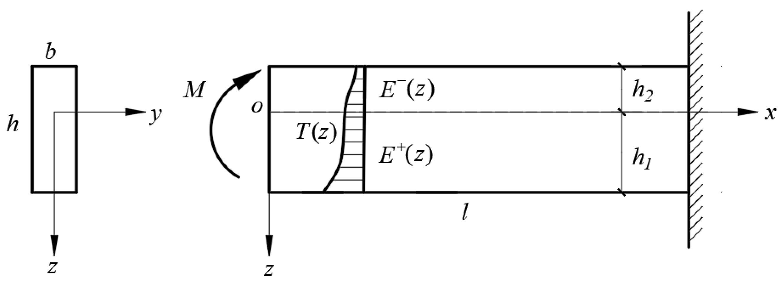
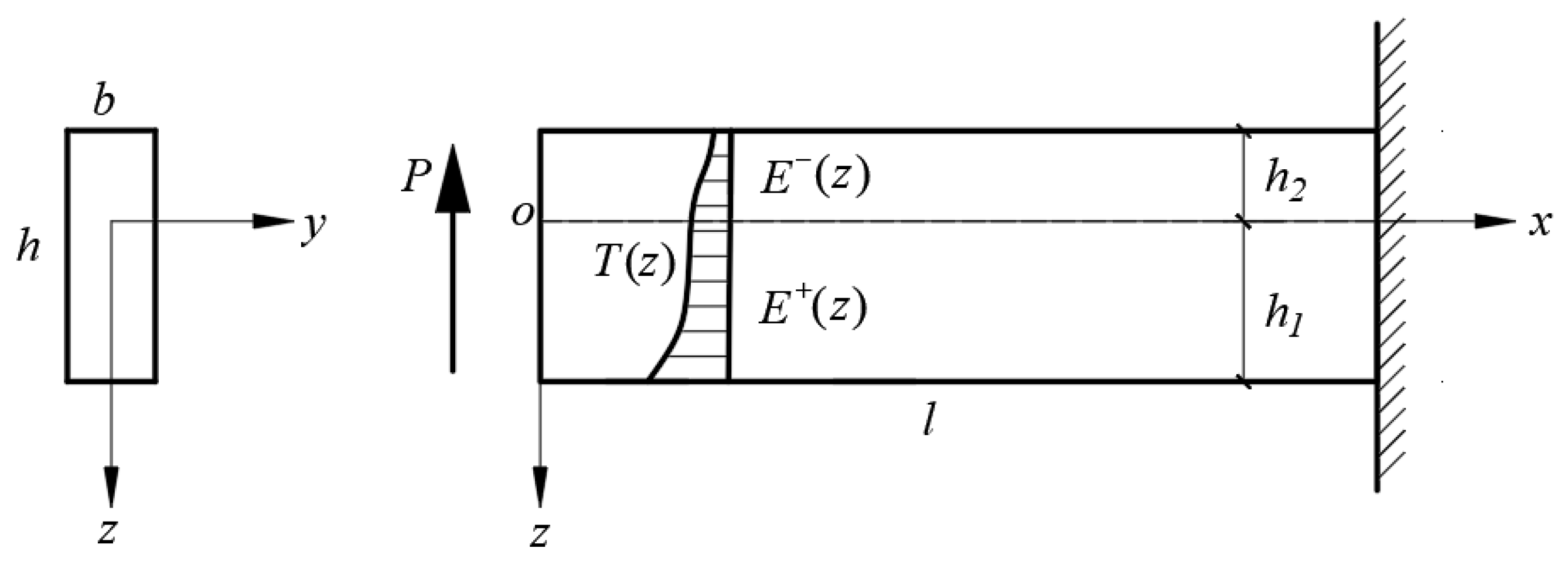
3.2. Lateral-Force Bending

Let us analyze a bimodular FGM cantilever beam under thermal load and a concentrated force on the end, P, as shown in Figure 4, in which the meaning of other physical quantities may refer to the previous definitions.

Due to [1]

$${\sigma }_z^{+/-}=\frac{{\partial }^2{\phi }^{+/-}(x, z)}{\partial x^2}=0,$$

(39)

we may have the stress function as, by integration,

$${\phi }^{+/-}(x, z)=x{f}^{+/-}(z)+f_1{}^{+/-}(z),$$

(40)

in which f ^+/−(z) and f ₁^+/−(z) are two unknown functions of z, which may be determined via a compatibility equation. Substituting Equation (40) into Equations (15) and (16), we have the stress

$$\{\begin{array}{l}{\sigma }_x^{+/-}=\frac{{\partial }^2{\phi }^{+/-}}{\partial z^2}=x\frac{d^2{f}^{+/-}(z)}{d{z}^2}+\frac{d^2{f}_1^{+/-}(z)}{d{z}^2}\hfill \\ {\sigma }_z^{+/-}=\frac{{\partial }^2{\phi }^{+/-}}{\partial x^2}=0\hfill \\ {\tau }_{xz}^{+/-}=-\frac{{\partial }^2{\phi }^{+/-}}{\partial x\partial z}=-\frac{d{f}^{+/-}(z)}{dz}\hfill \end{array},$$

(41)

and the strain

$$\{\begin{array}{l}{\epsilon }_x=\frac{1}{E_0{e}^{a_{i}z/h}}\left(x\frac{d^2{f}^{+/-}(z)}{d{z}^2}+\frac{d^2{f}_1^{+/-}(z)}{d{z}^2}\right)+{\alpha }_0{e}^{cz/h}T\\ {\epsilon }_z=-\frac{\mu }{E_0{e}^{a_{i}z/h}}\left(x\frac{d^2{f}^{+/-}(z)}{d{z}^2}+\frac{d^2{f}_1^{+/-}(z)}{d{z}^2}\right)+{\alpha }_0{e}^{cz/h}T\\ {\gamma }_{xz}=-\frac{2\left(1+\mu \right)}{E_0{e}^{a_{i}z/h}}\frac{d{f}^{+/-}(z)}{dz}\end{array}.$$

(42)

Substituting the above strain into Equation (13), we have

$$\frac{d^2}{d{z}^2}\left[\frac{1}{E_0{e}^{a_{i}z/h}}\left(x\frac{d^2{f}^{+/-}(z)}{d{z}^2}+\frac{d^2{f}_1^{+/-}(z)}{d{z}^2}\right)+{\alpha }_0{e}^{cz/h}T\right]=0,$$

(43)

which is a linear equation with respect to x. Since all x should satisfy Equation (43), the coefficients of x and x⁰ should be zero, thus resulting in

$$\frac{d^2}{d{z}^2}\left[\frac{1}{E_0{e}^{a_{i}z/h}}\frac{d^2{f}^{+/-}(z)}{d{z}^2}\right]=0,$$

(44)

$$\frac{d^2}{d{z}^2}\left[\frac{1}{E_0{e}^{a_{i}z/h}}\frac{d^2{f}_1^{+/-}(z)}{d{z}^2}+{\alpha }_0{e}^{cz/h}T\right]=0.$$

(45)

Integrating Equation (44) with respect to z continuously, we have

$$\frac{d^2{f}^{+/-}(z)}{d{z}^2}=(C_1^{+/-}z+C_2^{+/-})E_0{e}^{a_{i}z/h},$$

(46)

$$\frac{d{f}^{+/-}(z)}{dz}=\left(z-\frac{h}{{\alpha }_i}\right)\frac{C_1^{+/-}h{E}_0{e}^{a_{i}z/h}}{{\alpha }_i}+\frac{C_2^{+/-}h{E}_0{e}^{a_{i}z/h}}{{\alpha }_i}+C_3^{+/-},$$

(47)

$$f^{+/-}(z)=\left(z-\frac{2h}{{\alpha }_i}\right)\frac{C_1^{+/-}{h}^2{E}_0{e}^{a_{i}z/h}}{{\alpha }_i^2}+\frac{C_2^{+/-}{h}^2{E}_0{e}^{a_{i}z/h}}{{\alpha }_i^2}+C_3^{+/-}z+C_4^{+/-},$$

(48)

in which C₁^+/−, C₂^+/−, C₃^+/− and C₄^+/− are eight unknown integration constants. Similarly, integrating Equation (45) with respect to z continuously, also noting T = T(z), we have

$$\frac{d^2{f}_1^{+/-}(z)}{d{z}^2}=\left(C_5^{+/-}z+C_6^{+/-}-{\alpha }_0{e}^{cz/h}T\right)E_0{e}^{a_{i}z/h},$$

(49)

$$\frac{d{f}_1^{+/-}(z)}{dz}=\left(z-\frac{h}{a_i}\right)\frac{C_5^{+/-}h{E}_0{e}^{a_{i}z/h}}{a_i}+\frac{C_6^{+/-}h{E}_0{e}^{a_{i}z/h}}{a_i}-{\displaystyle \int E_0{\alpha }_0{e}^{\left(a_i+c\right)z/h}Tdz}+C_7^{+/-},$$

(50)

$$\begin{array}{l}{f}_1^{+/-}(z)=\left(z-\frac{2h}{a_i}\right)\frac{C_5^{+/-}{h}^2{E}_0{e}^{a_{i}z/h}}{a_i^2}+\frac{C_6^{+/-}{h}^2{E}_0{e}^{a_{i}z/h}}{a_i^2}\\ \hspace{1em}\hspace{1em}\hspace{1em}-{\displaystyle \int \left({\displaystyle \int E_0{\alpha }_0{e}^{\left(a_i+c\right)z/h}Tdz}\right)}dz+C_7^{+/-}z+C_8^{+/-}\end{array},$$

(51)

in which C₅^+/−, C₆^+/−, C₇^+/− and C₈^+/− are eight unknown integration constants. Note that C₄^+/− in f ^+/−(z), as well as C₇^+/− and C₈^+/− in f ₁^+/−(z), may be ignored in the stress function ϕ^+/−(x,z); thus, we have

$$\begin{array}{l}{\phi }^{+/-}=x\left[\left(z-\frac{2h}{{\alpha }_i}\right)\frac{C_1^{+/-}{h}^2{E}_0{e}^{{\alpha }_{i}z/h}}{{\alpha }_i^2}+\frac{C_2^{+/-}{h}^2{E}_0{e}^{{\alpha }_{i}z/h}}{{\alpha }_i^2}+C_3^{+/-}z\right]\\ \hspace{1em}+\left(z-\frac{2h}{a_i}\right)\frac{C_5^{+/-}{h}^2{E}_0{e}^{a_{i}z/h}}{a_i^2}+\frac{C_6^{+/-}{h}^2{E}_0{e}^{a_{i}z/h}}{a_i^2}-{\displaystyle \int \left({\displaystyle \int E_0{\alpha }_0{e}^{\left(a_i+c\right)z/h}Tdz}\right)}dz\end{array}.$$

(52)

Substituting Equation (52) into Equation (41), we have the stress components containing C₁^+/−, C₂^+/−, C₃^+/−, C₅^+/− and C₆^+/− as follows:

$$\{\begin{array}{l}{\sigma }_x^{+/-}=\frac{{\partial }^2{\phi }^{+/-}}{\partial z^2}=x\left(C_1^{+/-}z+C_2^{+/-}\right)E_0{e}^{a_{i}z/h}+\left(C_5^{+/-}z+C_6^{+/-}-{\alpha }_0{e}^{cz/h}T\right)E_0{e}^{a_{i}z/h}\hfill \\ {\sigma }_z^{+/-}=\frac{{\partial }^2{\phi }^{+/-}}{\partial x^2}=0\hfill \\ {\tau }_{xz}^{+/-}=-\frac{{\partial }^2{\phi }^{+/-}}{\partial x\partial z}=-\left(z-\frac{h}{a_i}\right)\frac{C_1^{+/-}h{E}_0{e}^{a_{i}z/h}}{a_i}-\frac{C_2^{+/-}h{E}_0{e}^{a_{i}z/h}}{a_i}-C_3^{+/-}\hfill \end{array}.$$

(53)

Next, the boundary conditions on the four sides of the beam and continuity conditions on the neutral layer (z = 0) will be used for the determination of C₁^+/−, C₂^+/−, C₃^+/−, C₅^+/− and C₆^+/−.

First, at z = 0, the continuity conditions, which are the same as Equation (26), still hold. Applying this to σ_x^+/− in Equation (53), we need to satisfy

$${\sigma }_x^{+}=x{C}_2^{+}{E}_0+C_6^{+}{E}_0-{\alpha }_{0}T{E}_0={\sigma }_x^{-}=x{C}_2^{-}{E}_0+C_6^{-}{E}_0-{\alpha }_{0}T{E}_0.$$

(54)

Obviously, we have

$$C_2^{+}=C_2^{-}, C_6^{+}=C_6^{-}.$$

(55)

In addition, according to the definition for the neutral axis of a bimodular problem, the strain here should be zero, that is, the same condition as Equation (29) also holds true. Combining the first part of Equation (42), as well as Equations (46) and (49), at z = 0, we have

$$\{\begin{array}{l}{\epsilon }_x^{+}=\frac{1}{E_0}\left(x{C}_2^{+}{E}_0+C_6^{+}{E}_0-{\alpha }_{0}T{E}_0\right)+{\alpha }_{0}T\\ {\epsilon }_x^{-}=\frac{1}{E_0}\left(x{C}_2^{-}{E}_0+C_6^{-}{E}_0-{\alpha }_{0}T{E}_0\right)+{\alpha }_{0}T\end{array}.$$

(56)

According to Equation (29), we obtain

$$C_2^{+}=C_2^{-}=C_6^{+}=C_6^{-}=0.$$

(57)

Thus, the τ_xy^+/− in Equation (53) may be simplified as

$$\{\begin{array}{l}{\tau }_{xz}^{+}=-\left(z-\frac{h}{a_1}\right)\frac{C_1^{+}h{E}_0{e}^{a_{1}z/h}}{a_1}-C_3^{+}\\ {\tau }_{xz}^{-}=-\left(z-\frac{h}{a_2}\right)\frac{C_1^{-}h{E}_0{e}^{a_{2}z/h}}{a_2}-C_3^{-}\end{array}.$$

(58)

Note that at z = 0, we have the continuity condition [35], τ_xz⁺ = τ_xz⁻, thus we have

$$\frac{C_1^{+}{h}^2{E}_0}{a_1^2}-C_3^{+}=\frac{C_1^{-}{h}^2{E}_0}{a_2^2}-C_3^{-},$$

(59)

which gives the first relation among C₁^+/− and C₃^+/−.

Now, let us consider the boundary conditions on the four sides. First, on the two main sides, we still have the boundary conditions which are the same as Equation (32). Applying the boundary conditions of τ_xy^+/− to Equation (58), we have

$$\{\begin{array}{l}{\tau }_{xz}^{+}=-\left(h_1-\frac{h}{a_1}\right)\frac{C_1^{+}h{E}_0{e}^{a_{1}z/h}}{a_1}-C_3^{+}=0, \mathrm{at} z=h_1\\ {\tau }_{xz}^{-}=-\left(-h_2-\frac{h}{a_2}\right)\frac{C_1^{-}h{E}_0{e}^{-a_2{h}_2/h}}{a_2}-C_3^{-}=0, \mathrm{at} z=-h_2\end{array},$$

(60)

which gives another two relations among C₁^+/− and C₃^+/−. Obviously, Equations (59) and (60) are still insufficient to solve the four constants C₁^+/− and C₃^+/−. Due to l >> h, at x = 0, we may apply the Saint-Venant principle to obtain three integration equations; this yields

$$\{\begin{array}{l}{\displaystyle {\int }_{-h_2}^0{\sigma }_x^{-}}dz+{\displaystyle {\int }_0^{h_1}{\sigma }_x^{+}}dz=0\hfill \\ {\displaystyle {\int }_{-h_2}^0{\sigma }_x^{-}}zdz+{\displaystyle {\int }_0^{h_1}{\sigma }_x^{+}}zdz=0\hfill \\ {\displaystyle {\int }_{-h_2}^0{\tau }_{xz}^{-}}dz+{\displaystyle {\int }_0^{h_1}{\tau }_{xz}^{+}}dz=\frac{P}{b}\hfill \end{array}.$$

(61)

Substituting τ_xz^+/− of Equation (58) into the third part of Equation (61), we have

$${\displaystyle {\int }_{-h_2}^0\left[\left(z-\frac{h}{a_2}\right)\frac{C_1^{-}h{E}_0{e}^{a_{2}z/h}}{a_2}+C_3^{-}\right]}dz+{\displaystyle {\int }_0^{h_1}\left[\left(z-\frac{h}{a_1}\right)\frac{C_1^{+}h{E}_0{e}^{a_{1}z/h}}{a_1}+C_3^{+}\right]}dz=-\frac{P}{b},$$

(62)

which gives the fourth relation containing C₁^+/− and C₃^+/−. Combining Equations (59), (60) and (62), after a complicated solving, we obtain (for details, please see Appendix A)

$$\{\begin{array}{l}{C}_1^{+}=-\frac{P}{b{E}_0}\frac{-A_1^{-}}{A_2^{+}{A}_1^{-}-A_2^{-}{A}_1^{+}}\\ C_1^{-}=-\frac{P}{b{E}_0}\frac{A_1^{+}}{A_2^{+}{A}_1^{-}-A_2^{-}{A}_1^{+}}\\ C_3^{+}=\frac{P}{b}\frac{-A_1^{-}}{A_2^{+}{A}_1^{-}-A_2^{-}{A}_1^{+}}\left(h_1-\frac{h}{{\alpha }_1}\right)\frac{h{e}^{{\alpha }_1{h}_1/h}}{{\alpha }_1}\\ C_3^{-}=\frac{P}{b}\frac{A_1^{+}}{A_2^{+}{A}_1^{-}-A_2^{-}{A}_1^{+}}\left(-h_2-\frac{h}{{\alpha }_2}\right)\frac{h{e}^{-{\alpha }_2{h}_2/h}}{{\alpha }_2}\end{array}.$$

(63)

Up to now, C₁^+/−, C₂^+/−, C₃^+/− and C₆^+/− have been determined, and only C₅^+/− are unknown. For this purpose, at x = 0, we first have the σ_x^+/− according to Equation (53):

$${\sigma }_x^{+}=\left(C_5^{+}z-{\alpha }_0{e}^{cz/h}T\right)E_0{e}^{a_{1}z/h}, {\sigma }_x^{-}=\left(C_5^{-}z-{\alpha }_0{e}^{cz/h}T\right)E_0{e}^{a_{2}z/h}.$$

(64)

Substituting it into the former two of Equation (61), we have

$$\{\begin{array}{l}{\displaystyle {\int }_0^{h_1}\left[\left(C_5^{+}z-{\alpha }_0{e}^{cz/h}T\right)E_0{e}^{a_{1}z/h}\right]}dz+{\displaystyle {\int }_{-h_2}^0\left[\left(C_5^{-}z-{\alpha }_0{e}^{cz/h}T\right)E_0{e}^{a_{2}z/h}\right]}dz=0\\ {\displaystyle {\int }_0^{h_1}\left[\left(C_5^{+}z-{\alpha }_0{e}^{cz/h}T\right)E_0{e}^{a_{1}z/h}\right]}zdz+{\displaystyle {\int }_{-h_2}^0\left[\left(C_5^{-}z-{\alpha }_0{e}^{cz/h}T\right)E_0{e}^{a_{2}z/h}\right]}zdz=0\end{array},$$

(65)

which gives

$$\{\begin{array}{l}{C}_5^{+}{A}_1^{+}+C_5^{-}{A}_1^{-}={\alpha }_0(T_0^{+}+T_0^{-})\\ C_5^{+}{A}_2^{+}+C_5^{-}{A}_2^{-}={\alpha }_0(T_1^{+}+T_1^{-})\end{array},$$

(66)

in which, A₁^+/−, A₂^+/−, T₀^+/− and T₁^+/− are respectively shown in Equation (7). From Equation (66), we solve

$$\{\begin{array}{l}{C}_5^{+}=-\frac{A_1^{-}{\alpha }_0(T_1^{+}+T_1^{-})-A_2^{-}{\alpha }_0(T_0^{+}+T_0^{-})}{A_1^{+}{A}_2^{-}-A_1^{-}{A}_2^{+}}\\ C_5^{-}=\frac{A_1^{+}{\alpha }_0(T_1^{+}+T_1^{-})-A_2^{+}{\alpha }_0(T_0^{+}+T_0^{-})}{A_1^{+}{A}_2^{-}-A_1^{-}{A}_2^{+}}\end{array}.$$

(67)

Finally, we obtain the stress component, as follows:

$$\begin{array}{l}\{\begin{array}{l}{\sigma }_x^{+}=\frac{P}{b}\frac{A_1^{-}}{A_2^{+}{A}_1^{-}-A_2^{-}{A}_1^{+}}xz{e}^{a_{1}z/h}-\left[\frac{A_1^{-}(T_1^{+}+T_1^{-})-A_2^{-}(T_0^{+}+T_0^{-})}{A_1^{+}{A}_2^{-}-A_1^{-}{A}_2^{+}}z+e^{cz/h}T\right]{\alpha }_0{E}_0{e}^{a_{1}z/h}\hfill \\ {\sigma }_z^{+}=0 \hspace{1em}\hspace{1em}\hspace{1em}\hspace{1em}\hspace{1em}\hspace{1em}\hspace{1em}\hspace{1em}\hspace{1em}\hspace{1em}\hspace{1em}\hspace{1em}\hspace{1em}\hspace{1em}\hspace{1em}\hspace{1em}\hspace{1em}\hspace{1em}\hspace{1em}\mathrm{at}0\le z\le h_1 \hfill \\ {\tau }_{xz}^{+}=-\frac{P}{b}\frac{A_1^{-}}{A_2^{+}{A}_1^{-}-A_2^{-}{A}_1^{+}}\left(z-\frac{h}{a_1}\right)\frac{h{e}^{a_{1}z/h}}{a_1}+\frac{P}{b}\frac{A_1^{-}}{A_2^{+}{A}_1^{-}-A_2^{-}{A}_1^{+}}\left(h_1-\frac{h}{{\alpha }_1}\right)\frac{h{e}^{{\alpha }_1{h}_1/h}}{{\alpha }_1}\hfill \end{array}\\ \{\begin{array}{l}{\sigma }_x^{-}=-\frac{P}{b}\frac{A_1^{+}}{A_2^{+}{A}_1^{-}-A_2^{-}{A}_1^{+}}xz{e}^{a_{2}z/h}+\left[\frac{A_1^{+}(T_1^{+}+T_1^{-})-A_2^{+}(T_0^{+}+T_0^{-})}{A_1^{+}{A}_2^{-}-A_1^{-}{A}_2^{+}}z-e^{cz/h}T\right]{\alpha }_0{E}_0{e}^{a_{2}z/h}\hfill \\ {\sigma }_z^{-}=0 \hspace{1em}\hspace{1em}\hspace{1em}\hspace{1em}\hspace{1em}\hspace{1em}\hspace{1em}\hspace{1em}\hspace{1em}\hspace{1em}\hspace{1em}\hspace{1em}\hspace{1em}\hspace{1em}\hspace{1em}\hspace{1em}\hspace{1em}\hspace{1em}\hspace{1em}\mathrm{at}-h_2\le z\le 0\hfill \\ {\tau }_{xz}^{-}=\frac{P}{b}\frac{A_1^{+}}{A_2^{+}{A}_1^{-}-A_2^{-}{A}_1^{+}}\left(z-\frac{h}{a_2}\right)\frac{h{e}^{a_{2}z/h}}{a_2}+\frac{P}{b}\frac{A_1^{+}}{A_2^{+}{A}_1^{-}-A_2^{-}{A}_1^{+}}\left(h_2+\frac{h}{{\alpha }_2}\right)\frac{h{e}^{-{\alpha }_2{h}_2/h}}{{\alpha }_2}\hfill \end{array}\end{array}$$

(68)

4. Comparisons and Regression

4.1. Comparison of Two-Dimensional Pure Bending and Lateral-Force Bending Solutions

The two-dimensional thermoelastic solutions under pure bending and lateral-force bending are shown in Equations (38) and (68), respectively. By observing the two sets of equations, it is easy to find that with the exception of the term concerning external loads, all other terms are the same. For this purpose, we only take the term concerning external loads from the two sets of equations. For the pure bending, the stress from the bending moment M is

$$\{\begin{array}{l}{\sigma }_{x, M}^{+}=\frac{-A_1^{-}}{A_1^{+}{A}_2^{-}-A_1^{-}{A}_2^{+}}\frac{M}{b}z{e}^{a_{1}z/h}, \mathrm{at} 0\le z\le h_1\hfill \\ {\sigma }_{x, M}^{-}=\frac{A_1^{+}}{A_1^{+}{A}_2^{-}-A_1^{-}{A}_2^{+}}\frac{M}{b}z{e}^{a_{2}z/h}, \mathrm{at}-h_2\le z\le 0\hfill \end{array},$$

(69)

while for the lateral-force bending, the stress from the concentrated force P is

$$\{\begin{array}{l}{\sigma }_{x, P}^{+}=\frac{P}{b}\frac{A_1^{-}}{A_1^{+}{A}_2^{-}-A_1^{-}{A}_2^{+}}xz{e}^{a_{1}z/h}, \mathrm{at} 0\le z\le h_1\hfill \\ {\sigma }_{x, P}^{-}=\frac{P}{b}\frac{-A_1^{+}}{A_1^{+}{A}_2^{-}-A_1^{-}{A}_2^{+}}xz{e}^{a_{2}z/h}, \mathrm{at}-h_2\le z\le 0\hfill \end{array}.$$

(70)

Obviously, if we let

$$M=-Px,$$

(71)

which may be easily obtained from Figure 4, Equations (69) and (70) are exactly the same. This agreement indicates that two-dimensional thermoelastic stress solutions under pure bending and lateral-force bending are consistent in essence; this is due to the following two facts. One is that the two solutions are obtained under the stress function method based on the compatibility condition. Another fact that should be noted here that is during the solving, the application of the boundary conditions and continuity conditions is basically the same. Unfortunately, shear stresses cannot be compared, since there is no shear stress under pure bending. Given that two-dimensional solutions under pure bending and lateral-force bending are the same, in the next comparison of one- and two-dimensional solutions, we take the solution under pure bending.

4.2. Comparison of One- and Two-Dimensional Pure Bending Solutions

The one- and two-dimensional stress solutions under pure bending are shown in Equations (10) and (38), respectively. From the formulae, it can be observed that the thermal stress consists of three parts: temperature stresses due to strain suppression σ_x,s = −α(z)E(z)T(z), axial stresses σ_x,a, and bending stresses σ_x,b, in which the axial and bending stresses may come from two different origins—one from strain suppression and the other from externally applied loads. From Equations (10) and (38), it is easy to see that in the one- and two-dimensional stress solutions, the temperature stresses due to strain suppression are the same, which gives

$$\{\begin{array}{l}{\sigma }_{x, s}^{+}=-{\alpha }_0{e}^{cz/h}{E}_0{e}^{a_{1}z/h}T(z), \mathrm{at} 0\le z\le h_1\hfill \\ {\sigma }_{x, s}^{-}=-{\alpha }_0{e}^{cz/h}{E}_0{e}^{a_{2}z/h}T(z), \mathrm{at}-h_2\le z\le 0\hfill \end{array}.$$

(72)

Thus, our attention will focus on the axial stresses σ_x,a and bending stresses σ_x,b.

For the axial stresses σ_x,a, the one-dimensional stress solution, or Equation (10), gives

$$\{\begin{array}{l}{\sigma }_{x, a}^{+}=E_0{e}^{a_{1}z/h}\frac{{\alpha }_0(T_0^{+}+T_0^{-})}{A_0^{+}+A_0^{-}}, \mathrm{at} 0\le z\le h_1\hfill \\ {\sigma }_{x, a}^{-}=E_0{e}^{a_{2}z/h}\frac{{\alpha }_0(T_0^{+}+T_0^{-})}{A_0^{+}+A_0^{-}}, \mathrm{at}-h_2\le z\le 0\hfill \end{array},$$

(73)

while the two-dimensional stress solution, or Equation (38), gives

$$\{\begin{array}{l}{\sigma }_{x, a}^{+}=E_0{e}^{a_{1}z/h}\frac{A_2^{-}{\alpha }_0(T_0^{+}+T_0^{-})}{A_1^{+}{A}_2^{-}-A_1^{-}{A}_2^{+}}z, \mathrm{at} 0\le z\le h_1\hfill \\ {\sigma }_{x, a}^{-}=E_0{e}^{a_{2}z/h}\frac{-A_2^{+}{\alpha }_0(T_0^{+}+T_0^{-})}{A_1^{+}{A}_2^{-}-A_1^{-}{A}_2^{+}}z, \mathrm{at}-h_2\le z\le 0\hfill \end{array}.$$

(74)

Due to the relation A₁⁺ + A₁⁻ = 0, Equation (74) may be written as

$$\{\begin{array}{l}{\sigma }_{x, a}^{+}=-E_0{e}^{a_{1}z/h}\frac{{\alpha }_0(T_0^{+}+T_0^{-})}{A_2^{-}+A_2^{+}}\frac{A_2^{-}}{A_1^{-}}z, \mathrm{at} 0\le z\le h_1\hfill \\ {\sigma }_{x, a}^{-}=-E_0{e}^{a_{2}z/h}\frac{{\alpha }_0(T_0^{+}+T_0^{-})}{A_2^{-}+A_2^{+}}\frac{A_2^{+}}{A_1^{+}}z, \mathrm{at}-h_2\le z\le 0\hfill \end{array}.$$

(75)

From Equations (73) and (75), it is found that they are almost identical and the main difference is from the computation for strain. In the one-dimensional solution, the strain is a constant, which agrees with the basic characteristic of the one-dimensional problem. For a common shallow beam, the variation along the z direction is generally ignored or, alternatively, the one-dimensional solution can not reflect the change along the z direction. In the two-dimensional solution, the strain has not been a constant; it varies with the z direction and is a function of z. This fact is consistent with the basic feature of the two-dimensional problem. This difference will be discussed in the next section concerning the regression and validation of the solutions.

For the bending stresses σ_x,b, the one-dimensional stress solution, or Equation (10), gives

$$\{\begin{array}{l}{\sigma }_{x, b}^{+}=E_0{e}^{a_{1}z/h}z\frac{M/E_{0}b+{\alpha }_0(T_1{}^{+}+T_1{}^{-})}{A_2{}^{+}+A_2{}^{-}}, \mathrm{at} 0\le z\le h_1\hfill \\ {\sigma }_{x, b}^{-}=E_0{e}^{a_{2}z/h}z\frac{M/E_{0}b+{\alpha }_0(T_1{}^{+}+T_1{}^{-})}{A_2{}^{+}+A_2{}^{-}}, \mathrm{at}-h_2\le z\le 0\hfill \end{array},$$

(76)

while the two-dimensional stress solution, or Equation (38), gives

$$\{\begin{array}{l}{\sigma }_{x, b}^{+}=\frac{-A_1^{-}}{A_1^{+}{A}_2^{-}-A_1^{-}{A}_2^{+}}\left[\frac{M}{E_{0}b}+{\alpha }_0(T_1^{+}+T_1^{-})\right]z{E}_0{e}^{a_{1}z/h}, \mathrm{at} 0\le z\le h_1\hfill \\ {\sigma }_{x, b}^{-}=\frac{A_1^{+}}{A_1^{+}{A}_2^{-}-A_1^{-}{A}_2^{+}}\left[\frac{M}{E_{0}b}+{\alpha }_0(T_1^{+}+T_1^{-})\right]z{E}_0{e}^{a_{2}z/h}, \mathrm{at}-h_2\le z\le 0\hfill \end{array}.$$

(77)

If we note that the conditions for the determination of the neutral axis, that is, A₁⁺ + A₁⁻ = 0, Equation (77) will become

$$\{\begin{array}{l}{\sigma }_{x, b}^{+}=\frac{1}{A_2^{-}+A_2^{+}}\left[\frac{M}{E_{0}b}+{\alpha }_0(T_1^{+}+T_1^{-})\right]z{E}_0{e}^{a_{1}z/h}, \mathrm{at} 0\le z\le h_1\hfill \\ {\sigma }_{x, b}^{-}=\frac{1}{A_2^{-}+A_2^{+}}\left[\frac{M}{E_{0}b}+{\alpha }_0(T_1^{+}+T_1^{-})\right]z{E}_0{e}^{a_{2}z/h}, \mathrm{at}-h_2\le z\le 0\hfill \end{array}.$$

(78)

Obviously, Equation (78) is the same as Equation (76). This indicates that for the bending stresses σ_x,b, the one-dimensional solution is consistent with the two-dimensional solution.

4.3. Regression and Validation

Due to the fact that up to now, analytical solutions for the thermal stress of bimodular FGM beams have not been found in existing work, there is no similar problem that can be used for comparison with this study. In order to validate the accuracy of the present method, only under certain regression conditions—for example, the regression to the singular modulus problem—can we use other work to verify the solutions obtained in this study. For this purpose, if we let E⁺(z) = E⁻(z) = E(z) = E₀ e ^az/h, or a₁ = a₂ = a, at the same time, M = 0 if no external applied loads are considered, Equation (10) will become

$${\sigma }_x=E(z)\left[-\alpha (z)T(z)+\frac{{\displaystyle \int E_0{e}^{az/h}{\alpha }_0{e}^{cz/h}T(z)}dz}{{\displaystyle \int E_0{e}^{az/h}}dz}+\frac{{\displaystyle \int E_0{e}^{az/h}{\alpha }_0{e}^{cz/h}T(z)z}dz}{{\displaystyle \int E_0{e}^{az/h}{z}^2}dz}z\right].$$

(79)

It may also be further written as

$${\sigma }_x=E(z)\left[-\alpha (z)T(z)+\frac{{\displaystyle \int E(z)\alpha (z)T(z)}dz}{{\displaystyle \int E(z)}dz}+\frac{{\displaystyle \int E(z)\alpha (z)T(z)z}dz}{{\displaystyle \int E(z)z^2}dz}z\right],$$

(80)

On the other hand, the theory of elasticity by Timoshenko and Goodier [1] gives the thermal stress solution as

$${\sigma }_x=E\left(-\alpha T+\frac{{\displaystyle \int E\alpha Tdz}}{{\displaystyle \int Edz}}+z\frac{{\displaystyle \int E\alpha Tzdz}}{{\displaystyle \int E{z}^{2}dz}}\right),$$

(81)

in which E, α and T are the functions of z, that is, E = E(z), α = α(z) and T = T(z). It is easy to see that Equations (80) and (81) are the same, and this verifies the correctness of the solution obtained in this study from the side, although this validation is based on the regression to the singular modulus problem.

In addition, for a common material beam without the bimodular functionally graded characteristic, if we further let a₁ = a₂ = c = 0, and thus we have h₁ = h₂ = h/2, Equation (7) will be simplified as

$$\{\begin{array}{l}{A}_0{}^{+}={\displaystyle {\int }_0^{h/2}dz}=\frac{h}{2}, A_0{}^{-}={\displaystyle {\int }_{-h/2}^{0}dz}=\frac{h}{2}\\ A_1{}^{+}={\displaystyle {\int }_0^{h/2}z}dz=\frac{h^2}{8}, A_1{}^{-}={\displaystyle {\int }_{-h/2}^{0}z}dz=-\frac{h^2}{8}\\ A_2{}^{+}={\displaystyle {\int }_0^{h/2}{z}^2}dz=\frac{h^3}{24}, A_2{}^{-}={\displaystyle {\int }_{-h/2}^0{z}^2}dz=\frac{h^3}{24} \\ T_0^{+}={\displaystyle {\int }_0^{h/2}T(z)dz}, T_0^{-}={\displaystyle {\int }_{-h/2}^{0}T(z)dz}\\ T_1^{+}={\displaystyle {\int }_0^{h/2}T(z)zdz}, T_1^{-}={\displaystyle {\int }_{-h/2}^{0}T(z)zdz}\end{array}.$$

(82)

Thus, σ_x^+/− in Equation (10) will become

$${\sigma }_x=-{\alpha }_0{E}_{0}T(z)+\frac{1}{bh}{\displaystyle {\int }_{-h/2}^{h/2}{\alpha }_0{E}_{0}T(z)bdz+}\frac{z}{b{h}^3/12}\left(M+{\displaystyle {\int }_{-h/2}^{h/2}{\alpha }_0{E}_{0}T(z)bzdz}\right).$$

(83)

This is exactly the common thermal stress solution. While σ_x^+/− in Equation (38) will give

$${\sigma }_x^{\prime }=-{\alpha }_0{E}_{0}T(z)\pm \frac{4}{h^2}z{\displaystyle {\int }_{-h/2}^{h/2}{\alpha }_0{E}_{0}T(z)dz+}\frac{z}{b{h}^3/12}\left(M+{\displaystyle {\int }_{-h/2}^{h/2}{\alpha }_0{E}_{0}T(z)bzdz}\right).$$

(84)

in which ‘+’ for the range of 0 < z < h/2, and ‘−’ for −h/2 < z < 0. Again, it is found that differences only exist in the axial stress, to some extent. The axial stress in Equations (83) and (84) gives, respectively,

$${\sigma }_{x, a}=\frac{1}{bh}{\displaystyle {\int }_{-h/2}^{h/2}{\alpha }_0{E}_{0}T(z)bdz}.$$

(85)

and

$${\sigma }_{x, a}^{\prime }=\pm \frac{4}{h^2}z{\displaystyle {\int }_{-h/2}^{h/2}{\alpha }_0{E}_{0}T(z)dz}.$$

(86)

Now, let us sum up their resultants on the whole cross-section. First, for Equation (85), we have the resultant R:

$$R={\displaystyle {\int }_{-h/2}^{h/2}{\alpha }_0{E}_{0}T(z)bdz},$$

(87)

and for Equation (86),

$$\begin{array}{l}{R}^{\prime }=\frac{4}{h^2}{\displaystyle {\int }_0^{h/2}zdz}{\displaystyle {\int }_{-h/2}^{h/2}{\alpha }_0{E}_{0}T(z)dz}-\frac{4}{h^2}{\displaystyle {\int }_{-h/2}^{0}zdz}{\displaystyle {\int }_{-h/2}^{h/2}{\alpha }_0{E}_{0}T(z)dz}\\ \hspace{1em}=\frac{1}{2}{\displaystyle {\int }_{-h/2}^{h/2}{\alpha }_0{E}_{0}T(z)dz}+\frac{1}{2}{\displaystyle {\int }_{-h/2}^{h/2}{\alpha }_0{E}_{0}T(z)dz}\\ \hspace{1em}={\displaystyle {\int }_{-h/2}^{h/2}{\alpha }_0{E}_{0}T(z)dz}\end{array},$$

(88)

in which the thickness of the beam b is regarded as unit 1, as assumed in the elasticity problem. It is obvious that the two resultants are the same, which indicates that the difference caused by the axial stress is generally small, and again verifies the correctness of the solution from the side.

5. Numerical Results and Discussions

5.1. Neutral Layer in Two Bimodular Cases

Note that the functionally graded materials with bimodular effect in this study are defined as, in the tensile zone, $E^{+}(z)=E_0{e}^{a_{1}z/h}$ for $0\le z\le h_1$, and in the compressive zone, $E^{-}(z)=E_0{e}^{a_{2}z/h}$ for $-h_2\le z\le 0$, in which a₁ and a₂ are two dimensionless grade parameters. We note the fact that, if the positive or negative signs of a₁ and a₂ are correctly selected, the relation among the tensile modulus E⁺(z), the compressive modulus E⁻(z) and the neutral layer modulus E₀ is definite. Basically, there are two bimodular cases: (a) a₁ > 0, a₂ > 0 and (b) a₁ < 0, a₂ < 0, respectively, which correspond to two cases of tensile and compressive moduli, that is, (a) E⁺(z) > E₀ > E⁻(z) and (b) E⁺(z) < E₀ < E⁻(z), as shown in Figure 5, in which the curve of E⁺(z) is represented in the solid lines and the curve of E⁻(z) in the dashed lines.

For the convenience of the analysis of the bimodular effect on the results, we select three groups of data of a₁ and a₂ for the cases (a) and (b); thus, there are data for a total of six groups, which are listed in

Table 1. Neutral layers in two cases as well as the classical case without bimodular functionally graded property.

Cases	Case (a) ${\mathit{E}}^{+}(\mathit{z})>{\mathit{E}}_0>{\mathit{E}}^{-}(\mathit{z})$			Case (b) ${\mathit{E}}^{+}(\mathit{z})<{\mathit{E}}_0<{\mathit{E}}^{-}(\mathit{z})$			Case (c) ${\mathit{E}}^{+}(\mathit{z})={\mathit{E}}^{-}(\mathit{z})={\mathit{E}}_0$
	$\begin{array}{l}{\mathit{a}}_1=3\\ {\mathit{a}}_2=1\end{array}$	$\begin{array}{l}{\mathit{a}}_1=2\\ {\mathit{a}}_2=1\end{array}$	$\begin{array}{l}{\mathit{a}}_1=1\\ {\mathit{a}}_2=1\end{array}$	$\begin{array}{l}{\mathit{a}}_1=-3\\ {\mathit{a}}_2=-1\end{array}$	$\begin{array}{l}{\mathit{a}}_1=-2\\ {\mathit{a}}_2=-1\end{array}$	$\begin{array}{l}{\mathit{a}}_1=-1\\ {\mathit{a}}_2=-1\end{array}$	$\begin{array}{l}{\mathit{a}}_1=0\\ {\mathit{a}}_2=0\end{array}$
h1/h	0.3585	0.3859	0.4181	0.6732	0.6277	0.5824	0.5
h2/h	0.6415	0.6141	0.5819	0.3268	0.3723	0.4176	0.5

. In addition, further data, a₁ = a₂ = 0, which corresponds to the classical problem without the bimodular functionally graded property, is also selected as an effective comparison. By using the given a₁ and a₂, we may compute the h₁/h and h₂/h via the formulas A₁⁺ + A₁⁻ = 0, that is,

$${\displaystyle {\int }_0^{h_1}{e}^{a_{1}z/h}z}dz+{\displaystyle {\int }_{-h_2}^0{e}^{a_{2}z/h}z}dz=0,$$

(89)

which further gives

$$\left(\frac{h_1}{a_1}-\frac{h}{a_1^2}\right)e^{a_1{h}_1/h}+\left(\frac{h_2}{a_2}+\frac{h}{a_2^2}\right)e^{-a_2{h}_2/h}=\frac{h}{a_2^2}-\frac{h}{a_1^2}.$$

(90)

Obviously, for the classical problem, not referring to Equation (90), it is readily known that h₁/h = h₂/h = 0.5, as shown in Table 1.

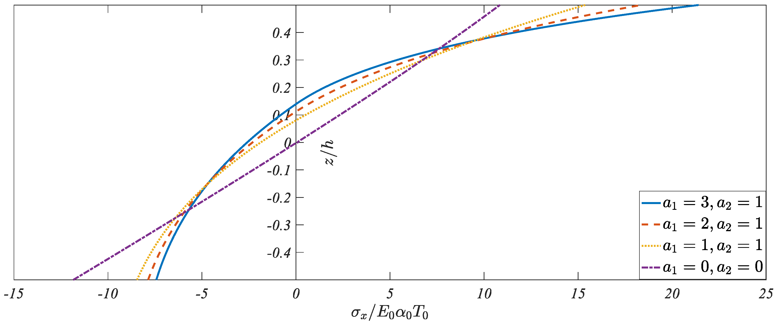
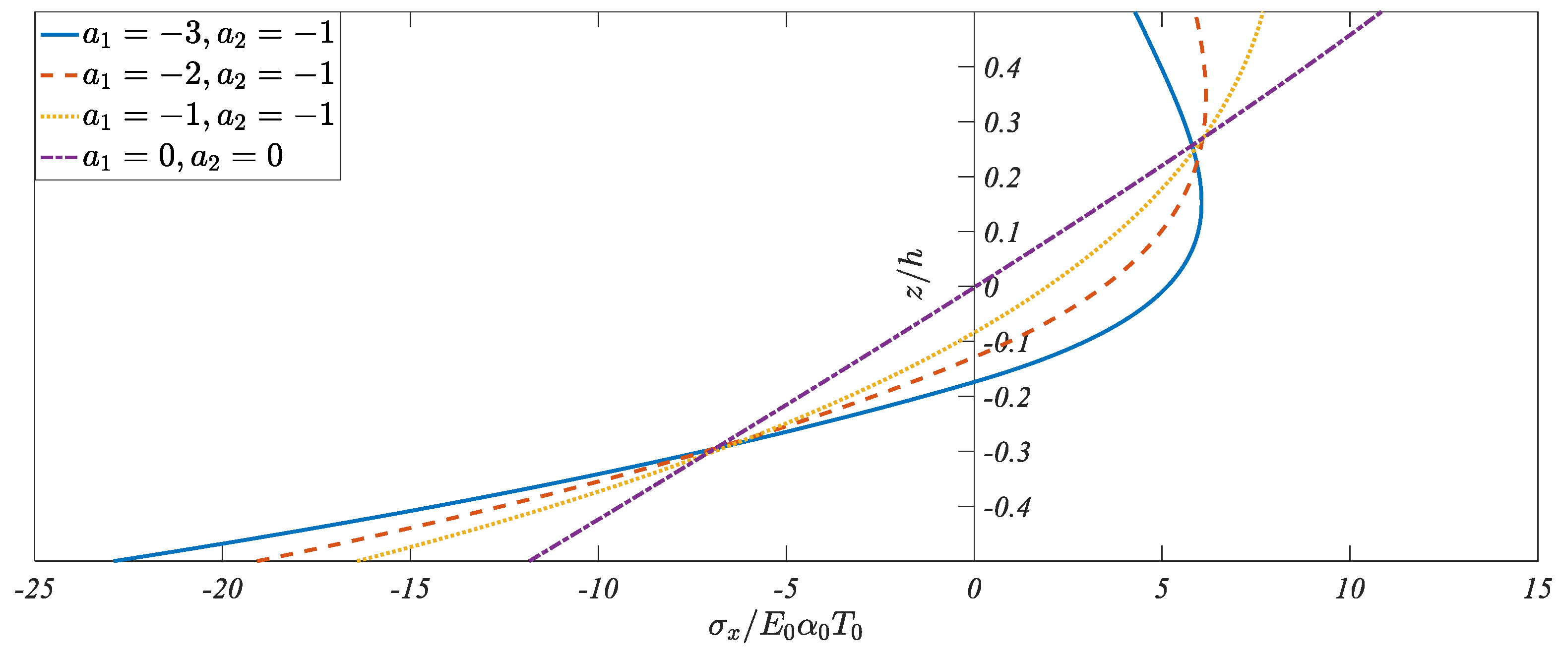
5.2. Axial Stresses in Two Bimodular Cases

From the comparison from Section 4.2, we know that the main difference between the one- and two-dimensional solutions lies in the axial stress. For this purpose, we plot the dimensionless variation curves of the axial stress with the z direction, as shown in Figure 6, Figure 7 and Figure 8, in which the horizontal coordinate, σ_x/E₀α₀T₀, represents the dimensionless axial stress, and the longitudinal coordinate, z/h, represents the dimensionless height. In Figure 6, Figure 7 and Figure 8, the parameter c in the line expansion coefficients α(z) is taken as c = 1. Figure 6 and Figure 7 are the axial stress comparison (Equations (73) and (75)) in two bimodular cases, while Figure 8 is for the classical case without the bimodular functionally graded property (Equations (85) and (86)). We also note that in Figure 6, Figure 7 and Figure 8, h₁/h and h₂/h are different. For Figure 6, the variation range of z is from −0.6141 to 0.3859; please refer to Table 1. For Figure 7, the variation range of z is from −0.3723 to 0.6277, while for Figure 8, the variation range of z is from −0.5 to 0.5, as we expected. In addition, the temperature rise mode is prescribed as T(z) = T₀ e ^cz/h, where c = 1.

From Figure 6, Figure 7 and Figure 8, it is easy to see that:

(i) All of the curve shapes agree with the real function forms. Specifically, Equation (73) is the exponential function of z, while Equation (73) presents the product of z and the exponential function of z, like the form ze^az/h. At the same time, Equation (85) is a constant and Equation (86) is a linear function of z, which agree well with the real curve shapes.

(ii) Although the variation of the axial stress with z is different, their resultants on the whole cross-section are equal. In Figure 6, Figure 7 and Figure 8, the resultant of the axial stress on the cross-section may be explained geometrically as the area formed by the axial stress curve and the horizontal boundary lines. It is easy to find that, especially for Figure 8, area B is equal to the sum of areas A and C, which verifies the equipotency of the resultant forces.

5.3. Bimodular Functionally Graded Effect on Thermal Stress

Now that, via the above comparison, it is concluded that the one- and two-dimensional solutions are consistent, we may analyze the bimodular functional-grade effect on the thermal stress using the one-dimensional solution shown in Equation (10) directly. Figure 9 and Figure 10 show the thermal stress variations in Equation (10) under cases (a) E⁺(z) > E⁻(z) and case (b) E⁺(z) > E⁻(z), in which four groups of data from a₁ and a₂ are considered, including the classical problem on a₁ = a₂ = 0; the temperature rise mode is prescribed as T(z) = T₀ e ^cz/h, where c = 1. Note that there is the bending moment M in Equation (10), thus, the relative magnitude of M and E₀α₀T₀ must be given in advance, otherwise the curves cannot be plotted. For this purpose, after considering the dimension of M, we prescribe the relative relation M/bh² = 2E₀α₀T₀.

From Figure 9 and Figure 10, it is easy to see that:

(i) When E⁺(z) > E⁻(z), the tensile stress in the beam is fully developed on the cross-section, resulting in the tensile stress being greater than the compressive stress. This phenomenon is well illustrated in Figure 9. A similar feature may also be found in Figure 10 when E⁺(z) < E⁻(z), the compressive stress in the beam, is fully developed, which is obviously greater than the tensile stress.

(ii) Generally speaking, the stress at the top and bottom of the beam tends to the maximum, while the stress at the neutral layer tends to the minimum. The introduction of a bimodular functionally graded property does not change this feature; however, there is still an exception that when E⁺(z) < E⁻(z), in the case of a₁ = −3 and a₂ = −1, the maximum tensile stress occurs on a certain layer along the horizontal direction, but not on the top or bottom layer of the beam.

(iii) The introduction of bimodular functionally graded property will further strengthen the nonlinearity of the problem. In the case a₁ = 0 and a₂ = 0, the variation curve approaches linear, although the temperature rise mode T(z) = T₀e ^z/h presents as nonlinear, to some extent. However, with the increase of the absolute values of the gradient parameters a₁ and a₂, the nonlinear characteristic becomes more obvious. The maximum stress, tensile or compressive, increases dramatically, in which for E⁺(z) > E⁻(z), the maximum tensile stress increases dramatically at the top layer of the beam while for E⁺(z) < E⁻(z), the maximum compressive stress increases dramatically at the bottom layer of the beam.

6. Concluding Remarks

In this study, by using the strain suppression method and the thermoelasticity method based on compatibility conditions, we obtain the one-dimensional and two-dimensional thermal stress analytical solutions of a bimodular FGM beam under arbitrary temperature rise modes along the direction of beam height for the first time. The regression and validation indicate that the solutions obtained in this study are effective. The following conclusions can be drawn:

(i) The one- and two-dimensional thermal stress solutions are consistent in essence, and their structural forms are the same, containing the following three terms: the compressive stress from the original strain suppression; the axial stress; and the bending stress, required for equilibrating this suppression.

(ii) For the one- and two-dimensional solutions, there is a slight difference in the axial stress. This difference reflects, to some extent, the different characteristics in one- and two-dimensional problems. In the one-dimensional solution, the axial strain exhibits a constant, while in the two-dimensional solution, the axial strain behaves as a linear function of the z direction.

(iii) The two-dimensional thermoelastic solution obtained under pure bending is also applicable to the case under lateral-force bending, with the exception of shear stress.

(iv) During the solving of the two-dimensional problem, the number of unknown integration constants is doubled due to the introduction of the bimodular effect, which further complicates the solving process. Thus, the determination for these constants not only depends on the boundary conditions, as indicated in the classical elasticity, but also on the continuity conditions at the neutral layer. This is a typical feature of a bimodular problem.

(v) The introduction of a bimodular functionally graded property will further strengthen the nonlinearity of the problem. With the increase of the absolute values of the gradient parameters, the nonlinear characteristic becomes more obvious. For the case E⁺(z) > E⁻(z), the maximum tensile stress increases dramatically at the top layer of the beam, while for E⁺(z) < E⁻(z), the maximum compressive stress increases dramatically at the bottom layer of the beam.

In addition, the temperature rise modes in this study are not explicitly indicated, which further expands the applicability of the solutions obtained. The results of this paper can be used as a theoretical reference for the analysis and design of beam-like structures with bimodular functionally graded properties in a thermal environment, especially for beams with an obvious bimodular effect. In this case, to ignore the bimodular effect without thinking will theoretically lead to inestimable errors if only the functionally graded property of the materials is considered. The relevant work is in progress.

References

1. Timoshenko, S.P.; Goodier, J.N. Theory of Elasticity, 3rd ed.; McGraw Hill: New York, NY, USA, 1970. [Google Scholar]
2. Zhang, H.; Liu, Y.; Deng, Y. Temperature gradient modeling of a steel box-girder suspension bridge using Copulas probabilistic method and field monitoring. Adv. Struct. Eng. 2021, 24, 947–961. [Google Scholar] [CrossRef]
3. Ma, X.; Quan, W.; Dong, Z.; Dong, Y.; Si, C. Dynamic response analysis of vehicle and asphalt pavement coupled system with the excitation of road surface unevenness. Appl. Math. Model. 2022, 104, 421–438. [Google Scholar] [CrossRef]
4. Xu, H.; He, T.; Zhong, N.; Zhao, B.; Liu, Z. Transient thermomechanical analysis of micro cylindrical asperity sliding contact of SnSbCu alloy. Tribology Int. 2022, 167, 107362. [Google Scholar] [CrossRef]
5. Gao, F.; Yu, D.; Sheng, Q. Analytical treatment of unsteady fluid flow of nonhomogeneous nanofluids among two infinite parallel surfaces: Collocation method-based study. Mathematics 2022, 10, 1556. [Google Scholar] [CrossRef]
6. Xiao, G.; Chen, B.; Li, S.; Zhuo, X. Fatigue life analysis of aero-engine blades for abrasive belt grinding considering residual stress. Eng. Fail. Anal. 2022, 131, 105846. [Google Scholar] [CrossRef]
7. Guo, Z.; Yang, J.; Tan, Z.; Tian, X.; Wang, Q. Numerical study on gravity-driven granular flow around tube out-wall: Effect of tube inclination on the heat transfer. Int. J. Heat Mass Transf. 2021, 174, 121296. [Google Scholar] [CrossRef]
8. Sankar, B.V. An elasticity solution for functionally graded beams. Compos. Sci. Tech. 2001, 61, 689–696. [Google Scholar] [CrossRef]
9. Venkataraman, S.; Sankar, B.V. Elasticity solution for stresses in a sandwich beam with functionally graded core. AIAA J. 2003, 41, 2501–2505. [Google Scholar] [CrossRef]
10. Sankar, B.V.; Tzeng, J.T. Thermal stresses in functionally graded beams. AIAA J. 2002, 40, 1228–1232. [Google Scholar] [CrossRef]
11. Zhu, H.; Sankar, B.V. A combined Fourier series-Galerkin method for the analysis of functionally graded beams. ASME J Appl. Mech. 2004, 71, 421–424. [Google Scholar] [CrossRef]
12. Zhong, Z.; Yu, T. Analytical solution of a cantilever functionally graded beam. Compos. Sci. Tech. 2007, 67, 481–488. [Google Scholar] [CrossRef]
13. Nie, G.J.; Zhong, Z.; Chen, S. Analytical solution for a functionally graded beam with arbitrary graded material properties. Composite Part B 2013, 44, 274–282. [Google Scholar] [CrossRef]
14. Nie, G.J.; Zhong, Z. Exact solutions for elastoplastic stress distribution in functionally graded curved beams subjected to pure bending. Mech. Adv. Mater. Struct. 2012, 19, 474–484. [Google Scholar] [CrossRef]
15. Giunta, G.; Belouettar, S.; Carrera, E. Analysis of FGM beams by means of classical and advanced theories. Mech. Adv. Mater. Struct. 2010, 17, 622–635. [Google Scholar] [CrossRef]
16. Menaa, R.; Tounsi, A.; Mouaici, F.; Mechab, I.; Zidi, M.; Adda Bedia, E.A. Analytical solutions for static shear correction factor of functionally graded rectangular beams. Mech. Adv. Mater. Struct. 2012, 19, 641–652. [Google Scholar] [CrossRef]
17. Jones, R.M. Stress-strain relations for materials with different moduli in tension and compression. AIAA J. 1977, 15, 16–23. [Google Scholar] [CrossRef]
18. Barak, M.M.; Currey, J.D.; Weiner, S.; Shahar, R. Are tensile and compressive Young’s moduli of compact bone different. J. Mech. Behav. Biomed. Mater. 2009, 2, 51–60. [Google Scholar] [CrossRef]
19. Destrade, M.; Gilchrist, M.D.; Motherway, J.A.; Murphy, J.G. Bimodular rubber buckles early in bending. Mech. Mater. 2010, 42, 469–476. [Google Scholar] [CrossRef] [Green Version]
20. Bert, C.W. Models for fibrous composites with different properties in tension and compression. ASME J. Eng. Mater. Technol. 1977, 99, 344–349. [Google Scholar] [CrossRef]
21. Bruno, D.; Lato, S.; Sacco, E. Nonlinear analysis of bimodular composite plates under compression. Comput. Mech. 1994, 14, 28–37. [Google Scholar] [CrossRef]
22. Tseng, Y.P.; Lee, C.T. Bending analysis of bimodular laminates using a higher-order finite strip method. Compos. Struct. 1995, 30, 341–350. [Google Scholar] [CrossRef]
23. Zinno, R.; Greco, F. Damage evolution in bimodular laminated composite under cyclic loading. Compos. Struct. 2001, 53, 381–402. [Google Scholar] [CrossRef]
24. Hsu, Y.S.; Reddy, J.N.; Bert, C.W. Thermoelasticity of circular cylindrical shells laminated of bimodulus composite materials. J. Therm. Stresses 1981, 4, 155–177. [Google Scholar] [CrossRef]
25. Ambartsumyan, S.A. Elasticity Theory of Different Moduli; Wu, R.F.; Zhang, Y.Z., Translators; China Railway Publishing House: Beijing, China, 1986. [Google Scholar]
26. Yao, W.J.; Ye, Z.M. Analytical solution for bending beam subject to lateral force with different modulus. Appl. Math. Mech. (Engl. Ed.) 2004, 25, 1107–1117. [Google Scholar]
27. He, X.T.; Chen, S.L.; Sun, J.Y. Applying the equivalent section method to solve beam subjected lateral force and bending-compression column with different moduli. Int. J. Mech. Sci. 2007, 49, 919–924. [Google Scholar] [CrossRef]
28. He, X.T.; Sun, J.Y.; Wang, Z.X.; Chen, Q.; Zheng, Z.L. General perturbation solution of large-deflection circular plate with different moduli in tension and compression under various edge conditions. Int. J. Nonlin. Mech. 2013, 55, 110–119. [Google Scholar] [CrossRef]
29. He, X.T.; Cao, L.; Wang, Y.Z.; Sun, J.Y.; Zheng, Z.L. A biparametric perturbation method for the Föppl-von Kármán equations of bimodular thin plates. J. Math. Anal. Appl. 2017, 455, 1688–1705. [Google Scholar] [CrossRef]
30. Zhang, Y.Z.; Wang, Z.F. Finite element method of elasticity problem with different tension and compression moduli. Comput. Struct. Mech. Appl. 1989, 6, 236–245. [Google Scholar]
31. Ye, Z.M.; Chen, T.; Yao, W.J. Progresses in elasticity theory with different moduli in tension and compression and related FEM. Mech. Eng. 2004, 26, 9–14. [Google Scholar]
32. Yang, H.T.; Zhu, Y.L. Solving elasticity problems with bi-modulus via a smoothing technique. Chin. J. Comput. Mech. 2006, 23, 19–23. [Google Scholar]
33. Sun, J.Y.; Zhu, H.Q.; Qin, S.H.; Yang, D.L.; He, X.T. A review on the research of mechanical problems with different moduli in tension and compression. J. Mech. Sci. Technol. 2010, 24, 1845–1854. [Google Scholar] [CrossRef]
34. Du, Z.L.; Zhang, Y.P.; Zhang, W.S.; Guo, X. A new computational framework for materials with different mechanical responses in tension and compression and its applications. Int. J. Solids Struct. 2016, 100–101, 54–73. [Google Scholar] [CrossRef]
35. He, X.T.; Li, W.M.; Sun, J.Y.; Wang, Z.X. An elasticity solution of functionally graded beams with different moduli in tension and compression. Mech. Adv. Mater. Struct. 2018, 25, 143–154. [Google Scholar] [CrossRef]
36. He, X.T.; Li, X.; Li, W.M.; Sun, J.Y. Bending analysis of functionally graded curved beams with different properties in tension and compression. Arch. Appl. Mech. 2019, 89, 1973–1994. [Google Scholar] [CrossRef]
37. He, X.T.; Wang, Y.Z.; Shi, S.J.; Sun, J.Y. An electroelastic solution for functionally graded piezoelectric material beams with different moduli in tension and compression. J. Intell. Mater. Syst. Struct. 2018, 29, 1649–1669. [Google Scholar] [CrossRef]
38. He, X.T.; Yang, Z.X.; Jing, H.X.; Sun, J.Y. One-dimensional theoretical solution and two-dimensional numerical simulation for functionally-graded piezoelectric cantilever beams with different properties in tension and compression. Polymers 2019, 11, 1728. [Google Scholar]
39. Hetnarski, R.B.; Eslami, M.R. Thermal Stresses-Advanced Theory and Applications, Solid Mechanics and its Applications 158; Springer Science+Business Media B.V.: Berlin/Heidelberg, Germany, 2009. [Google Scholar]
40. Wen, S.R.; He, X.T.; Chang, H.; Sun, J.Y. A two-dimensional thermoelasticity solution for bimodular material beams under the combination action of thermal and mechanical loads. Mathematics 2021, 9, 1556. [Google Scholar] [CrossRef]
41. Guo, Y.; Wen, S.R.; Sun, J.Y.; He, X.T. Theoretical study on thermal stresses of metal bars with different moduli in tension and compression. Metals 2022, 12, 347. [Google Scholar] [CrossRef]
Figure 1. Bimodular materials model proposed by Ambartsumyan. (a) E + > E ; (b) E + < E .
Mathematics 10 01756 g001
Figure 2. Bimodular FGM beam under bending moment and thermal load.
Mathematics 10 01756 g002
Figure 3. Bimodular FGM cantilever beam under pure bending in thermal environment.
Mathematics 10 01756 g003
Figure 4. Bimodular FGM cantilever beam under lateral-force bending in thermal environment.
Mathematics 10 01756 g004
Figure 5. Tensile and compressive moduli and their variations with height direction, in which h1 and h2 are the tensile and compressive section heights, E0 is the neutral layer modulus. (a) E+(z) > E0 > E(z); (b) E+(z) < E0 < E(z).
Mathematics 10 01756 g005
Figure 6. Axial stresses when E+(z) > E(z), in which, a1 = 2, a2 = 1 and c = 1.
Mathematics 10 01756 g006
Figure 7. Axial stresses when E+(z) < E(z), in which, a1 = −2, a2 = −1 and c = 1.
Mathematics 10 01756 g007
Figure 8. Axial stresses when E+(z) = E(z), in which, a1 = 0, a2 = 0 and c = 1.
Mathematics 10 01756 g008
Figure 9. Thermal stresses when E+(z) > E(z), in which c = 1, T(z) = T0 e z/h and M/bh2 = 2E0α0T0.
Mathematics 10 01756 g009
Figure 10. Thermal stresses when E+(z) < E(z), in which c = 1, T(z) = T0 e z/h and M/bh2 = 2E0α0T0.
Mathematics 10 01756 g010