
Graph Colorings and Labelings Having Multiple Restrictive Conditions in Topological Coding

1
School of Computer, Qinghai Normal University, Xining 810001, China
2
School of Mathmatics and Statistics, Qinghai Normal University, Xining 810001, China
3
Academy of Plateau Science and Sustainability, People’s Government of Qinghai Province, Beijing Normal University, Beijing 100875, China
4
College of Mathematics and Statistics, Northwest Normal University, Lanzhou 730070, China
*
Author to whom correspondence should be addressed.
†
These authors contributed equally to this work.
Mathematics 2022, 10(9), 1592; https://doi.org/10.3390/math10091592
Submission received: 14 March 2022
/
Revised: 22 April 2022
/
Accepted: 26 April 2022
/
Published: 7 May 2022
(This article belongs to the Topic Dynamical Systems: Theory and Applications)
Abstract
:With the fast development of networks, one has to focus on the security of information running in real networks. A technology that might be able to resist attacks equipped with AI techniques and quantum computers is the so-called topological graphic password of topological coding. In order to further study topological coding, we use the multiple constraints of graph colorings and labelings to propose 6C-labeling, 6C-complementary labeling, and its reciprocal-inverse labeling, since they can be applied to build up topological coding. We show some connections between 6C-labeling and other graph labelings/colorings and show graphs admitting twin-type 6C-labelings, as well as the construction of graphs admitting twin-type 6C-labelings.
Keywords:
topological authentication; coloring; 6C-labeling; reciprocal-inverse matching; topological codingMSC:
05C901. Introduction
In addition to RSA, DSA, and ECDSA [1], there are many important cryptographic systems that are considered to be resistant to classical and quantum computers, such as hash-based cryptography, code-based cryptography [2,3], lattice-based cryptography [4], and key cryptography. Another technology that might be able to resist attacks equipped with AI techniques and quantum computers is the so-called topological graphic passwordof topological coding. The foundation of topological cryptography is based on topological graphic passwords consisting of topological structures and mathematical restrictions [5], and topological graphic passwords belong to a combined branch of topological coding, graph theory, and cryptography. Since topological graphic passwords are related to many mathematical conjectures and NP-hard problems [6,7], topological graphic passwords are computationally unbreakable or have provable security, and the investigation of topological graphic passwords was introduced in [8,9,10].
Topological authentication is a new technique based on topological coding, a mixed branch of discrete mathematics, number theory, algebraic groups, graph theory, and so on. Wang et al. in [8] designed a topological code consisting of a topological structure and graph colorings and labeling. Graph labelings were first introduced in the mid-1960s. In the intervening years, over 200 graph labeling techniques have been studied in over 3000 papers, which provides some technical support for topology coding. As is known, topological coding is related to many mathematical conjectures or NP-hardproblems in graph theory [11], and operations research [7], so topological coding is computationally unbreakable or has provable security.
1.1. An Example of Topological Cryptosystems
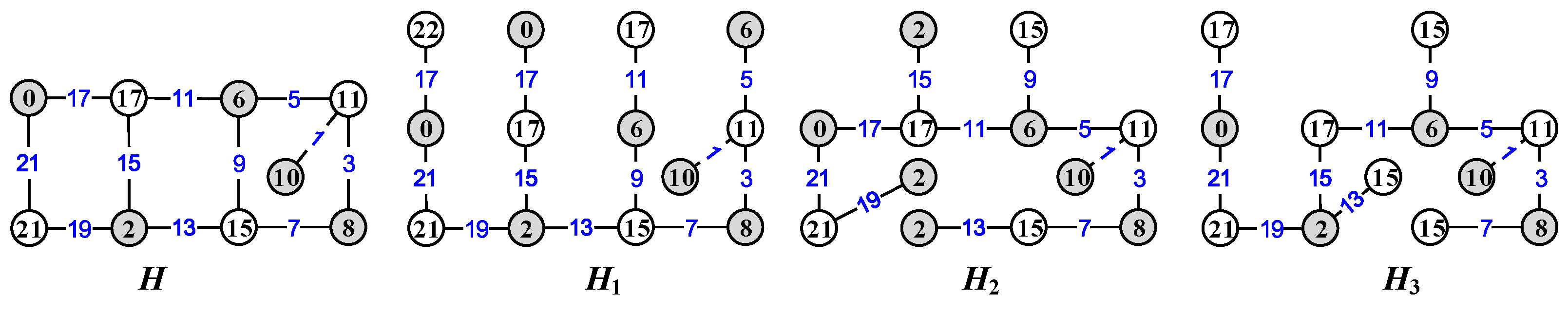
To understand topological graphic passwords, we provide an example as follows: Four colored graphs shown in Figure 1 are topological graphic passwords in topological coding, and they are used as public keys and private keys. The first graph H is a public key, and are private keys, respectively. We obtain a matrix for vertices, edges, and vertices in order, which we call a topological matrix; a topological matrix of order is a graph G with p vertices and q edges, that is
represents a function to obtain the color of vertices and edges. The topological matrix of G can derive number strings, which can be used as digital-based passwords, and preset coloring may be needed during authentication, called topological authentication. We obtain the topological matrix from Figure 1 and then convert it into a many-number-based string as follows:
and so on. In the same way, the topological matrix and number-based string of the other three private keys can be obtained.
We use the multiple constraints of graph colorings and labelings to propose 6C-labeling, 6C-complementary labeling, and its reciprocal-inverse labeling, since they can be applied to building up topological coding. We show some connections between 6C-labeling and other graph labelings/colorings and show graphs admitting twin-type 6C-labelings, as well as the construction of graphs admitting twin-type 6C-labelings and constructing graph classes with new labels to provide a new technology for topological coding. See the examples in Figure 2 and Figure 3.
1.2. Definitions
The standard terminology and notation of graph theory can be found in [12,13]. The following terminology, notation, labelings, particular graphs, and definitions will be used in later discussions:
- A symbol stands for a consecutive set with integers holding ; denotes an odd-set with odd integers with respect to ; is an even-set with even integers .
- The cardinality of a set X is denoted as .
- The number is called the degree of the vertex v, where is the set of neighbors of the vertex v. If . we call the vertex v a leaf.
- G is a -graph having p vertices and q edges.
Definition 1
([13]). Let a connected -graph G with admit a mapping . For each , the labelings are defined as , and we write the vertex color set by and the edge color set as . We have the following restrictions:
- (1)
- ;
- (2)
- , ;
- (3)
- , ;
- (4)
- ;
- (5)
- ;
- (6)
- ;
- (7)
- G is a bipartite graph with the bipartition such that ( for short).
We define: a graceful labeling α satisfying the restriction (1), (2), and (4); a set-ordered graceful labeling α satisfies (1), (2), (4), and (7), simultaneously; an odd-graceful labeling α satisfies the restriction (1), (3), and (5); a set-ordered odd-graceful labeling θ satisfies the restriction (1), (3), (5), and (7); a set-ordered odd-elegant labeling α satisfies the restriction (1), (3), (5), (6), and (7).
Definition 2
([14]). A total labeling for a bipartite -graph G is a bijection holding:
(i) ;
(ii) Each edge corresponding to another edge holds (or );
(iii) Let for , then there exists a constant such that each edge corresponds to another edge holding (or ) true;
(iv) (or , or , or , or is an odd-set, and is an even-set;
(v) (ve-corresponding) each edge corresponds to one vertex w such that , where is a fixed constant, and each vertex z corresponds to one edge such that , except the singularity ;
(vi) (or ) for the bipartition of .
Then, α is called a 6C-labeling of the bipartite -graph G.
Definition 3.
Let -tree G admit a 6C-labeling f and g be a 6C-labeling of -tree H; if they hold, , and with , then f and g are pairwise reciprocal-inverse. The graph obtained by the coinciding of the vertex of G having with the vertex of H having is called a 6C-complementary labeling.
Definition 4.
Let -graph G admit a total labeling and a -graph H admit another total labeling . If and for , then f and g are reciprocal-inverse (or reciprocal complementary) to each other, and H (or G) is an inverse labeling of G (or H).
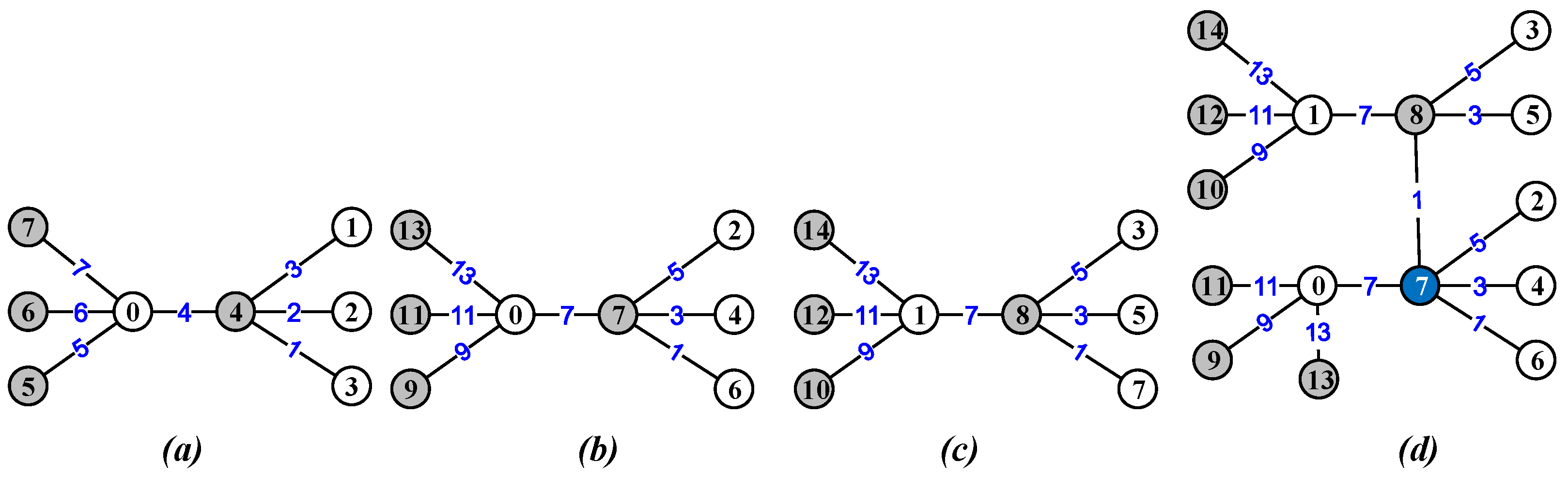
Example 1.
In Figure 3, a tree T admits a 6C-labeling , and other trees admit a 6C-labeling for , where:
(i) for each edge ;
(ii) for each edge ;
(iii) for each edge ;
The graph T and are as defined, then and g are reciprocal-inverse (or reciprocal complementary) to each other, and T (or ) is an inverse labeling of (or T).
Moreover, each 6C-labeling is a reciprocal-inverse labeling of the 6C-labeling , that is and for .
The 6C-labeling and its reciprocal-inverse labeling form a 6C-complimentary labeling for . Each vertex-coinciding tree admits a 6C-complimentary labeling for , where is a self-isomorphic ve-image, since ;
(iv) or with and ;
(v) or with .
If a -graph T has two subgraphs and such that and , we denote T as , called a vertex-identified graph (vi-graph for short). Moreover, we call T a uniformly vertex-identified graph (uniformly vi--graph) if .
Definition 5.
Let a uniformly vi--graph have a mapping f: such that:
(i) for any pair of vertices ;
(ii) f is an odd-graceful labeling (ogl) of ;
(iii) The edge label set . Then, T is called a twin odd-graceful vi--graph, f a twin odd-graceful labeling (togl) of T, a source graph, and an associated graph of .
2. Connections between 6C-Labeling and Other Labelings
Lemma 1.
A -tree T admits a set-ordered graceful labeling if and only if it admits a 6C-labeling.
Proof.
Let and be the bipartition of vertex set of a tree T, where and .
First, notice that is a set-ordered graceful labeling of T, then for and for , and each edge has its label .
Another labeling is defined for the tree T as: for , and
for . The vertex set and edge set is
then we obtain:
(i) .
(ii) Each edge with another edge corresponds and holds such that
(iii) Let for , so
then we obtain a set , where p is even, or a set , where p is odd. Therefore, each edge and another edge correspond, so , except that edge e holds as p is even.
(iv) from Equation (4).
(v) for each edge corresponding to one vertex w, and for each vertex z corresponding to one edge , except the singularity .
(vi) We obtain for the bipartition of .
Therefore, admits a 6C-labeling.
For the converse, let be a 6C-labeling of T. According to the property (iv) and , we obtain the edge label and the vertices’ label set and , respectively. A labeling is defined as: for , which gives ; for each edge , so . The property (i) enables us to compute
that is is graceful. The graceful labeling is set-ordered according to the property (vi). □
Theorem 1.
If two -trees admit set-ordered graceful labelings, then they are a 6C- complementary labeling.
Proof.
Let each tree of p vertices admit a set-ordered graceful labeling and be the bipartition of with . Therefore, we have where and for with . Then, we can label the vertices’ set as for , for and label the edge set as for each edge , and for .
We define another labeling of as: for and for each edge . Therefore, we can compute and .
Next, we define another labeling of as: for each vertex and for each edge . Thereby, we obtain , .
Notice that and . By Lemma 1, we have proven the theorem. □
Theorem 2.
If a -tree T admits a 6C-labeling such that is a 6C-complementary matching, where the tree is a 6C-labeling tree.
Proof.
Let tree T admit a 6C-labeling f, another labeling g of T as for each vertex and for each edge . We obtain with true with . Next, a labeling is defined for a copy of T in this way: for , and for . Notice that
for . We claim that is a 6C-labeling of as well, which means that the proof of Theorem 2 is complete. □
Corollary 1.
Let two trees T and H with p vertices admit set-ordered graceful labelings. Then, admits a 6C-labeling τ with for each edge , and for each edge .
Corollary 2.
Let a tree T admit a set-ordered odd-graceful labeling, then there exists H admitting a twin odd-graceful labeling, where H is a self-corresponding graph.
Proof.
According to the supposition of the corollary, let a tree T have its own vertex bipartition with and with and . For a set-ordered graceful labeling f of T, we obtain for and for , and for each edge :
(1) The labeling is defined for a copy of T with as: for and for ; immediately,
Therefore, is an ogl of , since is an even-set, is an odd-set, and is an odd-set as well. Next, we another another graph obtained by copying T with and make a complementary labeling of the ogl by setting for ; clearly, . Moreover, , ; we can see and . Therefore, is the complementary of . Therefore, admits a togl.
The proof is finished for the corollary. □
Theorem 3.
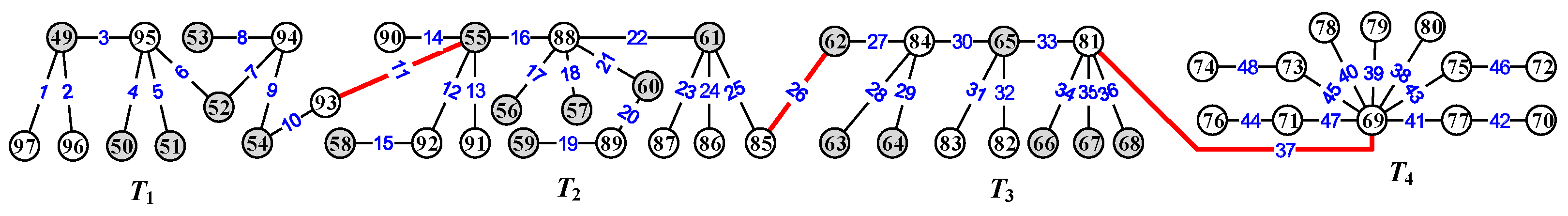
Let be disjoint trees, and each admit a set-ordered graceful labeling for ; is a graceful tree. Then, there are vertices such that joining and for produces a new tree T admitting a 6C-labeling.
Proof.
For each , each tree has vertices and bipartition , where and with .
By the assumption of the theorem, each tree for has a set-ordered graceful coloring holding , , , as well as , which shows that and . has a graceful labeling defined as for and such that and .
We join the vertex with the vertex by an edge, ; we join the vertex with the vertex by an edge, so the resulting tree is denoted as T. Next, we define a labeling g of T in the following steps. Let and , .
We define another labeling g as follows:
Step 1. For each , the vertices’ color of as , , where .
Step 2. The vertices’ color of as , , where .
Step 3. The vertices’ color of as for each , , where .
Step 4. The edges are colored as for , , .
Step 5. The edges are colored as for , .
We can verify the vertices’ and edges’ set as follows:
;
;
;
;
for .
Let us continue to validate the restriction of labeling g as follows:
(i) Each edge :
holds true.
(ii) Each edge corresponding to another edge holds such that
(iii) Let for , so
which distributes a set if p is even or a set if p is odd. Thereby, each edge corresponds to another edge such that , except that edge e holds as p is even.
The proof of (iv)–(vi) is the same as Lemma 1.
Hence, we claim that the labeling f admits really a 6C-labeling defined in Definition 2.
3. Conclusions
This paper studied the 6C-labeling having multiple restrictive conditions and showed the graphic codes. We showed some connections between 6C-labeling and other graph labelings/colorings and showed graphs admitting twin-type 6C-labelings, as well as the construction of graphs admitting twin-type 6C-labelings and constructing graph classes with new labels to provide a new technology for topology coding. The result of Theorem 3 can be used to construct some graphic lattice [15]. If artificial intelligence technology and quantum computer attacks use labels and coloring-generated passwords, the decryption process will involve the determination of the graph isomorphism and some coloring conjectures, so it is not easy to crack. In addition, according to the method proposed in this paper, the topological coding has a variety of graph structures, topological matrices, and number-based strings of topological coding. We can use labeled graphs to design topology coding, so as to ensure information security. We can see that this is easy to obtain from the graph to the matrix and then to the string, and the reverse is difficult. Multiple restrictions also ensure the security of encryption.
Topological graphic passwords are based on the open structural cryptographic platform, that is this platform allows people to make themselves pan-topological graphic passwords by their remembered and favorite knowledge kept firmly in mind. We believe: “If a project has practical and effective applications and is supported by mathematics, it can go farther and farther. Practical application makes it live longer, and mathematics makes it stronger and faster. This project gives people feedback on material enjoyment and returns new objects and problems to mathematics”.
Author Contributions
Data Funding acquisition, C.Y. and S.Z.; Writing—original draft, X.Z. and B.Y.; Writing—review & editing, X.Z. and B.Y.; Supervision, C.Y.and S.Z. All authors have read and agreed to the published version of the manuscript.
Funding
This research was supported by the National Natural Science Foundation of China under Grant No. 61363060 and No. 61662066 and the Science Found of Qinghai Province Grant No. 2021-ZJ-703 and NSFC No. 11661068.
Conflicts of Interest
The authors declare no conflict of interest.
References
- Malutan, R.; Pop, M.; Cislariu, M.; Borda, M. Secure access system on the Q or IQ nxp platform using RSA AND DAS. Acta Tech. Napoc. 2016, 57, 42–45. [Google Scholar]
- Yun, W.X.; Jie, L.M. Survey of Lattice-based Cryptography. J. Cryptologic Res. 2014, 1, 13–27. [Google Scholar]
- Regev, O. On Lattices, Learning with Errors, Random Linear Codes, and Cryptography. J. ACM 2009, 56, 1–40. [Google Scholar] [CrossRef]
- Micciancio, D.; Regev, O. Lattice-based cryptography. In Post-Quanturn Cryptography; Bernstein, D.J., Buchmann, J., Dahmen, E., Eds.; Springer: Berlin/Heidelberg, Germany, 2009; pp. 147–191. [Google Scholar]
- Wang, H.; Xu, J.; Yao, B. Twin Odd-Graceful Trees Towards Information Security. Procedia Comput. Sci. 2017, 107, 15–20. [Google Scholar] [CrossRef]
- Anuj, K.; Amit, K.V. Application of graph labeling in crystallography. Mater. Today Proc. 2020, in press. [Google Scholar] [CrossRef]
- Ascher, E. Aloysio Janner Algebraic aspects of crystallography. Commun. Math. Phys. 1968, 11, 138–167. [Google Scholar] [CrossRef]
- Tian, Y.; Li, L.; Peng, H.; Yang, Y. Achieving flatness: Graph labeling can generate graphical honeywords. Comput. Secur. 2021, 104, 102212. [Google Scholar] [CrossRef]
- Mageshwaran, K.; Kalaimurugan, G.; Hammachukiattikul, B.; Govindan, V.; Cangul, I.N. On-Labeling Index of Inverse Graphs Associated with Finite Cyclic Groups. J. Math. 2021, 2021, 5583433. [Google Scholar] [CrossRef]
- Prasanna, N.L.; Sravanthi, K.; Sudhakar, N. Applications of Graph Labeling in Communication Networks. Orient. J. Comput. Sci. Technol. 2014, 7, 139–145. [Google Scholar]
- Balakrishnan, R.; Ranganathan, K. A Textbook of Graph Theory; Springer: Berlin/Heidelberg, Germany, 2008. [Google Scholar]
- Bondy, J.A.; Murty, U.S.R. Graph Theory; Springer: London, UK, 2008. [Google Scholar]
- Gallian, J.A. A Dynamic Survey of Graph Labeling. The Electronic Journal of Combinatorics. 2021. DS61. Available online: https://www.combinatorics.org/ds6 (accessed on 13 March 2022).
- Yao, B.; Sun, H.; Zhang, X.; Mu, Y.; Sun, Y.; Wang, H.; Su, J.; Zhang, M.; Yang, S.; Yang, C. Topological Graphic Passwords And Their Matchings Towards Cryptography. arXiv 2018, arXiv:1808.03324v1. [Google Scholar]
- Su, J.; Sun, H.; Yao, B. Odd-Graceful Total Colorings for Constructing Graphic Lattice. Mathematics 2022, 10, 109. [Google Scholar] [CrossRef]
Figure 1.
A set-ordered odd-graceful topological public key H and its own topological private keys .
Figure 1.
A set-ordered odd-graceful topological public key H and its own topological private keys .

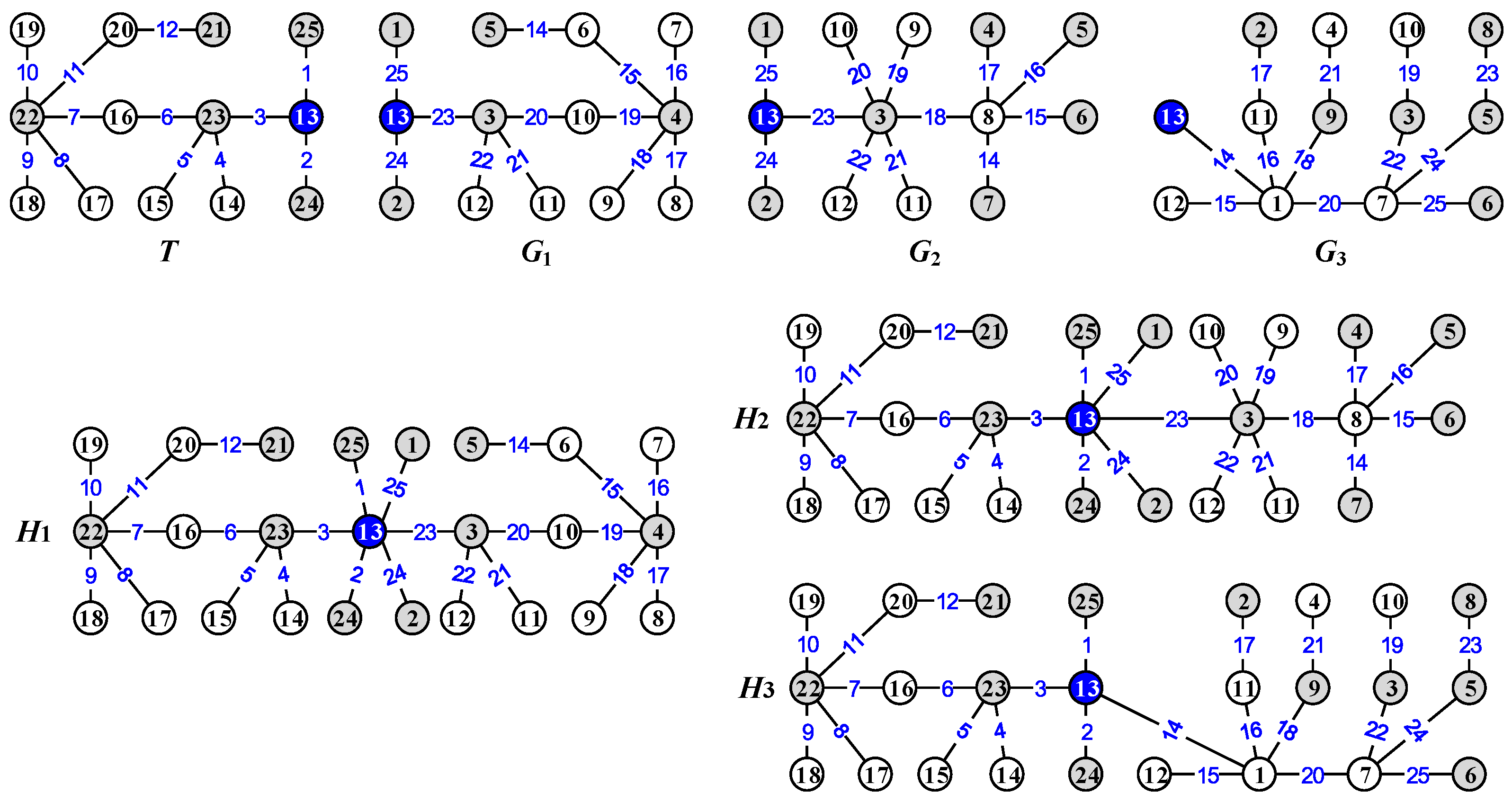
Figure 2.
Examples The graphs for illustrating the 6C-labeling defined in Definition 2, the graphs reciprocal-inverse labeling defined in Definition 3, and the 6C-complimentary matching defined in Definition 4.
Figure 2.
Examples The graphs for illustrating the 6C-labeling defined in Definition 2, the graphs reciprocal-inverse labeling defined in Definition 3, and the 6C-complimentary matching defined in Definition 4.

Figure 3.
Examples for illustrating Corollary 2. (a–d) are T, , , and , respectively.

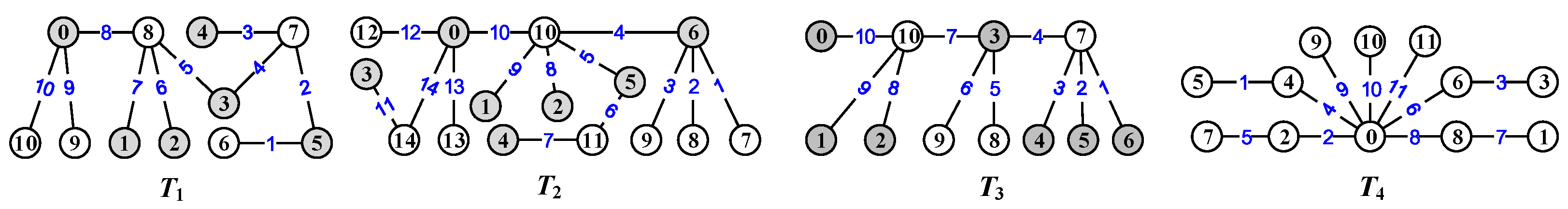
Figure 4.
Four graphs with for understanding the proof of Theorem 3.

Figure 5.
An example for illustrating the proof of Theorem 3.

Publisher’s Note: MDPI stays neutral with regard to jurisdictional claims in published maps and institutional affiliations. |
© 2022 by the authors. Licensee MDPI, Basel, Switzerland. This article is an open access article distributed under the terms and conditions of the Creative Commons Attribution (CC BY) license (https://creativecommons.org/licenses/by/4.0/).
Share and Cite
MDPI and ACS Style
Zhang, X.; Ye, C.; Zhang, S.; Yao, B. Graph Colorings and Labelings Having Multiple Restrictive Conditions in Topological Coding. Mathematics 2022, 10, 1592. https://doi.org/10.3390/math10091592
AMA Style
Zhang X, Ye C, Zhang S, Yao B. Graph Colorings and Labelings Having Multiple Restrictive Conditions in Topological Coding. Mathematics. 2022; 10(9):1592. https://doi.org/10.3390/math10091592
Chicago/Turabian StyleZhang, Xiaohui, Chengfu Ye, Shumin Zhang, and Bing Yao. 2022. "Graph Colorings and Labelings Having Multiple Restrictive Conditions in Topological Coding" Mathematics 10, no. 9: 1592. https://doi.org/10.3390/math10091592
Note that from the first issue of 2016, this journal uses article numbers instead of page numbers. See further details here.