
A Novel Low-Query-Budget Active Learner with Pseudo-Labels for Imbalanced Data


Center for Applied Data Science Gütersloh (CfADS), FH Bielefeld-University of Applied Sciences, 33619 Bielefeld, Germany
*
Author to whom correspondence should be addressed.
Mathematics 2022, 10(7), 1068; https://doi.org/10.3390/math10071068
Submission received: 31 January 2022
/
Revised: 18 March 2022
/
Accepted: 23 March 2022
/
Published: 26 March 2022
(This article belongs to the Special Issue Machine Learning for Technical Systems)
Abstract
:Despite the availability of a large amount of free unlabeled data, collecting sufficient training data for supervised learning models is challenging due to the time and cost involved in the labeling process. The active learning technique we present here provides a solution by querying a small but highly informative set of unlabeled data. It ensures high generalizability across space, improving classification performance with test data that we have never seen before. Most active learners query either the most informative or the most representative data to annotate them. These two criteria are combined in the proposed algorithm by using two phases: exploration and exploitation phases. The former aims to explore the instance space by visiting new regions at each iteration. The second phase attempts to select highly informative points in uncertain regions. Without any predefined knowledge, such as initial training data, these two phases improve the search strategy of the proposed algorithm so that it can explore the minority class space with imbalanced data using a small query budget. Further, some pseudo-labeled points geometrically located in trusted explored regions around the new labeled points are added to the training data, but with lower weights than the original labeled points. These pseudo-labeled points play several roles in our model, such as (i) increasing the size of the training data and (ii) decreasing the size of the version space by reducing the number of hypotheses that are consistent with the training data. Experiments on synthetic and real datasets with different imbalance ratios and dimensions show that the proposed algorithm has significant advantages over various well-known active learners.
1. Introduction
Due to the massive number of IoT devices (e.g., monitoring components and sensors) and seemingly endless Internet data (e.g., images, videos, sound signals, and texts), the amount of free unlabeled data is enormous, and due to the cost of the labeling process, annotating these data or even a suitable portion of them to create sufficient training data for developing machine learning applications has become a new challenge for data scientists [1,2]. This is because the labeling process is (i) time-consuming when, for example, the expert must label long documents, (ii) expensive because experts with extra facilities (e.g., laboratories) might be needed, or (iii) difficult because the numbers of data in some classes are limited in many applications—e.g., faulty classes in industrial applications. The active learning technique provides a solution by reducing the size of the training data and annotating only the most informative points to obtain high-quality training data [3,4,5].
In an active learning technique, given unlabeled data, a specific query strategy is used to select one or many points and query them. Increasing the number of queries (i.e., query budget), which is always limited, expands the explored area in the search space, which improves the overall classification performance [6,7,8]. However, due to the high cost of the labeling process, the main goal of active learners is to cover the most informative parts within the instance space with the fewest labeled points (low query budget), which enables better generalization.
Active learning algorithms can operate in three different scenarios. The first scenario is the membership query synthesis active learning scenario. Here, the learner generates a synthetic/artificial point in the input space and then requests a label for it. Since these points are generated synthetically, some of them could not be labeled in a reasonable way [9,10]. The second is the stream-based selective sampling scenario, where the learning algorithm decides whether to label each unlabeled data point based on its information [11,12]. This approach is also called sequential active learning, since each unlabeled point is drawn sequentially. Third, the pool-based sampling scenario is the most well-known scenario. In this scenario, the trained active learner is used to evaluate and then select some instances from the large set/pool of unlabeled data. Depending on the informational content of these instances, queries are selectively drawn from the pool [10,13].
The query strategy in many active learners searches for the most informative points that are expected to be around the decision boundaries between classes as in [14,15], whereas the other active learning strategies search for the most representative points to cover the entire data distribution as in [16,17]. In the proposed algorithm, we try to combine both search strategies to query the most informative and the most representative points. Moreover, most of the current active learners need initial knowledge, such as initial training data (labeled points), the number of classes, and an indication of which are the minority and the majority classes when the data are imbalanced. However, preparing initial training data, especially with imbalanced data, increases the labeling cost and may be not possible in some real scenarios. In addition, the number of classes might change. Therefore, there is a need for an active learner that does not require predefined knowledge (i.e., it could adapt itself with the new data), even for real-world challenges such as the imbalanced data problem, which is one of the goals of our proposed active learner. This flexible strategy allows our model to cover a large area in the space to find the minority classes (if any).
Inspired by the active learning model in [10], with the aim of selecting high-quality labeled data that could partially cover the minority class subspace in a case of imbalanced data, and without any predefined knowledge, the proposed low-query-budget active learner (LQBAL) combines the advantages of selecting both informative and representative points by using two phases. The first one is the exploration phase, where the search space is well covered by iteratively exploring new regions. This could be done by iteratively searching for the least explored regions within the space and exploring them by annotating the most representative points there. The second phase is the exploitation phase, which aims to select the most informative points by annotating representative points within the uncertain, critical, or disagreement regions between different trained learning models. Since (i) very small changes in inputs do not lead to large changes in outputs [18], and (ii) the query budget is always low due to the high labeling cost, the proposed algorithm increases the supervised knowledge by iteratively adding some pseudo-labeled points that lie around the new labeled points. The main contributions of this work are as follows:
- A novel active learner with a low query budget and pseudo-labeled data is proposed to deal with imbalanced data. Our novel strategy for finding the most informative and the most representative points increases the probability of selecting instances from the minority class, which is challenging with high imbalance ratios. Further, the proposed model can adapt to different variations of the received data (e.g., balanced data, imbalanced data, binary classes, or multi-class) without any predefined knowledge.
- We propose a method to enrich the supervised knowledge that our active learner collects by adding some pseudo-labeled points (PLs) that are geometrically close to the new labeled points. Further, our model assigns weights to the generated PLs based on the density of labeled points around each pseudo-labeled point. In addition to increasing the supervised knowledge, the pseudo-labeled points play a role in reducing the version space in one of the pruning steps, minimizing the size of uncertain regions. This encourages our algorithm to focus on the most uncertain parts of the space, which could help to find highly informative points. In addition, searching for conflicting pseudo-labeled points (points that are near two or more annotated points that belong to different classes) guides our model to accurately find uncertain regions between different classes.
- A part of the proposed algorithm builds a novel, flexible learner that learns from training data points (annotated points by experts + PLs) with different confidence values.
To evaluate the proposed model, we conducted a set of experiments with imbalanced data. In the first experiment, synthetic data containing linearly separable, non-linearly separable, balanced, and imbalanced classes were used. The performance of the proposed algorithm was also tested against real imbalanced datasets with low and high imbalance ratios. In those experiments, we used a set of real imbalanced datasets with multiple classes for testing how our model covers minority classes in multi-class scenarios.
The rest of the paper is organized as follows: Section 2 introduces the theoretical background of active learning techniques, an illustrative example to compare between querying instances randomly and using an active learner, and finally some of the work related to the active learning technique. The algorithmic steps of the proposed model are explained in Section 3. Section 4 presents a set of experiments to compare the proposed model with different state-of-the-art active learning techniques using different experimental scenarios. Finally, concluding remarks and future work are provided in Section 5.
2. Theoretical Background
There are two main types of machine learning algorithms: supervised and unsupervised. The supervised ones need training/labeled data to learn. These training data consist of a set of labeled instances (), where is the labeled data, is the number of labeled data points, is one point, d is the number of attributes/features (i.e., the dimensionality of the feature space), and denotes the label for each instance (), where , is the ith class, and C is the number of classes. In the unsupervised algorithms, the data are structured as follows: , where is the unlabeled data and is the number of unlabeled instances.
Since collecting real data is expensive and time-consuming, it is a big challenge to train supervised learning models using fully labeled data. The partially-supervised machine learning approach offers an alternative by using both the labeled and unlabeled data (). This approach has two main techniques: The first is the semi-supervised technique, which uses the unlabeled data for further improvement and constrains supervised learning models that learned from the labeled data [19]. The second technique is the active learning technique, which has an additional query component that evaluates the informativeness of the available unlabeled points to select the most promising ones from the set of unlabeled data for annotation [20,21].
Figure 1 shows how an active learner works. All unlabeled points are grayed out. Based on a specific query strategy, some unlabeled points will be selected to be queried by one or more experts. A learning algorithm trained with the current labeled points is employed for selecting some points (the two yellow points) for querying them. These selected points are annotated by an expert and then added to the labeled data. Iteratively, the current labeled points will be used to re-train the learning model to improve it. Finally, the outputs of the active learner are a set of labeled points and a model trained on this labeled set.
2.1. Illustrative Example
The goal of this example is to show how the classification accuracy is affected by the selected labeled points. In this example, we compare the random selection and the selection using a simple active learner. We used the Iris dataset, one of the most well-known classification datasets, which consists of three classes of 50 points each, and each point is represented by four features. In our example, we used only two features for the purpose of visualization, and to simplify the example, we used only two classes. Figure 2a shows the original data points from both classes. As shown, there is an overlap between the two classes. Initially, all points in each run were considered unlabeled. These points are represented by filled black circles in Figure 2b. From the total number of points, 10% were randomly selected as training data by making their labels available. In the figure, these training data points are represented by black dots each surrounded by a blue or red circle. Iteratively, each selection method (i.e., random or active learner) selected a point to label, and this new labeled point was then added to the training set for retraining the model. In this example, the active learner was very simple: it trained a Naive Bayes classifier with the training set, and the trained model was then used to predict the posterior probability of the remaining data. For example, given two classes, the posterior probabilities of a point are ; therefore, the probability that belongs to the first (second) class is 0.9885 (0.0115). In our example, the Naive Bayes classifier was chosen because of its simplicity, but also because it belongs to the "probabilistic classification" family, which provides a probability distribution over a set of classes. Based on the predicted posterior probabilities (i.e., the outputs of the Naive Bayes classifier), the least confident method [19] was used to query a new point. As shown, the random sampling method selected the points pure randomly, while the active learner selected the points on the boundaries between the two classes. The accuracy results of this simple experiment are illustrated in Figure 2c. It can be seen that the active learner’s selection of the labeled points improved the accuracy much better than the random selection. Further, in contrast to the active learner method, the large error bars of accuracy for the random selection show that this method is not stable.
Using this illustrative example, it is clear that the active learner improves its classification performance iteratively by querying the most informative instances and adding them to the training set to further train the classifier.
2.2. Active Learning with Imbalanced Data: State-of-the-Art
The performances of passive and active learning models are highly affected by the presence of imbalanced data [22]. This is because, in some cases, the model cannot learn efficiently from the minority class in the presence of passive learners, especially when the imbalance ratio (IR: the ratio between the number of majority class points and the number of minority class points) is high (i.e., the minority class is very small compared to the majority one). This deteriorates the classification results of minority classes. Additionally, a small training dataset may reduce the chance of learning from the minority class. In the active learning technique, the chance of annotating a minority point is small compared to finding a majority point. However, many active learners, such as those in [23,24,25,26,27], select instances without considering the class distribution. The classical resampling techniques, such as the random undersampling and random oversampling techniques, have been employed for solving the imbalanced data problem with active learners. For example, in [28], the minority data points from earlier batches were propagated, while the majority data points of the current batch were undersampled. In [29], only the minority points that were similar to the current batch were oversampled. The Learn++.CDS algorithm used the synthetic minority over-sampling technique (SMOTE) algorithm for balancing the data [30]. In another study, an active learner that prioritized the labeling of minority class observations was introduced in [31] to improve the balance of the learning process. Recently, in [32], a new active learner method was introduced for multiple classes imbalanced data. In [10], a novel strategy was introduced to find the most informative and the most representative points with the aim of increasing the chance of finding and covering the minority class.
In general, most active learning models that are already designed to handle imbalanced data should first be informed about which class is the minority one. Additionally, these active learning models need to be initialized with some labeled points from the minority class. (For example, the authors of [33] supposed that they had initially an opposite pair: one point from each class, in the case of binary classes). This is challenging and may be impractical in many environments. This is because, for example, new classes of faults may appear in industrial applications. This motivated us to present a novel active learner that can adapt to newly received data without any predefined knowledge.
3. The Proposed Model
In our model, we assume that all the available data points are unlabeled, and this set is represented as follows: , where is an unlabeled instance/point. This is the worst-case scenario (i.e., there is no initial training or labeled data), and this could be the case, for example, at the beginning of the installation of active learners. However, our model could also handle partially labeled data (see Section 4.3). In our model, the query budget is denoted by Q. Mathematically, the labeled data are denoted by , and the number of labeled points is denoted by . Moreover, initially, there is no predefined knowledge about the number of classes and the presence of imbalanced data. In our model, the lower and upper limits of the ith-dimension in the space are denoted by and , respectively, and the corresponding vectors are and .
As mentioned earlier, in the proposed model, we aim to annotate only a few instances due to the high cost of the annotation process, which is why we called our model the low-query-budget active learner (LQBAL). Our model starts by annotating the first point (see Section 3.1). After that, the model uses one of two phases (exploration and exploitation phases) to query a new point. In the exploration phase, our model attempts to explore new regions by searching for the least explored regions and annotating representative points there. While in the exploitation phase, our model aims to use the knowledge extracted from the first phase and query points in uncertain, critical, or disagreement regions that are believed to be at the decision boundaries between different classes. To select the most informative and representative points, a balance should be established between the two phases. This balance is established by the parameter a, which is used for switching between the two phases as follows:
where is a random number and a is called the exploration-exploitation parameter, which is iteratively decreased smoothly from one to zero throughout the course of learning as follows:
where Q is the query budget and is the number of labeled data points. The above equation means that the proposed model tends to explore (i.e., use the exploration phase) the space at the beginning; that after some iterations, the model might use one of the two phases; and finally, that in the last iterations, the model will use the exploitation phase. Since the exploitation phase requires labeled data for training learning models, our model will only use this phase if the currently labeled points by the exploration phase belong to different classes, not just one class.
In our model, first, the search space will be divided into different parts or cells. In accordance with Latin hypercube (LHC) sampling method [34,35], where the dimensions of the space are divided into equal intervals and a point is randomly generated within each interval, we first divide each dimension of the input space into equal intervals ( is the number of subdivisions in each dimension). Hence, selecting a large increases the number of cells; consequently, increases the required computational cost (more details on the computational analysis of our model are in Section 3.6). Therefore, in our model, to avoid a high computational cost, each dimension within the space is divided into only divisions. For example, with three-dimensional space (i.e., ), the space is divided into cells. The cells are denoted by , where k is the number of cells. In our model, in both phases, only one cell will be selected to be explored by annotating one point within its borders. To avoid selecting a cell multiple times, the selected cell containing the new annotated point is further subdivided into smaller cells. This prevents our model from examining the same cell many times; instead, the model focuses on smaller parts within that cell that may contain more information than the others.
With the aim of increasing the supervised knowledge without additional labeling cost, in the proposed model, we use some additional pseudo-labeled points (more details in Section 3.4). The steps of the proposed model are illustrated in Algorithm 1, and Table 1 lists the notation and their descriptions used in this paper.
| Algorithm 1 Annotate a set of unlabeled points. = LQBAL (). | ||
| Input: Unlabeled data () and Q | ||
| Output: Labeled points () | ||
| 1: | Calculate , , , and d | |
| 2: | Divide the space into equal cells, , where k is the number of cells | |
| 3: | Set , , , , and | |
| 4: | QueryingFirstPoint () | |
| 5: | for to Q do | |
| 6: | ||
| 7: | if then | ▹Exploitation phase |
| 8: | Exploitationphase () | |
| 9: | else | ▹ Exploration phase |
| 10: | ExplorationPhase () | |
| 11: | ||
| 12: | ||
| 13: | , | ▹ select the nearest unlabeled |
| points to to be pseudo-labeled points | ||
3.1. Querying the First Point
In many modern active learners, the initial points are randomly selected and annotated [10]. This may result in selecting one of the outliers or a point that does not contain representative or discriminatory information that helps with exploring the search space. In our model, we instead select the point closest to the mean of the unlabeled data after ignoring (but not removing) the outliers (see Figure 3). The outlier points in this step have more than 1.5 interquartile ranges above the upper quartile or below the lower quartile, and this method is useful when the data are not normally distributed. The first selected point () is then annotated and added to the labeled data as follows: , and then deleted from the unlabeled instances (). However, with imbalanced data, it is very likely that the outliers could represent some/all minority points. Therefore, removing the outliers increases the probability that the first point belongs to the majority class. This means that in the early stages of active learning, when the model does not yet have enough knowledge (somewhat naively), the minority class can be completely missed if active learning scans the problem space for hard-to-find but critical minority points; this agrees with [36]. However, with/without considering the outliers, the probability that the first selected point belongs to the majority class is higher than the probability that it belongs to the minority class, and this probability is proportional to the imbalance ratio; and even with the most advanced active learning methods, there is no guarantee that the first point belongs to the minority class, especially when the method has no predefined knowledge, which is the case for our proposed model.
As we mentioned before, after selecting and annotating a new point, the cell containing this new annotated point will be further subdivided in the same way (i.e., each dimension of the cell is divided into intervals) and the original cell will be deleted. Figure 3 explains how the two-dimensional space is divided into four cells and the cell containing the new annotated point (the red point) is further subdivided into smaller ones.
Repeatedly dividing cells into smaller ones increases the number of cells, which increases the computational complexity of our model. For example, with , the space would be divided into cells, and with each new annotated point, one cell would be further subdivided into new 1024 cells. Thus, after annotating 10 points, the total number of cells would be 11,254. However, many of these cells do not have data points (e.g., the two highlighted cells in the lower-left corner in Figure 3); therefore, our model removes these cells to reduce the overall complexity of the computation. The steps of querying the first point are illustrated in Algorithm 2.
| Algorithm 2 Annotating the first point. QueryingFirstPoint (). | ||
| Input: | ||
| Output: The first labeled point (), | ||
| 1: | , | ▹ is the outliers of |
| 2: | ▹ is the mean of | |
| 3: | ||
| 4: | ||
| 5: | ||
| 6: | , | ▹ select the nearest unlabeled points |
| to to be pseudo-labeled points, all of them belong to the class of | ||
| 7: | for to k do | |
| 8: | if within the borders of then | |
| 9: | Divide into cells and delete | |
| 10: | Delete all cells that have no data | |
3.2. Exploration Phase
The goal here is to annotate new points in regions we have not yet visited or explored by searching for the most informative and the least explored region and exploring it (the region) by annotating one representative point there. This could be achieved in our model, iteratively, by counting the number of labeled and unlabeled points within the borders of each cell. After that, the cell that has the maximum ratio between the number of unlabeled points and the number of labeled points (since the number of labeled points in some cells is expected to be zero, in our model, we calculate the ratio of the number of unlabeled points to the number of labeled points ) will be selected for exploration. This high ratio of a cell indicates that this cell has many unlabeled points (highly informative) and a low number of labeled points (low exploration power); hence, this cell is still uncertain even if it has been explored before by annotating some labeled points within its borders. Therefore, for further exploring this cell, a new point within its boundaries must be annotated.
After selecting the cell to be explored, the easiest way to annotate a new point is to randomly annotate an unlabeled point. However, the selected point could be (i) near one of the currently labeled points in the same cell or the neighboring cells, so the new annotated point may be redundant/duplicative or (ii) an outlier within the cell. Therefore, if the cell has one or more labeled points, among the unlabeled points within the borders of the selected cell, the model will select the farthest point from the labeled ones (to explore a new region); otherwise, the model will select the nearest point to the center of the unlabeled data points within this cell (to select the most representative point). The steps of the exploration phase are illustrated in Algorithm 3.
3.3. Exploitation Phase
After labeling some points in the exploration phase, the model might use the exploitation phase with the aim of annotating new points within uncertain region(s) that are expected to be around the decision boundaries between classes. This phase starts by training different hypotheses given the current annotated points. Different steps are then taken for pruning these hypotheses and keeping the most accurate and diverse ones. Next, the most disagreement/critical region between the remaining hypotheses is determined. To explore this region, one point within its boundaries will be queried. The steps of this phase are explained in the following sections.
3.3.1. Generating/Training Classifiers
Given a set of labeled points from the exploration phase (), the aim of this step is to generate a set of hypotheses/classifiers/weak learners () that are trained using , where is the ith hypothesis in the tth iteration, the weak learners are simple classifiers that always perform poorly (better than chance or slightly better than 50% accuracy) when trying to label the data [37], and m is the number of new trained hypotheses in each iteration. We thought of using weak learners due ensemble learning methods. We hypothesized that a strong learner could be constructed by combining many weak learners [38]. In our model, we use the multilayer perceptron (MLP) classifier [39,40]. The MLP iteratively increases the number of hypotheses. For example, after 20 iterations, since each generates 100 new hypotheses (i.e., ), the total number of generated hypotheses will be 2000. However, increasing the number of hypotheses increases the chance of getting diverse hypotheses, and precisely determines the critical region. However, this large number of hypotheses increases the required computational cost, which may reduce the applicability of our model. Moreover, since the hypotheses are generated iteratively, not all of them are consistent with the new labeled points. As a consequence, some of these hypotheses should be pruned to reduce the number of hypotheses and keep only the most accurate ones (i.e., consistent with the training data).
| Algorithm 3 Querying a new point using the exploration phase. = ExplorationPhase (). | ||
| Input: | ||
| Output: New labeled point and | ||
| 1: | for do | |
| 2: | for do | |
| 3: | if is within the borders of the cell then | |
| 4: | ▹ : the number of labeled points within the cell | |
| 5: | for do | |
| 6: | for do | |
| 7: | if is within the borders of the cell then | |
| 8: | ▹: the number of unlabeled points | |
| within the cell | ||
| 9: | ▹ the selected cell | |
| 10: | if then | ▹ if the cell has labeled points |
| 11: | is farthest unlabeled point from the labeled ones within the cell | |
| 12: | else | |
| 13: | is the nearest unlabeled point to the center of the unlabeled points within the cell | |
| 14: | Query () | |
| 15: | Divide into cells and delete | |
| 16: | Delete all cells that have no data | |
3.3.2. Classifier Pruning
Decreasing the number of trained hypotheses by selecting the best ones minimizes the version space, which is the set of hypotheses that are consistent with the training data (i.e., the hypotheses that classify the training/labeled patterns correctly). This decreases the overall computational time and also minimizes the uncertain regions, which provides the opportunity to focus on the most uncertain parts within the space. Therefore, our model has three different pruning steps.
The first pruning step aims to prune the new trained hypotheses. This could be done by selecting the best hypotheses from the trained ones. The selected set has the most consistent ones with the current labeled data points, and it is denoted by , where t is the current iteration. To select only the most consistent hypotheses with the current training data (i.e., labeled points), the proposed model checks whether the current training data are imbalanced, and with balanced (imbalanced) training data the hypotheses are sorted according to their accuracy (Geometric Mean (GM) [41]) results, where GM , is the true positive rate, is the true negative rate, represents true positives, is true negatives, is the false positives, and indicates false negatives [41]. After sorting the new trained hypotheses according to their results, the hypotheses that obtained accuracy/GM results above 50% will be selected; these hypotheses represent the weak learners in our model, and 50% was chosen as a threshold to ensure that each hypothesis correctly classified at least 50% of the data points [37,42]. These selected hypotheses are denoted by , where is the ith selected hypothesis in the tth iteration and is the number of selected hypotheses. The selected hypotheses () will be added to the final set of hypotheses that were collected in the previous iterations. The final set of hypotheses is denoted by , where is the number hypotheses in .
For example, assume that we have six generated hypotheses , the labeled data points are balanced, and the accuracies of these hypotheses are 55%, 78%, 60%, 50%, 80%, and 90%, respectively. After sorting the hypotheses according to their accuracies, the selected hypotheses will be .
Since the final hypotheses () set always contains hypotheses from previous iterations, some of these hypotheses might be not consistent with the new annotated points, which reduces the classification performance of these hypotheses. As a result, these hypotheses that have poor performances should be iteratively deleted. Therefore, the second pruning step is to iteratively remove all hypotheses from that are not consistent with the current labeled points.
Logically, the critical region includes regions with different uncertainties because the borders of the critical region are determined by some hypotheses that might be affected by tuning their parameters. Therefore, small changes in some of these hypotheses might change the borders of the critical region. This means that the centers of the critical regions always have uncertainties higher than the uncertainties in the regions near the borders of the critical region. Thus, with the aim of shrinking the critical region, in the third pruning step, to get the final set of hypotheses, our model keeps only the hypotheses that are consistent with current labeled data and the pseudo-labeled points (for more details about the pseudo-labeled points, see Section 3.4). The final set of hypotheses after this third pruning step represents the final version space.
Figure 4 illustrates (i) the hypotheses (in the first row), (ii) a simulation of the version space (in the second row), which is bounded by the consistent hypotheses (the highlighted area with the green color in the second row), and (iii) the uncertain region in the instance space, which is bounded by the current hypotheses (gray area in the third row).
- The first column shows the final hypotheses in the last iteration (i.e., ), of which there were five; all of them are consistent with the two labeled points (the labeled points from the previous iterations). As shown, the uncertain region (third column) is very wide, and some hypotheses might be redundant (i.e., they are not used for constructing the uncertain region). Moreover, the version space (second column) is also wide, and it is bounded by the most general hypothesis () and the most specific one ().
- After annotating a new point, some new hypotheses will be trained on the current labeled points (the two old labeled points and the new one). From the newly generated hypotheses, the first pruning step (in the second column in the figure) keeps only the consistent hypotheses with the current labeled points. As shown, after the first pruning step, there were only six remaining new hypotheses in green color, and the inconsistent ones are the two in gray. The second row shows how the first pruning step (second column) removes directly the new hypotheses that are not consistent with the data, which reduces the version space; the red part in the figure represents the deleted part of the version space after applying the first pruning step. Further, labeling new points helps to explore new regions within the space, reducing the uncertain region, as in the third row.
- In the third column and first row in the figure, these remaining new hypotheses (the green ones in the second column) are added to the selected hypotheses from the previous iterations () (the dashed black ones in the first column), which increases the number of hypotheses. As illustrated, not all hypotheses are consistent with the new labeled point, such as the hypothesis that is represented by a dashed gray line. In the second pruning step, this hypothesis was removed.
- Finally, the fourth column in the figure shows how the pseudo-labeled points might help to shrink the version space by removing some hypotheses from that are not consistent with them. As shown, in the first row, the gray lines represent the hypotheses in that are not consistent with the pseudo-labeled points. These were removed, and only three hypotheses were kept after applying the third pruning step, which reduced the version space (in the second row) and the uncertain region (in the third row).
It is worth mentioning that the motivation for keeping hypotheses from the previous iterations is to create a diverse set of hypotheses. As shown in the figure, adding hypotheses from to the final set of the selected hypotheses () reduces the version space slightly and adds diverse hypotheses. Hence, iteratively annotating some points using the exploitation phase reduces the version space, decreases the size of the uncertain region, and approximates the decision boundaries between different classes increasingly accurately.
In our model, during the exploration phase, all hypotheses in were kept, and all the new annotated points were used for pruning the hypotheses in in the next exploitation iteration.
3.3.3. Determining the Critical Region
The critical or uncertain regions are those with the highest scores of disagreement between hypotheses in . The goal of the proposed model is to explore this region by annotating one point that shrinks the version space. This is similar to the support vector machine (SVM) classifier, where the decision boundary is usually in the middle of the version space, and adding a new point near this decision boundary roughly splits the version space in half [26]. This is also illustrated in the example in Figure 4: adding a new annotated point shrinks the version space, which also reduces the uncertain region.
Mathematically, the critical region between only two hypotheses () is formally defined as follows:
where p is a point in the space and is the critical region in the iteration t. The disagreement or uncertainty score () is calculated using many methods, and one of the most well-known is the vote entropy method, which is defined as follows:
where indicates all possible labels, is the number of hypotheses in , and is the number of votes that a label receives from the prediction of the hypotheses. For example, take three classes (i.e., ) and with 12 classifiers (i.e., ). The take two instances, and . For , let the votes be as follows: , , and . Hence, the vote entropy of is . For , let ; thus, it is difficult to determine the class label of , and the vote entropy is . Hence, the level of disagreement of is higher than ; as a result, will be queried (i.e., ).
Scanning the whole space to find uncertain regions (the regions with high USs) is computationally expensive, especially with high-dimensional datasets. Further, some parts within the space might have not data points. Scanning these parts, therefore, would waste many calculations for nothing. Therefore, the proposed model calculates the disagreement score for only the unlabeled data points. After that, the disagreement score (or uncertainty score) for each cell is calculated by summing the scores of the unlabeled points within its borders (), where is the uncertainty score of the cell . The cell that has the maximum uncertainty score will be selected for exploring it by annotating the (i) most uncertain point within that cell and (ii) the farthest point from the labeled data within that cell (if any).
During our initial experiments, it is worth noting that the search strategies of the exploration and exploitation phases always helped to query points in new regions or the most uncertain ones. This increased our chances of querying points from minority classes, even with a low query budget.
3.4. Adding Pseudo-Labeled Points
To increase the supervised knowledge without additional labeling cost, we used some additional pseudo-labeled points (PLs) to increase the amount of training data (i.e., training data = labeled data () + pseudo-labeled points ()). The new PLs were meant to help the learning models to generalize better by moving the decision boundaries to low-density regions between classes. The classical methods for selecting PLs start by training a learning model with the available training or labeled data. Then, the labels of the unlabeled data are predicted and the most reliable PLs are added to the original training data. These new training data are used to retrain the learning model. However, without sufficient labeled points that capture the structure of the data, the trained model might be poorly calibrated, resulting in incorrect pseudo-labeling (i.e., noisy pseudo-labels) and poor generalization. In other words, the accuracy of PLs depends on the initial predictions, which requires a sufficient number of initial labeled points. Figure 5 shows the well-known example from [43], where the two-moons dataset (we used the code in https://uk.mathworks.com/matlabcentral/fileexchange/41459-6-functions-for-generating-artificial-datasets (accessed on 28 January 2022) to generate 1000 points of the two-moons dataset) was generated and initially only three points from each class were labeled. The figure shows that the trained models using only a few labeled points correctly classified the labeled set, but certainly they will have high test error rates because these models deviate greatly from the true target function. Consequently, these trained models are expected to produce noisy PLs. In addition, the main disadvantage of these classical methods is that they are not able to correct their own errors, resulting in a larger number of erroneous pseudo-labels. These limitations of the classical methods for generating PLs, and the goal of using only a low query budget, motivated us to have our model search geometrically in the unlabeled data for the PLs that are near to the newly annotated points. One of the main advantages of our strategy is that it does not require any predefined knowledge. Further, our geometrical strategy significantly reduces the probability of generating noisy PLs. This can be clearly seen in Figure 5. By following our strategy, generating PLs around the labeled points will produce correct PLs. Furthermore, the noisy PLs (if any) that might be generated by our model are expected to be on the boundaries between classes; therefore, these noisy PLs do not have much negative impact on the learning model, as they may make the decision boundaries slightly different from the true boundaries.
For each new annotated point, the nearest neighbors are considered as pseudo-labeled data (), where is the set of PLs and is the current number of PLs. In our model, is the number of PLs selected from the nearest neighbors after annotating each new point; is a percentage of the total number of unlabeled points (we used ). This geometrical strategy for selecting PLs does not require trained models that could be affected by (i) initial selected labeled points, (ii) the parameters of the learning model, and/or (iii) the size of the initial labeled data. Since the pseudo-labeled points are not as trustworthy as the labeled points, they have different weights or confidence scores.
Since all labeled points are considered trustworthy, their weight is equal to one, whereas the weights of the PLs are initially equal to 0.5. Practically, some PLs may be selected many times if they are located near many labeled points; this might increase the weights of these PLs. The weight of the pseudo-labeled point () that is close to l labeled points of the same class is calculated as follows:
Hence, with , the weight will be 0.5, and increasing l increases the weight, though the maximum weight will not exceed one, which is the weight of the labeled points. This means that even if any pseudo-labeled point is affected/selected by many labeled points, its weight will not exceed the weight of the labeled points.
If pseudo-labeled points are near many labeled points from different classes, these points are considered as conflict points, and the model deletes them from the training data. These conflict points are assumed to be at the boundaries between classes; hence, they could also guide our model to find uncertain regions. Therefore, in our model, the uncertainty score of the cell that has a conflict point will be increased. This may lead our model to explore the cells at the boundaries between classes and select highly informative points.
3.5. Designing a Flexible Learning Model
The output of the proposed model consists of a set of labeled data points () annotated by an expert and a set of pseudo-labeled points () (i.e., the training data are ). Moreover, as mentioned earlier, the certainty of the labeled data points is higher than that of the pseudo-labeled ones. After estimating the weight for each training point, a flexible learning model that could learn from training points with different weights/certainties/confidence scores should be designed.
The weights assigned to training points separately reflects that the learning model could not learn from them equally. In other words, the model should learn from the training points with high weights more than the others with low weights. The first step is to divide the training data points according to their weights into different sets; within each set, all the training data points should have the same weight (see Figure 6). For example, we can assume that the weights W will be divided into fours levels , , , and . According to these levels, the training data points will be divided, each point according to its weight; this means that the training data points within each set will have approximately the same weight. As shown in Figure 6, each set () will be used individually to train one or more weak learner; these weak learners will have the weight of their set (). Hence, our learning model will have different sets of classifiers. The classifiers for any one set will have the same weight.
The trained classifiers will be used for predicting the outputs of unseen data, and the outputs of these classifiers will be combined using the weighted majority voting method. Mathematically, assume that we have K classifiers as follows: . Each has a specific weight . The label outputs will be C—dimensional binary vectors as follows: , where if the classifier labels the point in , as follows:
With the majority voting method, the discriminant function for the class (is denoted by ), which represents the sum of the coefficients of all classifiers that classifies to be in , is defined as follows:
and will be assigned to the classifier that has the maximum discriminant function.
It is worth mentioning that in some cases, some training sets might have one or more data points from only one class (e.g., the training set contains only data points of one class (i.e., the other classes are missing in this training set)). Therefore, these sets could not train a learning model. To solve this problem, we have combined each of these training sets with another set that has an approximately similar weight.
3.6. Model Complexity
The complexity of the proposed model depends mainly on the complexity of the exploration and exploitation phases. From the steps in Algorithm 3, the complexity of the exploration phase is . Generally, ; hence, the complexity is . The number of cells (k) is calculated as follows: . Therefore, the complexity of the exploration phase is . In the exploitation phase, as illustrated in Algorithm 4, the complexity of generating m hypotheses is , and the complexity of each pruning step is , where and are the complexity of the testing and training phases in MLP, respectively, and m is the number of hypotheses before applying any pruning step. The complexity of determining the uncertain region and selecting an unlabeled point there is . From this analysis, we could conclude that the complexity of the proposed model depends mainly on the number of unlabeled points, the number of labeled points (i.e., query budget), and the dimensions of the data. Further, the complexity analysis of our model shows how the number of divisions/intervals () has a big impact on the overall complexity of the model. Thus, to reduce the computational cost, which increases the applicability of our model to high-dimensional environments, we use a small .
| Algorithm 4 Querying a new point using the exploitation phase. = Exploitationphase (). | |||
| Input: , , , , , , , d, , and m | |||
| Output: () | |||
| 1: | Generate m hypotheses () and train them on | ▹ | |
| Generate classifiers (see Section 3.3.1) | |||
| 2: | for do | ▹ First pruning step | |
| 3: | if then | ||
| 4: | |||
| 5: | |||
| 6: | for do | ▹ Second pruning step | |
| 7: | if then | ||
| 8: | |||
| 9: | |||
| 10: | for do | ▹ Third pruning step | |
| 11: | if then | ||
| 12: | |||
| 13: | for do | ||
| 14: | ▹ calculate the uncertainty score of the cell | ||
| 15: | |||
| 16: | |||
| 17: | Query () | ||
| 18: | Divide into cells and delete | ||
| 19: | Delete all cells that have not data | ||
We have conducted some experiments to show the influences of some of the parameters of our model on the required computational time. In these experiments, we found that
- With the same query budget, the computational time needed by our model was 7.1, 14.6, 22.2, or 36.8 (seconds) when was 100, 200, 300, or 400, respectively. Hence, increasing the number of unlabeled points increases the required computational time.
- With a query budget of 5%, 10%, 15%, or 20% of the total number of unlabeled points, the required computational time was 4.8, 37.5, 42.0, or 51.3 s, respectively. This means that increasing the query budget increases the required computational time.
- Our experiments show that increasing the dimensions of the data increases the expected computational time. With d equal to 2, 4, 6, or 8, the computational time was 3.4, 7.6, 16.2, or 36.7 s, respectively.
- The results of our experiments agree also with our theoretical analysis: increasing the number of subdivisions in each dimension () increases the required computational time dramatically. In our experiments, with equal to 2, 3, 4, or 5, the computational time was 3.7, 8.5, 32.7, or 82.4 s, respectively.
3.7. Illustrative Examples
The goal of this example is to explain in general how the proposed active learner works. In this example, we used the Iris dataset that we already used for Section 2.1, but in this example, we used the three classes. Figure 7a shows the original labeled data with only two features. As can be seen, two classes are overlapped, and the first class is far from the others. Figure 7b shows the data points after ignoring the labels (initially all points are unlabeled). As mentioned earlier, the first step in our algorithm is to annotate the first point by annotating the closest point to the mean of the data after ignoring the outliers. Figure 7c shows that the space is divided, each dimension into two intervals (four cells in our example). Moreover, the figure shows the mean point and the closest selected point to it to be annotated. The figure also illustrates two PLs near the newly labeled point. After annotating the first point, the proposed model will further subdivide the cell containing the labeled point. As shown by the dashed lines, the lower-left cell is further divided into four smaller cells. Therefore, there are seven cells that are not all the same size. Our model removes the cells that do not contain data—for example, the two blue cells in Figure 7d.
In the exploration phase, the model counts the numbers of labeled and unlabeled points in each cell to find the cell that has the highest ratio of the unlabeled points to the labeled ones. Figure 7d shows that the top-right cell had the maximum ratio (it had 71 unlabeled points and no labeled points), and as shown, our model explored it by annotating a new point there. After annotating the second point, as shown, the model divided the cell containing the second annotated point in Figure 7d. The smaller new cells had smaller ratios (see Figure 7e), prompting our model to explore new regions that have higher ratios. This shows how our exploration strategy is effective for finding new regions. In our example, to annotate the next point, as shown in Figure 7e, the lower-left cell in this iteration had the maximum ratio, and the model explored it. Figure 7f shows the annotated points using both the exploration and exploitation phases. In our example, the query budget was 5% of the total number of unlabeled points, which is approximately eight points. As shown, the exploitation phase selects points in uncertain regions, and in most cases, these regions are on the boundaries between classes, such as the three annotated points from the second class. Figure 7f also illustrates how the space is divided into cells of different sizes. The cells that contain large amounts of data are explored and then divided into smaller cells to further explore these small regions/cells. In our example, it is worth noting that the number of cells increased iteratively, but our model removed the cells that had no data; hence, Figure 7f shows that 7 cells out of 25 were removed to reduce the computational cost (i.e., of the total computational time required was saved). Further, as shown, all PLs were selected geometrically, and these PLs increased the supervised knowledge and the region covered by the labeled data, and even with this low query budget, all PLs were correct.
4. Experimental Results
We conducted a series of experiments to demonstrate the performance of the proposed active learner on synthetic and real datasets with different sizes and imbalance ratios (IRs). For each dataset (synthetic or real), we considered all instances to be unlabeled data (), and iteratively annotated one point from using an active learner. The annotated points were added to the labeled data, and this labeled data represented the training data, and the remaining data (i.e., ) represented the test data. The training data were used for training a model, and the testing data were used for evaluating the trained model. In all experiments, we compared
- The random sampling method, which iteratively selects one instance randomly from ;
- The LLR algorithm [17], which iteratively selects the most representative instance from ;
- The A-optimal design (AOD) algorithm described in [44];
- The cluster-based (CB) algorithm introduced in [45];
- The LHCE-III algorithm (simply LHCE) that was introduced in [10] and obtained good results with the imbalanced data, but with only two-classes datasets and with a query budget equal to about 20% of the total number of unlabeled data points;
- Two variants of the proposed algorithm: LQBALI and LQBALII. The only difference between the two variants is that the training data of the first one had only the points () annotated by the proposed model, whereas the training data of the second one had the annotated points and the PLs ().
It is worth mentioning that we selected these algorithms because they all do not require initial labeled points or predefined knowledge. Moreover, we did not compare the proposed active learner with the TED algorithm [46], because in the initial experiments, we found that it selects repetitive instances. Therefore, with a low query budget, it was highly expected that the TED algorithm would not be robust against the imbalanced data problem.
The LHCE algorithm used the default parameters: 100 multilayer perceptron classifiers in each iteration with an exploitation phase, and for the PSO optimization algorithm, we used five particles per dimension [10].
In all experiments,
- Each experiment was repeated many times to reduce the effect of the randomness of some algorithms. In our initial experiments, we found that the variation in the results was not very large; therefore, we repeated each experiment only 51 times. However, due to the large size of the tables and for readability reasons, we have only given the average values of all results in the tables, and the standard deviations are given in the supplementary material.
- For each dataset, we used the same query budget, and in most cases, it was only 5% of the total number of data points,
- For evaluating the performance of different competitors, we used the accuracy () [41]. Additionally, since imbalanced datasets are either dominated by positive or negative instances, measuring the sensitivity () and specificity () is highly important. Therefore, the results are in the form of , where is the rank of the model among all the other models. In our experiments, the minority class was the positive one; as a result, with imbalanced data, the sensitivity results were expected to be lower than the specificity results. Further, in some experiments, we also counted the number of runs in which the model was unable to annotate points from all classes; we call this the number of failures (). In addition, in some experiments, we used the number of annotated points from the minority class () as a metric to show how the active learner covers the minority class. Furthermore, for the imbalanced data with multiple classes, we counted the number of annotated points in each class.
- In our experiments, the training data for our model consisted of labeled points and pseudo-labeled ones, so the training data points did not have equal weights. Therefore, for evaluating the quality of the selected training data, we used our flexible classifier, which could learn from training data points with different weights. This flexible classifier behaves like a classical ensemble classifier when all training data points are equally weighted.
4.1. Synthetic Dataset
In this experiment, we used a set of synthetic/artificial datasets which were randomly sampled in the space (two-dimensional space). Each dataset consisted of 100 data points belonging to two classes, and they could be balanced or not. Moreover, we used different shapes from the datasets to test the behavior of each active learner against these shapes. For example, in Figure 8a, the data are separated linearly, whereas in the other datasets (see Figure 8b,c), the data are nonlinearly separable. Further, each class in was already divided into two parts, which made scanning all these small parts of both classes to extract high-quality training data from the unlabeled data more challenging, especially when the query budget was low. Additionally, we used different imbalance ratios to compare the robustness of different active learners against the imbalanced data with different imbalance ratios. In this experiment, we used
- Balanced datasets (i.e., ): each class had 50 instances,
- Imbalanced datasets with two different imbalance ratios ( and ): the majority class had 70 or 80 instances, and the minority one has 30 or 20 instances, respectively.
- With the balanced data ( 1:1), the two variants of the proposed model obtained high accuracy results and the LQBALII variant achieved the best results, statistically significantly. Additionally, since the generated datasets are balanced, the selected labeled points by our proposed model were also balanced; therefore, there is a balance between the sensitivity and the specificity results. The results of the AOD model with many functions obtained high specificity and low sensitivity results, reflecting the instability of this model.
- With the imbalanced data ( 2.3:1 and 4:1), from the average ranks, the LQBALII model obtained the best accuracy. It also achieved the best sensitivity results statistically significantly, along with high specificity results. In other words, even with the imbalanced data, the LQBALII model succeeded in reducing the gap between the sensitivity and specificity results much better than the other algorithms. For example, with the AOD model, the gap between the sensitivity and specificity results is massive: AOD achieved the best specificity results and approximately the worst sensitivity results. Moreover, the other proposed variant (LQBALI) achieved the third-best accuracy results and the CB model obtained the second-best sensitivity results.
- In terms of the results, it is clear that our LQBAL model was able to annotate points from both classes in most cases when the data were balanced and imbalanced. The other algorithms failed at selecting points from the minority class in many cases, especially when the imbalance ratio was high. As illustrated, among the average number of failures, the LQBAL model had the minimum average . These results reflect the superior exploration capability of our model compared to the others, which enables our model to find minority classes even when the query budget is low. Further, not all models were able to find minority points when the imbalance ratios were high. This is because, in our experiment, with an IR or 4:1 and 100 points, the minority class had only 20 points, and the majority class had 80 points. With a query budget of only 5% (i.e., five points), it is challenging to find at least one minority point, especially when the data points are poorly distributed as in .
- In general, our two variants performed promisingly on all functions as measured by average ranks, and the LQBALII algorithm significantly outperformed all other algorithms.
- The comparison between our two variants shows that the LQBALII obtained better results. This is perhaps because with a low query budget, using only the labeled data is not enough for covering a large area in the space. For LQBALII, the additional pseudo-labeled points help to explore more regions. This could be the reason why LQBALII performed better than LQBALI in terms of sensitivity results in most cases. In other words, in the best case, LQBALI may have only one or two labeled points from the minority class, whereas LQBALII may have some additional pseudo-labeled points from the minority class, which help with covering minority class regions much better than the LQBALI variant.
In summary, the high accuracy of the proposed model, the small gap between its sensitivity and sensitivity results, and the fact that it succeeded in most cases at exploring the two classes, even in the presence of imbalanced data, show that the proposed model explores the search space better than the other active learners. Further, the good sensitivity results could be due to the fact that our model not only finds the minority class subspace but also tries to find the most informative and representative points within this subspace.
4.2. Real Imbalanced Datasets
In this experiment, datasets from the KEEL collection were used (available at http://sci2s.ugr.es/keel/imbalanced.php (accessed on 28 January 2022)). Many of these datasets represent modifications of datasets in the UCI Repository (available at https://archive.ics.uci.edu/ml/datasets.php (accessed on 28 January 2022)) [47]. In Table 4, the second column represents the size (i.e., number of data points) of each dataset, and as shown, the datasets have different sizes. Moreover, the third column illustrates the number of dimensions, which range from 4 to 13. Further, the fourth column illustrates the imbalance ratios, which range from 1.38 to 71.5. Based on the imbalance ratios (IRs), the datasets were divided into lower datasets (LD) that have IRs between 1.5 and 9, and higher datasets (HD) that have IRs greater than 9. Furthermore, in terms of the number of classes, the datasets were divided into binary or two-class datasets (see the first 12 datasets) and multi-class datasets (MD) (see the last six datasets). As illustrated, the multi-class datasets have several minority classes, not just one.
In our initial experiments, we found that some features are approximately constant in some datasets (e.g., the third and fourth features in LD6). This would increase the computational time and could deviate the active learning models from querying high-quality labeled data. Therefore, simply, we used the principal component analysis (PCA) [48,49] for dimensionality reduction to keep only the features with 95% of the total variance. Moreover, since AOD could not find minority points with small imbalance ratios and two-class datasets, it is expected that it would be more difficult for AOD to find minority points for higher imbalance ratios and multi-class datasets. Therefore, we excluded the AOD model from our next experiments.
4.2.1. Lower Datasets
In this experiment, we used only six datasets with IRs less than or equal to nine. As shown in Table 4, the IRs ranged from 1.38 to 8.6. The results of this experiment are summarized in Table 5 and Table 6. From these tables, we can conclude that:
- As far as accuracy is concerned, the LLR and the two versions of the LQBAL algorithm obtained the best results statistically significantly. This is also evident in the average ranks of accuracy, as LQBALII achieved the best results.
- The LQBALII algorithm obtained the best sensitivity results, and as shown, it outperformed the other algorithms significantly in most cases. Moreover, LLR and LQBALI achieved the second and third-best sensitivity results, respectively. One reason for these high sensitivity results of the LQBAL algorithm is the large number of labeled points from the minority class. As shown in Table 6, the LLR and LQBAL algorithms succeeded to find minority points in all runs, even with larger imbalance ratios. For example, with LD6, LQBAL explored minority points more than the other active learners. As shown, the of some algorithms was high, especially for larger IRs. As shown, the cluster-based algorithm found no minority points in (i) only one run with LD2 (i.e., ) and (ii) 20 runs with LD6. This was due to the fact that when the imbalance ratio was high, the low query budget was not sufficient to explore or find the minority class.
- In terms of specificity results, as shown, there is not much of a difference between any of the algorithms. LHCE obtained the best specificity results but low sensitivity results. This small difference between all algorithms is due to the fact that it was trivially easy for all active learners to find the majority class’s points.
- With the exception of LLR and LQBAL, all algorithms failed to find at least one minority point in some runs. LLR and LQBAL always found minority points due to their high exploration ability. Further, with a large IR, LQBAL found more minority points than all the other algorithms.
To sum up, the proposed model achieved the best results, especially with high IRs. Further, due to our exploration and exploitation strategies, the LQBAL algorithm scaned the minority class space better than the other algorithms. As a result, it always found minority points more often than them. Furthermore, in terms of the sensitivity results, LQBALII is superior to LQBALI. This demonstrates the importance of the PLs and how these points will help with exploring the minority class when only the labeled points are not sufficient.
4.2.2. Higher Datasets
In this experiment, we used six datasets with IRs greater than nine. As shown in Table 4, the IRs range from 9 to 39.14. Moreover, in some datasets, the minority classes have small numbers of minority instances. For example, for HD5 and HD6, the numbers of minority points are 9 and 7, respectively, and their majority classes have 205 and 274 data points. This made the task of finding any minority point even more difficult with a data budget of only 5%. Therefore, we made the query budget . For example, with HD6, 5% of the total number of unlabeled points is and the IR ; thus, the query budget was . The results of this experiment are reported in Table 7 and Table 8. From these tables, we can conclude that:
- In terms of accuracy results, there is not much of a difference between any of the models. As shown, the LQBALI algorithm obtained the best accuracy results three times, while LQBALII obtained the best accuracy results once and the second-best results three times. However, according to the average ranks, the two versions of the LQBAL model obtained the best accuracy results and the LHCE model obtained the third-best results.
- In terms of sensitivity results—which was the most challenging metric to perform well in due to the small number of minority points—the proposed algorithm achieved the best results statistically significantly. As indicated, LQBALII achieved the best results on five out of six datasets. Additionally, the average ranks showed that the two proposed variants (LQBALII and LQBALI) clearly provided the best sensitivity results. Moreover, the results of the other models show that they behave like a random model. For example, with HD4 and HD5, in all runs (see Table 8), the random model succeeded in finding minority points, whereas the LLR failed to find at least one minority point. Therefore, LLR achieved zero sensitivity with HD4, HD5, and HD6 datasets. This is because, as mentioned earlier, increasing the imbalance ratio with a small query budget reduces the chance of finding minority points.
- Regarding specificity results, the differences among all the models are not great. For example, for HD3, the LLR obtained the best result of 99.8%, whereas LHCE achieved the worst result of 98.9%. This is because all these models can find majority points easily; consequently, the majority class was always well covered, which improved the specificity results.
- The sensitivity results are consistent with the results in Table 8. As shown, only the LQBAL algorithm succeeded in finding at least one point from the minority class in every dataset, so of course, all the other models failed to find any minority points in some runs. In addition, as indicated, the is proportional to the IR. Further, in terms of , LQBAL acquired the best results because it found more minority points than the other models. For example, on the HD5 dataset, of the total number of annotated points, LQBAL found three minority points, whereas the second-best algorithm (LHCE) found only one point.
In summary, the high sensitivity results of the proposed model and its success in finding minority points in all runs shows its ability to cover a large part of the search space and explore a minority class much better than the other models. Its search strategy is the reason, as the model keeps visiting new uncertain regions in the exploration phase and also finds borderline points using the exploitation phase. Further, LQBALII obtained better results than LQBALI, which proves that how the PLs could help with exploring a minority class, since the number of labeled points from the minority class is not always enough.
4.2.3. Multi-Class Datasets
In this experiment, the goal was to compare the performances of different active learners on imbalanced multi-class datasets. We used five datasets with different numbers of classes and with IRs ranging from 1.5 to 71.5. As shown in Table 4, in some datasets, the minority class has only two points and the majority class has 143 points. This increases the challenge of finding a point from the minority class, especially when the query budget is small. In this experiment, we used query budgets of 5% and 10% in two separate sub-experiments. Additionally, in this experiment, we used the number of annotated points in each class as an assessment metric. This is because some active learners could not cover all classes or even only half of them; therefore, the classification performance metrics might be not useful for this experiment. For a fair comparison, we used only the first variant of the proposed model, LQBALI, to avoid adding extra PLs to the labeled ones. The results of this experiment are summarized in Table 9 and Table 10, where the numbers of labeled points from minority classes are highlighted. For two or more minority classes, each is highlighted with a different color.
From these tables, we can conclude that with a query budget as low as 5% and with datasets that have high IRs with very small numbers of minority instances, most active learners, including the proposed ones, could not find minority points from all minority classes. For example, for MD5, the query budget was points, and the dataset has eight classes. Three of them have approximately % of the total number of points (see Table 4). Consequently, it is difficult to find a point from the fifth, seventh, and eighth classes, since they have only five, two, and two points, respectively. However, the proposed algorithm achieved the best results and managed to find more minority points than the other algorithms. For example, for MD1, LLR only annotated points from one class and could not find the other two classes, whereas the LQBAL algorithm covered all classes. In addition, for MD3, wherein the first class is the minority one, our proposed algorithm succeeded at annotating minority points more than the other active learners. Similarly, for the fifth class of MD4, which is one of the minority classes, again, our proposed algorithm annotated more minority points than the others, whereas LLR did not find a single point from this class. It is worth noting that the CB algorithm achieved competitive results, since it queries representative points that cover the entire data distribution. Increasing the query budget to 10% of the total number of unlabeled points increased the chances of finding more points from minority classes. For example, as can be seen in the results of our algorithm in Table 10, for MD3, the number of minority points increased from 8.1 to 13.3 when the query budget increased from 5% to 10%. Another interesting note in Table 9 and Table 10 is that the total numbers of minority points that were annotated by the proposed model are higher than those of the other active learners significantly.
To sum up, our algorithm has achieved promising results on imbalanced multi-class datasets and has succeeded in finding minority points in many cases, more often than the other active learners. This reflects the good exploration strategy of the proposed algorithm, which searches for minority class points better than some state-of-the-art active learners.
4.3. Practical Considerations
During our experiments on the proposed algorithm, we found the following:
- Although our proposed model achieves promising results, we found in our experiments that our model requires more computational time compared to the other algorithms. We conducted a simple experiment with synthetic functions. For example, with , the computational costs required for the random, LLR, AOD, cluster-based, LHCE, and LQBAL algorithms were 0.05, 0.5, 0.2, 0.5, 17.2, and 15.2 s, respectively. This large difference between our model and the other algorithms limits the applicability of our model in some real-world scenarios.
- We assumed that all data points are unlabeled, which is the worst case, but our model could adapt to partially labeled data by simply ignoring the first step (i.e., querying the first point) and using only our two phases for annotating new points. In the exploration phase, after dividing the space into cells (e.g., each dimension will be divided into two intervals), our model considers the initial labeled points when selecting the cell that has fewer labeled points and a large number of unlabeled points for exploring it by annotating one point there. While in the exploitation phase, the initial labeled data will be used for training new hypotheses to find critical regions.
- Increasing the number of newly generated hypotheses may increase the number of selected hypotheses. However, some of these hypotheses that do not match the new annotated points are deleted in the second pruning step. Additionally, some hypotheses that do not match the pseudo-labeled points are deleted in the third pruning step. Therefore, we can simply say that increasing the number of hypotheses increases the computation time in some parts of our model without significantly improving the performance of it.
- In our model, the query budget (Q) is a predefined parameter, and this parameter controls the switching from exploration to exploitation phases, and it is also our stopping criterion. In real scenarios, it is difficult to choose a value of Q initially. Our model could simply use the first set of iterations to purely explore the space. After that, the variable a in Equation (2) could be changed randomly. This means that the model might use one of the phases randomly.
- Pseudo-labeled points will not help to find minority or new classes, but they help with extending the area of the explored classes that is covered. This is because the PLs are selected geometrically near the annotated points, and these PLs are always assigned to the classes of these annotated points.
- In our model, if the annotated point has some identical points in , we remove all these identical points from because this point (position in the space) is already annotated (i.e., explored). For example, the third annotated point in our illustrative example in Section 3.7 has five identical unlabeled points, and all of them were removed from after annotating that point. This is to (i) avoid wasting the query budget for annotating the same point many times and (ii) reduce the number of unlabeled points in a certain position that is already explored.
- The proposed algorithm is not deterministic, so given the same inputs, on different runs, the annotated points will not identical. In the exploitation phase, the newly generated hypotheses are not identical in each run. This changes the critical region, and hence annotates different points in each run. However, the exploration phase and the selection of the first point should annotate identical points given the same inputs.
- As mentioned earlier, our model starts with the exploration phase. Based on the parameter a (i.e., if ), the model could use the exploitation phase when there are annotated data points from different classes to train learning models. This means that if the data are imbalanced with high IR, the exploration phase may not be able to find minority points; therefore, the model only proceeds with the exploration phase. This seems to be a drawback for our model, but it is not. This is because our model continues to search for the most uncertain and the least explored regions until it finds a point from the minority class. However, finding minority points depends on many factors, such as the number of unlabeled data (i.e., size of the data), the IR, the query budget, and the distribution of majority and minority classes.
- In some real-world scenarios with low (or insufficient) query budgets, the active learners might not find all classes, especially if there are many minority classes. For example, in our experiments in Section 4.2.3, active learners could not cover all minority classes when the query budget was insufficient, and in some cases, some minority classes were missing. This means that if some classes are missing in the labeled data, the learning model trained with this labeled data will assign some future/test data to wrong (but close) classes. This may also be the case, for example, with streaming data where new classes emerge and the training data do not contain data from these new classes. For example, if the labeled data contains only three classes, one normal class and two faulty classes, the learning models trained with this labeled data will not detect whether the test data has a new fault type (i.e., a new class), but will assign the test data of this new type to one of the current classes. Thus, in practice, the training data may not cover all classes [50]. Therefore, in our experiments, we tested our model and the other models with the worst-case scenario: when the query budget is low. However, increasing the query budget when possible provides a strong guarantee of better coverage of the entire space and finding most/all classes, including minority classes. For this reason, in our experiments in Section 4.2.2 and Section 4.2.3, we increased the query budget to find minority points and detect as many minority classes as possible.
- Since the pseudo-labeled points were not annotated by an expert, they could not be fully trusted, and we could have had some noisy pseudo-labels. In our experiment with the high imbalance ratio datasets (see Section 4.2.2), during the runs, besides counting the number of labeled instances from each class ( and ), we also counted the number of conflict points (), the number of the correct/true PLs ( and ), and the number of noisy PLs ( and ) from each class (see Table 11). As illustrated, the true/correct PLs are highlighted in green and the noisy/false ones are highlighted in red. From the table, we can conclude that:
- −
- Increasing size of the dataset increases the query budget, and consequently, increases the number of PLs because new PLs are appended iteratively with each new annotated point. This is clear in Table 11, where the number of PLs when using HD1 was only 19 for 10 labeled points, and the number of PLs when using HD6 increased to 262, and the labeled points numbered 40.
- −
- It is clear that the number of noisy PLs was very small compared to the number of true ones in all cases. For example, for HD6, there were only two noisy PLs from more than 90 PLS. These noisy PLs appeared due to the overlap between classes and/or the poor distribution of the data.
- −
- The total numbers of noisy PLs of the minority and majority classes were 6.7 and 3.6, respectively, and the numbers of true PLs of the minority and majority classes were 14.9 and 267.9, respectively, which means that the majority of PLs belonged to the majority class and that the minority class had a small number of PLs. This is because our strategy for generating PLs selects the closest points to the annotated points, and as shown with the imbalanced data, most of the annotated points belong to the majority class; therefore, most of the PLs also belong to the majority class.
- −
- In most cases, the number of noisy PLs from the minority class was higher than the number in the majority class. This was mainly due to the presence of imbalanced data: the few annotated points from the minority class could be located on the borders between classes; consequently, our model selected noisy PLs (i.e., the model might select one of the points from the majority class and assign it to minority one). However, these noisy PLs will not highly deviate or affect the learning models. Additionally, since these PLs are on the border between different classes, they might also be selected by the classical methods.
- −
- In some datasets, there are many conflict points, which might be an indicator of overlap between classes. As mentioned before in Section 3.4, these points guide the proposed model to precisely detect the critical region, and then annotate more informative points.
5. Conclusions and Future Work
This paper presented the novel low-query-budget active learning (LQBAL) algorithm that selects the most informative and representative points. The proposed model aims to balance the selection of informative and representative points by using two phases: the exploration phase and the exploitation phase. The exploration phase tries to cover the search space by iteratively searching regions that have never been visited, and the exploitation phase aims to select informative points within uncertain regions around the decision boundaries between classes. Combining these two phases guides our algorithm to find minority classes in imbalanced data. Due to the expected high cost of the labeling process and the time required, our model is designed to create high quality training data with a low query budget. Moreover, to extend the supervised knowledge, from the unlabeled points, our model generates some pseudo-labeled points that are geometrically close to the labeled points. These pseudo-labeled points are not as certain as the labeled ones, so they have lower weights than them. Hence, there is a need for a learning model that could learn from training points with different weights. To achieve this, a flexible learning model was developed as part of our model. Further, our algorithm does not require any predefined knowledge, such as initial training data or the number of classes. This gives the advantage that our model can be used for different applications with different initial knowledge. Experimental results on different synthetic datasets and real imbalanced datasets with different imbalance ratios and different numbers of minority classes showed the effectiveness of our approach.
However, relying on the learning models for determining uncertain regions is not stable enough, because these models are strongly influenced by (i) the training data and (ii) their parameters. Moreover, due to the random initialization, each learning model gives different trained models based on the initial conditions. Therefore, one of the future research lines will be to replace these learning models with other stable models that could accurately find the uncertain regions. Different points in the practical consideration section (see Section 4.3), such as the computational time, stopping conditions, dealing with partially labeled data, dealing with missing data, and many other real challenges should be further investigated to increase the stability and adaptability of our model in different real environments.
Supplementary Materials
The following supporting information can be downloaded at: https://www.mdpi.com/article/10.3390/math10071068/s1, Table S1: Comparison between the proposed models (LQBALI and LQBALII) and the random, LLR, AOD, CB, and LHCE models using synthetic data in terms of the standard deviation of the accuracy, sensitivity, and specificity results (in the form of ); Table S2: Comparison between the proposed models (LQBALI and LQBALII) and the random, LLR, CB, and LHCE models in terms of standard deviation of the accuracy, sensitivity, and specificity results (in the form of ) with imbalanced datasets with IR ; Table S3: Comparison between the proposed models (LQBALI and LQBALII) and the random, LLR, CB, and LHCE models in terms of the standard deviation of the accuracy, sensitivity, and specificity results (in the form of ) with imbalanced datasets with IR ; Table S4: Comparison between the proposed model (LQBAL) and the random, LLR, CB, and LHCE models with multi-class imbalanced datasets, query budget 5%, and in terms of the standard deviation of the number of annotated points from each class; Table S5: Comparison between the proposed model (LQBAL) and the random, LLR, CB, and LHCE models with multi-class imbalanced datasets, query budget 10%, and in terms of the standard deviation of the number of annotated points from each class.
Author Contributions
Conceptualization, A.T. and W.S.; methodology, A.T.; software, A.T.; validation, A.T.; formal analysis, A.T.; writing—original draft preparation, A.T.; writing—review and editing, A.T. and W.S.; visualization, A.T.; supervision, W.S.; project administration, W.S. All authors have read and agreed to the published version of the manuscript.
Funding
This research was funded/supported by the EFRE-NRW funding program: “Forschungsinfrastrukturen” (grant number 34.EFRE-0300119).
Institutional Review Board Statement
Not applicable.
Informed Consent Statement
Not applicable.
Data Availability Statement
Not applicable.
Conflicts of Interest
The authors declare no conflict of interest.
References
- Wu, D.; He, Y.; Luo, X.; Zhou, M. A latent factor analysis-based approach to online sparse streaming feature selection. IEEE Trans. Syst. Man Cybern. Syst. 2021, 1–15. [Google Scholar] [CrossRef]
- Wu, D.; Shang, M.; Luo, X.; Wang, Z. An L1-and-L2-Norm-Oriented Latent Factor Model for Recommender Systems. IEEE Trans. Neural Netw. Learn. Syst. 2021, 1–14. [Google Scholar] [CrossRef] [PubMed]
- Krishnamurthy, A.; Agarwal, A.; Huang, T.K.; Daumé, H., III; Langford, J. Active Learning for Cost-Sensitive Classification. J. Mach. Learn. Res. 2019, 20, 1–50. [Google Scholar]
- Tran, V.C.; Nguyen, N.T.; Fujita, H.; Hoang, D.T.; Hwang, D. A combination of active learning and self-learning for named entity recognition on Twitter using conditional random fields. Knowl.-Based Syst. 2017, 132, 179–187. [Google Scholar] [CrossRef]
- Song, J.; Wang, H.; Gao, Y.; An, B. Active learning with confidence-based answers for crowdsourcing labeling tasks. Knowl.-Based Syst. 2018, 159, 244–258. [Google Scholar] [CrossRef]
- Reyes, O.; Altalhi, A.H.; Ventura, S. Statistical comparisons of active learning strategies over multiple datasets. Knowl.-Based Syst. 2018, 145, 274–288. [Google Scholar] [CrossRef]
- Wang, M.; Fu, K.; Min, F.; Jia, X. Active learning through label error statistical methods. Knowl.-Based Syst. 2020, 189, 105140. [Google Scholar] [CrossRef]
- Krawczyk, B. Active and adaptive ensemble learning for online activity recognition from data streams. Knowl.-Based Syst. 2017, 138, 69–78. [Google Scholar] [CrossRef]
- Lu, J.; Liu, A.; Dong, F.; Gu, F.; Gama, J.; Zhang, G. Learning under concept drift: A review. IEEE Trans. Knowl. Data Eng. 2018, 31, 2346–2363. [Google Scholar] [CrossRef] [Green Version]
- Tharwat, A.; Schenck, W. Balancing Exploration and Exploitation: A novel active learner for imbalanced data. Knowl.-Based Syst. 2020, 210, 106500. [Google Scholar] [CrossRef]
- Baum, E.B.; Lang, K. Query learning can work poorly when a human oracle is used. In International Joint Conference on Neural Networks; IEEE: Beijing, China, 1992; Volome 8, p. 8. [Google Scholar]
- Yin, L.; Wang, H.; Fan, W. Active learning based support vector data description method for robust novelty detection. Knowl.-Based Syst. 2018, 153, 40–52. [Google Scholar] [CrossRef]
- Settles, B.; Craven, M. An analysis of active learning strategies for sequence labeling tasks. In Proceedings of the Conference on Empirical Methods in Natural Language Processing; Association for Computational Linguistics: Honolulu, HI, USA, 2008; pp. 1070–1079. [Google Scholar]
- Lindenbaum, M.; Markovitch, S.; Rusakov, D. Selective sampling for nearest neighbor classifiers. Mach. Learn. 2004, 54, 125–152. [Google Scholar] [CrossRef]
- Scheffer, T.; Decomain, C.; Wrobel, S. Active hidden markov models for information extraction. In International Symposium on Intelligent Data Analysis; Springer: Berlin/Heidelberg, Germany, 2001; pp. 309–318. [Google Scholar]
- Huang, S.J.; Jin, R.; Zhou, Z.H. Active learning by querying informative and representative examples. In Advances in Neural Information Processing Systems; Curran Associates, Inc.: Vancouver, BC, Canada, 2010; pp. 892–900. [Google Scholar]
- Zhang, L.; Chen, C.; Bu, J.; Cai, D.; He, X.; Huang, T.S. Active learning based on locally linear reconstruction. IEEE Trans. Pattern Anal. Mach. Intell. 2011, 33, 2026–2038. [Google Scholar] [CrossRef]
- Rizve, M.N.; Duarte, K.; Rawat, Y.S.; Shah, M. In defense of pseudo-labeling: An uncertainty-aware pseudo-label selection framework for semi-supervised learning. arXiv 2021, arXiv:2101.06329. [Google Scholar]
- Bull, L.; Worden, K.; Manson, G.; Dervilis, N. Active learning for semi-supervised structural health monitoring. J. Sound Vib. 2018, 437, 373–388. [Google Scholar] [CrossRef]
- Settles, B. Active Learning Literature Survey; Technical Report; University of Wisconsin-Madison Department of Computer Sciences: Madison, WI, USA, 2009. [Google Scholar]
- Bull, L.; Manson, G.; Worden, K.; Dervilis, N. Active Learning Approaches to Structural Health Monitoring. In Special Topics in Structural Dynamics; Springer: Cham, Switzerland, 2019; Volume 5, pp. 157–159. [Google Scholar]
- Liu, H.; Zhou, M.; Liu, Q. An embedded feature selection method for imbalanced data classification. IEEE/CAA J. Autom. Sin. 2019, 6, 703–715. [Google Scholar] [CrossRef]
- Tong, S.; Koller, D. Support vector machine active learning with applications to text classification. J. Mach. Learn. Res. 2001, 2, 45–66. [Google Scholar]
- Iyengar, V.S.; Apte, C.; Zhang, T. Active learning using adaptive resampling. In Proceedings of the Sixth ACM SIGKDD International Conference on Knowledge Discovery and Data Mining, Boston, MA, USA, 20–23 August 2000; pp. 91–98. [Google Scholar]
- Schohn, G.; Cohn, D. Less is more: Active learning with support vector machines. In The 17th International Conference on Machine Learning (ICML); Morgan Kaufmann: Stanford, CA, USA, 2000; Volume 2, p. 6. [Google Scholar]
- Baram, Y.; Yaniv, R.E.; Luz, K. Online choice of active learning algorithms. J. Mach. Learn. Res. 2004, 5, 255–291. [Google Scholar]
- Campbell, C.; Cristianini, N.; Smola, A. Query learning with large margin classifiers. In The 17th International Conference on Machine Learning (ICML); Morgan Kaufmann: Stanford, CA, USA, 2000; Volume 20. [Google Scholar]
- Gao, J.; Fan, W.; Han, J.; Yu, P.S. A general framework for mining concept-drifting data streams with skewed distributions. In Proceedings of the 2007 Siam International Conference on Data Mining, Minneapolis, MN, USA, 26–28 April 2007; Society for Industrial and Applied Mathematics (SIAM): Philadelphia, PA, USA, 2007; pp. 3–14. [Google Scholar]
- Chen, S.; He, H. Sera: Selectively recursive approach towards nonstationary imbalanced stream data mining. In Proceedings of the 2009 International Joint Conference on Neural Networks, Atlanta, GA, USA, 14–19 June 2009; pp. 522–529. [Google Scholar]
- Elwell, R.; Polikar, R. Incremental learning of concept drift in nonstationary environments. IEEE Trans. Neural Netw. 2011, 22, 1517–1531. [Google Scholar] [CrossRef]
- Korycki, Ł.; Cano, A.; Krawczyk, B. Active learning with abstaining classifiers for imbalanced drifting data streams. In Proceedings of the 2019 IEEE International Conference on Big Data (Big Data), Los Angeles, CA, USA, 9–12 December 2019; pp. 2334–2343. [Google Scholar]
- Liu, W.; Zhang, H.; Ding, Z.; Liu, Q.; Zhu, C. A comprehensive active learning method for multiclass imbalanced data streams with concept drift. Knowl.-Based Syst. 2021, 215, 106778. [Google Scholar] [CrossRef]
- Wang, L.; Hu, X.; Yuan, B.; Lu, J. Active learning via query synthesis and nearest neighbour search. Neurocomputing 2015, 147, 426–434. [Google Scholar] [CrossRef] [Green Version]
- Park, J.S. Optimal Latin-hypercube designs for computer experiments. J. Stat. Plan. Inference 1994, 39, 95–111. [Google Scholar] [CrossRef]
- Loh, W.L. On Latin hypercube sampling. Ann. Stat. 1996, 24, 2058–2080. [Google Scholar] [CrossRef]
- Attenberg, J.; Ertekin, Ş. Class imbalance and active learning. Imbalanced Learning: Foundations, Algorithms, and Applications; Wiley-IEEE Press: Manhattan, NY, USA, 2013; pp. 101–149. [Google Scholar]
- Kuncheva, L.I. Combining Pattern Classifiers: Methods and Algorithms; John Wiley & Sons: Hoboken, NJ, USA, 2014. [Google Scholar]
- Schapire, R.E. The strength of weak learnability. Mach. Learn. 1990, 5, 197–227. [Google Scholar] [CrossRef] [Green Version]
- Friedman, J.; Hastie, T.; Tibshirani, R. The Elements of Statistical Learning; Springer: Statistics, NY, USA, 2001; Volume 1. [Google Scholar]
- Rosenblatt, F. Principles of Neurodynamics. Perceptrons and the Theory of Brain Mechanisms; Technical Report; Cornell Aeronautical Lab Inc.: Buffalo NY, USA, 1961. [Google Scholar]
- Tharwat, A. Classification assessment methods. Appl. Comput. Inform. 2018, 17, 168–192. [Google Scholar] [CrossRef]
- Schapire, R.E. Explaining adaboost. In Empirical Inference; Springer: Berlin/Heidelberg, Germany, 2013; pp. 37–52. [Google Scholar]
- Oliver, A.; Odena, A.; Raffel, C.; Cubuk, E.D.; Goodfellow, I.J. Realistic evaluation of deep semi-supervised learning algorithms. arXiv 2018, arXiv:1804.09170. [Google Scholar]
- Atkinson, A.; Donev, A.; Tobias, R. Optimum Experimental Designs, with SAS; Oxford University Press: Oxford, UK, 2007; Volume 34. [Google Scholar]
- Dasgupta, S.; Hsu, D. Hierarchical sampling for active learning. In Proceedings of the 25th International Conference on Machine Learning, Helsinki, Finland, 5–9 July 2008; pp. 208–215. [Google Scholar]
- Yu, K.; Bi, J.; Tresp, V. Active learning via transductive experimental design. In Proceedings of the 23rd International Conference on Machine Learning, Pittsburgh, PA, USA, 25–29 June 2006; pp. 1081–1088. [Google Scholar]
- Asuncion, A.; Newman, D. UCI Machine Learning Repository. 2007. Available online: https://archive.ics.uci.edu/ml/datasets.php (accessed on 28 January 2022).
- Wold, S.; Esbensen, K.; Geladi, P. Principal component analysis. Chemom. Intell. Lab. Syst. 1987, 2, 37–52. [Google Scholar] [CrossRef]
- Tharwat, A. Principal Component Analysis: An Overview. Pattern Recognit. 2016, 3, 197–240. [Google Scholar]
- Zhu, Y.N.; Li, Y.F. Semi-supervised streaming learning with emerging new labels. In Proceedings of the AAAI Conference on Artificial Intelligence, New York, NY, USA, 7–12 February 2020; Volume 34, pp. 7015–7022. [Google Scholar]
Figure 1.
Visualization of how active learners work.

Figure 2.
An illustrative example to compare the influence of querying points randomly and using a simple active learner. (a) The original labeled data of two classes from the Iris dataset. (b) Visualization of the unlabeled data, training data, and selected data using each method. and represent class 1 and class 2, respectively, and AL refers to the active learning method. (c) Comparison between the classification performance in terms of accuracy results using the random and the active learning selection methods.

Figure 3.
An illustrative example of how our model divides the space into cells and selects the first point. The selected point () in red is the one closest to the mean of all unlabeled data points, ignoring the outliers. The cell highlighted in gray contains the new annotated point and is divided into four equal cells. The two highlighted cells in the lower-left corner would be deleted, as neither contains any data points.

Figure 4.
Visualization example of the hypotheses, the version space, and the uncertain region in different steps in the exploitation phase. The first row shows the hypotheses in two-dimensional space, the second one illustrates the version space of the current hypotheses (the version space is the area with the green color; the red areas in the second, third, and fourth columns represent the deleted parts of version space after applying the pruning steps), and the third row shows the uncertain regions of the hypotheses that are in the first row. The first column shows the final hypotheses in the last iteration. The second column illustrates the hypotheses selected from the newly generated ones () in the green, after applying the first pruning step (i.e., removing the inconsistent hypotheses with the current labeled data points; inconsistent hypotheses are the ones in gray). The third column shows the final set of hypotheses () after applying the second pruning step. The fourth column shows the final set of hypotheses to check the consistency of them with the labeled data and the pseudo-labeled points (the filled stars in the fourth column represent the pseudo-labeled data points). The shaded area in the third row represents the uncertain region, which is bounded by the current remaining hypotheses. The gray lines always represent the inconsistent hypotheses with the labeled data (dashed ones represent the hypotheses from the previous iterations that are not consistent with the new labeled points and the solid ones are from the newly generated hypotheses that are not consistent with the pseudo-labeled points), whereas the black dashed lines in the first, third, and fourth columns represent the consistent hypotheses that belong to the final set of hypotheses from the last iteration, and finally, the green lines represent the consistent/selected hypotheses from the new hypotheses.

Figure 5.
Visualization example for the selection of PLs using the classical methods and based on few labeled data points. The data points represent the well-known two-moons dataset (1000 data points). All gray points represent the unlabeled data, and there are three labeled points from each class; each class has a different color. The models trained on these labeled data have different colors, and each of them differs greatly from the true target function. Relying on these trained models will select noisy pseudo-labeled points.

Figure 6.
Visualization of the the design of our flexible learner. The training data are divided into smaller training sets, each of which has a specific weight. The size of the data point represents its weight (i.e., a large data point has a large weight). The points in each set have the same weight, and this set is used for training a learning model. The final prediction for new data is the weighted majority decision of the predictions resulting from the trained models.

Figure 7.
Visualization of the steps of our illustrative example.

Figure 8.
Visualization of the three synthetic datasets that we used in our experiments; these datasets are balanced.
Figure 8.
Visualization of the three synthetic datasets that we used in our experiments; these datasets are balanced.


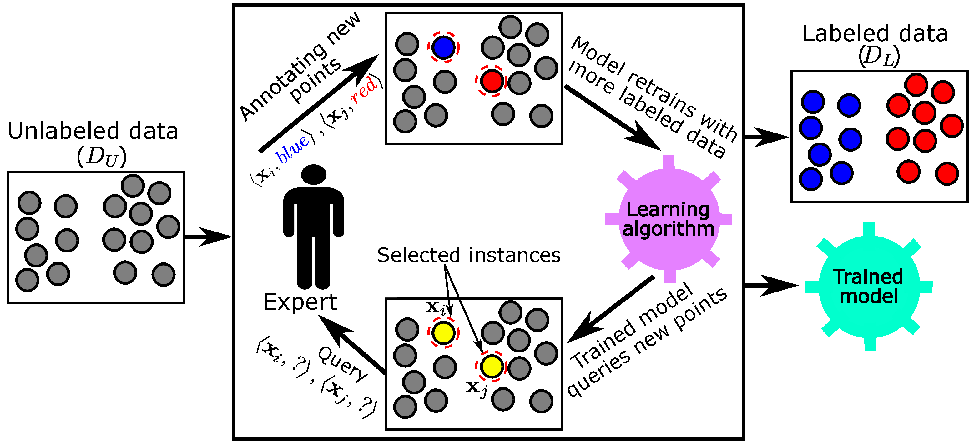
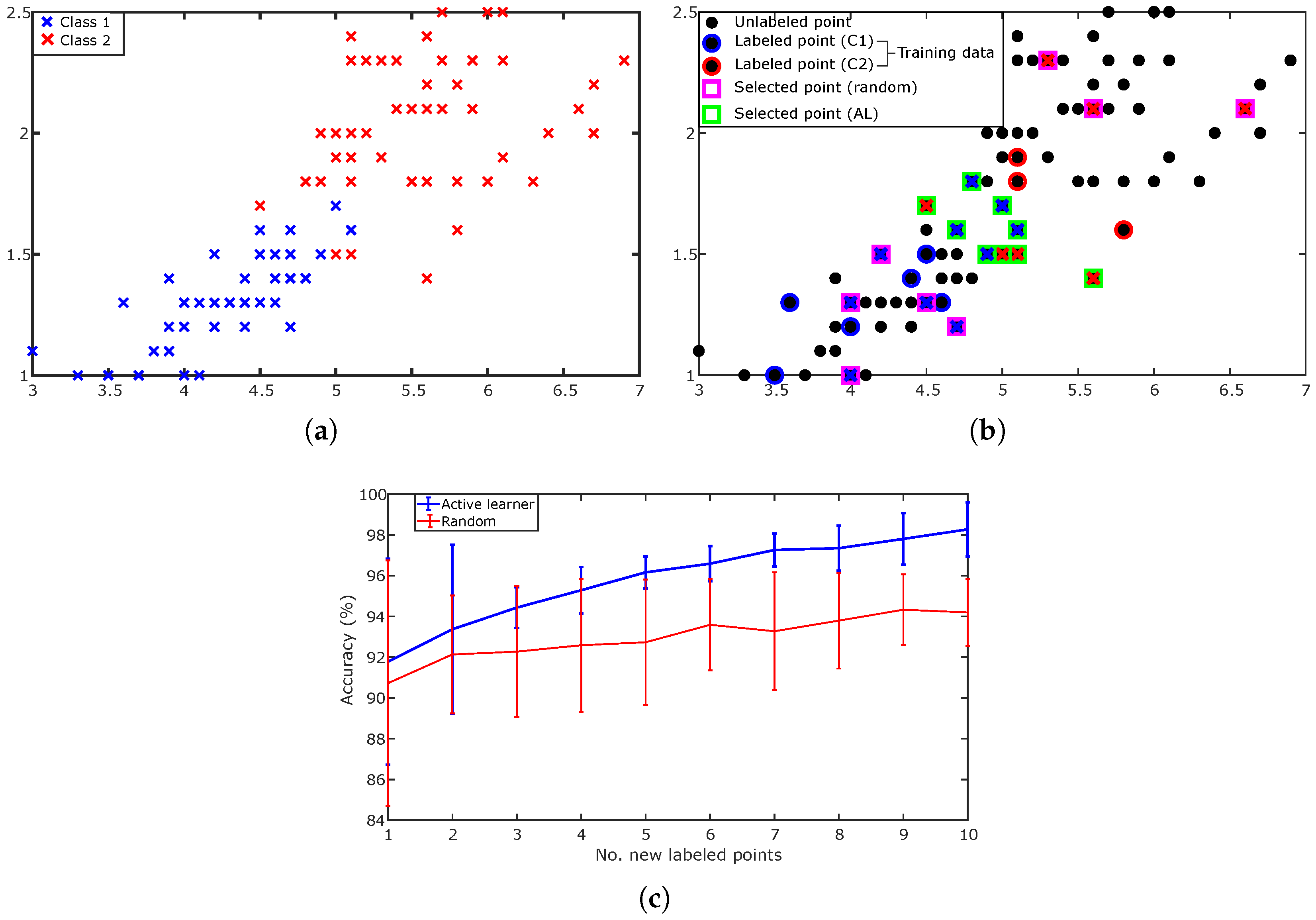
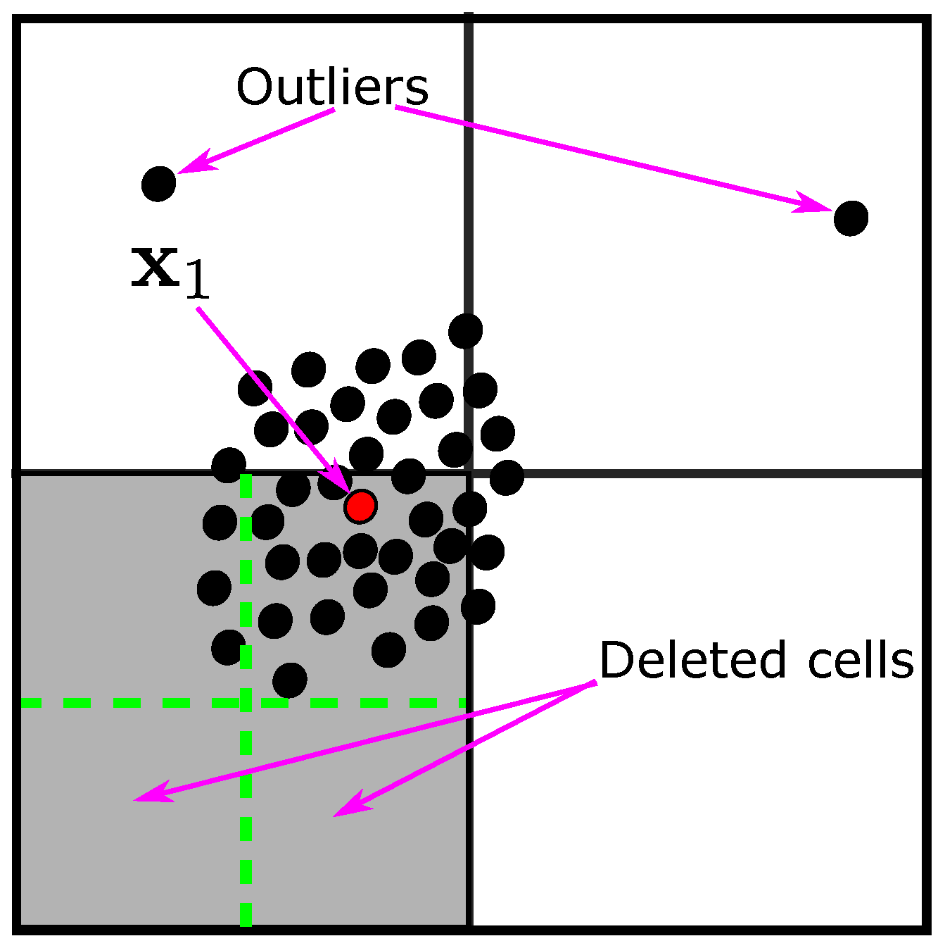
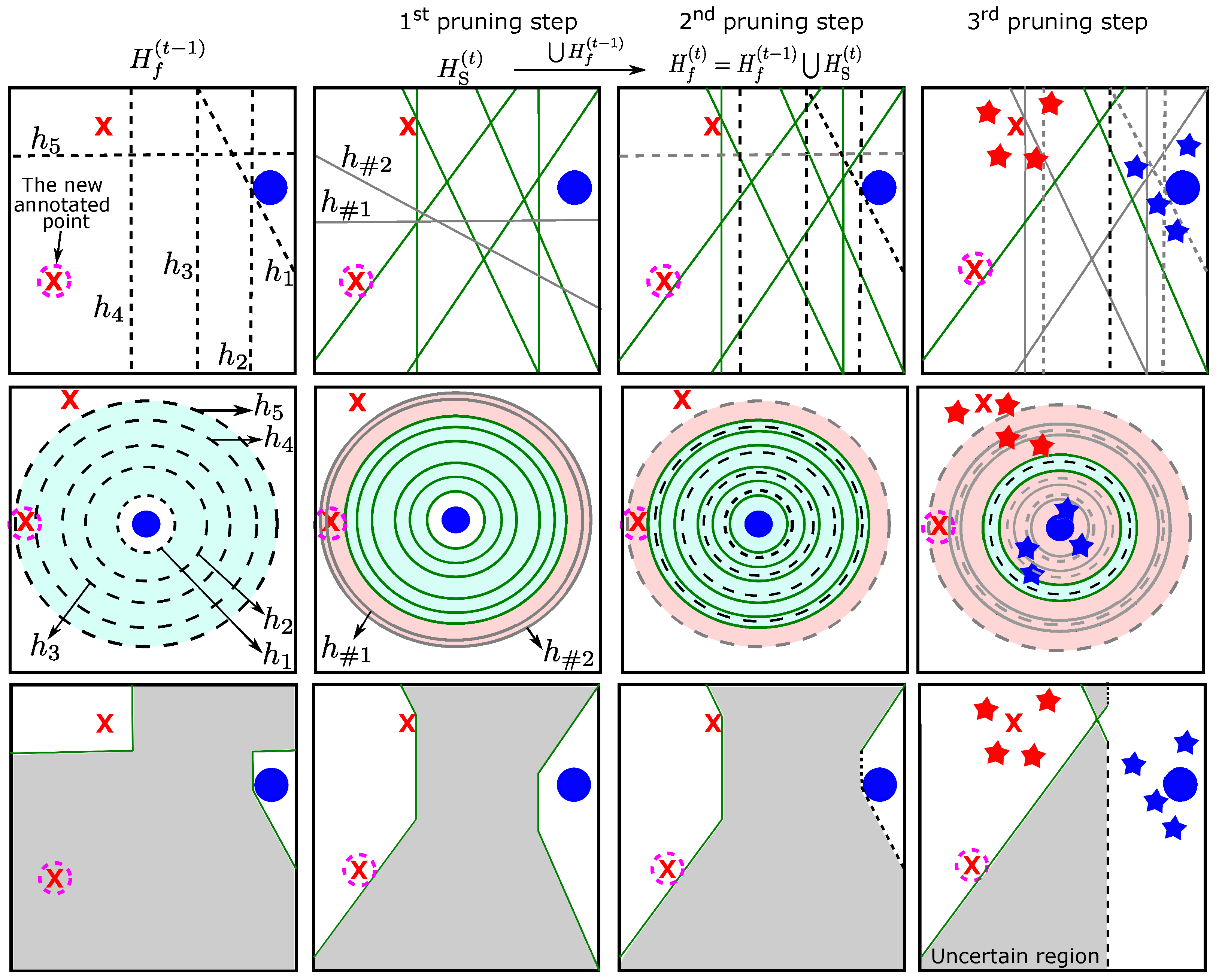
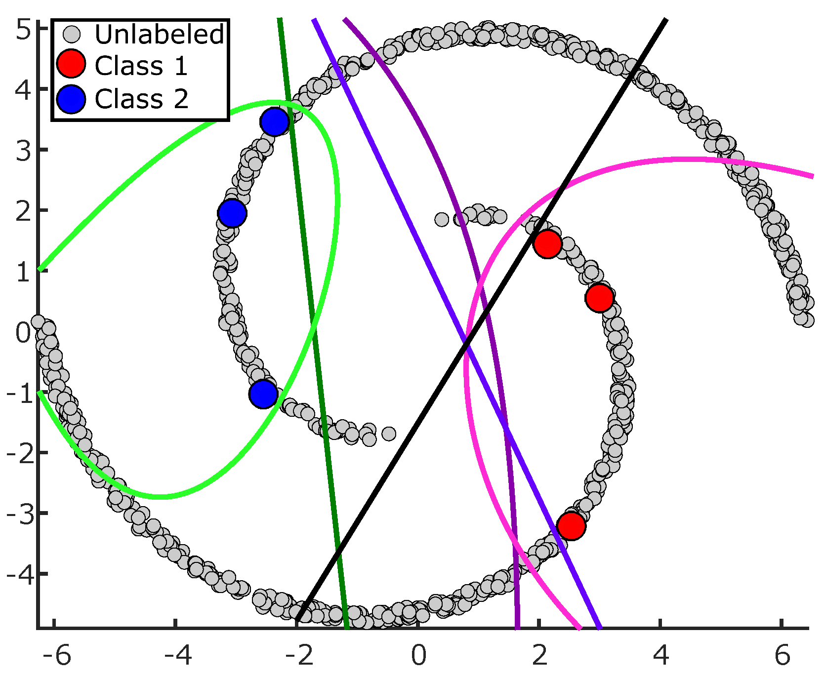
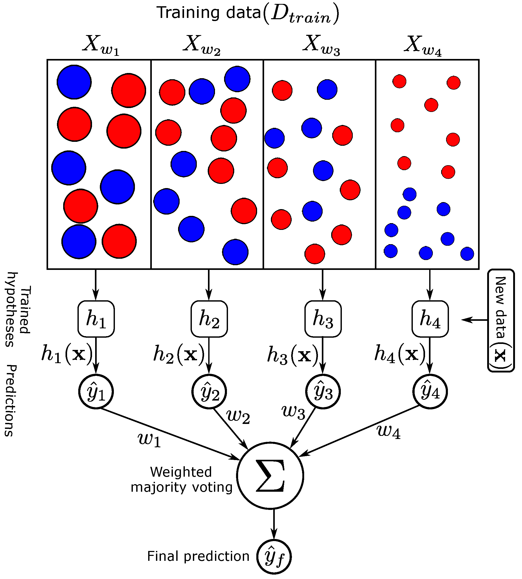
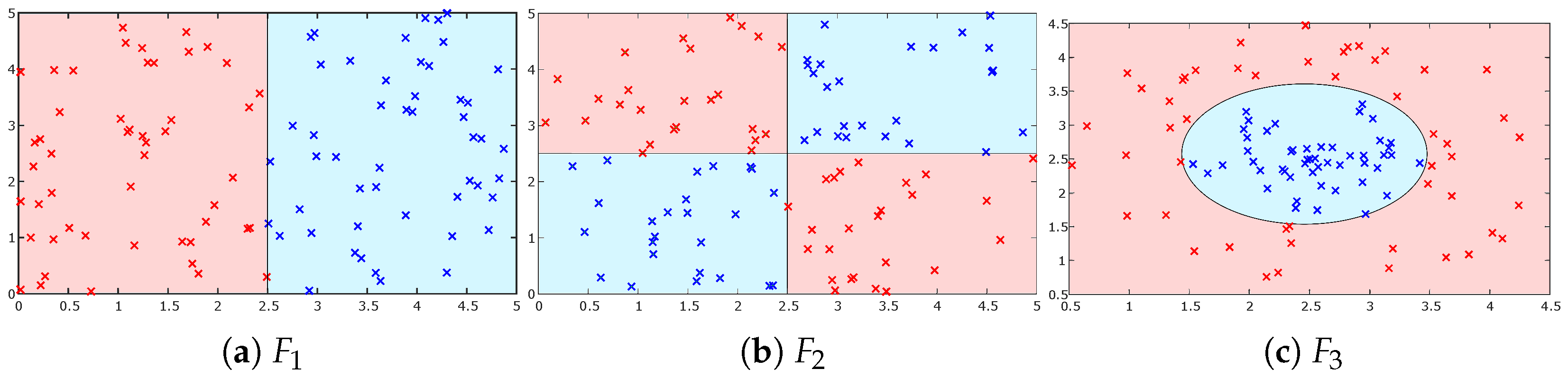
Table 1.
Notation and descriptions used in this paper.
| Notation | Meaning | Notation | Meaning |
|---|---|---|---|
| Labeled data | Unlabeled data | ||
| No. of labeled points | No. of unlabeled points | ||
| The ith data point | Label of | ||
| Q | Query budget | d | No. of dimensions of the instance space |
| t | Current iteration | C | No. of classes |
| The ith class | Lower boundaries of the space (in all dimensions) | ||
| k | No. of cells | Upper boundaries of the space (in all dimensions) | |
| No. of pseudo-labeled points | Pseudo-labeled points | ||
| No. of subdivisions in each dimension | a | Exploration-exploitation parameter | |
| The set of selected hypotheses | The set of final hypotheses in the tth iteration | ||
| The set of cells | The label for the new selected point () | ||
| The new selected/queried point | No. of hypotheses in | ||
| W | The weights of the training points | X | Input space |
| Y | The set of outcomes | Discriminant function for the class | |
| Training data | No. of selected nearest neighbors as pseudo-labeled points | ||
| The critical region in the tth iteration | The set of newly generated hypotheses in the tth iteration | ||
| A point in the critical region | The number of votes that a label receives (see Equation (4)) | ||
| The uncertainty score for the ith cell | The uncertainty score of | ||
| No. of final hypotheses in | The output of the classifier with the class | ||
| m | No. of new hypotheses trained in the exploitation phase | r | Random number |
Table 2.
Comparison between the proposed models (LQBALI and LQBALII) and the random, LLR, AOD, CB, and LHCE models using synthetic data in terms of accuracy, sensitivity, and specificity (in the form of ). The highlighted results are the best ones.
Table 2.
Comparison between the proposed models (LQBALI and LQBALII) and the random, LLR, AOD, CB, and LHCE models using synthetic data in terms of accuracy, sensitivity, and specificity (in the form of ). The highlighted results are the best ones.
| Fn. | IR | Random | LLR | AOD | CB | LHCE | LQBALI | LQBALII |
|---|---|---|---|---|---|---|---|---|
| 1:1 | 81.2(7)/76.7(5)/86.0(6) | 83.9(5)/73.1(7)/95.3(2) | 85.9(3)/74.1(6)/97.9(1) | 83.7(6)/84.6(3)/83.3(7) | 85.0(4)/82.9(4)/87.3(5) | 92.3(1)/93.1(1)/91.4(3) | 90.6(2)/92.0(2)/89.2(4) | |
| 59.0(4)/62.2(4)/56.6(6) | 60.3(3)/47.2(6)/74.0(3) | 56.4(7)/17.7(7)/91.0(1) | 58.4(5)/58.8(5)/58.9(4) | 57.7(6)/64.7(2)/51.9(7) | 60.6(2)/64.1(3)/57.6(5) | 80.3(1)/81.1(1)/79.8(2) | ||
| 57.9(3)/48.6(4)/67.8(4) | 56.8(5)/53.9(2)/60.5(6) | 50.0(7)/12.0(7)/88.0(1) | 55.2(6)/57.5(1)/53.8(7) | 57.4(4)/51.9(3)/63.6(5) | 59.1(2)/32.9(6)/86.8(2) | 64.5(1)/45.5(5)/84.7(3) | ||
| 2.33:1 | 84.5(6)/65.8(6)/92.6(6) | 84.5(5)/54.0(7)/97.7(2) | 90.3(3)/76.7(4)/96.0(4) | 69.6(7)/79.1(3)/65.6(7) | 85.6(4)/66.5(5)/93.9(5) | 94.4(2)/83.9(2)/98.9(1) | 95.3(1)/89.9(1)/97.5(3) | |
| 65.6(4)/79.7(4)/33.8(6) | 60.3(5)/59.5(6)/63.0(3) | 35.6(7)/11.3(7)/100.0(1) | 58.3(6)/62.3(5)/49.2(4) | 67.4(3)/84.1(3)/29.2(7) | 72.4(2)/88.3(1)/34.8(5) | 82.8(1)/86.6(2)/74.1(2) | ||
| 58.1(5)/50.9(5)/58.0(3) | 58.4(4)/62.5(3)/44.5(7) | 70.0(2)/0.0(7)/100.0(1) | 57.3(6)/63.0(2)/45.2(6) | 59.3(3)/49.8(6)/53.9(4) | 56.9(7)/62.0(4)/46.3(5) | 70.5(1)/70.7(1)/70.6(2) | ||
| 4:1 | 86.1(3)/50.8(6)/95.0(2) | 84.8(4)/33.7(7)/97.5(1) | 92.0(1)/83.4(3)/94.0(4) | 59.9(7)/87.5(2)/52.9(7) | 87.7(2)/61.9(5)/94.2(3) | 72.5(5.5)/ 82.5(4)/70.0(5) | 72.5(5.5)/91.5(1)/67.8(6) | |
| 77.3(1)/92.7(1)/15.5(7) | 64.2(3)/68.8(3)/46.4(4) | 27.2(7)/12.5(7)/99.9(1) | 61.4(4)/65.4(4)/45.0(5) | 74.5(2)/86.6(2)/26.4(6) | 54.1(5)/54.6(5)/52.2(3) | 53.3(6)/49.7(6)/67.3(2) | ||
| 66.8(4)/49.9(5)/52.5(4) | 63.2(7)/66.3(4)/33.2(5) | 80.0(1)/0.0(7)/100.0(1) | 66.5(5)/75.1(2)/32.9(6) | 67.0(3)/43.6(6)/61.1(3) | 66.1(6)/76.4(1)/24.8(7) | 73.7(2)/75.1(3)/68.6(2) | ||
| Avg. Rks. | 4.11/4.44/4.89 | 4.56/5.00/3.67 | 4.22/6.11/1.67 | 5.78/3.00/5.89 | 3.44/4.00/5.00 | 3.61/3.00/4.00 | 2.28/2.44/2.89 | |
Avg. Rks. (average ranks).
Table 3.
Comparison between the proposed model (LQBAL) and the random, LLR, AOD, CB, and LHCE models using synthetic data in terms of . The highlighted results are the best ones.
Table 3.
Comparison between the proposed model (LQBAL) and the random, LLR, AOD, CB, and LHCE models using synthetic data in terms of . The highlighted results are the best ones.
| Fn. | IR | Random | LLR | AOD | CB | LHCE | LQBAL |
|---|---|---|---|---|---|---|---|
| 1 | 4 | 0 | 0 | 3 | 1 | 0 | |
| 1 | 0 | 0 | 0 | 6 | 0 | ||
| 1 | 0 | 51 | 3 | 2 | 0 | ||
| 2.3 | 5 | 12 | 0 | 14 | 8 | 0 | |
| 7 | 2 | 0 | 11 | 7 | 0 | ||
| 7 | 2 | 51 | 5 | 11 | 0 | ||
| 4 | 15 | 27 | 0 | 23 | 10 | 13 | |
| 21 | 4 | 0 | 12 | 18 | 18 | ||
| 14 | 3 | 51 | 17 | 17 | 0 | ||
| Avg. NoFs | 8.33 | 5.56 | 17.00 | 9.78 | 8.89 | 4.22 | |
Table 4.
Description of the real datasets.
| Dataset | d | IR (min./maj.) | |
|---|---|---|---|
| Liver (LD1) | 345 | 6 | 1.38 (145/200) |
| Glass0 (LD2) | 214 | 5 | 2.06 (70/144) |
| Ecoli1 (LD3) | 336 | 7 | 3.36 (77/259) |
| Ecoli2 (LD4) | 336 | 7 | 5.46 (52/284) |
| Glass6 (LD5) | 214 | 5 | 6.38 (70/144) |
| Ecoli3 (LD6) | 336 | 7 | 8.6 (35/301) |
| Ecoli034vs5 (HD1) | 200 | 7 | 9 (20/180) |
| Glass016vs2 (HD2) | 192 | 9 | 10.29 (17/175) |
| Ecoli0146vs5 (HD3) | 280 | 6 | 13 (20/260) |
| Ecoli4 (HD4) | 336 | 7 | 15.8 (20/316) |
| Glass5 (HD5) | 336 | 9 | 22.78 (9/205) |
| Ecoli0137vs26 (HD6) | 281 | 7 | 39.14 (7/274) |
| Wine (MD1) | 178 | 13 | 1.5 (59/71/48) |
| New-thyroid (MD2) | 215 | 5 | 5 (30/35/150) |
| Balance (MD3) | 625 | 4 | 5.88 (49/288/288) |
| Glass (MD4) | 214 | 9 | 8.44 (70/76/17/13/9/29) |
| Ecoli (MD5) | 336 | 7 | 71.5 (143/77/20/52/5/35/2/2) |
(min./maj.)—number of minority class instances/number of majority class instances; LD. lower dataset; HD. higher dataset; MD. multiclass dataset.
Table 5.
Comparison between the proposed models (LQBALI and LQBALII) and the random, LLR, CB, and LHCE models in terms of accuracy, sensitivity, and specificity results in the form of on imbalanced datasets with IR . The highlighted results are the best ones.
Table 5.
Comparison between the proposed models (LQBALI and LQBALII) and the random, LLR, CB, and LHCE models in terms of accuracy, sensitivity, and specificity results in the form of on imbalanced datasets with IR . The highlighted results are the best ones.
| Ds. | Random | LLR | CB | LHCE | LQBALI | LQBALII |
|---|---|---|---|---|---|---|
| LD1 | 58.5(3)/48.9(2)/65.7(5) | 55.8(5)/46.8(5)/62.4(6) | 58.4(4)/48.1(4)/66.2(4) | 53.0(6)/29.2(6)/71.2(1) | 59.0(2)/48.6(3)/66.7(2) | 59.2(1)/49.4(1)/66.4(3) |
| LD2 | 63.7(5)/53.1(2)/69.3(4) | 68.0(1)/66.6(1)/68.6(5) | 64.5(4)/45.3(5)/74.3(2) | 67.0(2)/0.0(6)/100.0(1) | 59.9(6)/48.1(4)/65.5(6) | 64.8(3)/52.8(3)/70.4(3) |
| LD3 | 85.6(4)/55.5(3)/95.1(3) | 88.7(2)/55.1(4)/99.1(1) | 83.7(5)/38.9(5)/98.0(2) | 73.0(6)/5.9(6)/94.1(5) | 88.9(1)/70.0(2)/94.8(4) | 88.7(3)/73.5(1)/93.4(6) |
| LD4 | 83.1(6)/59.4(3)/90.4(5) | 83.3(3)/62.2(1)/89.3(6) | 83.2(4)/46.1(5)/94.6(2) | 83.2(5)/44.7(6)/94.8(1) | 83.9(1)/59.7(2)/91.2(4) | 83.8(2)/54.6(4)/92.5(3) |
| LD5 | 88.8(4)/56.9(4)/94.7(5) | 91.2(1.5)/61.9(3)/96.7(3) | 87.8(5)/39.9(5)/96.7(2) | 85.2(6)/7.8(6)/99.4(1) | 90.0(3)/63.1(2)/95.0(4) | 91.1(1.5)/73.9(1)/94.3(6) |
| LD6 | 89.1(6)/26.2(4)/96.5(5) | 92.0(1)/83.5(1)/93.0(6) | 89.6(5)/23.5(5)/97.4(2) | 89.7(4)/1.9(6)/99.8(1) | 91.2(3)/41.7(3)/96.8(4) | 91.9(2)/48.3(2)/96.9(3) |
| Avg. Rks. | 4.67/3.00/4.50 | 2.25/2.50/4.50 | 4.50/4.83/2.33 | 4.83/6.00/1.67 | 2.67/2.67/4.00 | 2.08/2.00/4.00 |
Table 6.
Comparison between the proposed model (LQBAL) and the random, LLR, CB, and LHCE models in terms of and (in the form of NoF/) on imbalanced datasets with IR . The highlighted results are the best ones.
Table 6.
Comparison between the proposed model (LQBAL) and the random, LLR, CB, and LHCE models in terms of and (in the form of NoF/) on imbalanced datasets with IR . The highlighted results are the best ones.
| Random | LLR | CB | LHCE | LQBAL | |
|---|---|---|---|---|---|
| LD1 | 0/7.8(1) | 0/7.0(5) | 0/7.5(2) | 0/7.3(3) | 0/7.1(4) |
| LD2 | 0/3.8(3) | 0/5.0(1) | 1/3.7(4) | 0/3.0(5) | 0/4.7(2) |
| LD3 | 1/2.8(4) | 0/3.0(1) | 6/1.6(5) | 2/2.8(3) | 0/2.9(2) |
| LD4 | 0/3.4(4) | 0/6.0(1) | 1/2.5(5) | 0/4.3(2) | 0/3.5(3) |
| LD5 | 1/2.8(1) | 0/2.0(4) | 10/1.9(5) | 2/2.5(3) | 0/2.7(2) |
| LD6 | 9/1.5(4) | 0/2.0(2) | 20/1.1(5) | 8/1.8(3) | 0/2.5(1) |
| Avg. Rks. | 1.83/2.83 | 0.00/2.33 | 6.33/4.33 | 2.00/3.17 | 0.00/2.33 |
Table 7.
Comparison between the proposed models (LQBALI and LQBALII) and the random, LLR, CB, and LHCE models in terms of accuracy, sensitivity, and specificity results in the form of on imbalanced datasets with IR . The highlighted results are the best ones.
Table 7.
Comparison between the proposed models (LQBALI and LQBALII) and the random, LLR, CB, and LHCE models in terms of accuracy, sensitivity, and specificity results in the form of on imbalanced datasets with IR . The highlighted results are the best ones.
| Ds. | Random | LLR | CB | LHCE | LQBALI | LQBALII |
|---|---|---|---|---|---|---|
| HD1 | 92.3(2)/37.0(4)/98.4(3) | 95.3(1)/57.0(1)/99.6(1) | 91.1(4)/26.3(6)/98.2(4) | 91.9(3)/30.9(5)/98.6(2) | 89.9(5)/37.2(3)/95.8(5) | 89.5(6)/41.4(2)/94.8(6) |
| HD2 | 89.3(3)/4.1(4)/97.5(3) | 86.8(4)/5.0(3)/94.7(4) | 89.6(2)/2.8(5)/98.0(2) | 90.0(1)/2.1(6)/98.3(1) | 86.4(6)/9.5(2)/93.6(5) | 86.5(5)/11.0(1)/93.6(6) |
| HD3 | 94.3(4)/33.1(5)/99.0(5) | 96.9(2)/58.7(2)/99.8(1) | 93.4(6)/16.8(6)/99.3(4) | 94.3(5)/33.5(4)/98.9(6) | 96.0(3)/48.4(3)/99.6(3) | 96.9(1)/60.4(1)/99.6(2) |
| HD4 | 95.2(4)/28.3(4)/99.4(3) | 94.0(6)/0.0(6)/100.0(1) | 94.8(5)/15.6(5)/99.8(2) | 95.6(3)/37.8(3)/99.3(4) | 97.7(1)/75.8(2)/98.9(5) | 97.2(2)/79.8(1)/98.3(6) |
| HD5 | 95.2(5)/10.6(4)/98.9(3) | 95.8(3)/0.0(6)/100.0(1) | 95.0(6)/7.4(5)/98.8(4) | 95.5(4)/10.6(3)/99.1(2) | 96.8(1)/50.0(2)/98.4(5) | 96.6(2)/67.7(1)/97.7(6) |
| HD6 | 97.5(4)/19.7(3)/99.4(6) | 97.5(6)/0.0(6)/100.0(1) | 97.6(3)/4.7(5)/99.9(2) | 97.5(5)/11.9(4)/99.6(4) | 98.0(1)/22.9(2)/99.7(3) | 97.9(2)/29.1(1)/99.5(5) |
| Avg. Rks. | 3.67/4.00/3.83 | 3.67/4.00/1.50 | 4.33/5.33/3.00 | 3.50/4.17/3.17 | 2.83/2.33/4.33 | 3.00/1.17/5.17 |
Table 8.
Comparison between the proposed model (LQBAL) and the random, LLR, CB, and LHCE models in terms of NoF and (in the form of NoF/) on imbalanced datasets with IR . The highlighted results are the best ones.
Table 8.
Comparison between the proposed model (LQBAL) and the random, LLR, CB, and LHCE models in terms of NoF and (in the form of NoF/) on imbalanced datasets with IR . The highlighted results are the best ones.
| Random | LLR | CB | LHCE | LQBAL | |
|---|---|---|---|---|---|
| HD1 | 15/1.1(1) | 0/1.0(3.5) | 21/0.9(5) | 17/1.1(2) | 0/1.0(3.5) |
| HD2 | 23/0.8(4.5) | 0/1.0(3) | 23/0.8(4.5) | 17/1.0(2) | 0/1.5(1) |
| HD3 | 20/1.0(3) | 0/1.0(4) | 29/0.6(5) | 14/1.3(2) | 0/1.7(1) |
| HD4 | 17/0.9(3) | 51/0.0(5) | 34/0.4(4) | 21/1.1(2) | 0/2.2(1) |
| HD5 | 16/0.9(3) | 51/0.0(5) | 32/0.5(4) | 18/1.0(2) | 0/3.0(1) |
| HD6 | 13/1.3(2) | 0/1.0(3) | 37/0.4(5) | 22/1.0(4) | 0/1.9(1) |
| Avg. Rks. | 17.33/2.75 | 17.00/3.92 | 29.33/4.58 | 18.17/2.33 | 0.00/1.42 |
Table 9.
Comparison between the proposed model (LQBAL) and the random, LLR, CB, and LHCE models with multi-class imbalanced datasets, query budget 5%, and in terms of the number of annotated points from each class. The highlighted results represent the results of the minority class(es), and each minority class has a different color (if there is more than one minority class).
| Ds. | Random | LLR | CB | LHCE | LQBAL |
|---|---|---|---|---|---|
| MD1 | 2.9/3.7/2.5 | 9.0/0.0/0.0 | 2.8/3.5/2.7 | 2.9/3.8/2.2 | 3.1/3.1/2.8 |
| MD2 | 1.4/1.8/7.8 | 3.0/2.0/6.0 | 1.8/2.0/7.2 | 1.9/2.4/6.7 | 2.2/2.0/6.7 |
| MD3 | 2.4/14.3/15.3 | 2.5/15.2/14.3 | 2.7/14.6/14.7 | 3.4/13.7/14.9 | 8.1/12.2/11.8 |
| MD4 | 3.8/3.9/0.7/0.7/0.5/1.4 | 5.0/4.0/0.0/0.0/0.0/2.0 | 3.5/3.7/1.1/0.5/0.7/1.5 | 4.4/4.2/0.6/0.5/0.3/1.1 | 4.7/3.9/0.1/0.2/1.0/1.1 |
| MD5* | 1.0/0.3/0.1/0.1 | 0.0/1.0/0.0/0.0 | 1.2/0.2/0.1/0.1 | 0.9/0.2/0.0/0.1 | 1.8/0.0/0.0/0.0 |
| TMPs | 11.5 | 8.5 | 13.1 | 12.5 | 18.2 |
TMPs: total number of minority points. MD5*: with MD5, we present only the results of the minority classes and neglect the results of the majority classes because all algorithms succeeded at finding points from majority classes.
Table 10.
Comparison between the proposed model (LQBAL) and the random, LLR, CB, and LHCE models with multi-class imbalanced datasets, query budget 10%, and in terms of the number of annotated points from each class. The highlighted results represent the results of the minority class(es), and each minority class has a different color (if there is more than one minority class).
| Ds. | Random | LLR | CB | LHCE | LQBAL |
|---|---|---|---|---|---|
| MD1 | 5.7/7.4/4.9 | 15.0/0.0/3.0 | 5.5/7.5/5.0 | 2.9/3.8/2.2 | 5.4/7.1/5.5 |
| MD2 | 3.5/3.5/15.0 | 3.0/5.0/14.0 | 3.2/2.9/15.9 | 1.9/2.4/6.7 | 3.2/4.7/14.2 |
| MD3 | 5.3/29.5/28.1 | 5.6/29.9/27.6 | 5.3/28.6/29.1 | 3.4/13.7/14.9 | 13.3/21.3/28.4 |
| MD4 | 7.5/8.2/1.8/1.0/0.9/2.6 | 8.0/8.0/1.0/2.0/0.0/3.0 | 7.2/8.3/1.4/1.3/1.1/2.8 | 4.4/4.2/0.6/0.5/0.3/1.1 | 5.4/9.4/0.8/1.2/1.9/3.4 |
| MD5* | 2.0/0.5/0.3/0.2 | 2.0/2.0/0.0/0.0 | 2.5/0.6/0.2/0.3 | 0.9/0.2/0.0/0.1 | 2.5/0.1/0.0/0.0 |
| TMPs | 23.7 | 23.6 | 23.8 | 12.5 | 33.2 |
TMPs: total number of minority points. MD5*: for MD5, we present only the results of the minority classes and neglect the results of the majority classes because all algorithms succeeded in finding points from majority classes.
Table 11.
The numbers of labeled data ( and ), correct PLs ( and ), false/noisy PLs ( and ), and conflict points () of the proposed model (LQBALII) on higher imbalanced datasets.
Table 11.
The numbers of labeled data ( and ), correct PLs ( and ), false/noisy PLs ( and ), and conflict points () of the proposed model (LQBALII) on higher imbalanced datasets.
| Ds. | Pseudo-Labeled Points () | ||||||
|---|---|---|---|---|---|---|---|
| HD1 | 1 | 9 | 1 | 17 | 1 | 0 | 0 |
| HD2 | 1.5 | 9.5 | 1.3 | 17.7 | 1.3 | 0.3 | 9 |
| HD3 | 1.7 | 12.3 | 2.3 | 34.3 | 0 | 1.3 | 18 |
| HD4 | 2.2 | 14.8 | 5.7 | 57.3 | 2 | 0.7 | 0 |
| HD5 | 3.0 | 20 | 3.3 | 52.3 | 1.7 | 0 | 63 |
| HD6 | 1.9 | 38.1 | 1.3 | 89.3 | 0.7 | 1.3 | 169.3 |
Publisher’s Note: MDPI stays neutral with regard to jurisdictional claims in published maps and institutional affiliations. |
© 2022 by the authors. Licensee MDPI, Basel, Switzerland. This article is an open access article distributed under the terms and conditions of the Creative Commons Attribution (CC BY) license (https://creativecommons.org/licenses/by/4.0/).
Share and Cite
MDPI and ACS Style
Tharwat, A.; Schenck, W. A Novel Low-Query-Budget Active Learner with Pseudo-Labels for Imbalanced Data. Mathematics 2022, 10, 1068. https://doi.org/10.3390/math10071068
AMA Style
Tharwat A, Schenck W. A Novel Low-Query-Budget Active Learner with Pseudo-Labels for Imbalanced Data. Mathematics. 2022; 10(7):1068. https://doi.org/10.3390/math10071068
Chicago/Turabian StyleTharwat, Alaa, and Wolfram Schenck. 2022. "A Novel Low-Query-Budget Active Learner with Pseudo-Labels for Imbalanced Data" Mathematics 10, no. 7: 1068. https://doi.org/10.3390/math10071068
Note that from the first issue of 2016, this journal uses article numbers instead of page numbers. See further details here.