Domination Coloring of Graphs

Abstract

A domination coloring of a graph G is a proper vertex coloring of G, such that each vertex of G dominates at least one color class (possibly its own class), and each color class is dominated by at least one vertex. The minimum number of colors among all domination colorings is called the domination chromatic number, denoted by ${\chi }_{dd}\left(G\right)$. In this paper, we study the complexity of the k-domination coloring problem by proving its NP-completeness for arbitrary graphs. We give basic results and properties of ${\chi }_{dd}\left(G\right)$, including the bounds and characterization results, and further research ${\chi }_{dd}\left(G\right)$ of some special classes of graphs, such as the split graphs, the generalized Petersen graphs, corona products, and edge corona products. Several results on graphs with ${\chi }_{dd}\left(G\right)=\chi \left(G\right)$ are presented. Moreover, an application of domination colorings in social networks is proposed.

1. Introduction and Preliminary

1.1. Introduction

Coloring and domination are two important fields in graph theory, and both have rich research results. For comprehensive results of coloring and domination in graphs, refer to [1,2,3,4,5,6,7,8,9,10,11,12,13,14,15,16,17], respectively. Moreover, graph coloring and domination problems are often in relation. Chellali and Volkmann [18] showed some relations between the chromatic number and some domination parameters in a graph. For a graph $G=(V,E)$, a vertex $v\in V$ dominates a set $S\subseteq V$ if it is adjacent to every vertex of S, meanwhile, we say that v is a dominator of S, and S is dominated by v. Hedetniemi et al. [19] introduced the concept of a dominator partition of a graph. A dominator partition is a partition $\pi =\{V_1,V_2,\cdots ,V_k\}$ of $V\left(G\right)$, such that every vertex $v\in V$ is a dominator of at least one block $V_i$ of $\pi$. Motivated by [19], Gera et al. [20] proposed the dominator coloring in 2006.

Definition 1

([20]). A dominator coloring of a graph G is a proper coloring, such that every vertex of G dominates at least one color class (possibly its own class). The dominator chromatic number of G, denoted by ${\chi }_d\left(G\right)$, is the minimum number of colors among all dominator colorings of G.

Gera researched further in [21,22]. More results on the dominator coloring can be found in [23,24,25,26]. Kazemi [27] proposed the concept of total dominator coloring in 2015, which is a proper coloring, such that each vertex of the graph is adjacent to every vertex of some (other) color class. For more results on the total dominator coloring, refer to [28,29,30]. In 2015, Merouane et al. [31] proposed the dominated coloring:

Definition 2

([31]). A dominated coloring of a graph G is a proper coloring such that every color class is dominated by at least one vertex. The dominated chromatic number of G, denoted by ${\chi }_{dom}\left(G\right)$, is the minimum number of colors among all dominated colorings of G.

More results on the dominated coloring can be found in [32,33,34].

For problems mentioned above, the domination property is defined either on vertices or on color classes. Indeed, each color class in a dominator coloring is not necessarily dominated by a vertex, and each vertex in a dominated coloring does not necessarily dominate a color class. In this paper, we introduce the domination coloring that both of the vertices and color classes should satisfy the domination property.

Definition 3.

A domination coloring of a graph G is a proper vertex coloring of G, such that each vertex of G dominates at least one color class (possibly its own class), and each color class is dominated by at least one vertex. The domination chromatic number of G, denoted by ${\chi }_{dd}\left(G\right)$, is the minimum number of color classes in a domination coloring of G.

The domination coloring problem is to find a domination coloring of G, such that the number of color classes is minimized. Here, we describe a possible application for the domination coloring problem in the following scenario. In a social network, social actors are represented as vertices and their relationships as edges (two actors are adjacent if they are friends). Two strangers can become friends by their mutual friend (i.e., intermediary). Then, each actor wants to develop interpersonal relationships in the social network by some intermediaries, meanwhile, each actor wants to be the important intermediary of other strangers. The domination coloring problem involves finding the minimum groups of actors in the social network with the below properties:

• Actors in the same group are strangers;
• Actors in the same group can become friends by at least one common intermediary;
• Each actor is an intermediary of at least one actor (stranger) group.

We proceed as follows. In the rest of Section 1, we recall some basic definitions that will be used in the following sections. In Section 2, we analyse the complexity of the k-domination coloring problem. In Section 3, we present basic results and properties of the domination chromatic number ${\chi }_{dd}\left(G\right)$, including the bounds and characterization results. In Section 4, we further research ${\chi }_{dd}\left(G\right)$ of some special classes of graphs, including the split graphs, the generalized Petersen graphs $P(n,1)$, corona products, and edge corona products. In Section 5, we investigate some realization results on graphs with ${\chi }_{dd}\left(G\right)=\chi \left(G\right)$. Finally, we make a conclusion in Section 6.

1.2. Preliminary

Graphs considered in this paper are finite, simple, undirected, and connected. Let $G=(V,E)$ be a graph with $n=\left|V\right|$ and $m=\left|E\right|$. For any vertex $v\in V\left(G\right)$, the open neighborhood of v is the set $N\left(v\right)=\left\{u\right|uv\in E\left(G\right)\}$ and the closed neighborhood is the set $N\left[v\right]=N\left(v\right)\cup \left\{v\right\}$. Similarly, the open and closed neighborhoods of a set $X\subseteq V$ are, respectively, $N\left(X\right)={\bigcup }_{x\in X}N\left(x\right)$ and $N\left[X\right]=N\left(X\right)\cup X$. The degree of a vertex $v\in V$, denoted by $deg\left(v\right)$, is the cardinality of its open neighborhood. The maximum and minimum degree of a graph G is denoted by $\Delta \left(G\right)$ and $\delta \left(G\right)$, respectively. We call a vertex of degree one a leaf or a pendant vertex, its adjacent vertex a support vertex. Given a set $X\subseteq V$, we denote by $G\left[X\right]$ the subgraph of G induced by X. Given any graph H, a graph G is H-free if it does not have any induced subgraph isomorphic to H. We denote by $P_n$ the path on n vertices and by $C_n$ the cycle on n vertices. A tree is a connected acyclic graph. The complete graph on n vertices is denoted by $K_n$ and the complete graph of order 3 is called a triangle. The complete bipartite graph with classes of orders r and s is denoted by $K_{r,s}$. A star $S_k$ is the graph $K_{1,k}$ with $k\ge 1$.

An independent set in G is a set of vertices, such that any two vertices in the set are not adjacent. A matching in a graph G is a set of nonadjacent edges of G. The matching number ${\alpha }^{\prime }\left(G\right)$ is the cardinality of a largest matching in G. A vertex cover in a graph G is a set of vertices, such that each edge has at least one endpoint in the set. The vertex cover number $\beta \left(G\right)$ is the cardinality of a smallest vertex cover in G. The clique number $w\left(G\right)$ of a graph G is the maximum order among the complete subgraphs of G.

A proper vertex k-coloring of a graph $G=(V,E)$ is a mapping $f:V\to \{1,2,\cdots ,k\}$, such that any two adjacent vertices receive different colors. In fact, this problem is equivalent to the problem of partitioning the vertex set of G into k independent sets $\{V_1,V_2,\cdots ,V_k\}$ where $V_i=\{x\in V|f\left(x\right)=i\}$. The set of all vertices colored with the same color is called a color class. The chromatic number of G, denoted by $\chi \left(G\right)$, is the minimum number of colors among all proper colorings of G.

A dominating set S is a subset of the vertices in a graph G, such that every vertex in G either belongs to S or has a neighbor in S. The domination number $\gamma \left(G\right)$ is the minimum cardinality of a dominating set of G. A $\gamma \left(G\right)$-set is a dominating set of G with minimum cardinality.

For any undefined terms, the reader is referred to the book by Bondy and Murty [35].

2. Complexity Results

This section focuses on the complexity study of the domination coloring problem, e.g., whether an arbitrary graph admits a domination coloring with the most k colors. We give the formalization of this problem.

• k-domination coloring problem.
  Instance: a graph $G=(V,E)$ without isolated vertices and a positive integer k.
  Question: is there a domination coloring of G with the most k colors?

Theorem 1.

For $k\ge 4$, the k-domination coloring problem is NP-complete.

 Proof. 

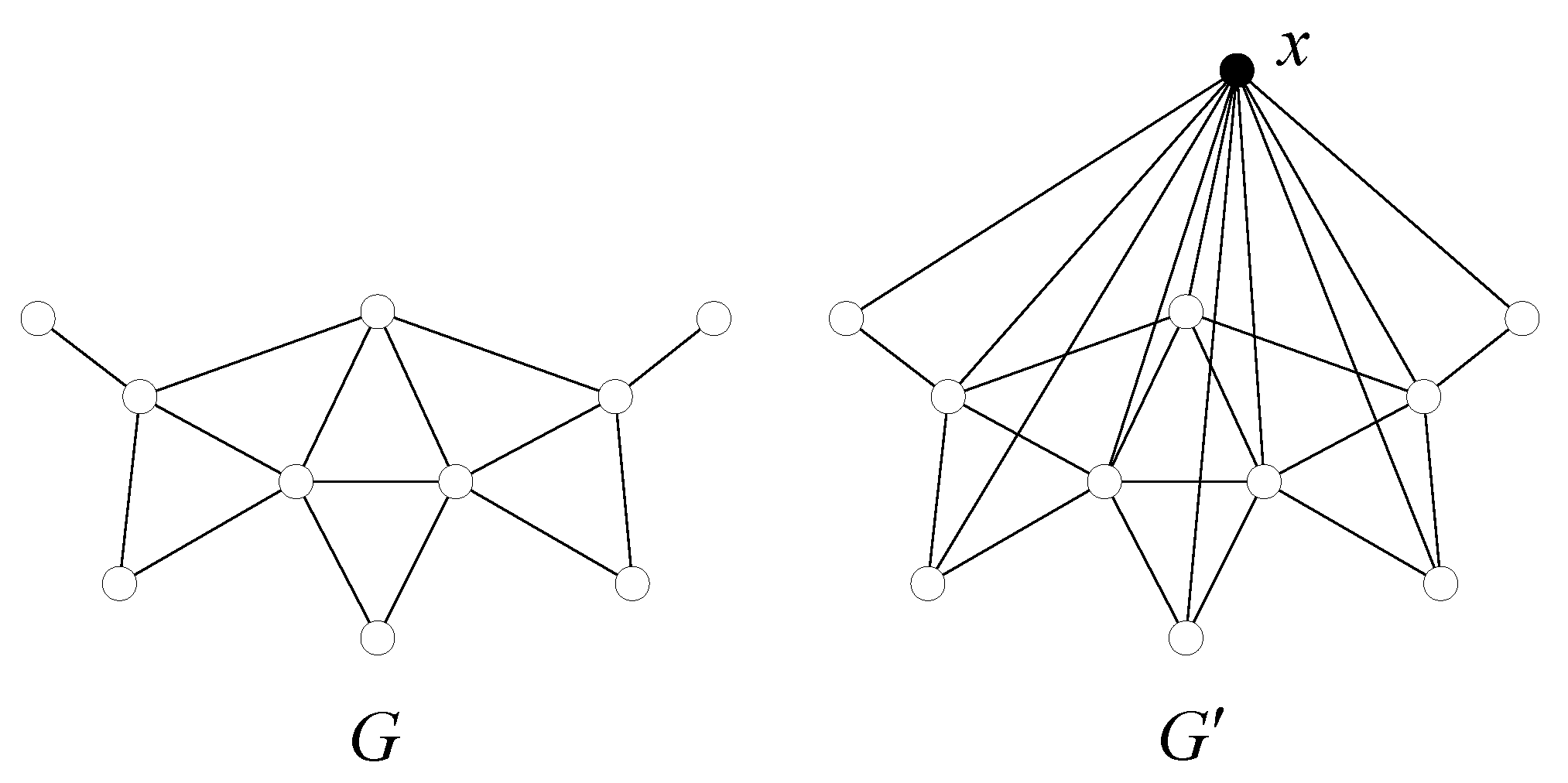
The k-domination coloring problem is in NP, since verifying if a coloring is a domination coloring could be performed in polynomial time. Now, we give a polynomial time reduction from the k-coloring problem, which is known to be NP-complete, for $k\ge 3$. Let $G=(V,E)$ be a graph without isolated vertices. We construct a graph $G^{\prime }$ from G by adding a new vertex x to G and adding edges between x and every vertex of G. That is, x is a dominating vertex of $G^{\prime }$, as shown in Figure 1. We show that G admits a proper coloring with k colors if and only if $G^{\prime }$ admits a domination coloring with $k+1$ colors.

First, we prove the necessity. Let f be a proper k-coloring of G, and the corresponding color classes set is $\{V_1,V_2,\cdots ,V_k\}$. We construct a $(k+1)$-domination coloring $f^{\prime }$ of $G^{\prime }$ with the color classes set $\{V_1^{{}^{\prime }}=V_1,V_2^{{}^{\prime }}=V_2,\cdots ,V_k^{{}^{\prime }}=V_k,V_{k+1}^{{}^{\prime }}=\left\{x\right\}\}$. It is easy to see that $f^{\prime }$ is a domination coloring of $G^{\prime }$ since

• $f^{\prime }$ is proper;
• Each vertex other than x dominates at least the color class containing x and x dominates all color classes of $f^{\prime }$;
• Each color class other than $\left\{x\right\}$ is dominated by x and the color class containing x is dominated by any other vertex.

Then, we prove the sufficiency. Let $f^{\prime }$ be a $(k+1)$-domination coloring of $G^{\prime }$, and $\{V_1^{{}^{\prime }},V_2^{{}^{\prime }},\cdots ,V_k^{{}^{\prime }},V_{k+1}^{{}^{\prime }}\}$ is the color classes set. Since $f^{\prime }$ is proper, there exists a color class $V_i^{{}^{\prime }}$ such that $V_i^{{}^{\prime }}=\left\{x\right\}$. Thus, we can construct a proper k-coloring of G by removing the color class $V_i^{{}^{\prime }}$ from $f^{\prime }$.

From the above, the k-domination coloring problem is NP-complete, for $k\ge 4$. □

3. Basic Results and Properties of the Domination Chromatic Number

In this section, we study some properties of the domination coloring and basic results on typical classes of graphs.

Let G be a connected graph with order $n\ge 2$. Then at least two different colors are needed in a domination coloring since there are at least two vertices in G adjacent to each other. Moreover, if each vertex receives a unique color, then both the vertices and color classes satisfy the domination property. Clearly, we get a domination coloring of G with n colors. Thus,

$$2\le {\chi }_{dd}\left(G\right)\le n.$$

(1)

Gera et al. [20] introduced the Inequalities (2) for the dominator chromatic number ${\chi }_d\left(G\right)$ and Merouane et al. [31] obtained Inequalities (3) for the dominated chromatic number ${\chi }_{dom}\left(G\right)$. Moreover, we can get a similar inequality for the domination chromatic number ${\chi }_{dd}\left(G\right)$.

$$\max \{\chi \left(G\right),\gamma \left(G\right)\}\le {\chi }_d\left(G\right)\le \chi \left(G\right)+\gamma \left(G\right).$$

(2)

$$\max \{\chi \left(G\right),\gamma \left(G\right)\}\le {\chi }_{dom}\left(G\right)\le \chi \left(G\right)·\gamma \left(G\right).$$

(3)

Proposition 1.

Let G be a graph without isolated vertices, then

$$\max \{\chi \left(G\right),\gamma \left(G\right)\}\le \max \{{\chi }_d\left(G\right),{\chi }_{dom}\left(G\right)\}\le {\chi }_{dd}\left(G\right)\le \chi \left(G\right)·\gamma \left(G\right).$$

Proof. 

Since any domination coloring of G is also a dominator coloring and a dominated coloring, $\max \{{\chi }_d\left(G\right),{\chi }_{dom}\left(G\right)\}\le {\chi }_{dd}\left(G\right)$. Both the dominator coloring and dominated coloring are proper vertex colorings of G, so, $\chi \left(G\right)\le \max \{{\chi }_d\left(G\right),{\chi }_{dom}\left(G\right)\}$. For any dominator coloring (dominated coloring) of G, we can get a dominating set by taking a vertex in each color class. Thus, $\gamma \left(G\right)\le \max \{{\chi }_d\left(G\right),{\chi }_{dom}\left(G\right)\}$. Therefore, the left two parts of the inequality hold.

For the right part of the inequality, we consider a $\gamma \left(G\right)$-set D of G. A domination coloring of G can be obtained by giving distinct colors to each vertex x of D and at most $\chi \left(G\right)-1$ new colors to the vertices of $N\left(x\right)$. Hence, we totally use at most $\gamma \left(G\right)+\left(\chi \right(G)-1)·\gamma \left(G\right)=\chi \left(G\right)·\gamma \left(G\right)$ colors. So, ${\chi }_{dd}\left(G\right)\le \chi \left(G\right)·\gamma \left(G\right)$. □

The bound of Proposition 1 is tight for complete graphs. Since every planar graph is “4-colorable” [2,3], the following result is straightforward:

Corollary 1.

Let G be a planar graph without isolated vertices, then ${\chi }_{dd}\left(G\right)\le 4\gamma \left(G\right)$.

Proposition 2.

Let G be a connected graph with order n and maximum degree Δ, then ${\chi }_{dd}\left(G\right)\ge \frac{n}{\Delta }$.

Proof. 

Consider a minimum domination coloring of G. Since G is $S_{\Delta +1}$-free, any color class would not have more than $\Delta$ vertices; otherwise, a vertex dominating such a color class will induce a star of order at least $\Delta +2$, a contradiction. So, ${\chi }_{dd}\left(G\right)\ge \frac{n}{\Delta }$. □

Theorem 2.

Let G be a connected triangle-free graph, then ${\chi }_{dd}\left(G\right)\le 2\gamma \left(G\right)$.

Proof. 

Consider a minimum dominating set S of G. Color every vertex of S with a new color. Since G does not contain any triangle, the set of neighbors of every vertex of S is an independent set. Thus, a second new color is given for each neighborhood. Obviously, this is a proper coloring of G with $2\left|S\right|$ colors, which satisfies that every vertex dominates at least one color class, and every color class is dominated by at least one vertex. Thus, ${\chi }_{dd}\left(G\right)\le 2\gamma \left(G\right)$. □

Theorem 3. 

(1) For the path $P_n$, $n\ge 2$,

$${\chi }_{dd}\left(P_n\right)=2·\lfloor \frac{n}{3}\rfloor +\mathrm{mod}(n,3);$$

(2) For the cycle $C_n$,

$${\chi }_{dd}\left(C_n\right)=\left\{\begin{array}{cc}2,\hfill & n=4,\hfill \\ 3,\hfill & n=3,5,\hfill \\ 2·\lfloor \frac{n}{3}\rfloor +\mathrm{mod}(n,3),\hfill & otherwise;\hfill \end{array}\right.$$

(3) For the complete graph $K_n$, ${\chi }_{dd}\left(K_n\right)=n$;

(4) For the complete k-partite graph $K_{a_1,a_2,\cdots ,a_k}$, ${\chi }_{dd}\left(K_{a_1,a_2,\cdots ,a_k}\right)=k$;

(5) For the complete bipartite graph $K_{r,s}$, ${\chi }_{dd}\left(K_{r,s}\right)=2$;

(6) For the star $K_{1,n}$, ${\chi }_{dd}\left(K_{1,n}\right)=2$;

(7) For the wheel $W_{1,n}$,

$${\chi }_{dd}\left(W_{1,n}\right)=\left\{\begin{array}{cc}3,\hfill & niseven,\hfill \\ 4,\hfill & nisodd.\hfill \end{array}\right.$$

Proof. 

(1) Let $P_n=v_1{v}_2\cdots v_n$. By the definition of the domination coloring, we discover that at most two non-adjacent vertices are allowed in a color class, if not, there exist no vertex dominating this color class. On the other hand, the vertex adjacent to both vertices of a color class must be the unique vertex of some color class. For convenience, let $P_5=v_1{v}_2{v}_3{v}_4{v}_5$ be a $P_5$-subgraph of $P_n$. If vertices $v_1$ and $v_3$ are in a color class, then $v_2$ must be the unique vertex of a color class. If not, $v_2$ and $v_4$ are partitioned in a color class, which will result in $v_4$ cannot dominate any color class. Thus, every three vertices of $P_n$ need to be partitioned in two color classes, and the rest form their own color class. Clearly, it is an optimal domination coloring of $P_n$. Thus, ${\chi }_{dd}\left(P_n\right)=2·\lfloor \frac{n}{3}\rfloor +\mathrm{mod}(n,3)$.

(2) For $n=3,4,5$, the result follows by inspection. For $n\ge 6$, it is not hard to find the case is similar to the path $P_n$. As the discussion in (1), the result follows.

(3) For the complete graph $K_n$, $\chi \left(K_n\right)=n$. By Proposition 1 and in Equation (1), ${\chi }_{dd}\left(K_n\right)=n$.

(4) Let $K_{a_1,a_2,\cdots ,a_k}$ be the complete k-partite graph, and $V_i(1\le i\le k)$ be the k-partite sets. Then ${\chi }_{dd}\left(K_{a_1,a_2,\cdots ,a_k}\right)\ge \chi \left(K_{a_1,a_2,\cdots ,a_k}\right)=k$. Moreover, the coloring that assigns color i to each partite set $V_i(1\le i\le k)$ is a domination coloring. The result follows.

(5) and (6) are special cases of (4).

(7) Let $W_{1,n}$ be the wheel with order $n+1$. Since,

$$\chi \left(W_{1,n}\right)=\left\{\begin{array}{cc}3,\hfill & niseven,\hfill \\ 4,\hfill & nisodd.\hfill \end{array}\right.$$

and the corresponding proper colorings are also domination colorings, the result follows. □

Note. For a given graph G, and a subgraph H of G, the domination chromatic number of H can be smaller or larger than the domination chromatic number of G. That is to say, induction may be not useful when we want to find the domination chromatic number of a graph. As an example, consider the graph $G=K_n$ and $H=P_2$, then ${\chi }_{dd}\left(K_n\right)=n\ge 2={\chi }_{dd}\left(P_2\right)$, and consider the graph $G=K_{n,n}$ and $H=P_{2n}$, then ${\chi }_{dd}\left(K_{n,n}\right)=2\le 2·\lfloor \frac{2n}{3}\rfloor +\mathrm{mod}(2n,3)={\chi }_{dd}\left(P_{2n}\right)$.

Theorem 4.

For the Petersen graph P, ${\chi }_{dd}\left(P\right)=5$.

Proof. 

It is easy to check $\{\{v_1,v_2,v_9\},\{v_3,v_4,v_6\},\{v_5,v_7\},\left\{v_8\right\},\left\{v_{10}\right\}\}$ is a domination coloring of the Petersen graph, as shown in Figure 2. So, ${\chi }_{dd}\left(P\right)\le 5$. By Proposition 2.1 in [32], ${\chi }_{dom}\left(P\right)=4$ and ${\chi }_d\left(P\right)=5$. Then, ${\chi }_{dd}\left(P\right)\ge 5$ by Proposition 1. Therefore, ${\chi }_{dd}\left(P\right)=5$. □

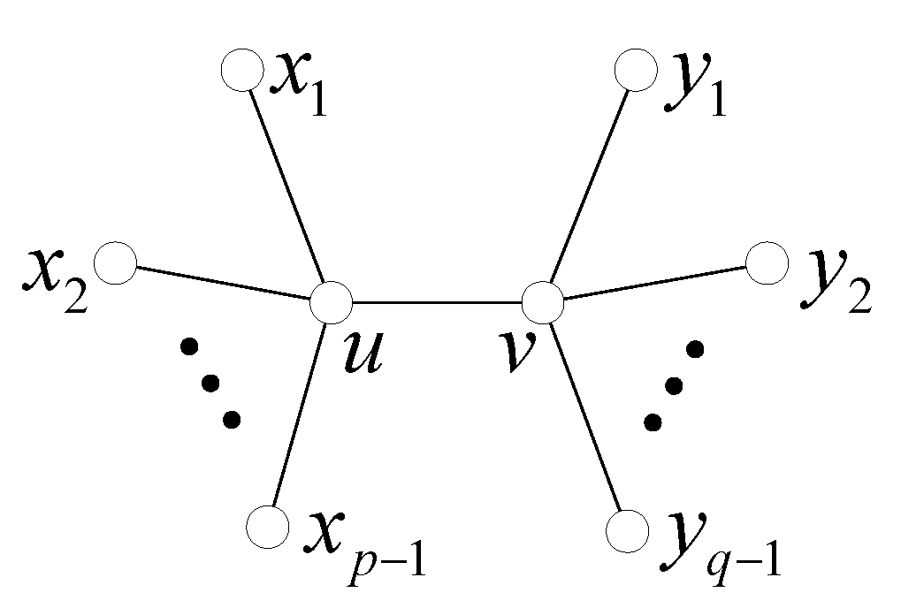
Next, we consider the bi-stars. Let $S_{p,q}$ be the bi-star with central vertices u and v, where $deg\left(u\right)=p\ge 2$ and $deg\left(v\right)=q\ge 2$. Let $X=\{x_1,x_2,\cdots ,x_{p-1}\}$ and $Y=\{y_1,y_2,\cdots ,y_{q-1}\}$. Obviously, $N\left(u\right)=X\cup \left\{v\right\}$ and $N\left(v\right)=Y\cup \left\{u\right\}$, as shown in Figure 3.

Theorem 5.

For the bi-star $S_{p,q}$ with $p+q\ge 5$, ${\chi }_{dd}\left(S_{p,q}\right)=4$.

Proof. 

Consider a proper coloring of $S_{p,q}$ in which the color classes $V_1=\left\{u\right\}$, $V_2=\left\{v\right\}$, $V_3=X$, and $V_4=Y$. Then, each vertex in the set $\left\{u\right\}\cup X$ dominates the color class $V_1$, and each vertex in the set $\left\{v\right\}\cup Y$ dominates the color class $V_2$. Moreover, the color class $V_1$ is dominated by any vertex in $V_3$, $V_2$ is dominated by any vertex in $V_4$, $V_3$ is dominated by vertex u, and $V_4$ is dominated by vertex v. Therefore, this is a domination coloring, and ${\chi }_{dd}\left(S_{p,q}\right)\le 4$.

By the Lemma 2.2 in [20], ${\chi }_d\left(S_{p,q}\right)=3$. So, $3\le {\chi }_{dd}\left(S_{p,q}\right)\le 4$. Suppose that ${\chi }_{dd}\left(S_{p,q}\right)=3$. It will be result in that each vertex in X or each vertex in y does not dominate a color class. Thus, ${\chi }_{dd}\left(S_{p,q}\right)=4$. □

Theorem 6.

Let G be a connected graph with order n. Then ${\chi }_{dd}\left(G\right)=2$ if and only if $G=K_{r,s}$ for $r,s\in \mathbf{N}$.

Proof. 

By Theorem 3 (5), if $G=K_{r,s}$, then ${\chi }_{dd}\left(G\right)=2$. We just need to prove the necessity.

Let G be a connected graph, such that ${\chi }_{dd}=2$, and $V_1$ and $V_2$ are the two color classes. If $|V_1|=1$ or $|V_2|=1$, then $G=K_{1,n-1}$. So, suppose that $|V_1|\ge 2$ and $|V_2|\ge 2$. For any vertex $x\in V_1$, since $|V_1|\ge 2$, it follows that x dominates color class $V_2$. Similarly for any vertex in $V_2$. Thus, each vertex of $V_1$ is adjacent to each vertex of $V_2$, and both $V_1$ and $V_2$ are independent. So $G=K_{r,s}$ for $r,s\in \mathbf{N}$, and the result follows. □

Theorem 7.

Let G be a connected graph with order n. Then ${\chi }_{dd}\left(G\right)=n$ if and only if $G=K_n$ for $n\in \mathbf{N}$.

Proof. 

By Theorem 3 (3), ${\chi }_{dd}\left(G\right)=n$, if $G=K_n$. We only need to prove the necessity.

Let G be a connected graph with ${\chi }_{dd}\left(G\right)=n$. Suppose that $G\ne K_n$. Thus, there exist two vertices, say x and y, such that they are not adjacent and they have a common neighbor in G. Now, we define a coloring of G in which x and y receive the same color, and each of the remaining vertices receive a unique color. This is a domination coloring, so ${\chi }_{dd}\left(G\right)\le n-1$, a contradiction. Thus, $G=K_n$, and we obtain the result. □

4. Domination Coloring in Some Classes of Graphs

In this section, we further research the domination coloring of some classes of graphs, including the split graphs, the generalized Petersen graphs $P(n,1)$, corona products, and edge corona products.

4.1. Domination Coloring for Split Graphs

We study the domination chromatic number of split graphs in this subsection.

A graph G is called a split graph if its vertex set can be partitioned into a clique and an independent set.

Theorem 8.

Let G be a split graph with split partition $(K,I)$ and its maximum clique is of order k. If there exists a dominating set D of G, such that $D\subseteq K$, and every vertex in I is adjacent to at least one vertex in $K-D$ and nonadjacent to at least one vertex in $K-D$, then ${\chi }_{dd}\left(G\right)=k$.

Proof. 

Consider a minimum domination coloring of G. Obviously, ${\chi }_{dd}\left(G\right)\ge k$. We give now a construction that yields a domination coloring of G with k colors.

First, we give to each vertex of D a unique new color from the set $\{1,\dots ,p\}$ and each vertex of $K-D$ a unique new color from the set $\{1,\dots ,q\}$, where $p+q=k$. We arrange the vertices in $K-D$ according to a circular order function defined on the set $\{1,\dots ,q\}$ as follows:

$$j\in \{1,\dots ,q\}⟹next\left(j\right)=j\mathrm{mod}\left(k\right)+1.$$

We now color the vertices of the independent set I of the split graph G. Let i be a vertex of I and let $N\left(i\right)$ be the set (of colors) of its neighbors. The color of i is given by the following formula:

$$c\left(i\right)=\min \{j:j\in \{\{1,\dots ,q\}\backslash N\left(i\right)\}\wedge next(j)\in N(i\left)\right\}.$$

Since every vertex i in I is adjacent to at least one vertex in $K-D$ and nonadjacent to at least one vertex in $K-D$, at least one color from the set $\{1,\dots ,q\}$ would be available for i. Thus, every vertex in G is properly colored. On the one hand, given that $D\subseteq K$ is a dominating set of G, each vertex dominates a color class formed by a vertex of D. On the other hand, from the above construction, each color class formed by a vertex of D is obviously dominated, and one can observe that each color j will appear only in the neighborhood of the vertex from the clique colored with the color $next\left(j\right)$. Thus, we obtain that the proposed construction gives a domination coloring for the split graph G with k colors. □

4.2. Domination Coloring for Generalized Petersen Graphs $P(n,1)$

In this subsection, we determine the domination chromatic number of the generalized Petersen graph $P(n,1)$.

Let n and k be positive integers with $n\ge 3$ and $k\le n-1$. The generalized Petersen graph $P(n,k)$ is the graph with $V\left(P(n,k)\right)=\{u_1,u_2,u_3,\cdots ,u_n\}\cup \{v_1,v_2,v_3,\cdots ,v_n\}$ and $E\left(P(n,k)\right)=\{v_i{v}_{i+1}:1\le i\le n\}\cup \{v_i{u}_i:1\le i\le n\}\cup \{u_i{u}_{i+k}:1\le i\le n\}$ where the addition in the subscript is modulo n.

The Cartesian product $G\square H$ of two graphs G and H is the graph with $V(G\square H)=V\left(G\right)\times V\left(H\right)$ and $E(G\square H)=\{(g_1,h_1)(g_2,h_2):g_1=g_2\mathrm{and}{h}_1{h}_2\in E\left(H\right)\mathrm{or}{h}_1=h_2\mathrm{and}{g}_1{g}_2\in E\left(G\right)\}$.

The generalized Petersen graph $P(n,1)$ is isomorphic to the Cartesian product $C_n\square K_2$. We now proceed to determine ${\chi }_{dd}\left(P(n,1)\right)$.

Theorem 9.

For the generalized Petersen graph $P(n,1)$, we have

$${\chi }_{dd}\left(P(n,1)\right)=\left\{\begin{array}{cc}n,\hfill & n\equiv 0\left(\mathrm{mod}4\right),\hfill \\ n+1,\hfill & otherwise.\hfill \end{array}\right.$$

Proof. 

The result is obvious when $n=3$. Now, let $n=4k+j$ where $k\ge 1$ and $0\le j\le 3$. Let $\mathcal{S}=\{N\left[v_{4i-3}\right]:1\le i\le k\}\cup \{N\left[u_{4i-1}\right]:1\le i\le k\}$. Then $\mathcal{S}$ is a family of $2k$ disjoint closed neighborhoods in $P(n,1)$. We consider the following cases:

Case 1. $j=0$.

In this case, $\mathcal{S}$ covers all the vertices of $P(n,1)$. For each closed neighborhood $N\left[x\right]$ in $\mathcal{S}$, give a color to the vertex x and another color to the neighbors of x. Obviously, $\mathcal{C}=\{\left\{v_{4i-3}\right\}:1\le i\le k\}\cup \{\left\{N\left(v_{4i-3}\right)\right\}:1\le i\le k\}\cup \{\left\{u_{4i-1}\right\}:1\le i\le k\}\cup \{\left\{N\left(u_{4i-1}\right)\right\}:1\le i\le k\}$ is a domination coloring of $P(n,1)$. Thus, ${\chi }_{dd}\left(P(n,1)\right)\le 4k=n$. On the other hand, any two disjoint closed neighborhoods in $\mathcal{S}$ cannot have a common color, which will result in some vertices having no color class to dominate, and some color classes will not dominate by any vertex. In this sense, ${\chi }_{dd}\left(P(n,1)\right)\ge 4k=n$. Therefore, ${\chi }_{dd}\left(P(n,1)\right)=4k=n$.

Case 2. $j=1$.

In this case, $\mathcal{S}$ is a collection of $2k$ disjoint closed neighborhoods in $P(n,1)$ and the vertices $v_{n-1}$ and $u_n$ are not covered by $\mathcal{S}$. Similar to Case 1, give two colors to each closed neighborhood in $\mathcal{S}$ and two new colors to $v_{n-1}$ and $u_n$. Then, $\mathcal{C}=\{\left\{v_{4i-3}\right\}:1\le i\le k\}\cup \{\left\{N\left(v_{4i-3}\right)\right\}:1\le i\le k\}\cup \{\left\{u_{4i-1}\right\}:1\le i\le k\}\cup \{\left\{N\left(u_{4i-1}\right)\right\}:1\le i\le k\}\cup \left\{v_{n-1}\right\}\cup \left\{u_n\right\}$ is a domination coloring of $P(n,1)$. Thus, ${\chi }_{dd}\left(P(n,1)\right)\le 4k+2=n+1$. On the other hand, to ensure that every vertex dominate a color class and every color class is dominated by a vertex, the vertices $v_{n-1}$ and $u_n$ should be colored uniquely, respectively. Hence, ${\chi }_{dd}\left(P(n,1)\right)\ge 4k+2=n+1$. Therefore, ${\chi }_{dd}\left(P(n,1)\right)=4k+2=n+1$.

Case 3. $j=2$.

In this case, $\mathcal{S}$ is a collection of $2k$ disjoint closed neighborhoods in $P(n,1)$ and the vertices $v_{n-2}$, $v_{n-1}$, $u_{n-1}$ and $u_n$ are not covered by $\mathcal{S}$. $\mathcal{C}=\{\left\{v_{4i-3}\right\}:1\le i\le k\}\cup \{\left\{N\left(v_{4i-3}\right)\right\}:1\le i\le k\}\cup \{\left\{u_{4i-1}\right\}:1\le i\le k\}\cup \{\left\{N\left(u_{4i-1}\right)\right\}:1\le i\le k\}\cup \{v_{n-2},u_{n-1}\}\cup \left\{v_{n-1}\right\}\cup \left\{u_n\right\}$ is a domination coloring of $P(n,1)$. Thus, ${\chi }_{dd}\left(P(n,1)\right)\le 4k+3=n+1$. On the other hand, to ensure the domination properties, the vertices $v_{n-2}$, $v_{n-1}$, $u_{n-1}$ and $u_n$ need at least three new colors. Hence, ${\chi }_{dd}\left(P(n,1)\right)\ge 4k+3=n+1$. Therefore, ${\chi }_{dd}\left(P(n,1)\right)=4k+3=n+1$.

Case 4. $j=3$.

In this case, $\mathcal{S}\cup N\left[v_{4k+1}\right]$ is a collection of $2k+1$ disjoint closed neighborhoods in $P(n,1)$ and the vertices $u_{n-1}$ and $u_n$ are not covered by these neighborhoods. Then $\mathcal{C}=\{\left\{v_{4i-3}\right\}:1\le i\le k\}\cup \{\left\{N\left(v_{4i-3}\right)\right\}:1\le i\le k\}\cup \{\left\{u_{4i-1}\right\}:1\le i\le k\}\cup \{\left\{N\left(u_{4i-1}\right)\right\}:1\le i\le k\}\cup \left\{v_{4k+1}\right\}\cup \left\{N\left(v_{4k+1}\right)\right\}\cup \left\{u_{n-1}\right\}\cup \left\{u_n\right\}$ is a domination coloring of $P(n,1)$. Thus, ${\chi }_{dd}\left(P(n,1)\right)\le 4k+4=n+1$. Similar to the above analysis, ${\chi }_{dd}\left(P(n,1)\right)\ge 4k+4=n+1$. Therefore, ${\chi }_{dd}\left(P(n,1)\right)=4k+4=n+1$.

Thus, the result follows. □

4.3. Domination Coloring for Corona Products

For graphs G and H, the corona product $G\circ H$ is obtained from one copy of G and $n\left(G\right)$ copies of H by joining with an edge each vertex of the ith copy of H, $i\in \left[n\right(G\left)\right]$, to the ith vertex of G. If $v\in V\left(G\right)$, then the copy of H in $G\circ H$ corresponding to v will be denoted by $H_v$. We may consider the vertex set of $G\circ H$ to be

$$V(G\circ H)=V\left(G\right)\cup \left(\bigcup _{v\in V\left(G\right)}V\left(H_v\right)\right).$$

The dominator and dominated chromatic numbers of corona products are already known.

Theorem 10

([36]). If G and H are graphs, then ${\chi }_d(G\circ H)=n\left(G\right)+\chi \left(H\right)$.

Theorem 11

([33]). If G and H are graphs, then ${\chi }_{dom}(G\circ H)=n\left(G\right)\chi \left(H\right)$.

We now give a general result for the domination chromatic number of corona products.

Theorem 12.

If G and H are graphs, then ${\chi }_{dd}(G\circ H)\le n\left(G\right)(\chi \left(H\right)+1)$.

Proof. 

Set $n=n\left(G\right)$ and color $G\circ H$ as follows. First, we color each vertex of $V\left(G\right)$ an unique color. Second, we properly color every copy of H with $\chi \left(H\right)$ distinct colors. Clearly, the obtained coloring is a domination coloring of $G\circ H$. Indeed, each vertex $v\in V\left(G\right)$ forms a color class of cardinality 1 and the color class $\left\{v\right\}$ is dominated by any adjacent vertices of v, while each vertex from $H_v$ is adjacent to the vertex v and dominate the color class $\left\{v\right\}$, the color class formed by vertices in $H_v$ is dominated by the corresponding vertex v. Therefore, ${\chi }_{dd}(G\circ H)\le n\left(G\right)(\chi \left(H\right)+1)$. □

4.4. Domination Coloring for Edge Corona Products

For graphs G and H, the edge corona $G\diamond H$ is obtained by taking one copy of G and $m\left(G\right)$ disjoint copies of H one-to-one assigned to the edges of G, and for every edge $v{v}^{\prime }\in E\left(G\right)$ joining v and $v^{\prime }$ to every vertex of the copy of H associated to $v{v}^{\prime }$. If $e=v{v}^{\prime }\in E\left(G\right)$, then the copy of H in $G\diamond H$ corresponding to $v{v}^{\prime }$ will be denoted with $H_{v{v}^{\prime }}$ (or simply $H_e$). Hence we may consider the vertex set of $G\diamond H$ to be

$$V(G\diamond H)=V\left(G\right)\cup \left(\bigcup _{v{v}^{\prime }\in E\left(G\right)}V\left(H_{v{v}^{\prime }}\right)\right).$$

The dominator and dominated chromatic numbers of edge corona products have been studied, which were related to the matching number ${\alpha }^{\prime }$ and the vertex cover number $\beta$.

Theorem 13

([36]). If G and H are graphs, then ${\chi }_d(G\diamond H)=\beta \left(G\right)+\chi \left(H\right)+1$.

Theorem 14

([36]). If G is a graph without pendant vertices, then ${\chi }_{dom}(G\diamond H)\ge {\alpha }^{\prime }\left(G\right)\chi \left(H\right)+{\chi }_{dom}\left(G\right)$.

Theorem 15

([36]). If G has k pendant vertices, then ${\chi }_{dom}(G\diamond H)\ge {\alpha }^{\prime }\left(G\right)\chi \left(H\right)+k$.

Theorem 16

([36]). If G and H are graphs, then ${\chi }_{dom}(G\diamond H)\le \beta \left(G\right)\chi \left(H\right)+{\chi }_{dom}\left(G\right)$, with equality when G is bipartite graph without pendant vertices.

In the following, we give a general result for the domination chromatic number of edge corona products.

Theorem 17.

If G and H are graphs, then ${\chi }_{dd}(G\diamond H)\le \beta \left(G\right)(\chi \left(H\right)+2)$.

Proof. 

Let $K=\{v_1,\cdots ,v_{\beta \left(G\right)}\}$ be a minimum vertex cover of G, so that $\left|K\right|=\beta \left(G\right)$. Partition $E\left(G\right)$ into subsets of edges $E_1,\cdots ,E_{\beta \left(G\right)}$, such that if $e\in E_i$, then $v_i$ is an endpoint of e, $i=1,\cdots ,\beta \left(G\right)$. Partition $V-K$ into subsets of vertices $V_1,\cdots ,V_{\beta \left(G\right)}$, such that if $u\in V_i$, then $u{v}_i\in E_i$, $i=1,\cdots ,\beta \left(G\right)$. It is clear that such partitions always exists since K is a vertex cover. Notice that each $V_i$ is a independent set, $i=1,\cdots ,\beta \left(G\right)$.

Now, define a coloring c of $G\diamond H$ as follows. First, for each set of edges $E_i$, reserve private $\chi \left(H\right)$ colors and color with each of the corresponding subgraphs $H_e$, $e\in E_i$. Second, color the vertices of K with $\beta \left(G\right)$ colors. Third, color the vertices of $V_1,\cdots ,V_{\beta \left(G\right)}$ with additional $\beta \left(G\right)$ colors. Then, c is the domination coloring of $G\diamond H$. Indeed, each vertex in each $H_e$ dominate a corresponding color class $\left\{v_i\right\}$, and the color classes of those copies of H with common $\chi \left(H\right)$ colors are dominated by the corresponding vertex $v_i$. For each vertex $v_i$ in K, there exist color classes dominated by $v_i$. Moreover, the color class $\left\{v_i\right\}$ can be dominated by any adjacent vertex of $v_i$. Moreover, each vertex in $V_i$ dominates the color class $\left\{v_i\right\}$, and the color class $V_i$ is dominated by vertex $v_i$. Hence, ${\chi }_{dd}(G\diamond H)\le \beta \left(G\right)(\chi \left(H\right)+2)$. □

5. Graphs with ${\mathbf{\chi }}_{\mathbf{dd}}\left(\mathbf{G}\right)=\mathbf{\chi }\left(\mathbf{G}\right)$

For any graph G, we have ${\chi }_{dd}\left(G\right)\ge \chi \left(G\right)$. In this section, we investigate graphs for which ${\chi }_{dd}\left(G\right)=\chi \left(G\right)$.

The following theorem directly follows from Proposition 1.

Theorem 18.

Let G be a connected graph, if $\gamma \left(G\right)=1$, then ${\chi }_{dd}\left(G\right)=\chi \left(G\right)$.

A unicyclic graph is a graph that contains only one cycle. In the following, we characterize unicyclic graphs with ${\chi }_{dd}=\chi$.

Theorem 19.

Let G be a connected unicyclic graph. Then ${\chi }_{dd}\left(G\right)=\chi \left(G\right)$ if and only if G is isomorphic to $C_3$ or $C_4$ or $C_5$ or the graph obtained from $C_3$ by attaching any number of leaves at one vertex of $C_3$.

Proof. 

For the sufficiency, the result is obvious if G is the graph meet conditions. We consider only the necessity. Let G be a connected unicyclic graph with ${\chi }_{dd}\left(G\right)=\chi \left(G\right)$, and C the unique cycle of G.

Case 1. If C is an even cycle, then $\chi \left(G\right)=2$ and ${\chi }_{dd}\left(G\right)=2$. It follows that G cannot contain any other vertices not on C, otherwise ${\chi }_{dd}\left(G\right)\ge 3$. By Theorem 3(2), $G=C_4$.

Case 2. If C is an odd cycle, then ${\chi }_{dd}\left(G\right)=\chi \left(G\right)=3$. Suppose there exists a support vertex x not on C. Since x or the leaf is a color class in each ${\chi }_{dd}$-coloring of G, it follows that ${\chi }_{dd}\left(G\right)\ge 4$, which is a contradiction. Hence, all of the support vertices lie on C, and any vertex not on C is a leaf. Moreover, the number of support vertices is at most one. Otherwise, it follows that some color classes are not dominated, since there exists some ${\chi }_{dd}$-coloring of G in which every support vertex appears as a singleton color class.

Case 2.1. If $\left|C\right|=3$, then G is isomorphic to $C_3$ or the graph obtained from $C_3$ by attaching any number of leaves at exactly one vertex of $C_3$.

Case 2.2. Suppose that $\left|C\right|\ge 5$. If there exists a support vertex x on C, then there exists a ${\chi }_{dd}$-coloring $\{V_1,V_2,\left\{x\right\}\}$ of G, such that $V_1$ contains all of the leaves of x. Now, we get two vertices u and v on C, such that $u\in V_1,v\in V_2$, both u and v are not adjacent to x. Clearly, v does not dominate any color class and the color class $V_1$ is not dominated by any vertex, which is a contradiction. Thus, G has no support vertices and $G=C$. By Theorem 3(2), $G=C_5$. So, the theorem follows. □

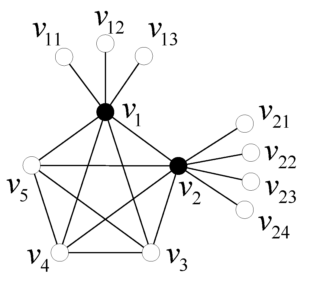
For the complete graph $K_n$, we know that ${\chi }_{dd}\left(K_n\right)=\chi \left(K_n\right)=n$. Next, we construct a family of graphs by attaching leaves at some vertices of the complete graph. We denote by ${\mathcal{K}}_n^m$ the family of graphs obtained by attaching leaves at m vertices of $K_n$, $1\le m\le n$. We take no account of the number of leaves attached at any vertex in the notation, since it does not impact the domination chromatic number. Moreover, we denote any element in ${\mathcal{K}}_n^m$ by $K_n^m$. For example, a instance of $K_5^2$ is shown in Figure 4.

Theorem 20.

For $m\le \lfloor \frac{n}{2}\rfloor$, ${\chi }_{dd}\left(K_n^m\right)=\chi \left(K_n^m\right)$.

Proof. 

For any $1\le m\le n$, $K_n^m$ is n-colorable. So, $\chi \left(K_n^m\right)=n$. Next, we consider a domination coloring of $K_n^m$. On the one hand, vertex-attached leaves should be partitioned into a singleton color class, since each leaf has to dominate a color class formed by its only neighbor. On the other hand, leaves attached to different vertices have to be partitioned into different color classes, otherwise, there exists no vertex dominating the color class. Thus, at most $\lfloor \frac{n}{2}\rfloor$ vertices can be attached to leaves of $K_n$, in order to guarantee that $K_n^m$ is n-domination colorable. The result follows. □

6. Conclusions

In this paper, we introduce the concept of domination coloring where both vertices and color classes should satisfy the domination property. Moreover, an application of domination coloring in a social network scenario is presented. We prove the k-domination coloring problem is NP-complete by a reduction from the k-coloring problem. We provide basic results and properties of the domination chromatic number ${\chi }_{dd}\left(G\right)$, and further research ${\chi }_{dd}\left(G\right)$ of the split graphs, the generalized Petersen graphs $P(n,1)$, the corona products, and edge corona products. In particular, we establish a relationship between the domination chromatic number and other graph parameters, such as the matching number, the vertex cover number, and the clique number. Moreover, we provide sufficient and necessary conditions for connected unicyclic graphs with ${\chi }_{dd}=\chi$, and construct a class of graphs with ${\chi }_{dd}=\chi$. Our future work will focus on the relationships among the domination chromatic number, the domination number, and the chromatic number, and discuss graphs with ${\chi }_{dd}=\chi$, ${\chi }_{dd}=\gamma$, ${\chi }_{dd}=\chi ·\gamma$. Moreover, we will explore the application of domination coloring in practice.

References

- Franklin, P. The four color problem. Am. J. Math. 1922, 44, 225–236. [Google Scholar] [CrossRef]
- Appel, K.; Haken, W. Every planar map is four colorable. part i: Discharging. Ill. J. Math. 1977, 21, 429–490. [Google Scholar] [CrossRef]
- Appel, K.; Haken, W.; Koch, J. Every planar map is four colorable. part ii: Reducibility. Ill. J. Math. 1977, 21, 491–567. [Google Scholar] [CrossRef]
- Pardalos, P.M.; Mavridou, T.; Xue, J. The Graph Coloring Problem: A Bibliographic Survey; Springer: Boston, MA, USA, 1998. [Google Scholar]
- Malaguti, E.; Toth, P. A survey on vertex coloring problems. Int. Trans. Oper. Res. 2010, 17, 1–34. [Google Scholar] [CrossRef]
- Borodin, O.V. Colorings of plane graphs: A survey. Discret. Math. 2013, 313, 517–539. [Google Scholar] [CrossRef]
- Li, G.Z.; Simha, R. The partition coloring problem and its application to wavelength routing and assignment. In Proceedings of the First Workshop on Optical Networks, Dallas, TX, USA; 1 May 2000; pp. 1–19.
- Zhu, E.Q.; Jiang, F.; Liu, C.J.; Xu, J. Partition independent set and reduction-based approach for partition coloring problem. IEEE Trans. Cybern. 2020, 1–10. [Google Scholar] [CrossRef] [PubMed]
- MacGillivray, G.; Seyffarth, K. Domination numbers of planar graphs. J. Graph Theory 1996, 22, 213–229. [Google Scholar] [CrossRef]
- Haynes, T.W.; Hedetniemi, S.T.; Slater, P.J. Fundamentals of Domination in Graphs; Marcel Dekker, Inc.: New York, NY, USA, 1998. [Google Scholar]
- Haynes, T.W.; Hedetniemi, S.T.; Slater, P.J. Domination in Graphs: Volume 2: Advanced Topics; Marcel Dekker, Inc.: New York, NY, USA, 1998. [Google Scholar]
- Honjo, T.; Kawarabayashi, K.-I.; Nakamoto, A. Dominating sets in triangulations on surfaces. J. Graph Theory 2010, 63, 17–30. [Google Scholar] [CrossRef]
- King, E.L.; Pelsmajer, M.J. Dominating sets in plane triangulations. Discret. Math. 2010, 310, 2221–2230. [Google Scholar] [CrossRef] [Green Version]
- Ananchuen, N.; Ananchuen, W.; Plummer, M.D. Domination in Graphs; Birkhauser: Boston, MA, USA, 2011. [Google Scholar]
- Campos, C.N.; Wakabayashi, Y. On dominating sets of maximal outerplanar graphs. Discret. Appl. Math. 2013, 161, 330–335. [Google Scholar] [CrossRef] [Green Version]
- Li, Z.P.; Zhu, E.Q.; Shao, Z.H.; Xu, J. On dominating sets of maximal outerplanar and planar graphs. Discret. Appl. Math. 2016, 198, 164–169. [Google Scholar] [CrossRef]
- Liu, C.J. A note on domination number in maximal outerplanar graphs. Discret. Appl. Math. 2021, 293, 90–94. [Google Scholar] [CrossRef]
- Chellali, M.; Volkmann, L. Relations between the lower domination parameters and the chromatic number of a graph. Discret. Math. 2004, 274, 1–8. [Google Scholar] [CrossRef]
- Hedetniemi, S.M.; Hedetniemi, S.T.; Laskar, R.; Mcrae, A.A.; Wallis, C.K. Dominator partitions of graphs. J. Comb. Inf. Syst. Sci. 2009, 34, 183–192. [Google Scholar]
- Gera, R.M.; Rasmussen, C.; Horton, S. Dominator colorings and safe clique partitions. Congr. Numer. 2006, 181, 19–32. [Google Scholar]
- Gera, R.M. On dominator colorings in graphs. Graph Theory Notes N. Y. 2007, 52, 25–30. [Google Scholar]
- Gera, R.M. On the dominator colorings in bipartite graphs. In Proceedings of the 4th International Conference on Information Technology, New Generations, Las Vegas, NV, USA, 2–4 April 2007; pp. 947–952. [Google Scholar]
- Kavitha, K.; David, N.G. Dominator coloring of some classes of graphs. Int. J. Math. Arch. 2012, 3, 3954–3957. [Google Scholar]
- Chellali, M.; Maffray, F. Dominator colorings in some classes of graphs. Graphs Comb. 2012, 28, 97–107. [Google Scholar] [CrossRef]
- Merouane, H.B.; Chellali, M. On the dominator colorings in trees. Discuss. Math. Graph Theory 2012, 32, 677–683. [Google Scholar]
- Arumugam, S.; Bagga, J.; Chandrasekar, K.R. On dominator colorings in graphs. Proc. Math. Sci. 2012, 122, 561–571. [Google Scholar] [CrossRef]
- Kazemi, A.P. Total dominator chromatic number of a graph. Trans. Comb. 2015, 4, 57–68. [Google Scholar]
- Kazemi, A.P. Total dominator coloring in product graphs. Util. Math. 2014, 94, 329–345. [Google Scholar]
- Kazemi, A.P. Total dominator chromatic number and Mycieleskian graphs. Util. Math. 2017, 103, 129–137. [Google Scholar]
- Henning, M.A. Total dominator colorings and total domination in graphs. Graphs Comb. 2015, 31, 953–974. [Google Scholar] [CrossRef]
- Merouane, H.B.; Haddad, M.; Chellali, M.; Kheddouci, H. Dominated colorings of graphs. Graphs Comb. 2015, 31, 713–727. [Google Scholar] [CrossRef]
- Guillaume, B.; Houcine, B.M.; Mohammed, H.; Hamamache, K. On some domination colorings of graphs. Discret. Appl. Math. 2017, 230, 34–50. [Google Scholar]
- Choopani, F.; Jafarzadeh, A.; Erfanian, A.; Mojdeh, D.A. On dominated coloring of graphs and some nordhaus–gaddum-type relations. Turk. J. Math. 2018, 42, 2148–2156. [Google Scholar] [CrossRef]
- Krithika, R.; Rai, A.; Saurabh, S.; Tale, P. Parameterized and exact algorithms for class domination coloring. Discret. Appl. Math. 2021, 291, 286–299. [Google Scholar] [CrossRef]
- Bondy, J.A.; Murty, U.S.R. Graph Theory with Applications; MacMillan: London, UK, 1976. [Google Scholar]
- Klavar, S.; Tavakoli, M. Dominated and dominator colorings over (edge) corona and hierarchical products. Appl. Math. Comput. 2021, 390, 1–7. [Google Scholar] [CrossRef]
Figure 1.
The graphs G and .
Figure 2.
The Petersen graph.
Figure 3.
The bi-star .
Figure 4.
A instance of .
Publisher’s Note: MDPI stays neutral with regard to jurisdictional claims in published maps and institutional affiliations. |
© 2022 by the authors. Licensee MDPI, Basel, Switzerland. This article is an open access article distributed under the terms and conditions of the Creative Commons Attribution (CC BY) license (https://creativecommons.org/licenses/by/4.0/).
Share and Cite
MDPI and ACS Style
Zhou, Y.; Zhao, D.; Ma, M.; Xu, J. Domination Coloring of Graphs. Mathematics 2022, 10, 998. https://doi.org/10.3390/math10060998
AMA Style
Zhou Y, Zhao D, Ma M, Xu J. Domination Coloring of Graphs. Mathematics. 2022; 10(6):998. https://doi.org/10.3390/math10060998
Chicago/Turabian StyleZhou, Yangyang, Dongyang Zhao, Mingyuan Ma, and Jin Xu. 2022. "Domination Coloring of Graphs" Mathematics 10, no. 6: 998. https://doi.org/10.3390/math10060998
Note that from the first issue of 2016, this journal uses article numbers instead of page numbers. See further details here.