
Unsupervised and Supervised Methods to Estimate Temporal-Aware Contradictions in Online Course Reviews


Department of Computer Science, Aix Marseille Université, CNRS, LIS, 13007 Marseille, France
*
Author to whom correspondence should be addressed.
Mathematics 2022, 10(5), 809; https://doi.org/10.3390/math10050809
Submission received: 13 December 2021
/
Revised: 19 February 2022
/
Accepted: 25 February 2022
/
Published: 3 March 2022
(This article belongs to the Special Issue Natural Language Processing (NLP) and Machine Learning (ML)—Theory and Applications)
Abstract
:The analysis of user-generated content on the Internet has become increasingly popular for a wide variety of applications. One particular type of content is represented by the user reviews for programs, multimedia, products, and so on. Investigating the opinion contained by reviews may help in following the evolution of the reviewed items and thus in improving their quality. Detecting contradictory opinions in reviews is crucial when evaluating the quality of the respective resource. This article aims to estimate the contradiction intensity (strength) in the context of online courses (MOOC). This estimation was based on review ratings and on sentiment polarity in the comments, with respect to specific aspects, such as “lecturer”, “presentation”, etc. Between course sessions, users stop reviewing, and also, the course contents may evolve. Thus, the reviews are time dependent, and this is why they should be considered grouped by the course sessions. Having this in mind, the contribution of this paper is threefold: (a) defining the notion of subjective contradiction around specific aspects and then estimating its intensity based on sentiment polarity, review ratings, and temporality; (b) developing a dataset to evaluate the contradiction intensity measure, which was annotated based on a user study; (c) comparing our unsupervised method with supervised methods with automatic feature selection, over the dataset. The dataset collected from coursera.org is in English. It includes 2244 courses and 73,873 user-generated reviews of those courses.The results proved that the standard deviation of the ratings, the standard deviation of the polarities, and the number of reviews are suitable features for predicting the contradiction intensity classes. Among the supervised methods, the J48 decision trees algorithm yielded the best performance, compared to the naive Bayes model and the SVM model.
Keywords:
sentiment analysis; aspect detection; temporality; rating; feature evaluation; contradiction intensityMSC:
68T501. Introduction
Since the evolution of the Internet, and more specifically of the Web 2.0, where users also represent content producers, it has become essential to be able to analyze the associated textual information in order to facilitate better navigation through it. In particular, Internet users massively post comments about the content they watch or the products they buy. However, it is often quite difficult to find one’s way through these comments, partly because of their quantity, but also because of the way they are written. It thus becomes essential to carry out automatic processing [1,2,3].
It often happens for various aspects of a product or content to be discussed in the comments, so in order to have a better idea of the product or content, it is necessary to extract and compare the comments about these same aspects. Moreover, the very quantity of comments concerning the same aspect is often important, and the opinions can be very divergent. The idea of this article was to extract the opinions by aspect, to detect if there was a contradiction among the opinions on the same aspect, and then to measure the intensity of this contradiction. This measure, then, allows the user reading the reviews to have a metric indicating if the reviews are all (or almost all) in the same direction, positive or negative, or if there is a large divergence of opinion on a specific aspect. The measure then indicates that it is difficult to tell if this aspect is rated positively or negatively. This measure enabled us to alert the user by indicating the points of disagreement present in the comments for particular aspects, thus highlighting the aspects for which the point of view is the most subjective to each person’s appreciation. Table 1 shows an example of contradictory comments from an online course, concerning the “Lesson”.
In order to measure the intensity of the contradictions in the comments, it is first necessary to extract the aspects [4,5] from them and to measure the sentiments [6] expressed around these aspects. We therefore focused in this article only on the contradictions expressed through the subjectivity present in the comments. We did not deal with contradictions based on facts.
The contributions of this paper are the following:
- (C1). In this paper, we give the definition of the subjective contradiction occurring in reviews, around aspects. Four research questions were raised by this definition:
- –
- RQ1: How do we define the notion of subjective contradiction around an aspect? The definition of the notion of subjective contradiction is based on the notion of sentiment diversity with respect to aspects. We considered, in this article, the notion of diversity as the dispersion of sentiments (sentiment polarity);
- –
- RQ2: How can the strength (intensity) of a contradiction occurring in reviews be estimated? This was performed by computing the degree of dispersion of sentiment polarity around an aspect of a web resource;
- –
- RQ3: How do we balance the sentiment polarity around an aspect and the global rating of a review leading to the underlying question, when computing the intensity of a contradiction? What is the weight of the global rating of a review in the expression of feelings around an aspect?
- –
- RQ4: Freshness and temporality are essential in Web 2.0; it is therefore necessary to take into account the temporality of the reviews when computing contradiction intensity;
- (C2). We present the development of a data collection that allows the evaluation of the contradiction intensity estimation. The evaluation was based on a user study;
- (C3). We performed an experimental comparison, over our corpus, of the unsupervised method based on our definition of subjective contradiction with supervised methods with automatic feature selection.
To the best of our knowledge, no other model has tried to measure the contradiction’s intensity for subjective elements. Thus, it was not possible for us to use specialized state-of-the-art models.
The paper is organized as follows. Section 2 of our paper presents the background and related work. The third section presents the learning model and the non-learning model that we used as a baseline. The fourth section presents our test dataset and the experiments and discussions around the results. The article ends with the conclusion Section.
2. Background and Related Work
The use of several state-of-the-art methods is necessary in order to establish a process as complex as contradiction detection. Moreover, very few—if any—studies deal with the detection and measurement of intensity in explicitly subjective sentences. This section presents some of the approaches needed for such detection and measurement, as well as related work such as fact-based contradiction detection, controversy detection, point-of-view detection, disagreement detection, and position detection.
2.1. Contradiction Detection Approaches
Our work was focused on detecting and assessing the level of subjective contradiction on a particular aspect in the comments. In the literature, some topics are related and relatively close to our work. Examples include work on fact contradiction, the detection and evaluation of controversies, disputes, scandals, the detection of viewpoints, and vandalized pages, mainly in Wikipedia.
One of the research interests that is closest to the present work is given by factual contradiction. The research of [7,8,9,10] is representative of this type of study. At present, there are two approaches that see contradictions as a type of textual inference (for instance, entailment identification) and whose analyses are based on the use of linguistic methods. In some works, such as those of Harabagiu et al. [7], the authors proposed to use linguistic features specific to this kind of problem, such as semantic information, for instance negations (for example: “I hate you”—“I don’t hate you”) or antonymy (i.e., words with opposite meanings—“light” vs. “dark” or “hot” vs. “cold”). Two mutually exclusive sentences, on the same topic, are then seen as a textual implication expressing a contradiction. In a similar way, in the work of [8], seven types of features (e.g., antonymy, negation, numeric mismatches) can be seen as contributing to a contradiction. These feature types can then lead to incorrect data (“The Eiffel Tower is 421 m high—The Eiffel Tower is 321 m high). The authors then define a contradiction as two sentences that cannot be true simultaneously. This definition cannot be applied to our case because we dealt with subjective expressions and not with factual data. A scalable and automatic solution to contradiction detection was also proposed by Tsytsarau et al. [9,10]. The solution considered by the authors was to aggregate the sentiment scores determined for the sentences and infer whether there is a contradiction or not. When the diversity in terms of sentiment is high, but the aggregation of the sentiment score tends towards zero, then there is a contradiction. However, the authors only sought to detect the presence or absence of a contradiction and not to evaluate its level. Fact contradictions may be studied with respect to a specific field, such as medicine [11]. In this paper, we focused on course reviews from an online platform. The contradiction we targeted concerns several reviews, for the same online course and for the same period (course session); thus, it may be characterized as extrinsic relative to one review in particular. Other research focused on intrinsic contradiction detection, for instance detecting self-contradicting articles from Wikipedia [12].
Our corpus is in English. However, there are works that have tackled contradictions in other languages, such as Spanish [13], Persian [14], or German [15]. The development of multilingual models can also be considered, as is already the case in the analysis of sentiments and emotions [16,17].
Another research topic, very close to ours, concerns controversy detection. The concepts of controversy and dispute are relatively similar, except that a controversy involves a large group of people who have strong disagreements about a particular issue. Indeed, the Merriam-Webster dictionary definition for controversy states: “argument that involves many people who strongly disagree about something, strong disagreement about something among a large group of people”. A similar definition was given in [18,19], but with a temporal nuance: a controversy is usually defined as a discussion regarding a specific target entity, which provokes opposing opinions among people, for a finite duration of time. In the majority of works on controversies, the aim is to usually discover the subject of the controversy and not to quantify it or to find the level of virulence of the exchanges. Discovering the subject of the controversy is then often seen as a problem of classification aiming to find out which documents, paragraphs, or sentences are controversial and which are not or to discover the subject itself. Balasubramanyan et al. [20] used a semi-supervised latent variable model to detect the topics and the degree of polarization these topics caused. Dori-Hacohen and Allan [21,22] treated the problem as a binary classification: whether the web page has a controversial topic or not. To perform this classification, the authors looked for Wikipedia pages that corresponded to the given web page, but displayed a degree of controversy. Garimella et al. [23] constructed a conversation graph on a topic, then partitioned the conversation graph to identify potential points of controversy, and measured the controversy’s level based on the characteristics of the graph. Guerra et al. [24] constructed a metric based on the analysis of the boundary in a graph between two communities. The metric was applied to the analysis of communities on Twitter by constructing graphs from retweets. Jang and Allan [25] constructed a controversial language model based on DBpedia. Lin and Hauptmann [26] proposed to measure the proportion, if any, by which two collections of documents were different. In order to quantify this proportion, they used a measure based on statistical distribution divergence. Popescu and Pennacchiotti [19] proposed to detect controversies on Twitter. Three different models were suggested. They were all based on supervised learning using linear regression. Sriteja et al. [27] performed an analysis of the reaction of social media users to press articles dealing with controversial issues. In particular, they used sentiment analysis and word matching to accomplish this task. Other works sought to quantify controversies. For instance, Morales et al. [28] quantified polarity via the propagation of opinions of influential users on Twitter. Garimella et al. [29] proposed the use of a graph-based measure by measuring the level of separation of communities within the graph.
Quite close to our work is the concept of “point of view“, also known in the literature as the notion of “collective opinions”, where a collective opinion is the set of ideas shared by a group. There is also a proximity with the work on the notion of controversy, but with generally less opposition in the case of “points of view” than in that of “controversy”. In a sense, the notion of points of view can also be seen as a controversy on a smaller scale. Among the significant works on the concept of “points of view” is [30], which used the multi-view Latent Dirichlet Allocation (LDA) model. In addition to topic modeling at the word level, as LDA performs, the model uses a variable that gives the point of view at the document level. This model was applied to the discovery of points of view in essays. Cohen and Ruths [31] developed a supervised-learning-based system for point of view detection in social media. The approach treats viewpoint detection as a classification problem. The model used to perform this task was an SVM. Similarly, Conover et al. [32] developed a system based on SVM and took into account social interactions in social networks in order to classify viewpoints. Paul and Girju [33] used the Topic-Aspect Model (TAM) by hijacking the model using aspects as viewpoints. The authors of [34] used an unsupervised approach inspired by LDA, based on Dirichlet distributions and discrete variables, to identify the users’ point of view. Trabelsi and Zaïane [35] used the Joint Topic Viewpoint (JTV) model, which jointly models themes and viewpoints. JTV defines themes and viewpoint assignments at the word level and viewpoint distributions at the document level. JTV considers all words as opinion words, without distinguishing between opinion words and topic words. Thonet et al. [36] presented VODUM, an unsupervised topic model designed to jointly discover viewpoints, topics, and opinions in text.
A line of research that is also relatively similar to our work, even if it does not always involve the notion of subjectivity, is the problem of detecting expressions of restraint or the problem of detecting disagreement. This problem has been widely addressed in the literature. In particular, Galley et al. [37] used a maximum entropy classifier. They first identified adjacent pairs using a classification based on maximum entropy from a set of lexical, temporal, and structural characteristics. They then ranked these pairs as agreement or disagreement. Menini and Tonelli [38] used an SVM. They also used different characteristics based on the feelings expressed in the text (negative or positive). They also used semantic features (word embeddings, cosine similarity, and entailment). Mukherjee and Liu [39] adopted a semi-supervised approach to identify expressions of contention in discussion forums.
Another quite close research is the one concerning position detection. Position (stance) detection is a classification problem where the position of the author of the text is obtained in the form of a category label of this set: favorable, against, neither. Among the works on the notion of “stance”, Mohammad et al. [40,41] used an SVM and relatively simple features based on N-grams of words and characters. In [42], the authors used a bi-Long Short-Term Memory (LSTM) in order to detect the position of the author of the text. The input of their model was a word embedding based on Word2Vec. Gottopati et al. [43] used an unsupervised approach to detect the position of an author. In order to perform this task, they used a template based on collapsed Gibbs sampling. Johnson and Goldwasser [44] used a weakly supervised method to extract the way questions are formulated and to extract the temporal activity patterns of politicians on Twitter. Their method was applied to the tweets of popular politicians and issues related to the 2016 election. Qiu et al. [34,45] used a regression-based latent factor model, which jointly models user arguments, interactions, and attributes. Somasundaran and Wiebe [46] used an SVM employing characteristics based on feelings and argumentation of opinions, as well as targets of feelings and argumentation. For more details on this topic, refer to [47].
Our work is relatively close to the detection and analysis of points of view, with however some differences. We focused on opposing points of view. Indeed, our subject of study relates to the subjective oppositions expressed by several individuals. It is this subjective opposition, with the formulation of an opinion using feelings, which we call “contradiction” within the article, that we tried to capture. Our work can also be considered close to the work on stance since we looked at oppositions. However, the observed oppositions were not the same since they were not favorable or unfavorable of an assertion, but rather positive or negative about an aspect. The main difference is yet again in the strong expression of subjectivity, which may be absent in the expression of stance. We did not consider our work as being exactly in the domain of controversies since there was no constructed argumentation. Indeed, we considered in our research reviews that were independent of each other, and we were not in the case of a discussion as in a forum, for example. Moreover, unlike most other authors, we did not only try to find out if there was a contradiction among several individuals. We measured the strength of this contradiction in order to obtain a level in the contradiction evaluation.
2.2. Methods for Aspect Detection
One of the first steps to be taken in order to detect and evaluate the intensity of a contradiction is to extract the necessary aspects. For this purpose, several methods are available. One of the first developed methods [48] used a frequent equational-sentences-based method, which represents a common information extraction technique. These approaches are relatively efficient and simple to implement, especially when the aspects are composed of a single word with a high frequency, but decrease in performance when the frequency of the aspects is relatively low. Other approaches, very widespread in the extraction of aspects, are, for example, the use of Conditional Random Fields (CRFs) or the use of Hidden Markov Models (HMMs) [49]. Other methods, unsupervised, are also often used in this task. For instance, Reference [50] developed a model based on the multi-grain topic model. In [4], the use of unsupervised Hierarchical Aspect Sentiment Models (HASMs) was proposed. This gives the possibility of discovering a hierarchical structure of the feelings integrating the aspects. The present work experimented on a corpus of online reviews. However, we want to stress that its goal was not to perform aspect extraction, but to detect and estimate the level of contradiction around aspects. Unlike recent work in this area [51], the present paper used a method that is simple to implement, which has been proven to work and which corresponds very well to our type of corpus: Poria et al. [5].
2.3. Methods for Sentiment Analysis
To detect and estimate subjective contradictions, it is essential to analyze the feelings around the aspects. Researchers have shown a great deal of interest with respect to the field of sentiment analysis. As for aspect extraction, there are supervised and unsupervised solutions, each with their own advantages and disadvantages. Thus, unsupervised methods are generally based on lexicons [52] or on corpus analysis [40]. Concerning supervised methods, sentiment analysis is mostly seen as a classification problem (neutral, positive, and negative classes). Thus, Pang et al. [53] proposed to treat this classification problem using classical methods, for instance SVM or Bayesian networks. More recently, with the advent of deep learning, methods based on Recursive Neural Networks (RNNs) have emerged, such as in [54]. Other works, also based on deep learning, are concerned with unsupervised methods, such as mLSTM [55]). In the work we present in this article, sentiment analysis was not the core of our research, but was part of the process of analyzing contradictions and estimating their intensity. This is why we took inspiration from two state-of-the-art works and compared them in order to choose the most efficient one. First, we were inspired by the work of [53] using a Bayesian classifier. Secondly, we were inspired by the work of [55] based on a neural network.
3. Time-Aware Contradiction Intensity
When considering contradictions, significant time lapses may occur between reviews. We therefore hypothesized that a contradiction occurs only if the comments are in the same time interval. This section presents our method for processing the reviews in order to detect contradictions and to measure their intensity by taking this temporal aspect into account. Figure 1 shows the entire process for detecting contradictions and measuring their intensity.
3.1. Preprocessing
Two dimensions were combined to measure the strength of the disagreement during a session: the polarity around the aspect and the rating linked with the review. Together, they define the so-called “review-aspect”. We utilized a dispersion function based on these dimensions to measure the intensity of disagreement between opposing viewpoints.
3.1.1. Clustering Reviews Based on Sessions
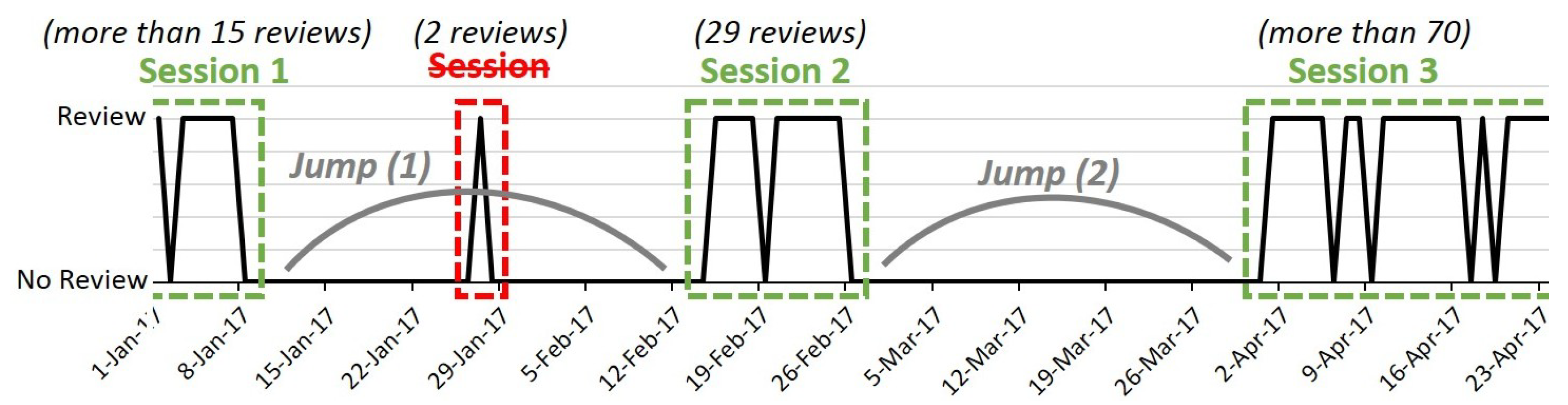
The reviews represent online resources with a linear timeline, but “gaps” in this timeline can be observed in the case of some resources such as courses. These gaps symbolize the silence of the users writing the reviews (Figure 2). This happens frequently in the case of courses because they can take place on a specific date and are not continuous. The evolution of these discontinuities is therefore correlated with the evolution of the use of the resource. In the case of courses, these interruptions last on average 35 d. In order to better estimate the contradictions and to better analyze them, the reviews were grouped according to the sessions that were formed between two discontinuities. Thus, for a given aspect, only the contradictions of the same session were examined. The sessions were defined every X days or when there was a sufficiently dense sequence of reviews. In order to obtain these groupings of reviews, the following treatment was applied:
- We computed a threshold that corresponds to the duration of the jump. This was performed on a per course basis and was based on the average time gaps between reviews (for instance, there was a gap of 35 d for the “Engagement and Nurture Marketing Strategies” lecture);
- We grouped the reviews with respect to the above-mentioned threshold, on a per course basis;
- We kept only the important sessions by suppressing the so-called “false sessions” (sessions that contained only a very low number of reviews).
Only the review clusters that had a significant number of reviews were considered for the evaluation. For instance, clusters resulting after the use of K-means [56] that contained only one or two reviews were discarded.
Algorithm 1 describes the review groupings with respect to the course sessions. The next preprocessing step was the feature extraction for the review groups.
3.1.2. Aspect Extraction
In the context of our work, the aspect represents a frequently appearing noun that has emotion expressing terms around it. For instance, the term speaker is considered as an aspect. We based our aspect extraction on the research proposed in [5]. The method is well suited to the experiments conducted over our data. In addition, we applied the following processing steps:
- The reviews corpus’ term frequency was calculated;
- The Stanford Parser https://nlp.stanford.edu:8080/parser/(accessed on 5 January 2022) was used for the parts-of-speech labeling of reviews;
- Nominal category (NN, NNS) https://cs.nyu.edu/grishman/jet/guide/PennPOS.html (accessed on 5 January 2022) terms were chosen;
- Nouns having emotive terms in a five-term context window were considered (using the SentiWordNet https://sentiwordnet.isti.cnr.it/ (accessed on 5 January 2022) dictionary);
- The extraction of the most common terms from the corpus was performed (the candidates for this step issued from the previous step). The aspects are represented by the before-mentioned terms.
Example 1.
Let D be a resource (document, e.g., course) and its associated review. Table 2 illustrates the five steps for aspect extraction from a review.
For example, “Michael is a wonderful lecturer delivering the lessons in an easy to understand manner. The whole presentation was easy to follow. I don’t recall any ambiguity in his teachings and his slide was clear. I also enjoy some of the assignments because I surprise myself by producing some great images. My main problem is the instructions of the assignments that causes a lot of students to be confused (there are many complaints expressed in the Discussion forum).”
| Algorithm 1: The reviews of a resource are grouped according to the time period (session) in which they were written. |
 |
Table 2 depicts the five steps. First, we computed the frequencies of the terms in the review set (as an example, the terms “course”, “material”, “assignment”, “content”, and “lecturer” occurred 44,219, 3286, 3118, 2947, and 2705 times, respectively). Secondly, we grammatically labeled each word (“NN” meaning singular noun and “NNS” meaning plural noun). Thirdly, only nominal category terms were selected. Fourthly, we retained only the nouns surrounded by terms belonging to the SentiWordNet dictionary (“Michael is a wonderful lecturer delivering the lessons in an easy to understand manner.”). Finally, we considered as useful aspects only those nouns that were among the most frequent in the corpus of reviews (the useful aspects in these reviews were lecturer, lesson, presentation, slide, and assignment).
After constructing the aspect list characterizing the dataset, the sentiment polarity must be computed. The sentiment analysis method used for this is described in the following section.
3.1.3. Sentiment Analysis
SentiNeuronhttps://github.com/openai/generating-reviews-discovering-sentiment (accessed on 5 January 2022), an unsupervised approach proposed in [55], was employed to detect sentiment polarity in the review-aspect. This model is based on the multiplicative Long Short-Term Memory (mLSTM), an artificial Recurrent Neural Network (RNN) architecture used in the field of deep learning. Radford et al. [55] discovered the mLSTM unit matching the output sentiment. The authors conducted a series of experiments on several test datasets, such as the review collections from Amazon [57] and IMDb https://www.cs.cornell.edu/people/pabo/movie-review-data/(accessed on 5 January 2022). This approach provides an accuracy of 91.8% and significantly outperforms several state-of-the-art approaches such as those presented in [58]. SentiNeuron yields competitive performance, compared to several state-of-the-art models. In particular, this occurs when working on movie reviews (from IMDb) and also in our situation (coursera.org reviews). We note that the term polarity means sentiment, and it is a value between −1 and 1.
3.2. Contradiction Detection and Contradiction Intensity
In this section, we introduce a model without learning, allowing the detection of contradictions and the calculation of their intensities. We considered that subjective contradictions (e.g., based on subjective elements) are related to aspects, and these are surrounded by subjective terms. We then used pieces of text called review-aspects to study the contradiction between several of these review-aspects. This model was then used as a baseline. In this paper, we propose and then compared learning methods created to detect and to estimate the intensity of the contradiction.
Definition 1.
There is a contradiction between two portions of review-aspects and containing an aspect, where , (document), when the opinions (polarities) around the aspect are opposite (i.e., ). We found that after several empirical experiments, the review-aspect was defined by a five-word snippet before and after the aspect in review .
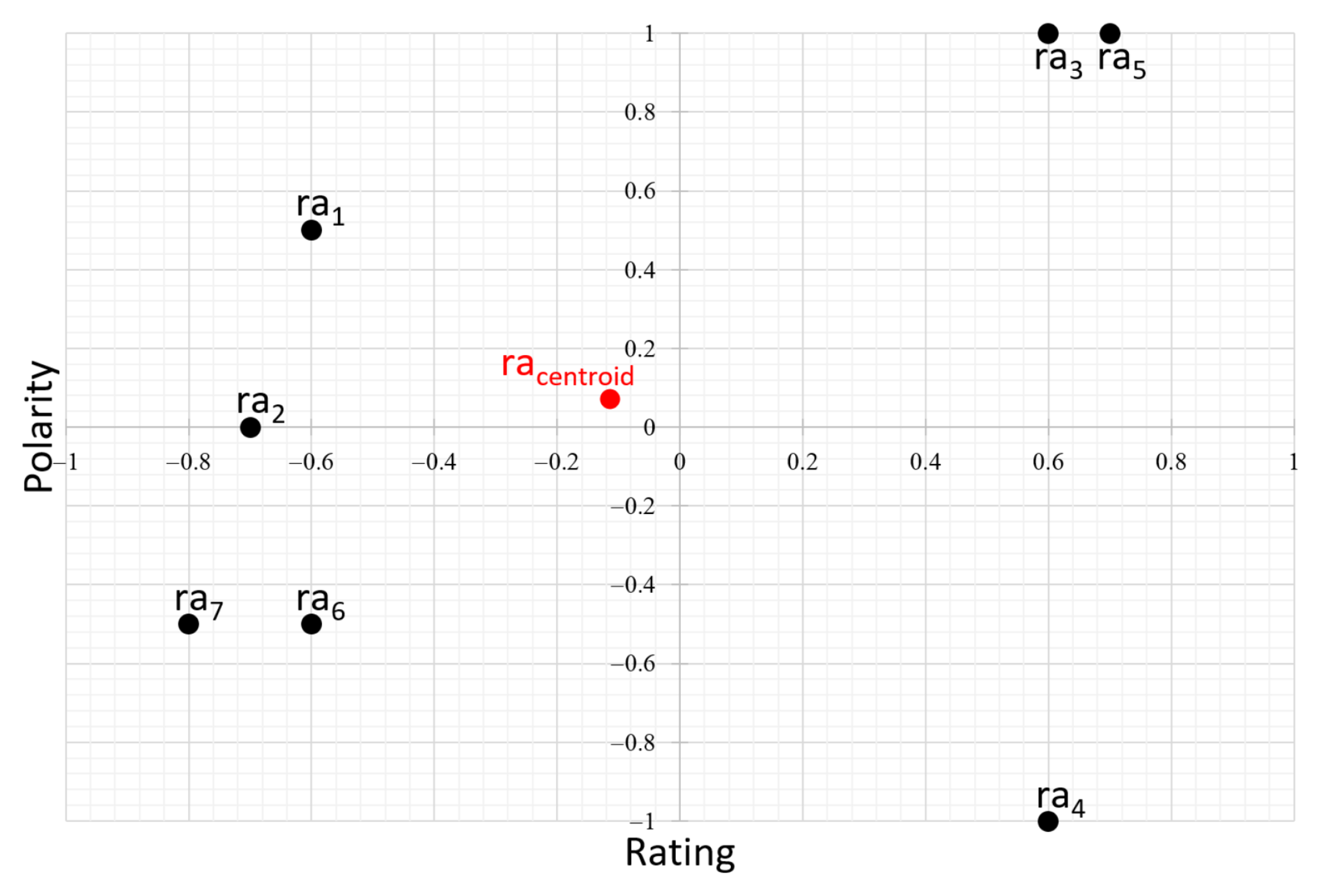
Contradiction intensity was estimated using two dimensions: polarity and rating of the review-aspect . Let each be a point on the plane with coordinates . Our hypothesis was that the greater the distance (i.e., dispersion) between the values related to each review-aspect of the same document D, the greater is the contradiction intensity. The dispersion indicator with respect to the centroid with coordinates is as follows:
represents the distance between the point of the scatter plot and the centroid (see Figure 3), and n is the number of . The two quantities and are represented on different scales; thus, their normalization becomes necessary. Since the polarity is normalized by design, we only needed to normalize the rating values. We propose the following equation for normalization: (). In what follows, the divergence from the centroid of is denoted by . Its value varies according to the following:
- is positive or zero; if , there is no dispersion = ;
- increases as moves away from . (when there is increasing dispersion).
The coordinates of the centroid were computed in two possible ways, which are described below. A simple way is to compute the average of the points; in this case, the centroid corresponds to the average point of the coordinates . Another, more refined, way is to weigh this average by the difference in absolute value between the two coordinate values (polarity and notation).
(a) The average-based centroid. In this scenario, the centroid’s coordinates were calculated as follows using the average of polarities and ratings:
(b) The weighted average-based centroid. In this scenario, the centroid coordinates were the weighted average of ratings and polarities:
where n is the number of points . The coefficient was computed as follows:
For a data point, if the values of the two dimensions were farther apart, our assumption was that such a point should be considered of high importance. We hypothesized that a positive aspect in a low-rating review should have a higher weight, and vice versa. Therefore, an importance coefficient was computed for each data point, based on the absolute value difference between the values over both dimensions. The division by represents a normalization by the maximum value of the difference in absolute value () and n. For instance, for a polarity of and a rating of 1, the coefficient is (), and for a polarity of 1 and a rating of 1, the coefficient is 0 ().
3.3. Predicting Contradiction Intensity
Our model without learning has the advantage of being easy to implement and of not requiring a corpus. However, we had to tackle the issues of the selection of the most relevant and fruitful features for the measurement of the contradiction intensity. Indeed, as long as we did not try all the configurations of the features (rating, polarity), it was not possible to properly judge the efficiency of each of these features, nor to identify the best ones for this task. In addition, the previously presented computation method (Section 3.2) was simply based on a dispersion formula of the two scores associated with polarity and rating. In the present more in-depth study, we employed feature selection methods to determine the best-performing features (derived from the rating, polarity, and review) to consider in the contradiction intensity measurement task. The attribute selection methods aim to suppress the maximum amount of non-relevant and redundant information before the learning process [59]. They also automatically pick the subsets of features that produce the greatest results. This phase highlighted several sets of features. Thus, we evaluated the effectiveness of these sets by applying them to learning techniques in a specific context: the estimation of the intensity of contradiction in text (reviews left by users on MOOC resources). The learning techniques used are techniques that have proven successful in many tasks. We chose to use SVM, decision trees (J48), and naive Bayes for the first experiments. The results obtained based on feature selection were compared to those of our method without learning, in order to measure the potential gain brought in by such techniques.
4. Experimental Evaluation
This section presents the performed experiments and their results. After the introduction of our corpus and its study, the section presents and discusses the results obtained in the presence of our baseline. We then present the experiments that allowed us to select the features that gave the best results with the learning-based algorithms. The section ends with a presentation and comparison of the results obtained with the SVM, J48, and naive Bayes algorithms.
4.1. Description of the Test Dataset
This section presents in detail the corpus on which we based our experiments. It then presents how the corpus was obtained by means of a study of the annotations made for the qualification of the intensity of contradictions and for the analysis of feeling.
4.1.1. Data
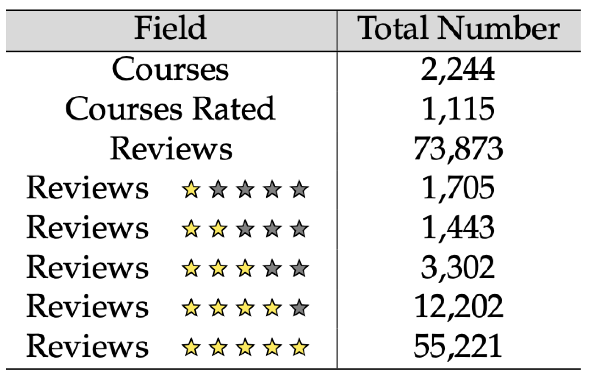
We are not aware of the existence of a standard dataset for evaluating the contradiction intensity (strength). Therefore, we built our own dataset by collecting 73,873 reviews and their ratings corresponding to 2244 English courses from coursera.org via its API https://building.coursera.org/app-platform/catalog (accessed on 5 January 2022) and web page parsing. This was performed during the time interval 10–14 October 2016. More detailed statistics on this Coursera dataset are depicted in Figure 4. Our entire test dataset, as well as its detailed statistics are publicly available https://pageperso.lis-lab.fr/ismail.badache/Reviews_ExtracTerms%20HTML/ (accessed on 5 January 2022).
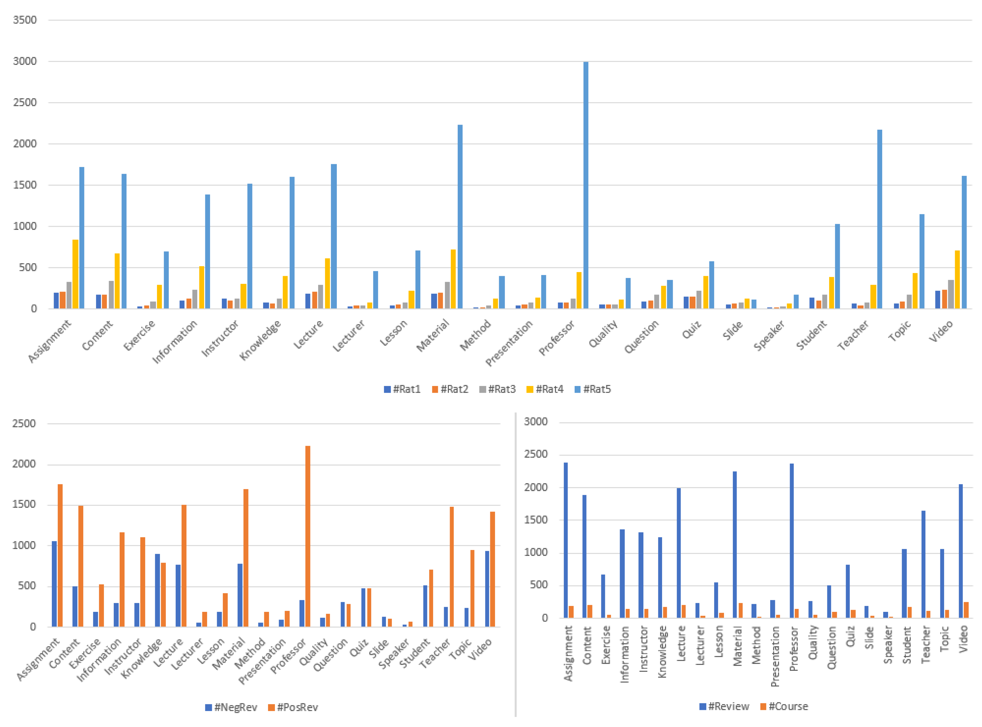
We were able to automatically capture 22 useful aspects from the set of reviews (see Figure 5). Figure 5 presents the statistics on the 22 detected aspects, for example for the Slide aspect, we recorded: 56 one-star ratings, 64 two-star ratings, 81 three-star ratings, 121 four-star ratings, 115 five-star ratings, 131 reviews with negative polarity, 102 reviews with positive polarity, as well as 192 reviews and 41 courses concerning this aspect.
4.1.2. User Study
For a given aspect, in order to obtain contradiction and sentiment judgments, we conducted a user study as follows:
- The sentiment class for each review-aspect of 1100 courses was assessed by 3 users (assessors). Users must only judge the polarity of the involved sentiment class;
- The degree of contradiction between these review-aspects (see Figure 6) was assessed by 3 new users.
Annotation corresponding to the above judgment was performed manually. For each aspect, on average, 22 review-aspects per course were judged (in total: 66,104 review-aspects of 1100 courses, i.e., 50 courses for each aspect). Exactly 3 users evaluated each aspect.
A 3-level assessment scale (Negative, Neutral, Positive) was employed for the sentiment evaluation in the review-aspects, in a per-course manner, and a 5-level assessment scale (Very Low, Low, Strong, Very Strong, and Not Contradictory) was employed for the contradiction evaluation, as depicted in Figure 6.
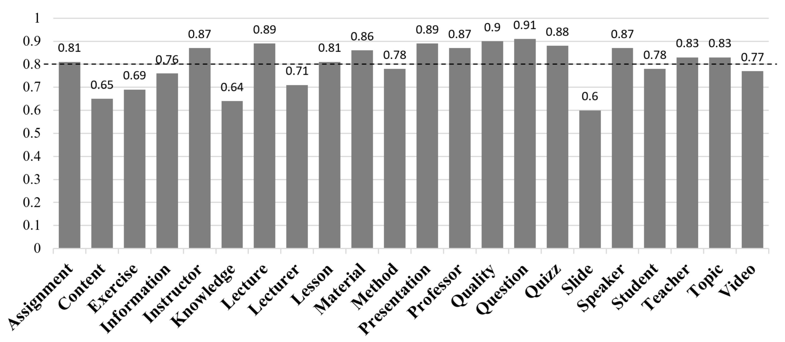
Using Cohen’s Kappa coefficient k [60], we estimated the agreement degree among the assessors for each aspect. In order to obtain a unique Kappa value, we calculated the pairwise Kappa of assessors, and then, we computed the average.
For each aspect from all the reviews, the distribution of the Kappa values is shown in Figure 7. The variation of the measure of agreement was between and . Among the assessors, the average level of agreement was equal to 80%. Such a score corresponds to a strong agreement. Between the assessors who performed the sentiment annotation, the Kappa coefficient value was (78% agreement), which also indicates a substantial agreement.
4.2. Results and Discussion
This section presents the results obtained first using the learning-free model. We compared the results obtained with and without the use of review sessions and considering both the average-based centroid and the weighted average-based centroid scenarios (see Section 3.2) in turn. We studied the influence of the sentiment analysis algorithm on the results. We then compared the results obtained through the selection of features and the use of learning-based models such as SVM, decision trees, and naive Bayes.
4.2.1. Averaged and Weighted Centroid
In order to quantify the effectiveness of our proposal, we employed the same performance measure as for the SemEval competition https://alt.qcri.org/semeval2016/task7/ (accessed on 5 January 2022), that is to say, the correlation coefficient. We used Pearson’s correlation coefficient, which considers our results against the annotator’s judgments. The second performance measure was the precision (the number of correct estimations divided by the total number of estimations).
We must mention that:
- The training phase for the sentiment analysis was performed over 50 k reviews issued from the IMDb movie database https://ai.stanford.edu/~amaas/data/sentiment/ (the vocabulary used in the movie reviews is similar to the vocabulary used in our dataset);
- The accuracy of the sentiment analysis rose to ;
- The assessed sentiment judgments were considered as the ground truth, thus yielding 100% in terms of accuracy.
The results of our two centroid strategies—Config (1), averaged centroid—and Config (2), weighted centroid—are depicted in Table 3 and in Table 4, respectively. Both configurations have the variants WITHOUT review sessions (Table 3) and WITH review sessions (Table 4). In order to validate the statistical significance of the improvements (for both WITH and WITHOUT), compared with their respective baselines, we applied the paired Student’s t-test. The statistical significance of the improvements, when p-value < 0.05 and p-value < 0.01, is represented in the tables by and , respectively. Next, we discuss the results.
(a) WITHOUT review sessions.
Config (1): averaged centroid. The averaged centroid dispersion measure yielded positive correlation values (moderate or even high) with respect to our annotator’s judgments (Pearson: , , ). The hypothesis was that having widely opposite review-aspect polarities would imply review-aspects divergent from the centroid, thus a highly intense dispersion. Moreover, when considering the users’ sentiment judgments (Table 3 (b)), we obtained better results than when considering sentiment analysis models (Table 3, baseline and (a)). The improvements went from for (baseline) (Pearson: 0.45, compared to 0.61) to for (b) (Pearson: 0.45, compared to 0.68). The correlation coefficient conclusions stand for the precision as well. One may notice that a loss of in terms of sentiment analysis accuracy (100–79%) led to a loss in terms of precision.
Config (2): weighted centroid. This configuration yielded positive correlation values as well (, , ). One may note that the results when considering the weight of the centroids were better than when this particular weight was ignored. Compared to the averaged centroid (Config (1)), the improvements were 13% for naive Bayes, 31% for SentiNeuron, and 28% for the manual judgments, respectively. This trend was confirmed for the precision results as well. Thus, the sentiment analysis model significantly impacted the estimation quality of the studied contradictions.
(b) WITH review sessions
The correlation values remained positive when considering the review sessions, for both configurations (averaged and weighted centroids), as reflected in Table 4. This occurred for the two assumptions concerning sentiment analysis accuracy (i.e., 79% and 100%). This suggests that the impact of the sentiment analysis model was quite significant. In fact, the drop of of sentiment accuracy implies an average drop of in terms of contradiction detection performance. The performance was improved when considering the review sessions, compared to the results without the review sessions.
Config (1): averaged centroid. The results obtained with SentiNeuron (a) and with user judgments (b) (Table 4) were constantly better than in the case of the same scenarios without review sessions (Table 3). Thus, grouping the reviews by session was helpful for the contradiction intensity quantification ( and in terms of precision, for Scenarios (a) and (b), respectively). In addition, the contradiction intensity may be fairly estimated when considering only the reviews issued from one particular session.
Config (2): weighted centroid. This configuration was the best possible one. It had the strongest baseline, both in terms of Pearson’s correlation coefficient and precision, and also the highest possible value, both in terms of precision () and correlation coefficient (), amongst all configurations. Its strengths were represented by the weights assigned to the centroids and also by the grouping of the reviews according to their session (the time dimension).
To sum up, we noticed that the proposed approach performed well for every configuration that we considered. Config (2), coupled with the review sessions, yielded the best performance. The t-tests proved that the improvements were statistically significant with respect to the baselines. We hypothesized that the three-step preprocessing helped with the performance improvements, the clustering of reviews with respect to their course sessions being helpful in particular. When the sentiment analysis method performed well, the global results were also improved.
4.2.2. Best Feature Identification
In order to identify the most powerful features that estimated the contradiction intensity within our experiments, we considered several feature selection algorithms [59]. The aim of this type of algorithm is to filter out as much as possible the information redundancy in the dataset. In terms of framework, we employed the open-source tool called Weka https://www.cs.waikato.ac.nz/ml (accessed on 5 January 2022). This tool is written in Java, and it provides a wide spectrum of machine learning models and feature selection algorithms.
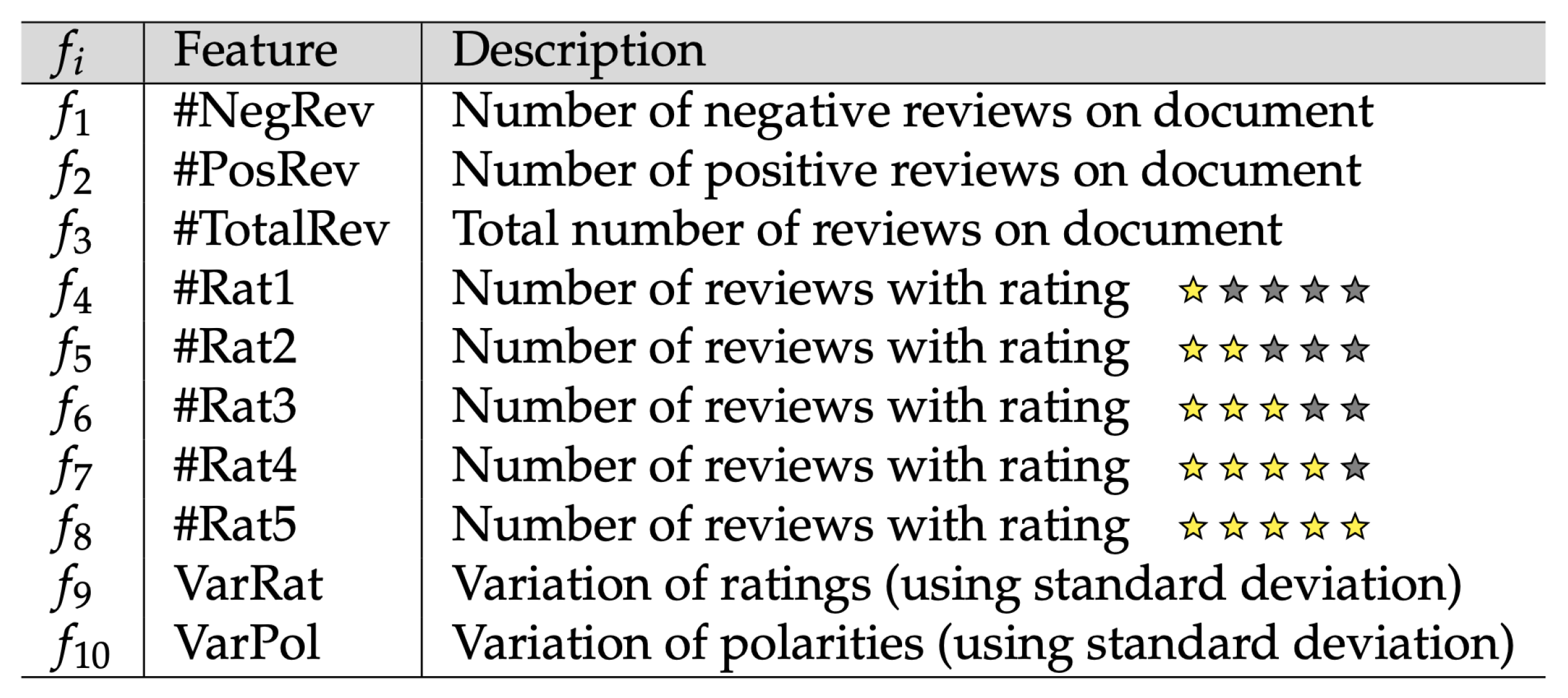
Figure 8 illustrates the 10 features we considered for the contradiction intensity prediction within the comments. The nature of the features to is given by a simple count, e.g., the polarity criteria and represent the number of negative and positive comments in the document, respectively. Criteria , , , , and are related to scoring. The rating may have values from one to five, where three means “average” and five means “excellent”. Concerning the last two attributes, and , they represent the variation in the ratings and polarities of the comments for a given aspect associated with a document (a course in our case). These two criteria were calculated based on the following standard deviation formula, proposed in [61]:
where x represents the feature value (ex.: scoring, polarity), is the sample mean of the criterion concerned, and n is the sample size.
For the experiments, 50 courses were randomly selected from the dataset, for each of the 22 aspects. Thus, we obtained a total of 1100 courses (instances). The intensity contradiction classes were then established, with respect to specific aspects. There were four classes: Very Low (230 courses), Low (264 courses), Strong (330 courses), and Very Strong (276 courses), with respect to the judgments provided by the annotators.
Since the distribution of the courses by class was not balanced and in order to avoid a possible model bias that would assign more observations than normal to the majority class, we applied a sub-sampling approach, and we obtained a balanced collection of 230 individuals by class, therefore a total of 920 courses.
After obtaining the balanced dataset, we applied the feature selection mechanisms on it. We performed five-fold cross-validation (a machine learning step widely employed for hyperparameter optimization).
The feature selection algorithms output feature significance scores for the four established classes. Their inner workings are different. They may be based on feature importance ranking (e.g., FilteredAttributeEval), or on the feature selection frequency during the cross-validation step (e.g., FilteredSubsetEval). We mention that we employed the default Weka parameter settings for these methods.
Since we applied five-fold cross-validation over the ten features, . The results concerning the selected features are summarized in Figure 9. There were two classes of selection algorithms:
- Based on ranking metrics to sort the features (marked by Rank in the figure);
- Based on the occurrence frequency during the cross-validation step (marked by #Folds in the figure).
One may note that a good feature has either a high rank or a high frequency.
The strongest features, by both the #Folds and the Rank metrics, were : VarPol, : VarRat, : #NegRev, and : #PosRev. The features with average importance were : #TotalRev, : #Rat1, and : #Rat5, except for the case of CfsSubsetEval, for which the features and were not selected. The weakest features were : #Rat2, : #Rat3, and : #Rat4.
4.2.3. Feature Learning Process for Contradiction Intensity Prediction
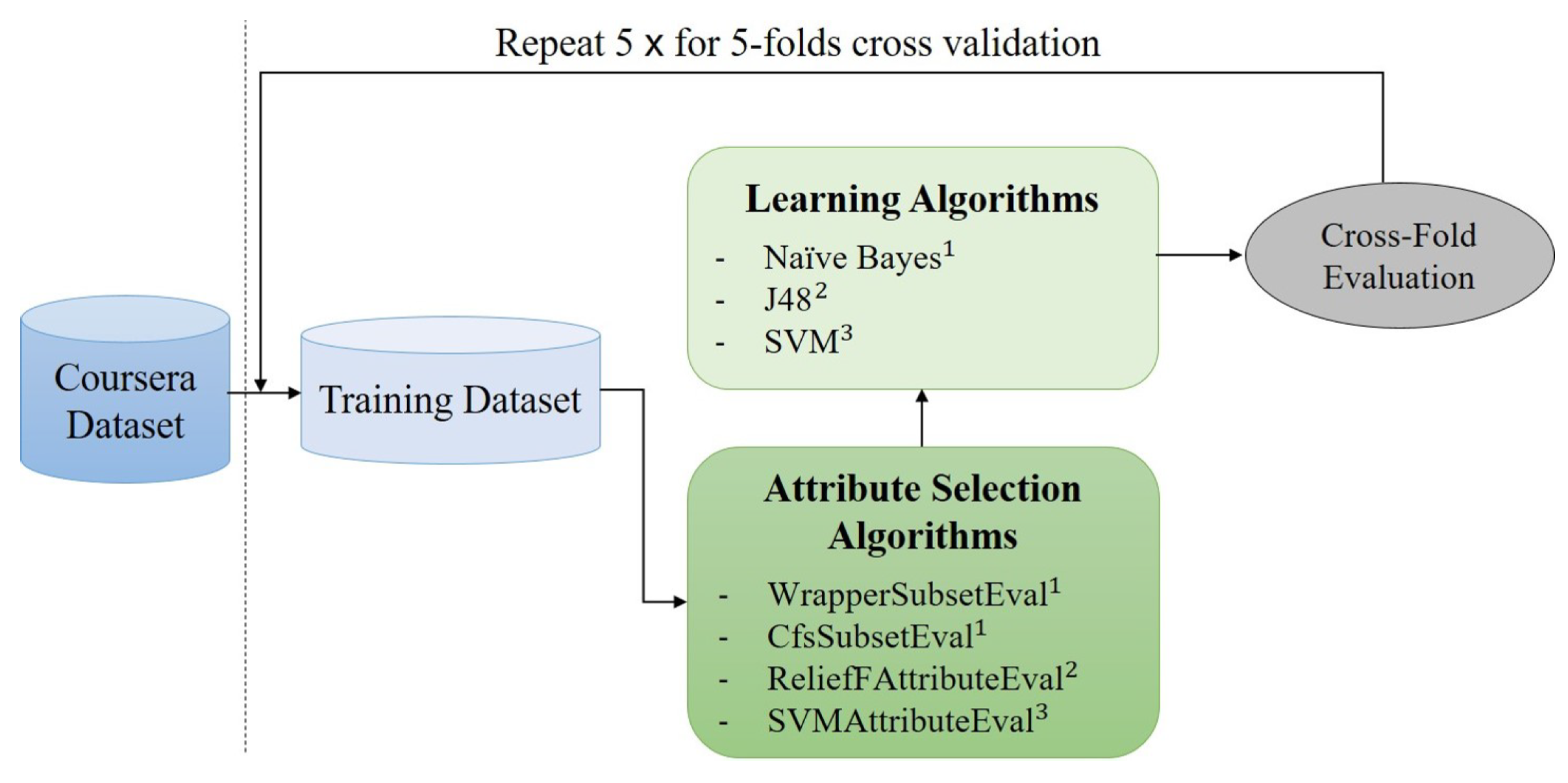
More tests were conducted, based on the proposed and discussed features. The instances (courses) corresponding to the 22 aspects were employed as the training data. Based on the confirmed effectiveness of the SVM [62], J48 (C4.5 implementation) [63], and naive Bayes [64] algorithms in the context of textual data analysis, we employed them in our study as well. The input is represented by a feature vector (please refer to Figure 8), with two possible scenarios: all the features together or the selected features as seen in the previous section. Then, the learning process estimates the corresponding contradiction class, that is to say Very Low, Low, Strong, or Very Strong. Five-fold cross-validation was applied for these experiments as well.
Figure 10 illustrates the learning process we put in place for the evaluation of the criteria.
Let us recall that the feature selection step yielded the following feature sets (see Table 5):
- For the CfsSubsetEval and the WrapperSubsetEval algorithms, the selected features were: : #NegRev, : #PosRev, : #TotalRev, : VarRat, and : VarPol;
- For CfsSubsetEval, the selected features were: , , , , and ;
- For the CfsSubsetEval and the WrapperSubsetEval algorithms, the selected features were: , , , , and ;
- For the other algorithms, all the features were selected: : #NegRev, : #PosRev, : #TotalRev, : #Rat1, : #Rat2, : #Rat3, : #Rat4, : #Rat5, : VarRat, and : VarPol.
Regarding the input feature vector, we needed to decide how many features to consider, either all of them or only those proposed by feature selection. For the latter, we must decide what should be the machine learning algorithm to exploit them.
This type of discussion was conducted by Hall and Holmes [59]. They argued about the effectiveness of several feature selection methods by crossing them with several machine learning algorithms. They matched the best feature selection and machine learning techniques, since they noticed varying performance during the experiments. Inspired by their findings [59], we used the following couples of learning methods and feature selection algorithms:
- Feature selection: CfsSubsetEval (CFS) and WrapperSubsetEval (WRP); machine learning algorithm: naive Bayes;
- Feature selection: ReliefFAttributeEval (RLF); machine learning algorithm: J48 (the C4.5 implementation);
- Feature selection: SVMAttributeEval (SVM); machine learning algorithm: multi-class SVM (SMO function on Weka).
The naive Bayes algorithm represents the baseline, and statistical significance tests (paired t-test) were conducted to compare the performances. The results are shown in Table 6. Significance (p-value < 0.05) is marked by , and strong significance (p-value < 0.01) is marked by , in the table. We next discuss the obtained results.
The results with the naive Bayes model: This model yielded precision values of 0.72 and 0.68, corresponding to the WRP and the CFS feature selection algorithms, respectively. The feature selection algorithms overcame the performance obtained when considering all the features, which maxed out at 0.60, in terms of precision. Thus, the feature selection mechanisms helped the learning process of the machine learning algorithms. The classes for which the highest precision was obtained were Very Low, Strong, and Very Strong. The remaining class, Low, could not yield more than 0.46 in terms of precision, in the case of the WRP selection algorithm.
The results with the SVM model: This model yielded better performance, compared to the naive Bayes classifier. The relative improvements of the SVM model, compared to naive Bayes, went from in the case of WRP to in the case of CFS. One should note that this model managed to yield better performance for the difficult class (Low). The feature selection algorithm SVMAttributeEval did not improve the performance, compared to considering all the features together. This behavior may occur because the performance was already quite high.
The results with the J48 model: This decision trees model yielded the best performance in terms of precision, when considering all the features. The relative improvements were 17%, with respect to the SVM model, 33% with respect to the naive Bayes model with the WRP selection algorithm, and finally, 41% with respect to the naive Bayes model with the CFS selection. The most difficult class for the other models, Low, obtained a performance of 92% in terms of precision, meaning relative improvements ranging from 28% to 142%, with respect to the other learning models. Moreover, the improvements were significant for all the involved classes. On the other hand, feature selection did not bring any improvement this time. As for the SVM model, this non-improvement must surely be due to the fact that the performance of the algorithm was already extremely high, and consequently, the impact of feature selection was very marginal.
In what follows, we compared the best results obtained by the two methods of contradiction intensity estimation. We refer to the unsupervised method, based on the review-aspect dispersion function taking into account the review sessions (as in Table 4), and to the supervised method, based on several features extracted by the selection algorithms within the learning process (see the average precision in Table 6). In terms of precision, naive Bayes used with the CFS feature selection algorithm registered the lowest precision result (68%), as can be seen in Table 4 and Table 6. SVM performed relatively better than the unsupervised method with all of its configurations using an averaged centroid. Moreover, SVM even outperformed naive Bayes used with CFS and WRP with an improvement rate of 21% and 14%, respectively. However, the majority of the results obtained with the unsupervised method using the weighted centroid significantly outperformed those obtained using the averaged centroid or even those obtained by the supervised method using naive Bayes and SVM. In all these experiments, the best results were obtained by the J48 decision trees algorithm using the RLF selection algorithm. J48 recorded significant improvement rates over all other configurations, using both supervised and unsupervised methods: 17%, 33%, and 41%, over SVM, naive Bayes (WRP), and naive Bayes (CFS), respectively. Table 7 shows in detail the different improvement rates between J48 and the other configurations.
To sum up, the results clearly showed that the contradiction intensity can be predicted by the J48 machine learning model, with good performance. The feature selection methods proved to be effective for one case out of three, with respect to the learning models (for naive Bayes). This similar performance between the versions with and without feature selection shows that, after a certain performance level yielded by the machine learning algorithm, the feature selection impact stayed quite limited. We conclude that the courses having highly divergent reviews were prone to containing contradictions with several intensity levels.
5. Conclusions
This research focused on the estimation of the contradiction intensity in texts, more in particular in MOOC course reviews. Unlike most other authors, we did not only try to find out if a contradiction occurred, but we were concerned with measuring its strength. The contradiction was identified around the aspects that generated the difference in opinions within the reviews. We hypothesized that the contradiction occurred when the sentiment polarities around these aspects were divergent. This paper’s proposal to quantify the contradiction intensity was twofold, consisting of an unsupervised approach and a supervised one, respectively. Within the unsupervised approach, the review-aspects were represented as a function that estimated the dispersion (more intense contradictions occurred when the sentiment polarities and the ratings were dispersed in the bi-dimensional space characterized by sentiment polarity and ratings, respectively). The other idea was to group the reviews by sessions (the time dimension), allowing an effective treatment to avoid fake contradictions. The supervised approach considered several features and learned to predict the contradiction intensity. We hypothesized that the ratings and the sentiment polarities around an aspect may be useful as features to estimate the intensity of the contradictions. When the sentiment polarities and the ratings were diverse (in terms of the standard deviation), the chances of the contradictions being intense increased.
For the unsupervised approach, the weighted centroid configuration, coupled with the review sessions (considering the time dimension of the reviews), yielded the best performances.
For the supervised approach, the features VarPol, VarRat, #PosRev, VarRat, and #NegRev had the best chances to correctly predict the intensity classes for the contradictions. The feature selection study prove to be effective for one case out of three, with respect to the learning models (for naive Bayes). Thus, feature selection may be beneficial for the learning models that did not perform very well. The best performance was obtained by the J48 decision trees algorithm. This model was followed, in terms of precision, by the SVM model and, lastly, by the naive Bayes model.
The most important limitation of our proposal is that the models depend on the quality of the sentiment polarity estimation and of the aspect extraction method. That is why our future work will focus on finding ways of selecting methods for sentiment polarity estimation and aspect extraction that would be the most appropriate for this task.
Additionally, we aim to conduct larger-scale experiments, over various data types, since the so far, the promising results motivated us to investigate this topic even further.
Author Contributions
Conceptualization, A.-G.C. and S.F.; Data curation, I.B.; Formal analysis, I.B.; Supervision, S.F.; Validation, A.-G.C.; Writing (original draft), I.B., A.-G.C. and S.F.; Writing (review and editing), I.B., A.-G.C. and S.F. All authors have read and agreed to the published version of the manuscript.
Funding
This research received no external funding.
Institutional Review Board Statement
Not applicable.
Informed Consent Statement
Not applicable.
Data Availability Statement
Not applicable.
Conflicts of Interest
The authors declare no conflict of interest.
References
- Badache, I.; Boughanem, M. Harnessing Social Signals to Enhance a Search. IEEE/WIC/ACM 2014, 1, 303–309. [Google Scholar]
- Badache, I.; Boughanem, M. Emotional social signals for search ranking. SIGIR 2017, 3, 1053–1056. [Google Scholar]
- Badache, I.; Boughanem, M. Fresh and Diverse Social Signals: Any impacts on search? In Proceedings of the CHIIR ’17: Proceedings of the 2017 Conference on Conference Human Information Interaction and Retrieval, Oslo, Norway, 7–11 March 2017; pp. 155–164. [Google Scholar]
- Kim, S.; Zhang, J.; Chen, Z.; Oh, A.H.; Liu, S. A Hierarchical Aspect-Sentiment Model for Online Reviews. In Proceedings of the Twenty-Seventh AAAI Conference on Artificial Intelligence, Bellevue, WA, USA, 14–18 July 2013. [Google Scholar]
- Poria, S.; Cambria, E.; Ku, L.; Gui, C.; Gelbukh, A.F. A Rule-Based Approach to Aspect Extraction from Product Reviews. In Proceedings of the Second Workshop on Natural Language Processing for Social Media, SocialNLP@COLING 2014, Dublin, Ireland, 24 August 2014; pp. 28–37. [Google Scholar] [CrossRef] [Green Version]
- Wang, L.; Cardie, C. A Piece of My Mind: A Sentiment Analysis Approach for Online Dispute Detection. In Proceedings of the 52nd Annual Meeting of the Association for Computational Linguistics, ACL 2014, Baltimore, MD, USA, 22–27 June 2014; Short Papers. Volume 2, pp. 693–699. [Google Scholar]
- Harabagiu, S.M.; Hickl, A.; Lacatusu, V.F. Negation, Contrast and Contradiction in Text Processing. In Proceedings of the Twenty-First National Conference on Artificial Intelligence and the Eighteenth Innovative Applications of Artificial Intelligence Conference, Boston, MA, USA, 16–20 July 2006; pp. 755–762. [Google Scholar]
- de Marneffe, M.; Rafferty, A.N.; Manning, C.D. Finding Contradictions in Text. In Proceedings of the 46th Annual Meeting of the Association for Computational Linguistics, Columbus, OH, USA, 15–20 June 2008; pp. 1039–1047. [Google Scholar]
- Tsytsarau, M.; Palpanas, T.; Denecke, K. Scalable discovery of contradictions on the web. In Proceedings of the 19th International Conference on World Wide Web, WWW 2010, Raleigh, NC, USA, 26–30 April 2010; pp. 1195–1196. [Google Scholar] [CrossRef] [Green Version]
- Tsytsarau, M.; Palpanas, T.; Denecke, K. Scalable detection of sentiment-based contradictions. DiversiWeb WWW 2011, 11, 105–112. [Google Scholar]
- Yazi, F.S.; Vong, W.T.; Raman, V.; Then, P.H.H.; Lunia, M.J. Towards Automated Detection of Contradictory Research Claims in Medical Literature Using Deep Learning Approach. In Proceedings of the 2021 Fifth International Conference on Information Retrieval and Knowledge Management (CAMP), Pahang, Malaysia, 15–16 June 2021; pp. 116–121. [Google Scholar] [CrossRef]
- Hsu, C.; Li, C.; Sáez-Trumper, D.; Hsu, Y. WikiContradiction: Detecting Self-Contradiction Articles on Wikipedia. In Proceedings of the IEEE International Conference on Big Data (IEEE BigData 2021), Orlando, FL, USA, 15–18 December 2021. [Google Scholar]
- Sepúlveda-Torres, R. Automatic Contradiction Detection in Spanish. In Proceedings of the Doctoral Symposium on Natural Language Processing from the PLN.net Network, Baeza, Spain, 19–20 October 2021. [Google Scholar]
- Rahimi, Z.; Shamsfard, M. Contradiction Detection in Persian Text. arXiv 2021, arXiv:2107.01987. [Google Scholar]
- Pielka, M.; Sifa, R.; Hillebrand, L.P.; Biesner, D.; Ramamurthy, R.; Ladi, A.; Bauckhage, C. Tackling Contradiction Detection in German Using Machine Translation and End-to-End Recurrent Neural Networks. In Proceedings of the 2020 25th International Conference on Pattern Recognition (ICPR), Milan, Italy, 10–15 January 2021; pp. 6696–6701. [Google Scholar] [CrossRef]
- Păvăloaia, V.D.; Teodor, E.M.; Fotache, D.; Danileţ, M. Opinion Mining on Social Media Data: Sentiment Analysis of User Preferences. Sustainability 2019, 11, 4459. [Google Scholar] [CrossRef] [Green Version]
- Mohammad, S.M.; Turney, P.D. Crowdsourcing a word–Emotion association lexicon. Comput. Intell. 2013, 29, 436–465. [Google Scholar] [CrossRef] [Green Version]
- Al-Ayyoub, M.; Rabab’ah, A.; Jararweh, Y.; Al-Kabi, M.N.; Gupta, B.B. Studying the controversy in online crowds’ interactions. Appl. Soft Comput. 2018, 66, 557–563. [Google Scholar] [CrossRef]
- Popescu, A.M.; Pennacchiotti, M. Detecting controversial events from twitter. In Proceedings of the 19th ACM International Conference on Information and Knowledge Management, Toronto, ON, Canada, 26–30 October 2010; pp. 1873–1876. [Google Scholar]
- Balasubramanyan, R.; Cohen, W.W.; Pierce, D.; Redlawsk, D.P. Modeling polarizing topics: When do different political communities respond differently to the same news? In Proceedings of the Sixth International AAAI Conference on Weblogs and Social Media, Dublin, Ireland, 4–8 June 2012.
- Dori-Hacohen, S.; Allan, J. Detecting controversy on the web. In Proceedings of the 22nd ACM international conference on Information & Knowledge Management, San Francisco, CA, USA, 27 October–1 November 2013; pp. 1845–1848. [Google Scholar]
- Dori-Hacohen, S.; Allan, J. Automated Controversy Detection on the Web. In Advances in Information Retrieval; Hanbury, A., Kazai, G., Rauber, A., Fuhr, N., Eds.; Springer International Publishing: Cham, Germany, 2015; pp. 423–434. [Google Scholar]
- Garimella, K.; Morales, G.D.F.; Gionis, A.; Mathioudakis, M. Quantifying Controversy in Social Media. In Proceedings of the Ninth ACM International Conference on Web Search and Data Mining, San Francisco, CA, USA, 22–25 February 2016; pp. 33–42. [Google Scholar] [CrossRef] [Green Version]
- Guerra, P.C.; Meira, W., Jr.; Cardie, C.; Kleinberg, R. A measure of polarization on social media networks based on community boundaries. In Proceedings of the Seventh International AAAI Conference on Weblogs and Social Media, Cambridge, MA, USA, 8–11 July 2013. [Google Scholar]
- Jang, M.; Allan, J. Improving Automated Controversy Detection on the Web. In Proceedings of the 39th International ACM SIGIR Conference on Research and Development in Information Retrieval, SIGIR 2016, Pisa, Italy, 17–21 July 2016; pp. 865–868. [Google Scholar] [CrossRef] [Green Version]
- Lin, W.H.; Hauptmann, A. Are these documents written from different perspectives? A test of different perspectives based on statistical distribution divergence. In Proceedings of the 21st International Conference on Computational Linguistics and the 44th Annual Meeting of the Association for Computational Linguistics, Association for Computational Linguistics, Sydney, Australia, 6–8 July 2006; pp. 1057–1064. [Google Scholar]
- Sriteja, A.; Pandey, P.; Pudi, V. Controversy Detection Using Reactions on Social Media. In Proceedings of the 2017 IEEE International Conference on Data Mining Workshops (ICDMW), New Orleans, LA, USA, 18–21 November 2017; pp. 884–889. [Google Scholar]
- Morales, A.; Borondo, J.; Losada, J.C.; Benito, R.M. Measuring political polarization: Twitter shows the two sides of Venezuela. Chaos Interdiscip. J. Nonlinear Sci. 2015, 25, 033114. [Google Scholar] [CrossRef] [PubMed] [Green Version]
- Garimella, K.; Morales, G.D.F.; Gionis, A.; Mathioudakis, M. Quantifying Controversy on Social Media. Trans. Soc. Comput. 2018, 1. [Google Scholar] [CrossRef] [Green Version]
- Ahmed, A.; Xing, E.P. Staying informed: Supervised and semi-supervised multi-view topical analysis of ideological perspective. In Proceedings of the 2010 Conference on Empirical Methods in Natural Language Processing, Association for Computational Linguistics, Stroudsburg, PA, USA, 9–11 October 2010; pp. 1140–1150. [Google Scholar]
- Cohen, R.; Ruths, D. Classifying political orientation on Twitter: It’s not easy! In Proceedings of the Seventh International AAAI Conference on Weblogs and Social Media, Cambridge, MA, USA, 8–11 July 2013.
- Conover, M.D.; Gonçalves, B.; Ratkiewicz, J.; Flammini, A.; Menczer, F. Predicting the political alignment of twitter users. In Proceedings of the 2011 IEEE Third International Conference on Privacy, Security, Risk and Trust and 2011 IEEE Third International Conference on Social Computing, Boston, MA, USA, 9–11 October 2011; pp. 192–199. [Google Scholar]
- Paul, M.; Girju, R. A Two-Dimensional Topic-Aspect Model for Discovering Multi-Faceted Topics. In Proceedings of the AAAI’10: Twenty-Fourth AAAI Conference on Artificial Intelligence, Atlanta, GA, USA, 11–15 July 2010; AAAI Press: Atlanta, GA, USA, 2010; pp. 545–550. [Google Scholar]
- Qiu, M.; Jiang, J. A Latent Variable Model for Viewpoint Discovery from Threaded Forum Posts. In Proceedings of the 2013 Conference of the North American Chapter of the Association for Computational Linguistics: Human Language Technologies, Atlanta, Georgia, 9–14 June 2013; Association for Computational Linguistics: Atlanta, GA, USA, 2013; pp. 1031–1040. [Google Scholar]
- Trabelsi, A.; Zaiane, O.R. Mining contentious documents using an unsupervised topic model based approach. In Proceedings of the 2014 IEEE International Conference on Data Mining, Shenzhen, China, 14–17 December 2014; pp. 550–559. [Google Scholar]
- Thonet, T.; Cabanac, G.; Boughanem, M.; Pinel-Sauvagnat, K. VODUM: A topic model unifying viewpoint, topic and opinion discovery. In European Conference on Information Retrieval; Spring: Berlin/Heidelberg, Germany, 2016; pp. 533–545. [Google Scholar]
- Galley, M.; McKeown, K.; Hirschberg, J.; Shriberg, E. Identifying agreement and disagreement in conversational speech: Use of bayesian networks to model pragmatic dependencies. In Proceedings of the 42nd Annual Meeting on Association for Computational Linguistics, Stroudsburg, PA, USA, 21–26 July 2004; p. 669. [Google Scholar]
- Menini, S.; Tonelli, S. Agreement and disagreement: Comparison of points of view in the political domain. In Proceedings of the COLING 2016, the 26th International Conference on Computational Linguistics, Technical Papers, Osaka, Japan, 11–16 December 2016; pp. 2461–2470. [Google Scholar]
- Mukherjee, A.; Liu, B. Mining contentions from discussions and debates. In Proceedings of the 18th ACM SIGKDD International Conference on Knowledge Discovery and Data Mining, Beijing, China, 12–16 August 2012; pp. 841–849. [Google Scholar]
- Mohammad, S.; Kiritchenko, S.; Zhu, X. NRC-Canada: Building the State-of-the-Art in Sentiment Analysis of Tweets. In Proceedings of the 7th International Workshop on Semantic Evaluation, SemEval@NAACL-HLT 2013, Atlanta, GA, USA, 14–15 June 2013; pp. 321–327. [Google Scholar]
- Mohammad, S.; Kiritchenko, S.; Sobhani, P.; Zhu, X.; Cherry, C. SemEval-2016 Task 6: Detecting Stance in Tweets. In Proceedings of the 10th International Workshop on Semantic Evaluation (SemEval-2016), San Diego, CA, USA, 10–11 June 2016; Association for Computational Linguistics: San Diego, CA, USA; pp. 31–41. [Google Scholar] [CrossRef]
- Augenstein, I.; Rocktäschel, T.; Vlachos, A.; Bontcheva, K. Stance detection with bidirectional conditional encoding. arXiv 2016, arXiv:1606.05464. [Google Scholar]
- Gottipati, S.; Qiu, M.; Sim, Y.; Jiang, J.; Smith, N. Learning topics and positions from debatepedia. In Proceedings of the 2013 Conference on Empirical Methods in Natural Language Processing, Seattle, WA, USA, 18–21 October 2013; pp. 1858–1868. [Google Scholar]
- Johnson, K.; Goldwasser, D. “All I know about politics is what I read in Twitter”: Weakly Supervised Models for Extracting Politicians’ Stances From Twitter. In Proceedings of the COLING 2016, the 26th International Conference on Computational Linguistics, Technical Papers, Osaka, Japan, 11–16 December 2016; pp. 2966–2977. [Google Scholar]
- Qiu, M.; Sim, Y.; Smith, N.A.; Jiang, J. Modeling user arguments, interactions, and attributes for stance prediction in online debate forums. In Proceedings of the 2015 SIAM International Conference on Data Mining, SIAM, Vancouver, BC, Canada, 30 April–2 May 2015; pp. 855–863. [Google Scholar]
- Somasundaran, S.; Wiebe, J. Recognizing stances in ideological on-line debates. In Proceedings of the NAACL HLT 2010 Workshop on Computational Approaches to Analysis and Generation of Emotion in Text, Los Angeles, CA, USA, 10–12 June 2010; pp. 116–124. [Google Scholar]
- Küçük, D.; Can, F. Stance detection: A survey. ACM Comput. Surv. (CSUR) 2020, 53, 1–37. [Google Scholar] [CrossRef] [Green Version]
- Hu, M.; Liu, B. Mining and summarizing customer reviews. In Proceedings of the Tenth ACM SIGKDD International Conference on Knowledge Discovery and Data Mining, Seattle, WA, USA, 22–25 August 2004; pp. 168–177. [Google Scholar] [CrossRef] [Green Version]
- Hamdan, H.; Bellot, P.; Béchet, F. Lsislif: CRF and Logistic Regression for Opinion Target Extraction and Sentiment Polarity Analysis. In Proceedings of the 9th International Workshop on Semantic Evaluation, SemEval@NAACL-HLT 2015, Denver, CO, USA, 4–5 June 2015; pp. 753–758. [Google Scholar]
- Titov, I.; McDonald, R.T. Modeling online reviews with multi-grain topic models. In Proceedings of the 17th International Conference on World Wide Web, WWW 2008, Beijing, China, 21–25 April 2008; pp. 111–120. [Google Scholar] [CrossRef]
- Tulkens, S.; van Cranenburgh, A. Embarrassingly Simple Unsupervised Aspect Extraction. In Proceedings of the 58th Annual Meeting of the Association for Computational Linguistics; Association for Computational Linguistics, Online, 5–10 July 2020; pp. 3182–3187. [Google Scholar] [CrossRef]
- Turney, P.D. Thumbs Up or Thumbs Down? Semantic Orientation Applied to Unsupervised Classification of Reviews. In Proceedings of the 40th Annual Meeting of the Association for Computational Linguistics, Philadelphia, PA, USA, 6–12 July 2002; pp. 417–424. [Google Scholar]
- Pang, B.; Lee, L.; Vaithyanathan, S. Thumbs up? Sentiment Classification using Machine Learning Techniques. In Proceedings of the 2002 Conference on Empirical Methods in Natural Language Processing, EMNLP 2002, Philadelphia, PA, USA, 6–7 July 2002. [Google Scholar]
- Socher, R.; Perelygin, A.; Wu, J.; Chuang, J.; Manning, C.D.; Ng, A.Y.; Potts, C. Recursive Deep Models for Semantic Compositionality Over a Sentiment Treebank. In Proceedings of the 2013 Conference on Empirical Methods in Natural Language Processing, EMNLP 2013, Seattle, WA, USA, 18–21 October 2013; A Meeting of SIGDAT, a Special Interest Group of the ACL. Grand Hyatt Seattle: Seattle, WA, USA, 2013; pp. 1631–1642. [Google Scholar]
- Radford, A.; Józefowicz, R.; Sutskever, I. Learning to Generate Reviews and Discovering Sentiment. arXiv 2017, arXiv:1704.01444. [Google Scholar]
- MacQueen, J. Some methods for classification and analysis of multivariate observations. In Proceedings of the fifth Berkeley symposium on mathematical statistics and probability, Berkeley, CA, USA, 21 June–18 July 1965. [Google Scholar]
- McAuley, J.J.; Pandey, R.; Leskovec, J. Inferring Networks of Substitutable and Complementary Products. In Proceedings of the 21th ACM SIGKDD International Conference on Knowledge Discovery and Data Mining, Sydney, NSW, Australia, 10–13 August 2015; pp. 785–794. [Google Scholar] [CrossRef] [Green Version]
- Looks, M.; Herreshoff, M.; Hutchins, D.; Norvig, P. Deep Learning with Dynamic Computation Graphs. In Proceedings of the 5th International Conference on Learning Representations, ICLR 2017, Toulon, France, 24–26 April 2017. [Google Scholar]
- Hall, M.A.; Holmes, G. Benchmarking Attribute Selection Techniques for Discrete Class Data Mining. IEEE Trans. Knowl. Data Eng. 2003, 15, 1437–1447. [Google Scholar] [CrossRef] [Green Version]
- Cohen, J. A coefficient of agreement for nominal scales. Educ. Psychol. Meas. 1960, 20, 37–46. [Google Scholar] [CrossRef]
- Pearson, E.S.; Stephens, M.A. The Ratio of Range to Standard Deviation in the Same Normal Sample. Biometrika 1964, 51, 484–487. [Google Scholar] [CrossRef]
- Vosecky, J.; Leung, K.W.; Ng, W. Searching for Quality Microblog Posts: Filtering and Ranking Based on Content Analysis and Implicit Links. In Proceedings of the Database Systems for Advanced Applications—17th International Conference, DASFAA 2012, Busan, Korea, 15–19 April 2012; pp. 397–413. [Google Scholar] [CrossRef]
- Quinlan, J.R. C4.5: Programs for Machine Learning; Morgan Kaufmann: Burlington, MA, USA, 1993. [Google Scholar]
- Yuan, Q.; Cong, G.; Magnenat-Thalmann, N. Enhancing naive bayes with various smoothing methods for short text classification. In Proceedings of the 21st World Wide Web Conference, WWW 2012, Lyon, France, 16–20 April 2012; pp. 645–646. [Google Scholar] [CrossRef]
Figure 1.
Temporal-sentiment-based contradiction intensity framework.

Figure 2.
Review distribution with respect to the time dimension, for the lecture entitled “Engagement and Nurture Marketing Strategies”.
Figure 2.
Review distribution with respect to the time dimension, for the lecture entitled “Engagement and Nurture Marketing Strategies”.

Figure 3.
Dispersion of review-aspect .

Figure 4.
Statistics on the Coursera dataset.

Figure 5.
Different statistics about the extracted aspects.

Figure 6.
Evaluation system interface.

Figure 7.
Distribution of the Kappa values k per aspect. poor agreement, 0.0–0.2 slight agreement, 0.21–0.4 fair agreement, 0.41–0.6 moderate agreement, 0.61–0.8 substantial agreement, and 0.81–1 perfect agreement.
Figure 7.
Distribution of the Kappa values k per aspect. poor agreement, 0.0–0.2 slight agreement, 0.21–0.4 fair agreement, 0.41–0.6 moderate agreement, 0.61–0.8 substantial agreement, and 0.81–1 perfect agreement.

Figure 8.
List of the exploited features.

Figure 9.
Features selected by the attribute selection algorithms.

Figure 10.
Learning process using the selection algorithms.


Table 1.
Contradictory opinions example around the “Lesson” aspect, with polarities (Pol.) and ratings (Rat.).
Table 1.
Contradictory opinions example around the “Lesson” aspect, with polarities (Pol.) and ratings (Rat.).
| Source | Text on the Left | Aspect | Text on the Right | Pol. | Rat. |
|---|---|---|---|---|---|
| Course | I thought the | Lesson | were really boring, never enjoyable | −0.9 | 2 |
| I enjoyed very much the | Lesson | and I had a very good time | +0.9 | 5 |
Table 2.
The aspect extraction steps for a review.
| Step Number | Step Detail |
|---|---|
| 1 | course: 44,219, material: 3286, assignment: 3118, content: 2947,......., lecturer: 2705, lesson: 1251, presentation: 591, slide: 512, teaching: 119, image: 11, Michael: 2,……term |
| 2 | Michael/NN is/VBZ a/DT wonderful/JJ he/DT lecturer/NN delivering/VBG the/DT lessons/NNS in/IN an/DT easy/JJ to/TO understand/VB manner/NN ./.The/DT whole/JJ presentation/NN was/VBD easy/JJ to/TO follow/VB ./. I/PRP do/VBP n’t/RB recall/VB any/DT ambiguity/NN in/IN his/PRP$ teachings/NNS and/CChis/PRP$ slide/NN was/VBD clear/JJ ./. I/PRP also/RB enjoy/VBP some/DT of/IN the/DT assignments/NNS because/IN I/PRP surprise/VB myself/PRP by/IN producing/VBG some/DT great/JJ images/NNS ./. My/PRP$ main/JJ problem/NN is/VBZ the/DT instructions/NNS of/IN the/DT assignments/NNS that/WDT causes/VBZ a/DT lot/NN of/IN students/NNS to/TO be/VB confused/JJ (/-LRB- there/EX are/VBP many/JJ complaints/NNS expressed/VBN in/IN the/DT Discussion/NN forum/NN)/-RRB- ./. |
| 3 | Michael, lecturer, job, lesson, manner, presentation, ambiguity, teachings, slide, assignments, images, problem, instructions, students, complaints, discussion, forum |
| 4 | Michael, lecturer, lesson, presentation, teachings, slide, assignments, images |
| 5 | lecturer, lesson, presentation, slide, assignments |
Table 3.
Correlation values with respect to the accuracy levels (WITHOUT considering review session). “” represents significance with a p-value < 0.05 and “” represents significance with a p-value < 0.01.
Table 3.
Correlation values with respect to the accuracy levels (WITHOUT considering review session). “” represents significance with a p-value < 0.05 and “” represents significance with a p-value < 0.01.
| Measure | Config (1): Averaged Centroid | Config (2): Weighted Centroid |
|---|---|---|
| (Baseline) Sentiment analysis: accuracy (naive Bayes) | ||
| Pearson | 0.45 | 0.51 |
| Precision | 0.61 | 0.70 |
| (a) Sentiment analysis: accuracy (SentiNeuron) | ||
| Pearson | 0.61 | 0.80 |
| Precision | 0.75 | 0.88 |
| (b) Sentiment analysis: accuracy (User judgments) | ||
| Pearson | 0.68 | 0.87 |
| Precision | 0.82 | 0.91 |
Table 4.
Correlation values with respect to accuracy levels (WITH considering review session). “” represents significance with a p-value < 0.05 and “” represents significance with a p-value < 0.01.
Table 4.
Correlation values with respect to accuracy levels (WITH considering review session). “” represents significance with a p-value < 0.05 and “” represents significance with a p-value < 0.01.
| Measure | Config (1): Averaged Centroid | Config (2): Weighted Centroid |
|---|---|---|
| (Baseline) Sentiment analysis: accuracy (naive Bayes) | ||
| Pearson | 0.61 | 0.71 |
| Precision | 0.69 | 0.77 |
| (a) Sentiment analysis: accuracy (SentiNeuron) | ||
| Pearson | 0.69 | 0.82 |
| Precision | 0.80 | 0.87 |
| (b) Sentiment analysis: accuracy (User judgments) | ||
| Pearson | 0.73 | 0.91 |
| Precision | 0.83 | 0.92 |
Table 5.
Selected feature sets.
| Algorithm | Features |
|---|---|
| CfsSubsetEval | , , , , |
| WrapperSubsetEval | , , , , , , |
| Other algorithms | , , , , , , , , , |
Table 6.
Precision results for the machine learning techniques. Significance (p-value < 0.05) is marked by , and strong significance (p-value < 0.01) is marked by .
Table 6.
Precision results for the machine learning techniques. Significance (p-value < 0.05) is marked by , and strong significance (p-value < 0.01) is marked by .
| Models | Intensity Class | Feature Selection Method | All the Features |
|---|---|---|---|
| Very Low | 0.81 (CFS) | 0.71 | |
| Low | 0.38 (CFS) | 0.34 | |
| Strong | 0.75 (CFS) | 0.66 | |
| Very Strong | 0.78 (CFS) | 0.69 | |
| Naive Bayes | Average | 0.68 (CFS) | 0.60 |
| Very Low | 0.86 (WRP) | 0.72 | |
| Low | 0.46 (WRP) | 0.38 | |
| Strong | 0.76 (WRP) | 0.63 | |
| Very Strong | 0.80 (WRP) | 0.67 | |
| Average | 0.72 (WRP) | 0.60 | |
| Very Low | 0.88 (SVM) | 0.88 | |
| Low | 0.72 (SVM) | 0.72 | |
| SVM | Strong | 0.78 (SVM) | 0.78 |
| Very Strong | 0.90 (SVM) | 0.90 | |
| Average | 0.82 (SVM) | 0.82 | |
| Very Low | 0.97 (RLF) | 0.97 | |
| Low | 0.92 (RLF) | 0.92 | |
| J48 | Strong | 0.97 (RLF) | 0.97 |
| Very Strong | 0.98 (RLF) | 0.98 | |
| Average | 0.96 (RLF) | 0.96 |
Table 7.
Rates of improvement between the decision trees J48 and the various other configurations.
| Best Solution | The Different Configurations | Improvement Rate |
|---|---|---|
| Decision trees J48 Average Precision: 0.96 | WITHOUT Considering Review Session | |
| Sentiment Analysis: 79% accuracy (naive Bayes) | ||
| Averaged Centroid | 57% | |
| Weighted Centroid | 37% | |
| Sentiment Analysis: 93% accuracy (SentiNeuron) | ||
| Averaged Centroid | 28% | |
| Weighted Centroid | 9% | |
| Sentiment Analysis: 100% accuracy (user judgments) | ||
| Averaged Centroid | 17% | |
| Weighted Centroid | 5% | |
| WITH Considering Review Session | ||
| Sentiment Analysis: 79% accuracy (naive Bayes) | ||
| Averaged Centroid | 40% | |
| Weighted Centroid | 25% | |
| Sentiment Analysis: 93% accuracy (SentiNeuron) | ||
| Averaged Centroid | 20% | |
| Weighted Centroid | 10% | |
| Sentiment Analysis: 100% accuracy (user judgments) | ||
| Averaged Centroid | 15% | |
| Weighted Centroid | 4% | |
| Machine Learning Techniques | ||
| Naive Bayes (CFS) | ||
| Very Low Low Strong Very Strong Average | 18.5% 153% 28% 23% 41% | |
| Naive Bayes (WRP) | ||
| Very Low Low Strong Very Strong Average | 12% 109% 26% 20% 33% | |
| SVM | ||
| Very Low Low Strong Very Strong Average | 9% 33% 23% 7% 17% | |
Publisher’s Note: MDPI stays neutral with regard to jurisdictional claims in published maps and institutional affiliations. |
© 2022 by the authors. Licensee MDPI, Basel, Switzerland. This article is an open access article distributed under the terms and conditions of the Creative Commons Attribution (CC BY) license (https://creativecommons.org/licenses/by/4.0/).
Share and Cite
MDPI and ACS Style
Badache, I.; Chifu, A.-G.; Fournier, S. Unsupervised and Supervised Methods to Estimate Temporal-Aware Contradictions in Online Course Reviews. Mathematics 2022, 10, 809. https://doi.org/10.3390/math10050809
AMA Style
Badache I, Chifu A-G, Fournier S. Unsupervised and Supervised Methods to Estimate Temporal-Aware Contradictions in Online Course Reviews. Mathematics. 2022; 10(5):809. https://doi.org/10.3390/math10050809
Chicago/Turabian StyleBadache, Ismail, Adrian-Gabriel Chifu, and Sébastien Fournier. 2022. "Unsupervised and Supervised Methods to Estimate Temporal-Aware Contradictions in Online Course Reviews" Mathematics 10, no. 5: 809. https://doi.org/10.3390/math10050809
Note that from the first issue of 2016, this journal uses article numbers instead of page numbers. See further details here.