
Why Do Tree Ensemble Approximators Not Outperform the Recursive-Rule eXtraction Algorithm?


Department Computer Science, Meiji University, Kawasaki 214-8571, Japan
*
Authors to whom correspondence should be addressed.
Mach. Learn. Knowl. Extr. 2024, 6(1), 658-678; https://doi.org/10.3390/make6010031
Submission received: 23 January 2024
/
Revised: 29 February 2024
/
Accepted: 14 March 2024
/
Published: 16 March 2024
(This article belongs to the Section Learning)
Abstract
:Although machine learning models are widely used in critical domains, their complexity and poor interpretability remain problematic. Decision trees (DTs) and rule-based models are known for their interpretability, and numerous studies have investigated techniques for approximating tree ensembles using DTs or rule sets, even though these approximators often overlook interpretability. These methods generate three types of rule sets: DT based, unordered, and decision list based. However, very few metrics exist that can distinguish and compare these rule sets. Therefore, the present study proposes an interpretability metric to allow for comparisons of interpretability between different rule sets and investigates the interpretability of the rules generated by the tree ensemble approximators. We compare these rule sets with the Recursive-Rule eXtraction algorithm (Re-RX) with J48graft to offer insights into the interpretability gap. The results indicate that Re-RX with J48graft can handle categorical and numerical attributes separately, has simple rules, and achieves a high interpretability, even when the number of rules is large. RuleCOSI+, a state-of-the-art method, showed significantly lower results regarding interpretability, but had the smallest number of rules.
1. Introduction
Artificial intelligence (AI) has made great advances and AI algorithms are currently being applied to solve a wide variety of problems. However, this success has been driven by accepting their complexity and adopting “black box” AI models that lack transparency. On the other hand, eXplainable AI (XAI), which enhances the transparency of AI and facilitates its wider adoption in critical domains, has been attracting increasing attention [1,2,3,4,5,6,7,8,9,10].
Tree ensembles are often used for tabular data. Bagging [11] and random forests (RFs) [12] are known as independent ensembles, whereas gradient boosting machines (GBMs) [13] such as XGBoost [14], LightGBM [15], and CatBoost [16] are known as dependent ensembles. Tree ensembles are extensively utilized in academic and research contexts and applied in practical scenarios across a wide array of domains [17]. Recently, these models have been shown to be effective in many classification tasks. In fact, these models are used by most winners of Kaggle competitions (Kaggle is a platform for predictive modeling and analytics competitions in which statisticians and data miners compete to produce the best models for predicting and describing the datasets uploaded by companies and users). However, the structure of these algorithms is considered complex and very difficult to interpret. The effectiveness of ensemble trees generally improves as the number of trees increases, and in some cases, an ensemble can contain thousands of trees.
Rudin [18] pointed out the limitations of some approaches to explainable machine learning, suggesting that interpretable models should be used instead of black box models for making high stakes decisions. Recently, XAI has entered a new phase with the provisional agreement of the AI Act aimed at explaining AI [19]. This is important because black box machine learning applications remain challenging in several domains, such as health care and finance. In the field of health care, for example, it is not sufficient for a medical diagnosis model to simply be accurate, it must also be transparent to health professionals who use the output to make decisions about a given patient [6,20,21]. Moreover, in the field of finance, recent regulations, such as the General Data Protection Regulation and the Equal Credit Opportunity Act, have increased the need for model interpretability to ensure that algorithmic decisions are understandable and consistent. Decision-making is critical and requires a rationale. In fact, the predictions of the XGBoost classifier in regard to business failures have been explained in a previous study [22]. These issues have been addressed by interpretable machine learning models, which are characterized as models that can be easily visualized or described in plain text for the end user [23]. On the other hand, some domains highly prioritize classification accuracy. Furthermore, deep learning is an option in domains where decision rationales are less important. Techniques that account for deep learning still rely on subjective methods, such as saliency maps, which have a limited explanatory capability for unstructured data, such as images. On the other hand, significant progress has been made in making structured data explainable with deep learning [24].
Decision trees (DTs), rule-based approaches, and knowledge graph-based approaches are widely used as examples of interpretable models [25,26,27,28,29,30,31,32]. Techniques for approximating tree ensembles with DTs or rule sets have also been investigated [33,34,35,36,37,38,39]. However, although tree ensemble approximators focus on reducing the number of rules and conditions, they do not consider the interpretability of the rules. For example, handling categorical and numerical attributes separately is known to increase interpretability [31].
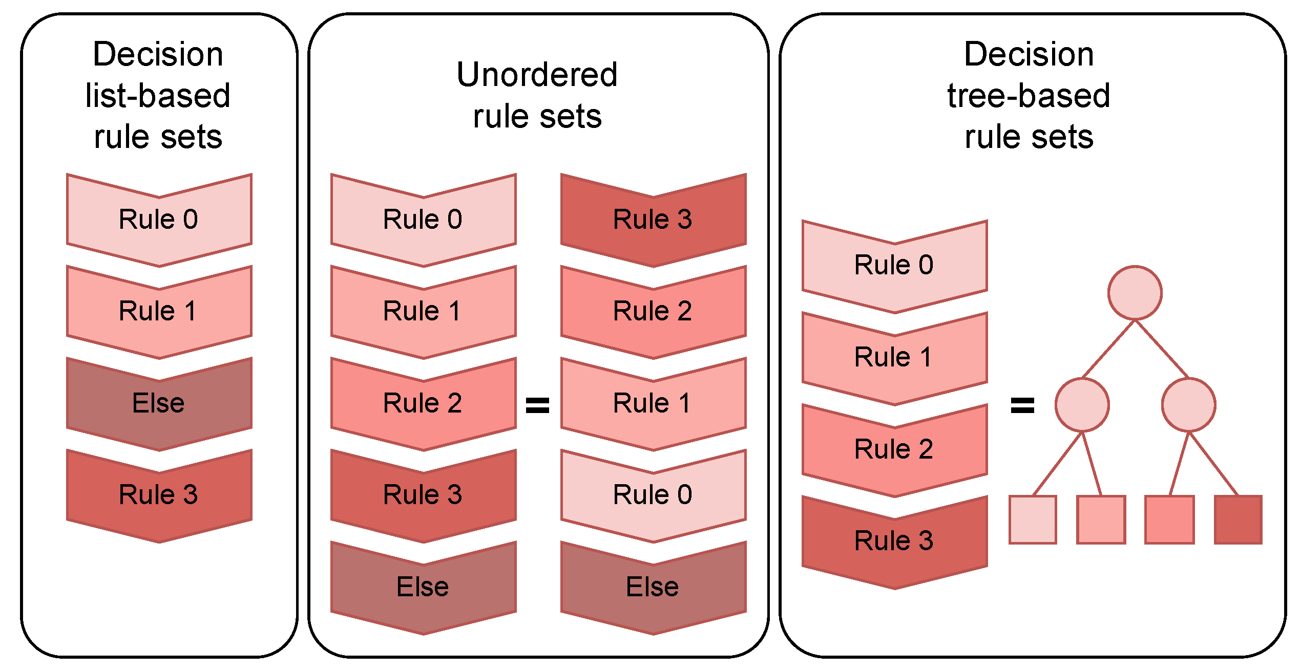
There are three main types of rule sets generated by these methods: DT based, unordered based (the last rule in the rule set is Else), and decision list based. Figure 1 shows the concept of these three types of rule sets. However, previous studies have not provided a metric to distinguish and compare these different rule sets. Therefore, even if an existing metric such as the number of rules suggests a method’s superiority in terms of interpretability, its practical interpretability may remain low. As existing studies have not properly assessed the superiority of the proposed method, a new metric is needed to fill this gap. Table 1 shows the existing interpretability metrics for rule sets.
In the present study, we propose an interpretability metric, Complexity of Rules with Empirical Probability (), to allow for comparisons of interpretability between different rule sets. enables a fair comparison of different types of rule sets, such as decision list- and DT-based rule sets. We also explore the interpretability of the rules generated by the tree ensemble approximators. Specifically, we present and compare not only objective metrics, but also rule sets generated by the tree ensemble approximators and the Recursive-Rule eXtraction algorithm (Re-RX) with J48graft [32].
The contributions of this study are as follows:
- 1.
- Introduction of a New Interpretability Metric: We propose a metric designed to evaluate and compare the interpretability of different types of rule sets. This metric addresses the gap in quantitative assessments of the interpretability of rule sets.
- 2.
- Comparative Analysis of Rule Sets: We provide an exhaustive comparison of decision list- and DT-based rule sets generated by the tree ensemble approximator. Our analysis provides new insights into the strengths and weaknesses of each type of rule set. Furthermore, we explain why categorical and numerical attributes should be treated separately.
- 3.
- Focus on the Interpretability of Categorical and Numerical Attributes: We explain the necessity of separating categorical and numerical attributes. This focus addresses a significant gap in current research as many existing methods overlook the distinction between categorical and numerical attributes.
2. Related Work
The Re-RX algorithm [31] is a rule-based approach that can handle categorical and numerical attributes separately and extract rules recursively. By separating categorical and numerical attributes, Re-RX can generate rules that are intuitively easy to understand. Re-RX with J48graft [32] is the extended version of Re-RX. Numerous studies have conducted research on Re-RX [44,45,46,47,48,49]. RuleFit [33] is a method that employs a linear regression model with a DT-based model to utilize interactions. The rules generated by the ensemble tree are used as new features and fitted using Lasso linear regression. inTrees [34] extracts, measures, prunes, and selects rules from tree ensembles such as RFs and boosts trees to generate a simplified tree ensemble learner for interpretable predictions. DefragTrees [35] involves simplifying complex tree ensembles, such as RFs, to enhance interpretability by formulating the simplification as a model selection problem and employing a Bayesian algorithm that optimizes the simplified model while preserving prediction performance. Initially introduced for independent tree ensembles by Sagi and Rokach [36], Forest-based Trees (FBTs) were later extended to dependent tree ensembles. Combined within both bagging (e.g., RFs) and boosting ensembles (e.g., GBMs), FBTs construct a singular DT from an ensemble of trees. Rule COmbination and SImplification (RuleCOSI+) [39], a recent advance in the field, is a fast post-hoc explainability approach. In contrast to its precursor, RuleCOSI, which was limited to imbalanced data and Adaboost-based small trees according to Obregon et al. [38], RuleCOSI+ was designed as an algorithm that extends the capabilities of RuleCOSI to function effectively in both bagging (e.g., RFs) and boosting (e.g., GBMs) ensembles. DefragTrees, FBTs, and Re-RX generate DT-based rule sets, inTree generates an unordered-based rule set, and RuleCOSI+ generates a decision list-based rule set.
Given this background, in the present study, we aim to provide new insights into the reasons why DL-based and DL-inspired classifiers do not work well for categorical datasets mainly consisting of nominal attributes [50].
3. Materials and Methods
3.1. Datasets
We used 10 datasets from the University of California, Irvine, Machine Learning Repository [51] to compare each method. We provide the sources of these datasets in Appendix A. The details of the datasets are shown in Table 2. For each dataset, we split the data into training–test at a ratio of 8:2. Consistent splits were applied to all methods, with a unique seed-based split for each iteration. Each iteration means in the -fold cross-validation (CV) scheme described in Section 4.3.
3.2. Baseline
We used scikit-learn’s DT and J48graft [52] as simple DT-based methods. J48graft is a grafted (pruned or unpruned) C4.5 [53] DT. This DT generates a binary tree, while J48graft, capable of handling categorical attributes, generates an m-ary tree.
We used FBTs and RuleCOSI+ for the tree ensemble approximator. Figure 2 and Figure 3 show overviews of FBTs and RuleCOSI+, respectively. Both FBTs and RuleCOSI+ were implemented using the official code provided by the authors (https://github.com/sagyome/XGBoostTreeApproximator (13 March 2024) https://github.com/jobregon1212/rulecosi (13 March 2024).
As a rule-based method, we used Re-RX with J48graft, an overview of which is shown in Figure 4. In Re-RX with J48graft, a method derived from the Re-RX grafting family that incrementally adds rules to form a rule set is conditionally selected. If the accuracy does not significantly increase, it aims to improve interpretability. Re-RX with J48graft and its interpretability are positioned at one end of the spectrum, leading to a smaller model. Thus, for large datasets or more complex ensemble models, Re-RX with J48graft does not consider either tree ensembles or growth strategies for increased tree depth. In learning a multilayer perceptron (MLP) in Re-RX with J48graft, we apply one-hot encoding (we used OneHotEncoder from scikit-learn [54]) to categorical attributes to enable efficient learning. With the application of the one-hot encoding to categorical attributes, we modified the pruning algorithm for the MLP. In the original pruning algorithm, the attributes are removed from when , where represents all weights in the first layer of the MLP connected to the i-th attribute. Let be the set of categorical attributes in the dataset , and be the set of one-hot encoded values for the i-th categorical attribute . In this study, we modified the pruning algorithm as follows: , if , then .
All fitted methods are converted to the RuleSet (https://github.com/jobregon1212/rulecosi/blob/master/rulecosi/rules.py (13 March 2024)) module implemented by Obregon and Jung [39].
4. Proposed Methodology
In this section, we present the methodology of experiments for comparing methods.
4.1. Data Preprocessing
We applied one-hot encoding to the categorical attributes because of the inability of FBTs, RuleCOSI+, and DT to handle categorical attributes. For example, if there is a categorical attribute , it is converted to the new attributes and . For the numeric attributes, we applied standardization only to the training and prediction of the MLP in Re-RX with J48graft.
4.2. Interpretability Metrics
The metrics of interpretability, such as the total number of rules () and average number of conditions, are often used. However, these metrics cannot distinguish between decision list-based, unordered, and DT-based rule sets.
We propose a new interpretability metric, , to facilitate fair comparisons of interpretability between different rule sets. quantifies the complexity of rules based on their empirical probability (coverage on the training data), and is defined as follows:
where is the number of conditions in rule r, and is the coverage of rule r in training data . If the rule set is a decision list or an unordered rule set, the instances in the data refer to one or more rules in the rule set. Taking Figure 1 as an example, the actual rule for an instance classified into Rule 2 () in a decision list-based rule set is . In the unordered rule set, the actual rule for an instance classified into Else is . Therefore, if the rule set is a decision list, is accumulated from the top, and if the rule set is an unordered rule set, the of all rules is added together for the Else rule in the rule set. The operation of accumulation allows to compare different rule sets fairly.
represents the expected value of the number of conditions in the rules using the empirical probability obtained from the training data. In other words, if rules with a high likelihood of being referenced have fewer conditions, decreases, and if they have more conditions, increases. Conversely, rules with a low likelihood of being referenced may have many conditions, but their impact is minimal. Compared with and the average number of conditions, which evaluate the interpretability of the entire model, can be considered a more practical metric.
in Equation (1) treats all classes equally and therefore underestimates the interpretability of minority class rules when the dataset is class-imbalanced. This problem can be solved by calculating for each class. We redefine as follows:
where C is the set of all classes and is the subset for each class in the rule set. micro- is useful for both unbalanced datasets and evaluating entire rule sets. In this paper, we refer to micro- as .
4.3. Model Evaluation and Hyperparameter Optimization
We performed the experiment using a stratified -fold CV (https://scikit-learn.org/stable/modules/generated/sklearn.model_selection.StratifiedKFold.html (13 March 2024)) scheme, which is a 10-fold CV repeated 10 times. In each CV-fold, we performed hyperparameter optimization using Optuna [55]. First, the hyperparameters of the base model, which is an MLP in Re-RX with J48graft and XGBoost in FBTs and RuleCOSI+, were optimized to maximize the classification performance. Then, the other hyperparameters were optimized using multi-objective optimization (https://optuna.readthedocs.io/en/stable/tutorial/20_recipes/002_multi_objective.html (13 March 2024)) to maximize both classification performance and interpretability simultaneously. For both DT and J48graft, the first step was skipped because these methods do not have a base model. We used the area under the receiver operating characteristics curve (AUC-ROC) [56] for the classification performance metric, and the inverse of () for the interpretability metric. See Appendix B for details on the hyperparameters in each method.
In the case of multi-objective optimization, the optimal hyperparameters are provided on the Pareto front. From the Pareto front, we selected the hyperparameters that maximize the following equation:
where is a parameter that controls the trade-off between classification performance and interpretability. This equation indicates that increases by and decreases by half, which are equivalent. A higher prioritizes classification performance, whereas a lower prioritizes interpretability. In this experiment, we set . In other words, the value increasing by four points and decreasing by half are equivalent. We excluded the Pareto solution with . When , the rule set R classifies all instances into the same label, which is a meaningless rule set.
4.4. Summary of Evaluation Schemes for Each CV-Fold
Each CV-fold evaluation scheme of our proposed method is shown in Algorithm 1. First, we preprocess the datasets , , and . Next, using the training dataset , we conduct hyperparameter optimization on the validation dataset . From the Pareto front, we select the optimal hyperparameters using Equation (5). Subsequently, we fit the model to the dataset with the selected hyperparameters and evaluate it on dataset . Finally, we return the score set S for the rule set . By using this scheme, we are able to maximize the performance of each method.
| Algorithm 1 Evaluation scheme for each CV-fold |
Require: Training dataset , Validation dataset , Test dataset , Method M Ensure: The score set S for rule set
|
5. Results
In this section, we present the experimental results and their analyses.
5.1. Classification Results
The classification results are presented in Table 3. RuleCOSI+ outperformed the other methods in many datasets. DT was inferior to RuleCOSI+ but superior to the other baselines. FBTs and J48graft performed better than Re-RX with J48graft, but tended to generate more rules and less interpretability than the other baselines, as discussed in the next subsection. Re-RX with J48graft was inferior to the other baselines on average, but showed competitive results against RuleCOSI+ in some datasets.
5.2. Interpretability Results
The interpretability results and the number of rules in and are presented in Table 4 and Table 5. RuleCOSI+ outperformed the other methods for many datasets in . In particular, the variance was considerably smaller than that of the other methods, resulting in stable rule set generation. On the other hand, was larger than other methods. Because RuleCOSI+ generated a decision list-based rule set, tended to be large. This is discussed in detail in Section 5.4 and Section 6.4. DT obtained superior and for many datasets. FBTs and J48graft produced very large for some datasets. FBTs had higher variance in the tic-tac-toe, german, biodeg, and bank-marketing datasets, indicating unstable rule set generation. Furthermore, was larger for FBTs, even though it is a tree-based method. Although Re-RX with J48graft resulted in being slightly higher than the other methods, except FBTs, on average, was much lower than the other methods. Re-RX with J48graft and J48graft tended to have a large because they both handle categorical attributes.
5.3. Summary of Comparative Experiments
Table 6 shows a summary of all the classification and interpretability results presented in the previous subsections. RuleCOSI+ had the highest scores for and , a result that overwhelmed the other methods when was emphasized as an indicator of interpretability. Although DT and Re-RX with J48graft were inferior to RuleCOSI+ in terms of classification performance, they outperformed the other methods in . In other words, DT and Re-RX with J48graft are appropriate when the interpretability and classification frequency of the rules by which instances are classified are important. FBTs and J48graft were not significantly better than the other methods in any of the metrics, and were relatively unsuitable when interpretability was more important.
5.4. Two Examples
We present two examples of rules actually generated in the german and bank-marketing datasets and compare DT, Re-RX with J48graft, and RuleCOSI+. We excluded FBTs and J48graft from the comparison in this section because of the relatively large numbers of rules and the difficulty of analyzing the rules. For each method, rules with matching the median were adopted.
In RuleCOSI+ and DT, categorical attributes were renamed into columns by one-hot encoding. For example, the one-hot encoding for element a of attribute x generates the attribute x =“a”. In other words, a rule such as is equivalent to , and a rule such as is equivalent to . To maintain consistency in notation, we converted all one-hot encoded categorical attributes in the rules to the format or .
5.4.1. bank-marketing
Table 7 shows an example of the rule set generated by each method. The rule set generated by RuleCOSI+ consists of complex rules involving both numerical and categorical attributes. Furthermore, the rule for class 1 had extremely low interpretability because it was expressed as follows:
By contrast, the rule set generated by Re-RX with J48graft consists exclusively of rules based on categorical attributes, resulting in a relatively high interpretability. Furthermore, it is simplified by post-processing, as shown in Table 8. The rule set generated by DT, while containing numerical attributes, was composed of simple rules.
5.4.2. german
Table 9 shows an example of the rule set generated by each method. As in Section 5.4.1, the rule set generated by RuleCOSI+ contained a complex mixture of numerical and categorical attributes, and the rule for class 1 was Equation (6), which had extremely low interpretability. On the other hand, the rule set generated by Re-RX with J48graft was relatively highly interpretable because the rules were composed of categorical attributes, except for and . For and , Re-RX with J48graft performed subdivision and added the numerical attribute duration to improve the accuracy of the rule for 0<=X<200. Also, as shown in Table 10, the rule set can be simpler, as in Section 5.4.1. The rule set generated by DT, while containing numerical attributes, was composed of simple rules.
6. Discussion
6.1. Why Should We Avoid a Mixture of Categorical and Numerical Attributes?
Many methods that have been proposed to enhance interpretability cannot handle categorical and numerical attributes separately. If we could adequately express a rule using only categorical attributes, the use of numerical attributes would reduce interpretability. The conditions for categorical attributes are easy to understand intuitively because they are categorized into a finite group. On the other hand, the conditions for numerical attributes are difficult to understand intuitively because there are an infinite number of thresholds, so the division is not deterministic. Furthermore, it is not common for the division to be performed convincingly. For example, in the german dataset, there are only four conditions for the attribute checking_status ∈ {no checking, <0, 0<=X<200, >=200}, whereas the conditions for the attribute are infinite. In the division of the condition 10,841.5 in in RuleCOSI+ in Table 9, it is difficult to understand why the value 10,841.5 was chosen. Furthermore, rules that contain many numerical attribute conditions make it more difficult to understand how each condition relates to the other. Setting thresholds for numerical attributes is infinite, and an intuitive understanding of how such thresholds affect the other attributes and the overall rules is difficult. Combining the conditions of multiple numerical attributes exponentially increases the complexity of the rule. By contrast, the conditions for categorical attributes are clustered in a finite group, which makes their relationships and effects easier to understand. Therefore, to realize high interpretability, mixing categorical and numerical attributes should be avoided.
6.2. Optimal Selection of the Pareto Solutions
In this study, we selected the Pareto optimal solution from the Pareto front obtained by multi-objective optimization with Optuna using Equation (5). However, the Pareto optimal solution selected by Equation (5) is not always the optimal solution sought by the user. As shown in Figure 5, we observed that the Pareto front depends significantly on the dataset, method, and data splitting. In other words, to select the optimal Pareto solution in real-world applications, it is desirable to verify the Pareto front individually.
6.3. Decision Lists vs. Decision Trees
DTs delineate distinct, nonoverlapping regions within the training data, which affects the depth of the tree when representing complex regions. Conversely, decision lists are superior to DTs in that they allow overlapped regions in the feature space to be represented by different rules, thereby generating more concise rule descriptions for decision boundaries for the classification problem.
On the other hand, when interpreting rules corresponding to an instance, DTs only require tracing the node corresponding to the instance, whereas decision lists require concatenating rules until the instance is classified, which makes the rules more complex. In other words, even if the apparent size of the decision list is small, such as and the average number of conditions, it is actually a very complex rule set with less interpretability than DTs. Therefore, if interpretability is important, DTs or DT-based rule sets are the better choice.
6.4. as a Metric of Interpretability
measures the complexity of a rule set based on empirical probabilities and is an intuitive metric of the interpretability of the rule set. can be used to compare the interpretability of both decision list- and DT-based rule sets because it is calculated separately for these models. RuleCOSI+, which is a decision list-based rule set that was concluded to have low interpretability in Section 5.4.1 and Section 5.4.2, has a high value compared with the other methods in Table 5, showing that the examples and the indicator are consistent. From the above, we can conclude that is an appropriate metric for evaluating the interpretability of rule sets.
6.5. Limitations
In this study, all datasets were used for the evaluation of binary classification. We found the Pareto optimal solution from the Pareto front obtained by multi-objective optimization using Equation (5), but this equation is specialized for binary classification. In multi-class classification, effective results were not obtained using Equation (5). For example, a solution in which there are no rules corresponding to a certain class was sometimes selected as the best solution. To solve this issue, it will be necessary to devise an equation which is specialized for multi-class classification.
Furthermore, it is important to recognize that the size of the datasets used in this study was small to medium. The computational complexity of RuleCOSI+ and FBTs increases exponentially with the size of the data and the number of attributes. This is primarily due to the greedy algorithms employed in these methods. It was not practical to conduct experiments on large datasets within a reasonable time frame; therefore, while comparisons between tree ensembles and Re-RX with J48graft were possible, further validation is needed to provide conclusive evidence for the effectiveness of on broader datasets. Such an attempt would improve our understanding of not only the metric’s applicability, but also its generalizability across different domains and data types beyond those categorically addressed in this study.
7. Conclusions
In the present study, we compared the tree ensemble approximator with Re-RX with J48graft and showed the importance of handling categorical and numerical attributes separately. RuleCOSI+ obtained a high interpretability on the measure with a small number of rules. However, the rules that are actually used to classify instances are complex and have quite a low interpretability. On the other hand, Re-RX with J48graft obtained a low interpretability on the measure with a large number of rules. However, it can handle categorical and numerical attributes separately, has simple rules, and achieves high interpretability, even when the number of rules is large. We newly proposed as a metric for interpretability, which is based on the empirical probability of the rules and measures their complexity. can be used for a fair comparison of decision list- and DT-based rule sets. Furthermore, by using macro- in Equation (4), interpretability can be evaluated appropriately, even for class-imbalanced datasets. Few studies have considered handling categorical and numerical attributes separately, and we believe that this is an important issue for future work. Existing tree ensembles do not distinguish between categorical and numerical attributes because they prioritize accuracy. Therefore, they cannot be distinguished by tree ensemble approximators such as RuleCOSI+ and FBTs. In the future, we plan to develop a tree ensemble that distinguishes categorical from numeric attributes and serves as an approximator with even better interpretability.
Author Contributions
Conceptualization, S.O. and Y.H.; methodology, S.O.; software, S.O., M.N. and R.F.; validation, S.O.; formal analysis, S.O.; investigation, S.O.; resources, S.O.; data curation, S.O., M.N. and R.F.; writing—original draft preparation, S.O.; writing—review and editing, S.O., M.N., R.F. and Y.H.; visualization, S.O.; supervision, Y.H.; project administration, S.O.; funding acquisition, Y.H. All authors have read and agreed to the published version of the manuscript.
Funding
This research received no external funding.
Data Availability Statement
All data were presented in the main text. The source code is available at https://github.com/somaonishi/InterpretableML-Comparisons (13 March 2024).
Acknowledgments
We sincerely thank the reviewer and editor for supporting our research in all aspects based on their expertise and for their help in preparing the manuscript.
Conflicts of Interest
The authors declare no conflicts of interest.
Appendix A. Dataset Sources
The sources of the datasets used in the experiments are listed in Table A1. We used the OpenML-Python package [58] to obtain the datasets. Only the occupancy data were directly obtained from the UCI repository. We utilized the datatraining.txt file for our experiments.

Table A1.
Dataset OpenML id and UCI link.
| Dataset | ID | URL |
|---|---|---|
| heart | 53 | https://archive.ics.uci.edu/dataset/145/statlog+heart (13 March 2024) |
| australian | 40981 | https://archive.ics.uci.edu/dataset/143/statlog+australian+credit+approval (13 March 2024) |
| mammographic | 45557 | https://archive.ics.uci.edu/dataset/161/mammographic+mass (13 March 2024) |
| tic-tac-toe | 50 | https://archive.ics.uci.edu/dataset/101/tic+tac+toe+endgame (13 March 2024) |
| german | 44096 | https://archive.ics.uci.edu/dataset/144/statlog+german+credit+data (13 March 2024) |
| biodeg | 1494 | https://archive.ics.uci.edu/dataset/254/qsar+biodegradation (13 March 2024) |
| banknote | 1462 | https://archive.ics.uci.edu/dataset/267/banknote+authentication (13 March 2024) |
| bank-marketing | 1558 | https://archive.ics.uci.edu/dataset/222/bank+marketing (13 March 2024) |
| spambase | 44 | https://archive.ics.uci.edu/dataset/94/spambase (13 March 2024) |
| occupancy | - | https://archive.ics.uci.edu/dataset/357/occupancy+detection (13 March 2024) |
Appendix B. Implementation Details and Hyperparameters
In this section, we provide the implementation details and hyperparameters for each method. See our repository (https://github.com/somaonishi/InterpretableML-Comparisons (13 March 2024)) for more details.
Appendix B.1. XGBoost
Implementation. We used XGBoost (https://xgboost.readthedocs.io/en/stable/python/python_api.html#xgboost.XGBClassifier (13 March 2024)) for the base tree ensemble for FBTs and RuleCOSI+. We fixed and did not tune the following hyperparameters:
In Table A2, we provide the hyperparameter space.
Table A2.
XGBoost hyperparameter space.
| Parameter | Space |
|---|---|
| UniformInt (1, 10) | |
| LogUniform (1 × 10−4,1.0) | |
| # Iterations | 50 |
Appendix B.2. FBTs
Implementation. We used the official implementation of FBTs (https://github.com/sagyome/XGBoostTreeApproximator (13 March 2024)). We fixed and did not tune the following hyperparameters:
In Table A3, we provide the hyperparameter space.
Table A3.
FBTs hyperparameter space.
| Parameter | Space |
|---|---|
| UniformInt (1, 10) | |
| {auc, None} | |
| # Iterations | 50 |
Appendix B.3. RuleCOSI+
Implementation. We used the official implementation of RuleCOSI+ (https://github.com/jobregon1212/rulecosi (13 March 2024)). In Table A4, we provide the hyperparameter space.
Table A4.
RuleCOSI+ hyperparameter space.
| Parameter | Space |
|---|---|
| Uniform (0.0, 0.95) | |
| Uniform (0.0, 0.5) | |
| c | Uniform (0.1, 0.5) |
| # Iterations | 50 |
Appendix B.4. Re-RX with J48graft
Implementation. We used the repository (https://github.com/somaonishi/rerx (13 March 2024)) that we implemented for Re-RX with J48graft. We used , where d is the amount of training data. In addition, we fixed and did not tune the following hyperparameters in the MLP:
- [59]
In Table A5, we provide the hyperparameter space of the MLP. We searched for the optimal parameters of the MLP and then the other parameters of Re-RX with J48graft. In Table A6, we provide the hyperparameter space for the other parameters of Re-RX with J48graft.
Table A5.
MLP hyperparameter space.
| Parameter | Space |
|---|---|
| UniformInt (1, 5) | |
| LogUniform (5 × 10⁻³, 0.1) | |
| LogUniform (1 × 10⁻⁶, 1 × 10⁻²) | |
| # Iterations | 50 |
Table A6.
Re-RX with J48graft hyperparameter space.
| Parameter | Space |
|---|---|
| {2, 4, 8, …, 128} | |
| Uniform (0.1, 0.5) | |
| LogUniform (0.001, 0.25) | |
| Uniform (0.05, 0.4) | |
| Uniform (0.05, 0.4) | |
| # Iterations | 50 |
Appendix B.5. DT
Implementation. We used scikit-learn’s DT (https://scikit-learn.org/stable/modules/generated/sklearn.tree.DecisionTreeClassifier.html (13 March 2024)). In Table A7, we provide the hyperparameter space. We used the default hyperparameters of scikit-learn for the other parameters.
Table A7.
DT hyperparameter space.
| Parameter | Space |
|---|---|
| UniformInt (1, 10) | |
| Uniform (0.0, 0.5) | |
| Uniform (0.0, 0.5) | |
| # Iterations | 100 |
Appendix B.6. J48graft
Implementation. We used J48graft as implemented in the rerx repository (https://github.com/somaonishi/rerx/blob/main/rerx/tree/tree.py (13 March 2024)). Table A8 shows the hyperparameter space.
Table A8.
J48graft hyperparameter space.
| Parameter | Space |
|---|---|
| {2, 4, 8, …, 128} | |
| Uniform (0.1, 0.5) | |
| # Iterations | 100 |
Appendix C. Results for Other Metrics
Table A9.
Results for the average number of conditions.
| Dataset | FBTs | RuleCOSI+ | Re-RX with J48graft | J48graft | DT |
|---|---|---|---|---|---|
| heart | |||||
| australian | |||||
| mammographic | |||||
| tic-tac-toe | |||||
| german | |||||
| biodeg | |||||
| banknote | |||||
| bank-marketing | |||||
| spambase | |||||
| occupancy | |||||
| ranking | 4.0 | 2.1 | 2.5 | 4.1 | 2.3 |
Table A10.
Results for precision.
| Dataset | FBTs | RuleCOSI+ | Re-RX with J48graft | J48graft | DT |
|---|---|---|---|---|---|
| heart | |||||
| australian | |||||
| mammographic | |||||
| tic-tac-toe | |||||
| german | |||||
| biodeg | |||||
| banknote | |||||
| bank-marketing | |||||
| spambase | |||||
| occupancy | |||||
| ranking | 2.8 | 3.3 | 3.3 | 2.5 | 3.1 |
Table A11.
Results for recall.
| Dataset | FBTs | RuleCOSI+ | Re-RX with J48graft | J48graft | DT |
|---|---|---|---|---|---|
| heart | |||||
| australian | |||||
| mammographic | |||||
| tic-tac-toe | |||||
| german | |||||
| biodeg | |||||
| banknote | |||||
| bank-marketing | |||||
| spambase | |||||
| occupancy | |||||
| ranking | 2.9 | 1.1 | 3.9 | 3.8 | 3.0 |
Table A12.
Results for F1-score.
| Dataset | FBTs | RuleCOSI+ | Re-RX with J48graft | J48graft | DT |
|---|---|---|---|---|---|
| heart | |||||
| australian | |||||
| mammographic | |||||
| tic-tac-toe | |||||
| german | |||||
| biodeg | |||||
| banknote | |||||
| bank-marketing | |||||
| spambase | |||||
| occupancy | |||||
| ranking | 3.0 | 2.1 | 4.0 | 3.0 | 2.9 |
References
- Saeed, W.; Omlin, C. Explainable AI (XAI): A systematic meta-survey of current challenges and future opportunities. Knowl. Based Syst. 2023, 263, 110273. [Google Scholar] [CrossRef]
- Barredo Arrieta, A.; Díaz-Rodríguez, N.; Del Ser, J.; Bennetot, A.; Tabik, S.; Barbado, A.; Garcia, S.; Gil-Lopez, S.; Molina, D.; Benjamins, R.; et al. Explainable Artificial Intelligence (XAI): Concepts, taxonomies, opportunities and challenges toward responsible AI. Inf. Fusion 2020, 58, 82–115. [Google Scholar] [CrossRef]
- Adadi, A.; Berrada, M. Peeking Inside the Black-Box: A Survey on Explainable Artificial Intelligence (XAI). IEEE Access 2018, 6, 52138–52160. [Google Scholar] [CrossRef]
- Zhang, Y.; Tiňo, P.; Leonardis, A.; Tang, K. A Survey on Neural Network Interpretability. IEEE Trans. Emerg. Top Comput. Intell. 2021, 5, 726–742. [Google Scholar] [CrossRef]
- Demajo, L.M.; Vella, V.; Dingli, A. Explainable AI for Interpretable Credit Scoring. In Computer Science & Information Technology (CS & IT); AIRCC Publishing Corporation: Chennai, India, 2020. [Google Scholar] [CrossRef]
- Petch, J.; Di, S.; Nelson, W. Opening the Black Box: The Promise and Limitations of Explainable Machine Learning in Cardiology. Can. J. Cardiol. 2022, 38, 204–213. [Google Scholar] [CrossRef]
- Weber, L.; Lapuschkin, S.; Binder, A.; Samek, W. Beyond explaining: Opportunities and challenges of XAI-based model improvement. Inf. Fusion 2023, 92, 154–176. [Google Scholar] [CrossRef]
- Vilone, G.; Longo, L. Classification of Explainable Artificial Intelligence Methods through Their Output Formats. Mach. Learn. Knowl. Extr. 2021, 3, 615–661. [Google Scholar] [CrossRef]
- Cabitza, F.; Campagner, A.; Malgieri, G.; Natali, C.; Schneeberger, D.; Stoeger, K.; Holzinger, A. Quod erat demonstrandum?—Towards a typology of the concept of explanation for the design of explainable AI. Expert Syst. Appl. 2023, 213, 118888. [Google Scholar] [CrossRef]
- Deck, L.; Schoeffer, J.; De-Arteaga, M.; Kühl, N. A Critical Survey on Fairness Benefits of XAI. arXiv 2023. [Google Scholar] [CrossRef]
- Breiman, L. Bagging predictors. Mach. Learn. 1996, 24, 123–140. [Google Scholar] [CrossRef]
- Breiman, L. Random forests. Mach. Learn. 2001, 45, 5–32. [Google Scholar] [CrossRef]
- Mason, L.; Baxter, J.; Bartlett, P.; Frean, M. Boosting Algorithms as Gradient Descent. In Advances in Neural Information Processing Systems; Solla, S., Leen, T., Müller, K., Eds.; MIT Press: Cambridge, MA, USA, 1999; Volume 12. [Google Scholar]
- Chen, T.; Guestrin, C. XGBoost: A Scalable Tree Boosting System. In Proceedings of the KDD ’16: 22nd ACM SIGKDD International Conference on Knowledge Discovery and Data Mining, San Francisco, CA, USA, 13–17 August 2016; pp. 785–794. [Google Scholar] [CrossRef]
- Ke, G.; Meng, Q.; Finley, T.; Wang, T.; Chen, W.; Ma, W.; Ye, Q.; Liu, T.Y. LightGBM: A Highly Efficient Gradient Boosting Decision Tree. In Proceedings of the 31st International Conference on Neural Information Processing Systems, Red Hook, NY, USA, 4–9 December 2017; NIPS’17. pp. 3149–3157. [Google Scholar]
- Prokhorenkova, L.; Gusev, G.; Vorobev, A.; Dorogush, A.V.; Gulin, A. CatBoost: Unbiased boosting with categorical features. arXiv 2019. [Google Scholar] [CrossRef]
- Sagi, O.; Rokach, L. Ensemble learning: A survey. WIREs Data Min. Knowl. Discov. 2018, 8, e1249. [Google Scholar] [CrossRef]
- Rudin, C. Stop explaining black box machine learning models for high stakes decisions and use interpretable models instead. Nat. Mach. Intell. 2019, 1, 206–215. [Google Scholar] [CrossRef]
- Longo, L.; Brcic, M.; Cabitza, F.; Choi, J.; Confalonieri, R.; Ser, J.D.; Guidotti, R.; Hayashi, Y.; Herrera, F.; Holzinger, A.; et al. Explainable Artificial Intelligence (XAI) 2.0: A manifesto of open challenges and interdisciplinary research directions. Inf. Fusion 2024, 106, 102301. [Google Scholar] [CrossRef]
- Zihni, E.; Madai, V.I.; Livne, M.; Galinovic, I.; Khalil, A.A.; Fiebach, J.B.; Frey, D. Opening the black box of artificial intelligence for clinical decision support: A study predicting stroke outcome. PLoS ONE 2020, 15, e0231166. [Google Scholar] [CrossRef]
- Yang, C.C. Explainable Artificial Intelligence for Predictive Modeling in Healthcare. J. Healthc. Inform. Res. 2022, 6, 228–239. [Google Scholar] [CrossRef]
- Carmona, P.; Dwekat, A.; Mardawi, Z. No more black boxes! Explaining the predictions of a machine learning XGBoost classifier algorithm in business failure. Res. Int. Bus. Financ. 2022, 61, 101649. [Google Scholar] [CrossRef]
- Lipton, Z.C. The Mythos of Model Interpretability. arXiv 2017. [Google Scholar] [CrossRef]
- Qian, H.; Ma, P.; Gao, S.; Song, Y. Soft reordering one-dimensional convolutional neural network for credit scoring. Knowl. Based Syst. 2023, 266, 110414. [Google Scholar] [CrossRef]
- Mahbooba, B.; Timilsina, M.; Sahal, R.; Serrano, M. Explainable artificial intelligence (XAI) to enhance trust management in intrusion detection systems using decision tree model. Complexity 2021, 2021, 6634811. [Google Scholar] [CrossRef]
- Shulman, E.; Wolf, L. Meta Decision Trees for Explainable Recommendation Systems. In Proceedings of the AIES ’20: AAAI/ACM Conference on AI, Ethics, and Society, New York, NY, USA, 7–9 February 2020; pp. 365–371. [Google Scholar] [CrossRef]
- Blanco-Justicia, A.; Domingo-Ferrer, J.; Martínez, S.; Sánchez, D. Machine learning explainability via microaggregation and shallow decision trees. Knowl. Based Syst. 2020, 194, 105532. [Google Scholar] [CrossRef]
- Sachan, S.; Yang, J.B.; Xu, D.L.; Benavides, D.E.; Li, Y. An explainable AI decision-support-system to automate loan underwriting. Expert Syst. Appl. 2020, 144, 113100. [Google Scholar] [CrossRef]
- Yang, L.H.; Liu, J.; Ye, F.F.; Wang, Y.M.; Nugent, C.; Wang, H.; Martinez, L. Highly explainable cumulative belief rule-based system with effective rule-base modeling and inference scheme. Knowl. Based Syst. 2022, 240, 107805. [Google Scholar] [CrossRef]
- Li, H.; Wang, Y.; Zhang, S.; Song, Y.; Qu, H. KG4Vis: A Knowledge Graph-Based Approach for Visualization Recommendation. IEEE Trans. Vis. Comput. Graph. 2022, 28, 195–205. [Google Scholar] [CrossRef]
- Setiono, R.; Baesens, B.; Mues, C. Recursive Neural Network Rule Extraction for Data With Mixed Attributes. IEEE Trans. Neural Netw. 2008, 19, 299–307. [Google Scholar] [CrossRef] [PubMed]
- Hayashi, Y.; Nakano, S. Use of a Recursive-Rule eXtraction algorithm with J48graft to achieve highly accurate and concise rule extraction from a large breast cancer dataset. Inform. Med. Unlocked 2015, 1, 9–16. [Google Scholar] [CrossRef]
- Friedman, J.H.; Popescu, B.E. Predictive learning via rule ensembles. Ann. Appl. Stat. 2008, 2, 916–954. [Google Scholar] [CrossRef]
- Deng, H. Interpreting tree ensembles with inTrees. Int. J. Data Sci. Anal. 2019, 7, 277–287. [Google Scholar] [CrossRef]
- Hara, S.; Hayashi, K. Making Tree Ensembles Interpretable: A Bayesian Model Selection Approach. In Proceedings of the Twenty-First International Conference on Artificial Intelligence and Statistics, Playa Blanca, Spain, 9–11 April 2018; Volume 84, pp. 77–85. [Google Scholar]
- Sagi, O.; Rokach, L. Explainable decision forest: Transforming a decision forest into an interpretable tree. Inf. Fusion 2020, 61, 124–138. [Google Scholar] [CrossRef]
- Sagi, O.; Rokach, L. Approximating XGBoost with an interpretable decision tree. Inf. Sci. 2021, 572, 522–542. [Google Scholar] [CrossRef]
- Obregon, J.; Kim, A.; Jung, J.Y. RuleCOSI: Combination and simplification of production rules from boosted decision trees for imbalanced classification. Expert Syst. Appl. 2019, 126, 64–82. [Google Scholar] [CrossRef]
- Obregon, J.; Jung, J.Y. RuleCOSI+: Rule extraction for interpreting classification tree ensembles. Inf. Fusion 2023, 89, 355–381. [Google Scholar] [CrossRef]
- Nauck, D.D. Measuring interpretability in rule-based classification systems. In Proceedings of the 12th IEEE International Conference on Fuzzy Systems, FUZZ’03, St. Louis, MO, USA, 25–28 May 2003; IEEE: Piscataway, NJ, USA, 2003; Volume 1, pp. 196–201. [Google Scholar]
- Lakkaraju, H.; Bach, S.H.; Leskovec, J. Interpretable decision sets: A joint framework for description and prediction. In Proceedings of the 22nd ACM SIGKDD International Conference on Knowledge Discovery and Data Mining, San Francisco, CA, USA, 13–17 August 2016; pp. 1675–1684. [Google Scholar]
- Souza, V.F.; Cicalese, F.; Laber, E.; Molinaro, M. Decisiont Trees with Short Explainable Rules. In Advances in Neural Information Processing Systems; Koyejo, S., Mohamed, S., Agarwal, A., Belgrave, D., Cho, K., Oh, A., Eds.; lCurran Associates, Inc.: Red Hook, NY, USA, 2022; Volume 35, pp. 12365–12379. [Google Scholar]
- Margot, V.; Luta, G. A New Method to Compare the Interpretability of Rule-Based Algorithms. AI 2021, 2, 621–635. [Google Scholar] [CrossRef]
- Hayashi, Y. Synergy effects between grafting and subdivision in Re-RX with J48graft for the diagnosis of thyroid disease. Knowl. Based Syst. 2017, 131, 170–182. [Google Scholar] [CrossRef]
- Hayashi, Y.; Oishi, T. High accuracy-priority rule extraction for reconciling accuracy and interpretability in credit scoring. New Gener. Comput. 2018, 36, 393–418. [Google Scholar] [CrossRef]
- Chakraborty, M.; Biswas, S.K.; Purkayastha, B. Recursive Rule Extraction from NN using Reverse Engineering Technique. New Gener. Comput. 2018, 36, 119–142. [Google Scholar] [CrossRef]
- Hayashi, Y. Neural network rule extraction by a new ensemble concept and its theoretical and historical background: A review. Int. J. Comput. Intell. Appl. 2013, 12, 1340006. [Google Scholar] [CrossRef]
- Hayashi, Y. Application of a rule extraction algorithm family based on the Re-RX algorithm to financial credit risk assessment from a Pareto optimal perspective. Oper. Res. Perspect. 2016, 3, 32–42. [Google Scholar] [CrossRef]
- Hayashi, Y.; Takano, N. One-Dimensional Convolutional Neural Networks with Feature Selection for Highly Concise Rule Extraction from Credit Scoring Datasets with Heterogeneous Attributes. Electronics 2020, 9, 1318. [Google Scholar] [CrossRef]
- Hayashi, Y. Does Deep Learning Work Well for Categorical Datasets with Mainly Nominal Attributes? Electronics 2020, 9, 1966. [Google Scholar] [CrossRef]
- Kelly, M.; Longjohn, R.; Nottingham, K. UCI Machine Learning Repository. Available online: https://archive.ics.uci.edu (accessed on 13 March 2024).
- Webb, G.I. Decision Tree Grafting from the All-Tests-but-One Partition. In Proceedings of the IJCAI’99: 16th International Joint Conference on Artificial Intelligence, San Francisco, CA, USA, 31 July–6 August 1999; Volume 2, pp. 702–707. [Google Scholar]
- Quinlan, J.R. C4.5: Programs for Machine Learning; Morgan Kaufmann: Burlington, MA, USA, 1993. [Google Scholar]
- Pedregosa, F.; Varoquaux, G.; Gramfort, A.; Michel, V.; Thirion, B.; Grisel, O.; Blondel, M.; Prettenhofer, P.; Weiss, R.; Dubourg, V.; et al. Scikit-learn: Machine Learning in Python. J. Mach. Learn. Res. 2011, 12, 2825–2830. [Google Scholar]
- Akiba, T.; Sano, S.; Yanase, T.; Ohta, T.; Koyama, M. Optuna: A Next-generation Hyperparameter Optimization Framework. In Proceedings of the 25th ACM SIGKDD International Conference on Knowledge Discovery and Data Mining, Anchorage, AK, USA, 4–8 August 2019. [Google Scholar]
- Bradley, A.P. The use of the area under the ROC curve in the evaluation of machine learning algorithms. Pattern Recognit. 1997, 30, 1145–1159. [Google Scholar] [CrossRef]
- Welch, B. The generalization of students problem when several different population variances are involved. Biometrika 1947, 34, 28–35. [Google Scholar] [CrossRef] [PubMed]
- Feurer, M.; van Rijn, J.N.; Kadra, A.; Gijsbers, P.; Mallik, N.; Ravi, S.; Müller, A.; Vanschoren, J.; Hutter, F. OpenML-Python: An extensible Python API for OpenML. J. Mach. Learn. Res. 2021, 22, 1–5. [Google Scholar]
- Loshchilov, I.; Hutter, F. Decoupled Weight Decay Regularization. In Proceedings of the International Conference on Learning Representations, New Orleans, LA, USA, 6–9 May 2019. [Google Scholar]
Figure 1.
Concepts of the three types of rule sets. Decision list-based rule sets classify instances by sequentially referencing rules from top to bottom. Unordered rule sets classify instances by referencing rules in any order. Decision tree-based rule sets are variable according to decision trees and differ from the other two types of rule sets in that all instances are classified using only a single rule.

Figure 2.
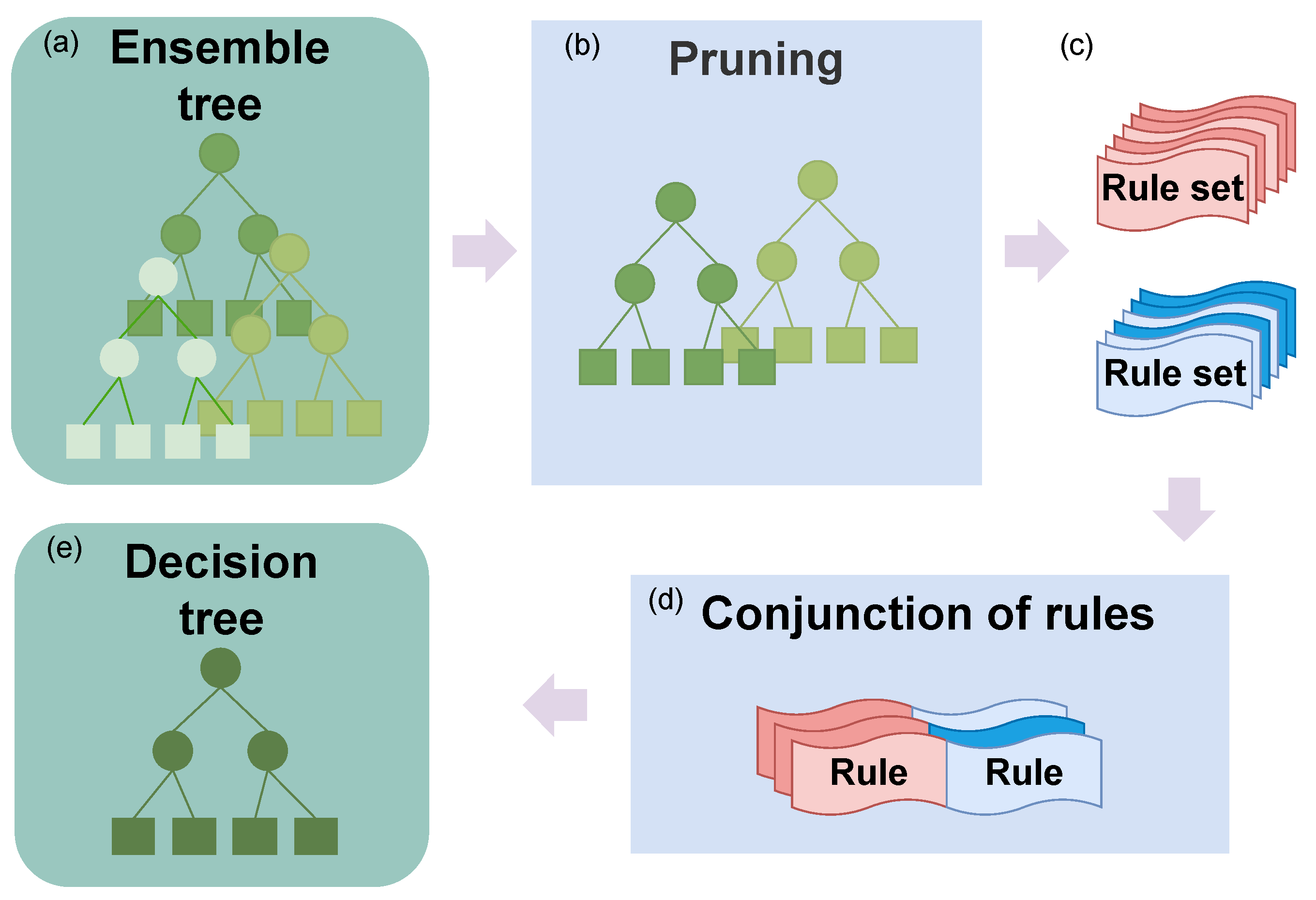
Overview of FBTs. (a) Fit the ensemble tree; (b) pruning: remove trees that do not improve the accuracy from the ensemble tree; (c) convert the tree to rules; (d) conjunction of rules: generate the conjunction set by gradually merging the conjunction sets of the base trees into a single set that represents the entire ensemble; (e) convert to a decision tree.
Figure 2.
Overview of FBTs. (a) Fit the ensemble tree; (b) pruning: remove trees that do not improve the accuracy from the ensemble tree; (c) convert the tree to rules; (d) conjunction of rules: generate the conjunction set by gradually merging the conjunction sets of the base trees into a single set that represents the entire ensemble; (e) convert to a decision tree.

Figure 3.
Overview of RuleCOSI+. (a) Fit the ensemble tree; (b) convert the tree to rule sets; (c) combine rule sets: greedily verify all combinations and determine the rules to adopt and create a new rule set; (d) sequential covering pruning: simplify the rule set; (e) generalize rule set: remove any unnecessary conditions; (f) repeat (c–e) using the rule set generated in (e) and the rule set obtained from the remaining ensemble tree (green rule set in the figure); (g) obtain the final rule set.

Figure 4.
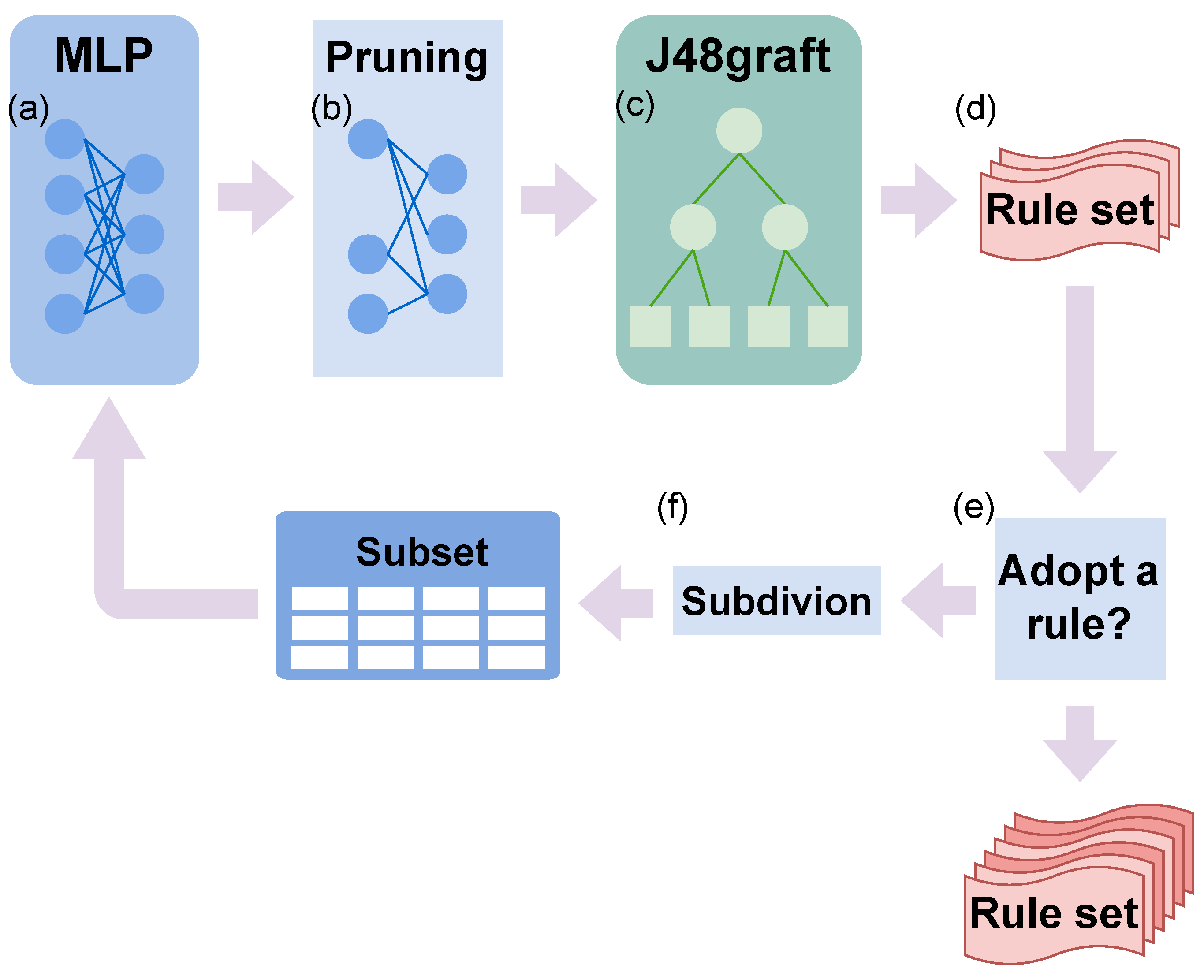
Overview of Re-RX with J48graft. (a) Fit a multilayer perceptron; (b) pruning: reduce the number of attributes; (c) fit J48graft; (d) convert the tree to a rule set; (e) adopt a rule: select a rule to adopt as is; (f) subdivision: recursive (a–e) for a rule that is not adopted using data and has attributes not included in the rule.
Figure 4.
Overview of Re-RX with J48graft. (a) Fit a multilayer perceptron; (b) pruning: reduce the number of attributes; (c) fit J48graft; (d) convert the tree to a rule set; (e) adopt a rule: select a rule to adopt as is; (f) subdivision: recursive (a–e) for a rule that is not adopted using data and has attributes not included in the rule.

Figure 5.
The Pareto fronts for each method obtained by multi-objective optimization using Optuna with seed = 1 and CV-fold = 1, 2, 3 in the german (a–c) and bank-marketing (d–f) datasets.
Figure 5.
The Pareto fronts for each method obtained by multi-objective optimization using Optuna with seed = 1 and CV-fold = 1, 2, 3 in the german (a–c) and bank-marketing (d–f) datasets.

Table 1.
Interpretability metrics for rule sets.
| Metrics | Description |
|---|---|
| Number of rules | This metric is the total number of rules. |
| Number of conditions | This metric is the sum of the total or average number of conditions. |
| Complexity [40] | This metric relates the complexity, namely the number of conditions, to the number of classes. |
| Fraction uncover [41] | This metric measures the proportion of data points covered by at least one rule in the rule set. |
| Fraction overlap [41] | This metric calculates the degree to which rules in the rule set redundantly cover the same data points. |
| Uniq [39] | This metric quantifies the amount of non-redundant conditions contained in the rule set. |
| [42] | This metric is the weighted sum of the number of different attributes, based on the coverage of each rule. |
| Weighted sum of predictivity, stability, and simplicity [43] | This metric combines three critical aspects: predictivity, which assesses accuracy; stability, gauged through the Dice–Sorensen index comparing rule sets; and simplicity, measured by rule length sum, into a comprehensive weighted sum. |
Table 2.
Dataset properties. In this paper, # indicates quantity.
| Dataset | #Instances | #Features | #Cate | #Cont | Major Class Ratio |
|---|---|---|---|---|---|
| heart | 270 | 13 | 7 | 6 | 0.55 |
| australian | 690 | 14 | 6 | 8 | 0.555 |
| mammographic | 831 | 4 | 2 | 2 | 0.52 |
| tic-tac-toe | 958 | 9 | 9 | 0 | 0.65 |
| german | 1000 | 20 | 7 | 13 | 0.70 |
| biodeg | 1055 | 41 | 0 | 41 | 0.66 |
| banknote | 1372 | 4 | 0 | 4 | 0.55 |
| bank-marketing | 4521 | 16 | 9 | 7 | 0.89 |
| spambase | 4601 | 57 | 0 | 57 | 0.60 |
| occupancy | 8143 | 5 | 0 | 5 | 0.79 |
Table 3.
Results for classification performance (). All metrics are reported as . In this paper, for each dataset, the top results are in bold (here, “top” means that the gap between this result and the result with the best score is not statistically significant at a level of 0.05 (Welch’s t-test [57])). For each dataset, ranks are calculated by sorting the average of the reported scores, and the “rank” row reports the average rank across all datasets.
| Dataset | FBTs | RuleCOSI+ | Re-RX with J48graft | J48graft | DT |
|---|---|---|---|---|---|
| heart | |||||
| australian | |||||
| mammographic | |||||
| tic-tac-toe | |||||
| german | |||||
| biodeg | |||||
| banknote | |||||
| bank-marketing | |||||
| spambase | |||||
| occupancy | |||||
| ranking | 2.9 | 2.1 | 4.0 | 3.2 | 2.8 |
Table 4.
Results for the number of rules.
| Dataset | FBTs | RuleCOSI+ | Re-RX with J48graft | J48graft | DT |
|---|---|---|---|---|---|
| heart | |||||
| australian | |||||
| mammographic | |||||
| tic-tac-toe | |||||
| german | |||||
| biodeg | |||||
| banknote | |||||
| bank-marketing | |||||
| spambase | |||||
| occupancy | |||||
| ranking | 4.5 | 1.6 | 3.3 | 3.8 | 1.8 |
Table 5.
Results for CREP.
| Dataset | FBTs | RuleCOSI+ | Re-RX with J48graft | J48graft | DT |
|---|---|---|---|---|---|
| heart | |||||
| australian | |||||
| mammographic | |||||
| tic-tac-toe | |||||
| german | |||||
| biodeg | |||||
| banknote | |||||
| bank-marketing | |||||
| spambase | |||||
| occupancy | |||||
| ranking | 3.5 | 4.7 | 1.5 | 3.1 | 2.2 |
Table 6.
Summary of classification and interpretability performance () across all datasets. For each metric, the top results are in bold (here, “top” means that the gap between this result and the result with the best score is not statistically significant at a level of 0.05 (Welch’s t-test [57])).
Table 6.
Summary of classification and interpretability performance () across all datasets. For each metric, the top results are in bold (here, “top” means that the gap between this result and the result with the best score is not statistically significant at a level of 0.05 (Welch’s t-test [57])).
| Method | |||
|---|---|---|---|
| FBTs | |||
| RuleCOSI+ | |||
| Re-RX with J48graft | |||
| J48graft | |||
| DT |
Table 7.
Rule sets generated from the bank-marketing dataset.
| RuleCOSI+ | Coverage | |
| 0.744 | ||
| 0.148 | ||
| 0.109 | ||
| Re-RX with J48graft | Coverage | |
| 0.820 | ||
| 0.108 | ||
| 0.044 | ||
| 0.0 | ||
| 0.029 | ||
| DT | Coverage | |
| 0.891 | ||
| 0.025 | ||
| 0.084 |
Table 8.
Post-processed rule set generated from the bank-marketing dataset in Re-RX with J48graft.
| Re-RX with J48graft | Coverage | |
| 0.971 | ||
| 0.0 | ||
| 0.029 |
Table 9.
Rule sets generated from the german dataset.
| RuleCOSI+ | Coverage | |
| 0.329 | ||
| 0.283 | ||
| 0.388 | ||
| Re-RX with J48graft | Coverage | |
| 0.394 | ||
| 0.063 | ||
| 0.16 | ||
| 0.067 | ||
| 0.013 | ||
| 0.022 | ||
| 0.012 | ||
| 0.19 | ||
| 0.079 | ||
| DT | Coverage | |
| 0.394 | ||
| 0.325 | ||
| 0.281 |
Table 10.
Post-processed rule set generated from the german dataset in Re-RX with J48graft.
| Re-RX with J48graft | Coverage | |
| 0.394 | ||
| 0.063 | ||
| 0.067 | ||
| 0.207 | ||
| 0.19 | ||
| 0.079 |
Disclaimer/Publisher’s Note: The statements, opinions and data contained in all publications are solely those of the individual author(s) and contributor(s) and not of MDPI and/or the editor(s). MDPI and/or the editor(s) disclaim responsibility for any injury to people or property resulting from any ideas, methods, instructions or products referred to in the content. |
© 2024 by the authors. Licensee MDPI, Basel, Switzerland. This article is an open access article distributed under the terms and conditions of the Creative Commons Attribution (CC BY) license (https://creativecommons.org/licenses/by/4.0/).
Share and Cite
MDPI and ACS Style
Onishi, S.; Nishimura, M.; Fujimura, R.; Hayashi, Y. Why Do Tree Ensemble Approximators Not Outperform the Recursive-Rule eXtraction Algorithm? Mach. Learn. Knowl. Extr. 2024, 6, 658-678. https://doi.org/10.3390/make6010031
AMA Style
Onishi S, Nishimura M, Fujimura R, Hayashi Y. Why Do Tree Ensemble Approximators Not Outperform the Recursive-Rule eXtraction Algorithm? Machine Learning and Knowledge Extraction. 2024; 6(1):658-678. https://doi.org/10.3390/make6010031
Chicago/Turabian StyleOnishi, Soma, Masahiro Nishimura, Ryota Fujimura, and Yoichi Hayashi. 2024. "Why Do Tree Ensemble Approximators Not Outperform the Recursive-Rule eXtraction Algorithm?" Machine Learning and Knowledge Extraction 6, no. 1: 658-678. https://doi.org/10.3390/make6010031