A Probabilistic Transformation of Distance-Based Outliers

Abstract

The scores of distance-based outlier detection methods are difficult to interpret, and it is challenging to determine a suitable cut-off threshold between normal and outlier data points without additional context. We describe a generic transformation of distance-based outlier scores into interpretable, probabilistic estimates. The transformation is ranking-stable and increases the contrast between normal and outlier data points. Determining distance relationships between data points is necessary to identify the nearest-neighbor relationships in the data, yet most of the computed distances are typically discarded. We show that the distances to other data points can be used to model distance probability distributions and, subsequently, use the distributions to turn distance-based outlier scores into outlier probabilities. Over a variety of tabular and image benchmark datasets, we show that the probabilistic transformation does not impact outlier ranking (ROC AUC) or detection performance (AP, F1), and increases the contrast between normal and outlier score distributions (statistical distance). The experimental findings indicate that it is possible to transform distance-based outlier scores into interpretable probabilities with increased contrast between normal and outlier samples. Our work generalizes to a wide range of distance-based outlier detection methods, and, because existing distance computations are used, it adds no significant computational overhead.

1. Introduction

We propose a generic method to transform the scores of distance-based outlier detection methods into interpretable, probabilistic estimates. An outlier is often described as “an observation (or subset of observations) which appears to be inconsistent with the remainder of that set of data” [1]. The definition of an inconsistent observation depends on the application and algorithm used. Ruff et al. [2] define an inconsistent observation as “an observation that deviates considerably from some concept of normality”, but an inconsistent observation can also be defined as an object that stems from a different distribution from the model describing the data, as in the classical definition of Hawkins [3]: “An outlier is an observation which deviates so much from the other observations as to arouse suspicions that it was generated by a different mechanism”. An outlier is also referred to as an anomaly or novelty, sometimes interchangeably. Therefore, outlier detection is also referred to as anomaly detection or novelty detection. Because the methods used to detect outliers, anomalies, and novelties are mostly the same, we make no distinction between these terms and refer to inconsistent instances as outliers. Outlier detection is a broad research field that includes probabilistic approaches such as classical density estimation, clustering approaches to determine outliers, one-class classification methods, reconstruction-based methods, or generative approaches; for a detailed overview, refer to one of the extensive reviews [2,4,5,6,7,8]. In a distance-based setting, we can define outliers as objects located far away from the remaining objects.

Notation
${\displaystyle a}$	A scalar (integer or real)
${\displaystyle \mathit{a}}$	A vector
${\displaystyle \mathit{A}}$	A matrix
${\displaystyle \mathrm{a}}$	A scalar random variable
${\displaystyle \mathbb{A}}$	A set
${\displaystyle \mathcal{A}}$	A space
${\displaystyle A}$	A distribution
${\displaystyle \mathbb{R}}$	The set of real numbers
${\displaystyle \mathbb{X}}$	A dataset
${\displaystyle \{0,1,\dots ,n\}}$	The set of all integers between 0 and n
${\displaystyle f\left(x\right):\mathbb{A}\to \mathbb{B}}$	A function of x with domain $\mathbb{A}$ and range $\mathbb{B}$

Specifically, given a metric space $(\mathcal{M},d)$ with metric d, each object $\mathit{x}\in \mathcal{M}$ receives a real-valued outlier score $s:=q\left(\mathit{x}\right)$ via a function $q:\mathcal{M}\to \mathbb{R}$, where the function depends on the distances to the other objects in the dataset. To determine if an observation is considered an outlier, it is necessary to establish a threshold value by converting outlier scores into binary labels of normal and outlier data points. A major challenge in distance-based outlier detection is the interpretation of the resulting scores. The scores provided by distance-based methods differ widely in their scale, range, and meaning. Even when considering only a single outlier detection method, the same outlier score can describe different degrees of outlierness depending on the kind of data. These challenges make the interpretation and comparison of outlier scores difficult. Distance-based outlier detection scores are typically derived from neighborhood representation given a distance matrix. We propose that the information contained in the distance matrix can be used to derive a probabilistic normalization set that can be used to transform outlier scores into outlier probabilities. Based on a large number of benchmark datasets, we test our approach in terms of detection performance and interpretability and show that it is possible to achieve interpretable, probabilistic outlier scores with no detriment to the resulting detection performance. The rest of this paper is organized as follows: Section 2 provides an overview of distance-based outlier detection methods. In Section 3, we show outlier score normalization schemes and their application to distance-based methods. In Section 4, we describe our proposed probabilistic normalization scheme, and in Section 5, we describe the results of applying our scheme on benchmark datasets. Finally, in Section 6, we derive conclusions and provide opportunities for future research.

2. Distance-Based Outlier Detection

In this section, we introduce and review common distance-based outlier detection methods and formalize them as a scoring function $q:\mathcal{M}\to \mathbb{R}$ on a metric space $(\mathcal{M},d)$, such that an outlier detection method assigns a real-valued outlier score to an observation. We further differentiate between the closed-world and open-world outlier detection setting, an often disregarded yet highly relevant aspect of distance-based outlier detection. The following outlier detection methods are formulated in a closed-world setting, such that the observations in a dataset $\mathbb{X}$ are assigned an outlier score. Often, however, it is necessary to assign an outlier score to unseen data, such that a model of normality is determined based on a dataset $\mathbb{X}$, and the outlier score is determined on unseen observations in a dataset ${\mathbb{X}}_{\mathrm{test}}$. At the end of this section, we provide a simple approach to transfer said closed-world outlier detection methods into an open-world setting.

2.1. Nearest Neighbors

Knorr et al. [9,10,11] first formalized a distanced-based notion of outliers in which an object $\mathit{x}\in \mathbb{X}$ is said to be a DB-outlier in a dataset of n objects if $\left|\{{\mathit{x}}^{\prime }\in \mathbb{X}\mid d(\mathit{x},{\mathit{x}}^{\prime })>\delta \}\right|\ge \alpha n$, where $\alpha ,\delta \in \mathbb{R}$ are parameters to be specified by the user and $0\le \alpha \le 1$. In this specification, a fraction $\alpha$ of all objects have a distance from $\mathit{x}$ that is larger than $\delta$. Chandola et al. [7] point out that this method can be viewed as global density estimation for each instance since it involves counting the number of neighbors in a hypersphere of radius $\delta$. However, a major drawback of this definition is that it is difficult to determine a distance threshold $\delta$ and the results do not determine a ranking of scores.

Ramaswamy et al. [12] build upon the ideas presented for DB-outliers. To determine the outlier score of an instance, they propose the use of the distance to its $k^{\mathrm{th}}$ nearest neighbor as a score; thus, we refer to the method as $k^{\mathrm{th}}\mathrm{NN}$. Compared to DB-outliers, the main benefit of this approach is that it does not require the user to specify a distance $\delta$. The $k^{\mathrm{th}}\mathrm{NN}$ outlier score of an observation $\mathit{x}$ is defined as

$$q_{k^{\mathrm{th}}\mathrm{NN}}\left(\mathit{x}\right):=d^{\left(k\right)}(\mathit{x},\mathbb{X})$$

(1)

where $\mathit{x}\in \mathbb{X}$ and $d^{\left(k\right)}(\mathit{x},\mathbb{X})$ are the distance between $\mathit{x}$ and its $k^{\mathrm{th}}$ nearest neighbor in $\mathbb{X}$.

Angiulli and Pizzuti [13] adapt the $k^{\mathrm{th}}\mathrm{NN}$ approach to use the average distance to the k-nearest neighbors of a point $\mathit{x}$ instead of the $k^{\mathrm{th}}$ distance, which can also be interpreted as the maximum distance. We refer to this method as $k\mathrm{NN}$ and define it as follows:

$$q_{k\mathrm{NN}}\left(\mathit{x}\right):=\frac{1}{k}\sum _{i=1}^k{d}^{\left(i\right)}(\mathit{x},\mathbb{X})$$

(2)

where $\mathit{x}\in \mathbb{X}$ and $d^{\left(i\right)}(\mathit{x},\mathbb{X})$ are the distance between $\mathit{x}$ and its $i^{\mathrm{th}}$ nearest neighbor in $\mathbb{X}$.

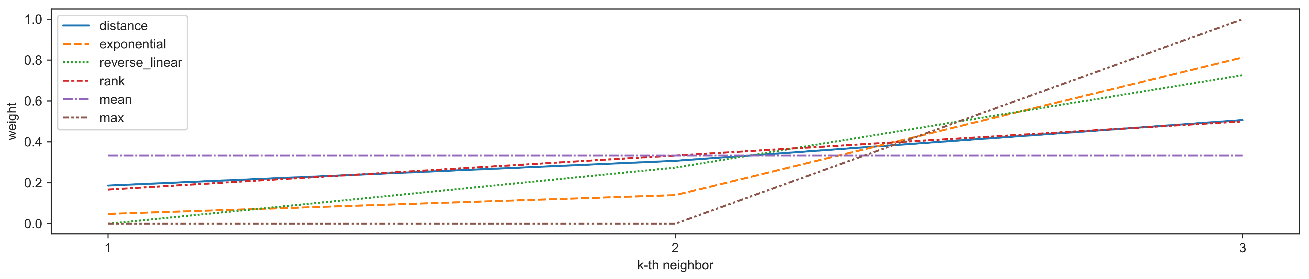
We propose a generalization of $k^{\mathrm{th}}\mathrm{NN}$ and $k\mathrm{NN}$ as specific instances of weighting schemes for distance-based outlier detection. Weighting schemes are commonly used in k-nearest neighbor classification, where the schemes traditionally emphasize close neighbors and disregard neighbors farther away [14]. However, as evident in $k^{\mathrm{th}}\mathrm{NN}$-based outlier detection, where only the farthest neighbor is considered, we propose emphasizing the neighbors farther away. A further difference between weighted classification and weighted outlier detection is the predicted result, which corresponds to class votes or outlier scores. To keep the resulting outlier scores in the same range, we propose sum-normalizing the weights such that the resulting weight vectors sum to one. The resulting outlier scores can subsequently be interpreted as a (smoothened) distance. We adapt some of the weighting measures investigated in Geler et al. [14] to the outlier detection task and describe $k^{\mathrm{th}}\mathrm{NN}$ as max-weighted and $k\mathrm{NN}$ as mean-weighted outlier detection. The distance and rank schemes are adapted from Dudani’s weighted nearest-neighbor classification [15], the exponential scheme from Zavrel [16], and the linear scheme from Macleod et al. [17]. In all cases, we reverse the schemes such that the farthest neighbor receives the largest weight. We define the schemes for a vector of k-nearest neighbor distances $\mathit{d}$ as follows

$$\begin{array}{cc}\hfill {\mathit{w}}_{max}\left(\mathit{d}\right)& =[0,0,\dots ,1]\hfill \end{array}$$

(3)

$$\begin{array}{cc}\hfill {\mathit{w}}_{\mathrm{mean}}\left(\mathit{d}\right)& =\left[\frac{1}{k},\frac{1}{k},\dots ,\frac{1}{k}\right]\hfill \end{array}$$

(4)

$$\begin{array}{cc}\hfill {\mathit{w}}_{\mathrm{distance}}(\mathit{d},s)& =[d_1^s,d_2^s,\dots ,d_n^s]\hfill \end{array}$$

(5)

$$\begin{array}{cc}\hfill {\mathit{w}}_{\mathrm{exponential}}(\mathit{d},a,b)& =[exp\left(a{d}_1^b\right),exp\left(a{d}_2^b\right),\dots ,exp\left(a{d}_n^b\right)]\hfill \end{array}$$

(6)

$$\begin{array}{cc}\hfill {\mathit{w}}_{\mathrm{linear}}\left(\mathit{d}\right)& =[\mathrm{scale}(d_1,\mathit{d}),\mathrm{scale}(d_2,\mathit{d}),\dots ,\mathrm{scale}(d_n,\mathit{d})]\hfill \end{array}$$

(7)

$$\begin{array}{cc}\hfill {\mathit{w}}_{\mathrm{rank}}\left(\mathit{d}\right)& =[1,2,\dots ,k]\hfill \end{array}$$

(8)

where ${\mathit{w}}_{max}$ is 1 only if $d_i=max\left(\mathit{d}\right)$; s, a, and b are real-valued hyperparameters of the respective weighting schemes; and the linear scaling function is defined as

$$\mathrm{scale}(x,\mathit{d})=\frac{x-min\left(\mathit{d}\right)}{max\left(\mathit{d}\right)-min\left(\mathit{d}\right)}.$$

(9)

We show how the weights influence the determination of an outlier score based on a three-nearest-neighbors example in Figure 1. Since the weighting schemes are not the primary focus of our work, we use fixed hyperparameters $s=a=b=1$; thus, ${\mathit{w}}_{\mathrm{distance}}\left(\mathit{d}\right)=[d_1,d_2,\dots ,d_n]$ and ${\mathit{w}}_{\mathrm{exponential}}\left(\mathit{d}\right)=[exp\left(d_1\right),exp\left(d_2\right),\dots ,exp\left(d_n\right)]$ for the purpose of our work.

Because outlier scores are assumed to be positive values derived from distances, sum-normalization is possible by dividing each element in the weight vector by its sum as defined in Equation (10). Sum-normalization ensures that the weight vector sums to one and the weighted outlier score can be interpreted as a weighted distance. We further use the proposed weighting scheme to define a generic weighted k-nearest neighbor approach ($\mathrm{kNNW}$), which serves as a basis for our tabular outlier detection experiments in Section 5.

$$q_{\mathrm{kNNW}}\left(\mathit{x}\right):=\frac{\mathit{d}·\mathit{w}}{{\sum }_{i=1}^k{w}_i}$$

(10)

where $\mathit{d}$ is the vector of k-nearest neighbor distances, $\mathit{w}$ is the k-dimensional weight vector, and · denotes the dot product between the distance and weight vectors.

More recently, authors proposed various sampling schemes to improve the efficiency of the described techniques. Wu and Jermaine [18] propose an iterative sampling scheme to approximate the result of the $k^{\mathrm{th}}\mathrm{NN}$ detector described in Equation (1), which we designate as the $k^{\mathrm{th}}$ iteratively sampled nearest neighbor ($k^{\mathrm{th}}\mathrm{ISNN}$).

$$q_{k^{\mathrm{th}}\mathrm{ISNN}}\left(\mathit{x}\right):=d^{\left(k\right)}(\mathit{x},S_{\mathit{x}}\left(\mathbb{X}\right))$$

(11)

where $S_{\mathit{x}}\left(\mathbb{X}\right)$ is a randomly sampled subset of $\mathbb{X}$ excluding $\mathit{x}$, and $d^{\left(k\right)}$ is the distance to the $k^{\mathrm{th}}$ nearest neighbor in $S_{\mathit{x}}\left(\mathbb{X}\right)$. The subsampling is determined individually for each point ${\mathit{x}}^{\prime }$ processed with $q_{k^{\mathrm{th}}\mathrm{ISNN}}\left({\mathit{x}}^{\prime }\right)$; therefore, it is referred to as iterative sampling.

Sugiyama and Borgwardt [19] show that a simplification of $k^{\mathrm{th}}\mathrm{ISNN}$ leads to better detection performance over 16 different datasets. The authors propose removing the iterative aspect of $k^{\mathrm{th}}\mathrm{ISNN}$ and, instead, sample only once for all data points and identify the first nearest neighbor, which we describe as the sampled nearest neighbor ($\mathrm{SNN}$).

$$q_{\mathrm{SNN}}\left(\mathit{x}\right):=\underset{{\mathit{x}}^{\prime }\in S\left(\mathbb{X}\right)}{min}d(\mathit{x},{\mathit{x}}^{\prime })$$

(12)

where $S\left(\mathbb{X}\right)$ is an independent random subset of the data that is determined once and the score is defined as the minimum distance to points in $S\left(\mathbb{X}\right)$. In other words, for a point $\mathit{x}$, this method uses the distance to its closest point ${\mathit{x}}^{\prime }$ in a fixed sample $S\left(\mathbb{X}\right)$ as a score.

Pang et al. [20] extend the $\mathrm{SNN}$ approach by repeatedly sampling random subsets of the data, which we term repeatedly sampled nearest neighbor ($\mathrm{RSNN}$).

$$q_{\mathrm{RSNN}}\left(\mathit{x}\right):=\frac{1}{r}\sum _{i=1}^r\underset{{\mathit{x}}^{\prime }\in S_i\left(\mathbb{X}\right)}{min}d(\mathit{x},{\mathit{x}}^{\prime })$$

(13)

where r is the number of random subsets to the sample and $S_i\left(\mathbb{X}\right)$ is the i-th random sample. This method essentially represents an ensemble of nearest-neighbor outlier detection models and, consequently, improves upon $\mathrm{SNN}$, which the authors empirically show using 11 datasets. It can be argued that k-nearest neighbor ensembles such as a combination of $k^{\mathrm{th}}\mathrm{NN}$ or $k\mathrm{NN}$ detectors with data subsampling are a generalization of $\mathrm{RSNN}$, which are well-known techniques to improve neighbor-based outlier detection [21,22,23].

In addition to data sampling techniques, other authors use randomized sampling to determine feature subspaces as initially motivated by Aggarwal and Yu [24]. Kriegel et al. [25] define a set of reference points based on the concept of shared nearest neighbors. The reference points characterize a subspace hyperplane, and the outlier scores are determined by the Euclidean distance of a point $\mathit{x}$ to the subspace hyperplane, weighted by an indicator function that determines the relevance of a dimension. Agrawal [26] proposes a very similar distance-based subspacing approach. Zhang et al. [27] also use a shared nearest-neighbor reference set to determine subspaces, using an angle-based approach to compute the outlier scores. Trittenbach and Böhm [28] propose a method to determine subspaces that considers the relationship between subspaces. Keller et al. [29] propose determining high-contrast subspaces for outlier detection as a form of data pre-processing. Cabero et al. [30] also determine the subspaces as a data pre-processing step based on archetypal analysis followed by a $k^{\mathrm{th}}\mathrm{NN}$ approach. Some authors combine distance-based outlier detection with dimensionality reduction techniques such as principal component analysis [31] for high-dimensional data. In image-based outlier detection, authors use neural networks to evaluate the neighborhood search in latent spaces describing entire images [32], image sub-features [33], or image patch features [34]. Another option to model distance-based outliers is to use reverse nearest neighbor or natural neighbor relationships. For example, outlier detection using indegree number (ODIN) [35] models the nearest-neighbor relationships as a directed graph and defines the outlier score as the indegree number in the graph such that a low indegree number defines an outlier. Radovanović et al. [36] analyze the concept of hubness, which appears in reverse nearest-neighbor outlier detection, and propose an outlier detection method based on anti-hubs; points that do not occur in the nearest neighbors of any other points. Natural neighbors approaches discard the k-nearest neighbor parameter and instead perform a search over $\lambda$ rounds to identify an appropriate number of neighbors such that a shared neighbor relationship is found [37,38]. A further extension is described by extended nearest-neighbor approaches, which combine the nearest neighbors with reverse nearest neighbors and shared nearest neighbors [39,40].

2.2. Local Outlier Factor

In contrast to the previously described techniques, which are referred to as global outlier detection techniques, the local outlier factor (LOF) [41] model introduces the concept of local outliers. Schubert et al. [42] formalize distance-based outlier detection models such that an outlier score is determined based on some context set, typically the k-nearest neighbors of a point $\mathit{x}$. To compare the resulting outlier scores, another set of points is used, which is referred to as the reference set. Global methods compare the resulting score from the context set to all other points in the the dataset $\mathbb{X}$; thus, the reference set is defined as the entire dataset $\mathbb{X}$. Because the score comparison to all other points is considered global, those methods ignore differences in the local densities of the data. Local methods use a different reference set to compare the scores to, typically, the k-nearest neighbors as in the context set. Local methods convert the distance information from the local neighborhood into some form of density; therefore, the methods are sometimes also referred to as density-based. LOF can be defined as a scoring function

$$q_{\mathrm{LOF}}\left(\mathit{x}\right):=p{\left(\mathit{x}\right)}^{-1}\left({\left|N^{\left(k\right)}\left(\mathit{x}\right)\right|}^{-1}\sum _{{\mathit{x}}^{\prime }\in N^{\left(k\right)}\left(\mathit{x}\right)}p\left({\mathit{x}}^{\prime }\right)\right)$$

(14)

where $N^{\left(k\right)}\left(\mathit{x}\right)$ is the set of k-nearest neighbors of $\mathit{x}$ and p is the local reachability density of $\mathit{x}$ defined as $p\left(\mathit{x}\right):=|N^{\left(k\right)}{\left(\mathit{x}\right)|}^{-1}{\sum }_{{\mathit{x}}^{\prime }\in N^{\left(k\right)}\left(\mathit{x}\right)}max\{d^{\left(k\right)}({\mathit{x}}^{\prime },\mathbb{X}),d(\mathit{x},{\mathit{x}}^{\prime })\}$. Note that $N^{\left(k\right)}\left(\mathit{x}\right)$ includes all objects inside the $k^{\mathrm{th}}$ distance, which can, in the case of a “tie”, be more than k objects. The local reachability density can be seen as an average inverse distance of a point $\mathit{x}$ normalized such that the distance cannot be smaller than the $k^{\mathrm{th}}$ distance. According to the authors, the local reachability density stabilizes and prevents statistical fluctuations, a fact later analyzed in more detail by Schubert et al. [43]. The local outlier factor then compares $p\left(\mathit{x}\right)$, the density of the context set, to the average reachability density of the points in the reference set. If the average reachability density in the reference set is higher than the point density obtained from the context set, then the score of the local outlier factor is above one and considered less normal.

Schubert et al. [42] further propose a simplified version of the local outlier factor where p is the inverse $k^{\mathrm{th}}$ distance $p\left(\mathit{x}\right):=d^{\left(k\right)}{(\mathit{x},\mathbb{X})}^{-1}$, which represents a simpler density estimate compared to the local reachability density in $\mathrm{LOF}$. To better illustrate the general concept of local outlier detection, the simplified local outlier factor ($\mathrm{SLOF}$) can be stated as follows:

$$q_{\mathrm{SLOF}}\left(\mathit{x}\right):=\frac{\underset{{\mathit{x}}^{\prime }\in N^{\left(k\right)}\left(\mathit{x}\right)}{\mathrm{mean}}\left(d^{\left(k\right)}{({\mathit{x}}^{\prime },\mathbb{X})}^{-1}\right)}{d^{\left(k\right)}{(\mathit{x},\mathbb{X})}^{-1}}.$$

(15)

The authors show that many local outlier models can be considered variations of SLOF. For example, the local distance-based outlier factor (LDOF) proposed by Zhang et al. [44] is a variation of the simplified LOF model using an average distance as in $k\mathrm{NN}$ instead of the $k^{\mathrm{th}}$ distance as in $k^{\mathrm{th}}\mathrm{NN}$. Influence Outlierness (INFLO) [45] is another variation of the simplified LOF, which diverges by using a different context set that includes reverse nearest neighbors. Another method that can be seen as an extension of the simplified LOF is Local Outlier Probabilities (LoOP) [46], which adds a probabilistic normalization to $\mathrm{SLOF}$. Many more local outlier detection methods have been described in the literature comprising entire literature reviews [47]. Schubert et al. [43] note that local outlier detection methods can be differentiated using their order of locality, and Goodge et al. [48] show that the methods can be generalized as message-passing algorithms on a nearest-neighbors graph.

2.3. Closed-World and Open-World

Distance-based outlier detection methods are typically defined in a closed-world settings; however, there is an important difference between the closed-world and open-world specifications such that, for two equal points $\mathit{x}\in \mathbb{X}$, ${\mathit{x}}^{\prime }\in {\mathbb{X}}_{\mathrm{test}}$ and $\mathit{x}={\mathit{x}}^{\prime }$, the $k^{\mathrm{th}}$ nearest neighbor in $\mathbb{X}$ is different. In the closed-world or transductive setting, the search for the k-nearest neighbors does not include the searched-for point $\mathit{x}$; in other words, the nearest-neighbors graph does not include self-loops. In the open-world setting, it is not known if ${\mathit{x}}^{\prime }$ is contained in the reference set $\mathbb{X}$, and therefore all points in $\mathbb{X}$ are included in the k-nearest neighbors search. All of the referenced methods are described in a closed-world setting and do not state how to perform inductive outlier detection, yet commonly used toolkits for outlier detection focus on the open-world setting [49,50]. We propose transferring the closed-world setting to the open world such that $k+1$ neighbors are used for $\mathbb{X}$, ignoring the first neighbor, and k neighbors for ${\mathbb{X}}_{\mathrm{test}}$. In Section 4, we describe our method in the transductive, closed-world, and inductive, open-world settings.

3. Outlier Score Normalization

As mentioned in the introduction, the outlier scores resulting from distance-based approaches differ widely in their meaning and are challenging to interpret. In some cases, even within a dataset, the scores for two different observations can denote different degrees of outlierness, depending on disparate local data distributions, a core motivation for local outlier detection methods. Some distance-based methods provide probability estimates, for example [46,51,52,53], but these probabilistic interpretations are a core part of the underlying algorithms and cannot easily be transferred to other algorithmic approaches. Latecki et al. [54] developed an outlier detection model based on local kernel density estimates. Schubert et al. [43] more generally analyze the connection of density-based outlier detection algorithms, such as the local distance-based methods, to kernel density estimation. The authors show that distance-based density estimation is closely related to kernel density estimation and claim that local outlier detection methods use heuristics to determine, perhaps coincidentally, something similar to a statistical kernel for density estimation.

Instead of algorithm-specific probabilistic interpretations, some authors propose outlier score normalization schemes independent of the underlying algorithm. A simple way of bringing outlier scores to a common scale is to apply a linear transformation as defined in Equation (9), such that the minimum score is mapped to 0 and the maximum score is mapped to 1. However, such a min–max scaling approach does not yield a useful probabilistic interpretation. Gao and Tan [55] propose two approaches to model outlier scores as probabilities. In the first approach, they assume that the posterior probabilities follow a logistic sigmoid function. In the second approach, they assume that the outlier scores follow a mixture of exponential and Gaussian distributions. In both cases, the authors propose the use of an expectation–maximization approach to learn the parameters. Kriegel et al. [56] propose the use of the cumulative distribution function of a Gaussian or Gamma distribution to normalize the scores. Additionally, the authors show the usefulness of post-processing techniques to ensure a useful expected value for normal data and to increase the contrast between normal and outlier data points. Bouguessa [57] model outlier scores as a beta mixture distribution to directly identify outlier points from the mixture component with the highest score values. Schubert et al. [58] note that a rank-based normalization can be useful if little knowledge is available about the actual scores and score distributions.

3.1. Interpretability, Explanation, and Trustworthiness

The interpretability of outlier predictions should not be confused with the explanation of outlier detection models or the trustworthiness of predictions; therefore, for the ongoing discussion, we differentiate the terms as follows and describe them in detail following our differentiation.

• Interpretability: the ability to judge the relevance of a prediction.
• Explanation: the ability to explain the reasoning behind a prediction.
• Trustworthiness: the ability to describe the confidence behind a prediction.

Explanation is sometimes also referred to as interpretation, but this kind of interpretation is separate from interpretability. Explanation algorithms reveal how models make decisions, but interpretability refers to the degree to which an intrinsic property of an inference result is understandable to human beings [59]. There is a growing interest in methods for deriving explanations of outliers, that is, “to give the users of some outlier detection method further aid in understanding and evaluating the result with respect to their domain” [60]. Explanations highlight why a specific outlier detection model reaches a particular prediction. A common approach to explain outlier predictions is to compare normal data points and outliers in attribute subspaces in which the given outliers show separability from the normal data [61,62,63]. Other authors derive explanations from statistical models of the normal and outlier data using minimum-distance estimation [64]. The explanation of learning methods and outlier detection methods is discussed extensively in a research field known as Explainable Artificial Intelligence, or XAI [65]. Explanations can uncover the hidden weaknesses of a model, also known as “Clever Hanses” [66]. The Clever Hans Effect occurs when the learned model produces correct predictions based on the “wrong” features, which appears to be a widespread problem in outlier detection [67]. Another critical aspect of outlier detection predictions is trustworthiness. Trustworthiness describes an understanding of when a prediction should or should not be trusted [68,69,70]. To achieve better trustworthiness in outlier detection predictions, ref. [71] propose the use of a Bayesian approach to add probabilistic uncertainty estimates to outlier scores, enabling the detector to assign a confidence score to each prediction, which captures its uncertainty in that prediction.

4. Probabilistic Outlier Scores

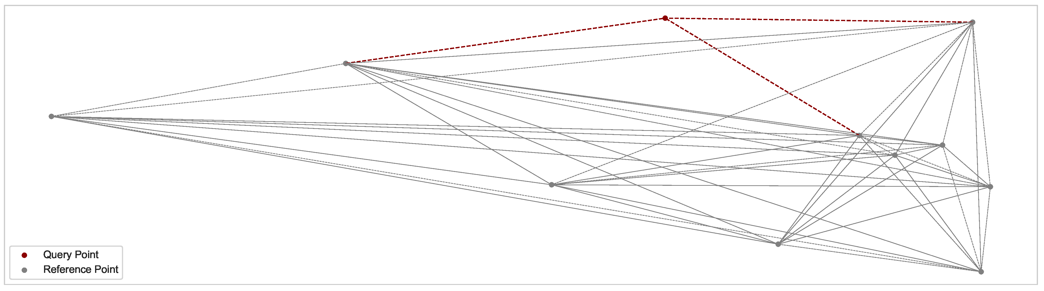
In this section, we derive a generic scheme to transform distance-based outlier detection scores into interpretable outlier scores based on distance probabilities. In the generic score normalization approaches mentioned in Section 3.1, only the actual scores are used for normalization. Conversely, the algorithm-specific normalization schemes are generally not easily transferable to other algorithms. A common theme across a vast majority of distance-based outlier detection methods is the determination of nearest-neighbor relationships between data points. Determining exact nearest-neighbor relationships typically utilizes the computation of all distance relationships between data points, resulting in a distance matrix $\mathit{M}$. Additionally, it has been shown that brute-force distance computation is preferable to index methods except for low-dimensional similarity search problems [72]. We note that approximate nearest-neighbor approaches are also used for distance-based outlier detection strategies [73], but this represents a small minority of methods and is not the focus of our study. In the closed-world setting, the distance matrix corresponds to a square matrix of ${\mathbb{R}}^{n\times n}$ values for n points in the dataset. In the open-world setting, the distance matrix between n reference points ${\mathbb{R}}^{n\times n}$ has to be differentiated from the distance matrix of m query points to n reference points ${\mathbb{R}}^{m\times n}$. For a point ${\mathit{x}}_i$ and a point ${\mathit{x}}_j$, a value in the distance matrix at index $(i,j)$ corresponds to the distance $d({\mathit{x}}_i,{\mathit{x}}_j)$. Most distance-based approaches use the k-nearest neighbors as a context set to determine the outlier score [42], and any probabilistic estimate of those scores would be based on the limited information present in the context set. In contrast to previous approaches, we assume that the additional information contained in the distance matrix is useful for normalization. More concretely, we hypothesize that the additional information can be used to transform outlier scores into interpretable probabilistic estimates. Based on a distance matrix of reference points, we define the concept of a normalization set. A normalization set describes a subset of the distance matrix used for the probabilistic score normalization. In the simplest case, the entire distance matrix is used as a baseline normalization set as shown in Figure 2; hence, the normalization set is defined as the distances contained in the distance matrix $\mathit{M}$ between all reference points excluding self-loops in the matrix diagonal. Additionally, if the distance measure is symmetric, the normalization set from the distance matrix can be reduced to its upper or lower triangular set of values.

We propose using the normalization set to determine a distance probability distribution. For example, in the parametric case, we estimate the parameters of a distribution P based on the distances in the normalization set. The distribution of distances has been investigated in the context of feature similarity [74], hubness reduction [75], local intrinsic dimensionality [76], or compact sets [77]. Pekalska and Duin [78] show, based on the central limit theorem, that distances are approximately normally distributed for independent and identically distributed feature vectors. In general, however, distance distributions seem to differ depending on the characteristics of the input data and we assume that the underlying distance distribution is unknown. Regarding the estimation of distance distributions for outlier detection, we note that the robustness of an estimator should be considered such that an estimator’s breakdown value [79] lies above a possible outlier contamination [80]. Under the assumption that the distances in the normalization set follow an unknown continuous probability distribution, we define a random variable $\mathrm{r}\sim P$ that describes the normalization set. Given a probability density function p on r, any distance $d(\mathit{x},{\mathit{x}}^{\prime })$ can be interpreted as the distance density between $\mathit{x}$ and ${\mathit{x}}^{\prime }$ denoted as $p\left(d(\mathit{x},{\mathit{x}}^{\prime })\right)$ or, in short, $p(\mathit{x},{\mathit{x}}^{\prime })$. The cumulative distance distribution $f(\mathit{x},{\mathit{x}}^{\prime }):=P(\mathrm{r}\le d(\mathit{x},{\mathit{x}}^{\prime }))$ describes the probability of a distance in the normalization set being smaller than or equal to $d(\mathit{x},{\mathit{x}}^{\prime })$. A query point with a distance-based outlier score can be directly interpreted using its distance distribution, where a probability of 99% means that the distance is in the top 1% of distances observed in the normalization set. To estimate an unknown distance distribution, we can use a parametric or non-parametric approach. In the parametric case, we estimate a continuous probability distribution that is expected to fit the data. In the non-parametric case, we can directly use the empirical distribution function or use some other non-parametric estimation method such as robust kernel density estimation [81].

In summary, we hypothesize that it is possible to transform distances to interpretable distance distributions without adverse effects on detection performance. Because a cumulative distribution function is monotonically non-decreasing, the ranking should be stable after the transformation, but due to the limited precision of the computations, it is not guaranteed that the transformation is ranking-stable. To evaluate the impact of our transformation on ranking stability, we use the Receiver Operating Characteristic (ROC) Area Under the Curve (AUC). A perfect ranking results in an ROC AUC value of 1, whereas an inverted perfect ranking would result in a value of 0. A value of $1/2$ can be interpreted as random guessing [82]. Besides ranking stability, we investigate changes to detection performance using average precision (AP) and the popular F1-score, a harmonic mean of precision and recall. Additionally, we evaluate the contrast between normal and outlier scores before and after the transformation using statistical distances. The basis for our experiments are tabular outlier detection benchmark datasets [82,83], and a common image-based benchmark dataset for outlier detection [84,85].

5. Results

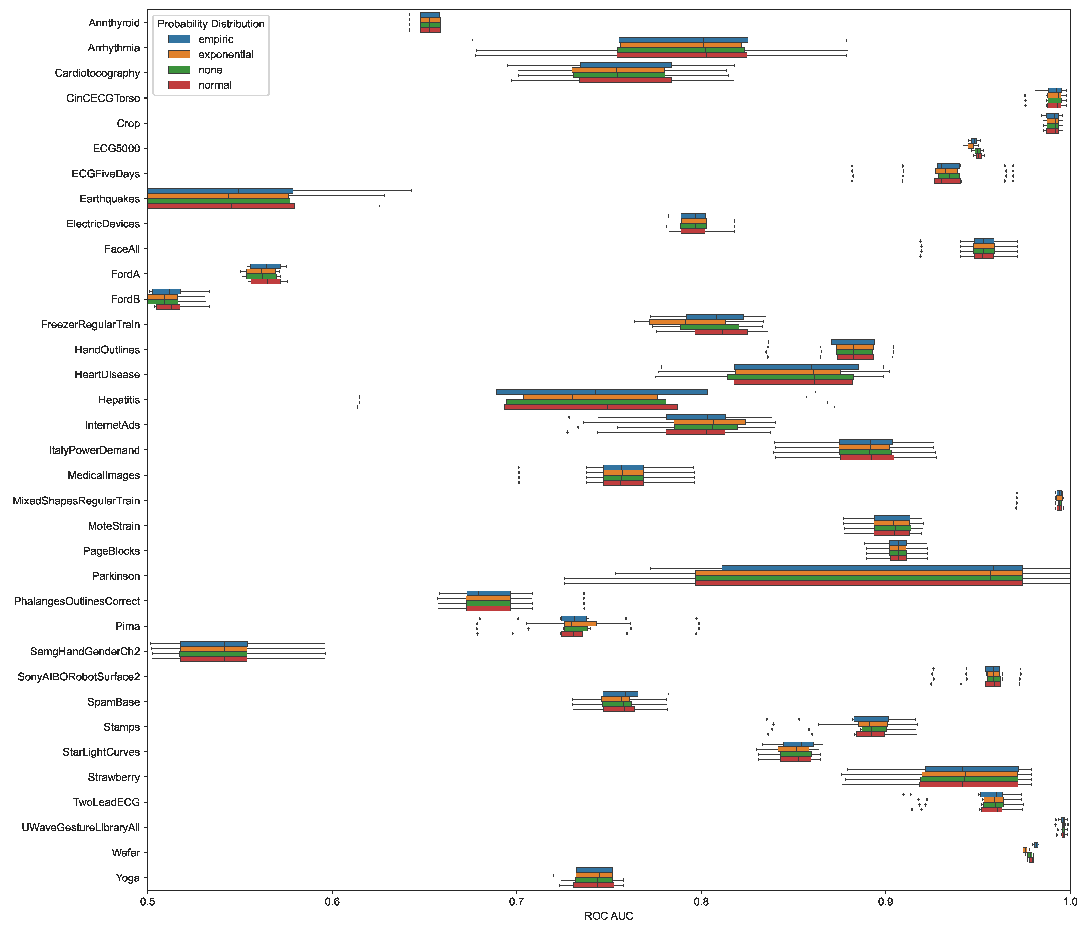
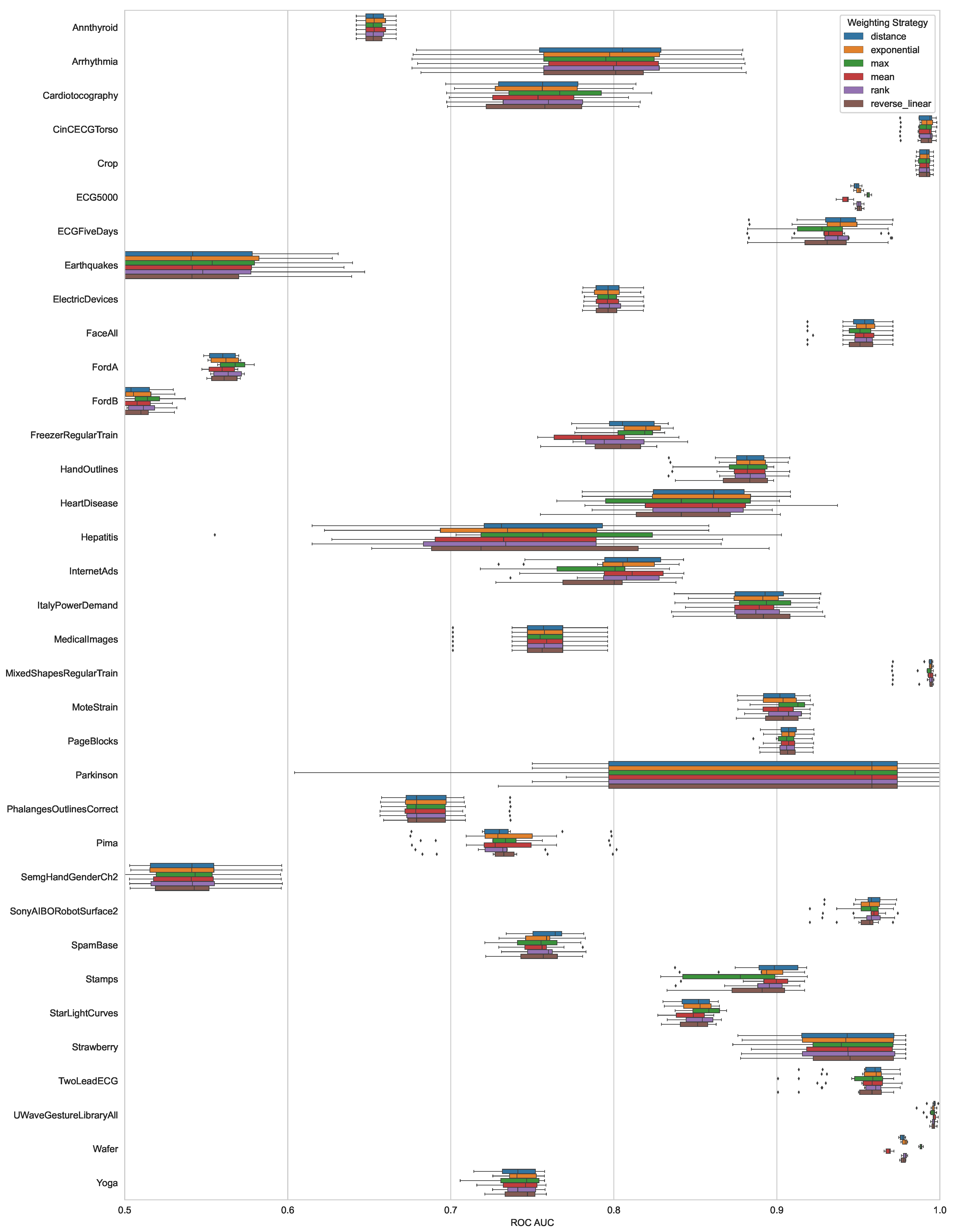
To evaluate the probabilistic transformation on tabular data, we used the proposed weighted k-nearest neighbor approach ($\mathrm{kNNW}$). The datasets used stem from the DAMI [82] library and the UTSD single-concept benchmark [83]. For both dataset collections, we only used the datasets with five percent of outliers, each consisting of ten randomly sampled variants, resulting in the dataset list shown in

Table 1. The datasets used to evaluate the weighted k-nearest neighbors approach ($\mathrm{kNNW}$), where N denotes the number of samples, O the number of outliers, and d the dimensionality.

Dataset	N	O	d	Source	Refs.
Annthyroid	6942	347	21	ELKI	[86]
Arrhythmia	256	12	259	ELKI	[86]
Cardiotocography	1734	86	21	ELKI	[86]
CinCECGTorso	373	18	1639	UTSD	[87]
Crop	1052	52	46	UTSD	[88]
Earthquakes	387	19	512	UTSD	[89]
ECG5000	3072	153	140	UTSD	[87]
ECGFiveDays	465	23	136	UTSD	[89]
ElectricDevices	4500	225	96	UTSD	[89]
FaceAll	344	17	131	UTSD	[89]
FordA	2660	133	500	UTSD	[89]
FordB	2380	119	500	UTSD	[89]
FreezerRegularTrain	1578	78	301	UTSD	[90]
HandOutlines	921	46	2709	UTSD	[91]
HeartDisease	157	7	13	ELKI	[86]
Hepatitis	70	3	19	ELKI	[86]
InternetAds	1682	84	1555	ELKI	[86]
ItalyPowerDemand	575	28	24	UTSD	[92]
MedicalImages	625	31	99	UTSD	[89]
MixedShapesRegularTrain	793	39	1024	UTSD	[93]
MoteStrain	721	36	84	UTSD	[94]
PageBlocks	5139	256	10	ELKI	[86]
Parkinson	50	2	22	ELKI	[86]
PhalangesOutlinesCorrect	1787	89	80	UTSD	[91]
Pima	526	26	8	ELKI	[86]
SemgHandGenderCh2	568	28	1500	UTSD	[95]
SonyAIBORobotSurface2	635	31	65	UTSD	[96]
SpamBase	2661	133	57	ELKI	[86]
Stamps	325	16	9	ELKI	[97]
StarLightCurves	5607	280	1024	UTSD	[98]
Strawberry	369	18	235	UTSD	[89]
TwoLeadECG	611	30	82	UTSD	[87]
UWaveGestureLibraryAll	589	29	945	UTSD	[99]
Wafer	6738	336	152	UTSD	[100]
Yoga	1863	93	426	UTSD	[89]

. For DAMI, we used the normalized and deduplicated variants, and for UTSD, we pre-processed the data points with min–max scaling. We used two-fold, stratified cross-validation to determine an ROC AUC and AP estimate of the resulting distance-based and probabilistic estimates. We used Euclidean distance for all evaluations and fixed the hyperparameters for the weighting schemes as $s=a=b=1$, as shown in Figure 1. For the number of neighbors k of our tested $\mathrm{kNNW}$ method, we picked the best parameter from all possible values of $k\in [1,2,\dots ,100]$. In our first analysis, we investigate the impact of score normalization using different probability distributions. We examine a normal, exponential, and empirical distribution and compare it to the base case where no distribution is used for normalization. To visualize the results of our tabular ranking evaluation, we use box and whisker plots that show the interquartile range (IQR) in a colored area with corresponding whiskers depicting 1.5 IQR and points outside the whiskers drawn individually. In Figure 3, we show that the ROC AUC result after the transformation matches the original result and the transformation is indeed ranking-stable. To analyze the impact on detection performance, we evaluate the mean average precision over all datasets as shown in

Table 2. Mean average precision and corresponding standard deviation over all tabular datasets for $\mathrm{kNNW}$ using different weighting schemes (distance, exponential, max, mean, rank, reverse) and different probabilistic transformations (empiric, exponential, none, normal).

	Empiric	Exponential	None	Normal
$\mathrm{kNNW}$ (distance)	0.388 ± 0.274	0.385 ± 0.273	0.387 ± 0.273	0.387 ± 0.273
$\mathrm{kNNW}$ (exponential)	0.387 ± 0.273	0.384 ± 0.272	0.389 ± 0.273	0.386 ± 0.272
$\mathrm{kNNW}$ (max)	0.389 ± 0.275	0.389 ± 0.275	0.389 ± 0.275	0.389 ± 0.275
$\mathrm{kNNW}$ (mean)	0.384 ± 0.273	0.382 ± 0.271	0.384 ± 0.272	0.385 ± 0.273
$\mathrm{kNNW}$ (rank)	0.389 ± 0.274	0.387 ± 0.273	0.388 ± 0.273	0.388 ± 0.273
$\mathrm{kNNW}$ (reverse)	0.387 ± 0.273	0.383 ± 0.272	0.385 ± 0.272	0.386 ± 0.273

. There are no significant differences between distance and probabilistic scores regarding detection performance for the tested weighting schemes. In our second analysis, we compare the performance of different weighting schemes over all described datasets. We find that, over all datasets, there is no significant difference in outlier ranking or predictive performance between the different weighting schemes. There can be more considerable weighting scheme differences for individual datasets; however, those are dataset-specific and must be investigated case by case, as shown in Figure 4. We also note that weighting scheme hyperparameter optimization might yield additional improvements, which we did not address in our analysis.

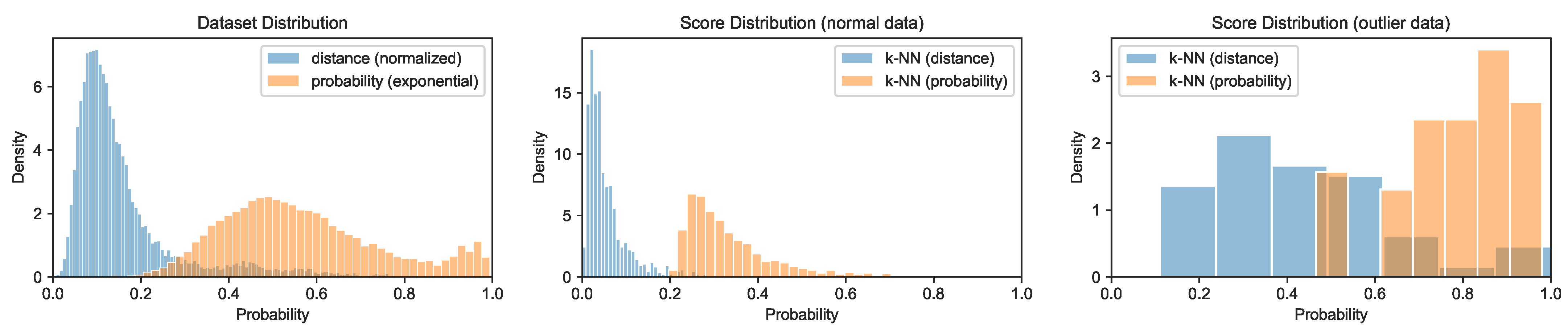
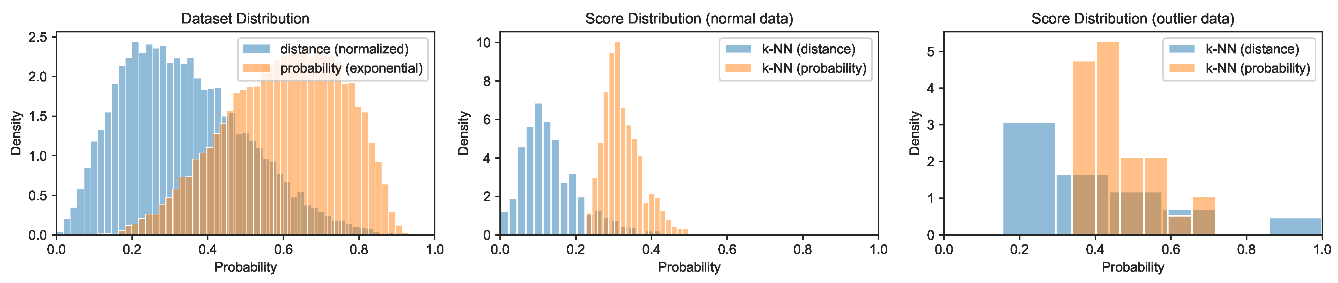
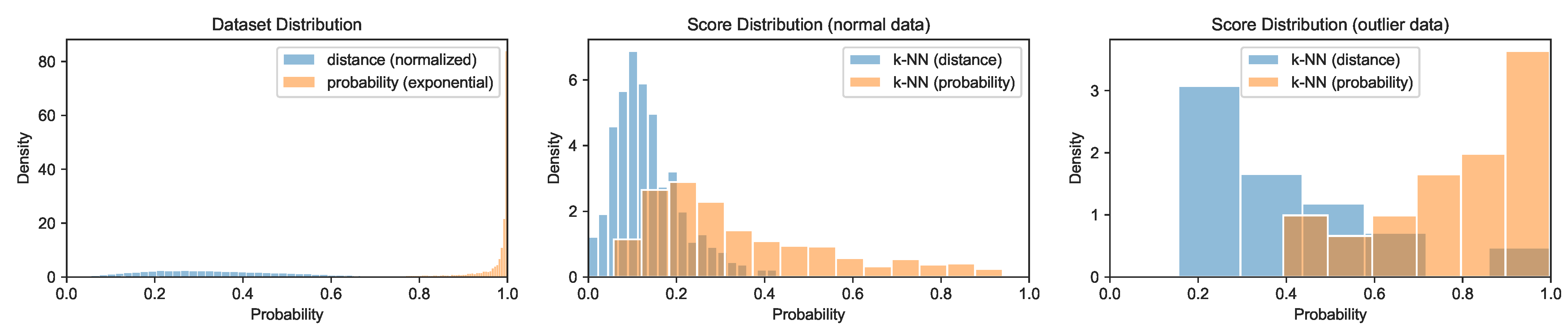
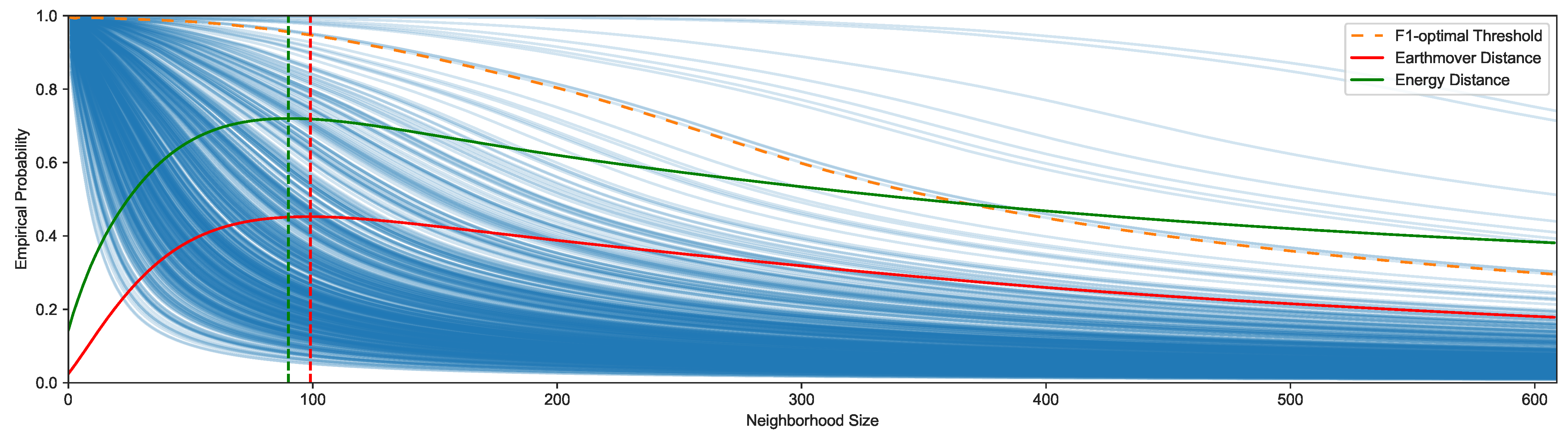
From an interpretability perspective, there are datasets where using the entire distance matrix as a normalization set results in useful probabilistic estimates, for example, the Crop dataset shown in Figure 5. However, using the entire distance matrix for normalization often leads to low probabilistic estimates for normal and outlier data points. The reason is that the resulting weighted neighbor distance is consistently low compared to all other distances in the dataset, even for outliers. In this case, a different normalization set has to be extracted from the distance matrix; for example, the m-neighborhood consisting of the distances to the m-closest reference points. It is possible to analyze multiple normalization sets for the outlier score predictions to provide more context for interpretation, a process we term probabilistic neighborhood analysis. For example, predictions can be interpreted using neighborhood probabilities from $m\in [1,2,\dots ,1024]$, resulting in different score distributions and different cut-off thresholds. The cut-off decision relies on the characteristics of the score distribution and is determined using statistical measures such as the median absolute deviation, domain knowledge or, when labels are available, performance metrics for binary classification [101,102]. To give an example for the TwoLeadECG dataset, in Figure 6 and Figure 7, we compare the initial probabilistic estimates using the entire distance matrix to a smaller, local normalization set identified using a probabilistic neighborhood analysis as shown in Figure 8. Using statistical measures of contrast, we derive a contrast-optimal neighborhood size of $m=90$ or $m=99$ depending on the statistical distance used, with a cut-off threshold of approximately 95%, as shown in Figure 8. The probabilistic neighborhood analysis clearly demonstrates the increased contrast using a smaller normalization set and additionally depicts the optimal cut-off threshold for different neighborhood sizes. Nonetheless, we note that an optimal cut-off threshold is difficult to determine in an unsupervised setting. To identify an optimal cut-off threshold, it is necessary to evaluate it against a performance metric such as the F1-score requiring normal and outlier labeled data, which are often unavailable. Using a probabilistic neighborhood analysis simplifies the identification of a suitable cut-off value, even when labels are unavailable. Thus, in addition to the improved interpretability, choosing an appropriate normalization set allows for a flexible definition of a cut-off threshold to transform outlier scores into class labels. Furthermore, it is possible to increase the contrast between normal and outlier data points using the right normalization set. Using statistical distances as a measure of contrast between normal and outlier scores, we can identify an optimal normalization set as shown in Figure 8.

For image-based datasets, we extend the PatchCore methodology [34] to ProbabilisticPatchCore, by transforming the distance-based patches using our probabilistic normalization approach with an empirical distribution. We evaluate the model on the datasets provided by MVTecAD, as shown in

Table 3. MVTecAD [85] image datasets for the evaluation of ProbabilisticPatchCore.

Dataset	Train (Normal)	Test (Normal)	Test (Outlier)	Masks	Groups	Shape
Carpet	280	28	89	97	5	$1024\times 1024$
Grid	264	21	57	170	5	$1024\times 1024$
Leather	245	32	92	99	5	$1024\times 1024$
Tile	230	33	84	86	5	$840\times 840$
Wood	247	19	60	168	5	$1024\times 1024$
Bottle	209	20	63	68	3	$900\times 900$
Cable	224	58	92	151	8	$1024\times 1024$
Capsule	219	23	109	114	5	$1000\times 1000$
Hazelnut	391	40	70	136	4	$1024\times 1024$
Metal Nut	220	22	93	132	4	$700\times 700$
Pill	267	26	141	245	7	$800\times 800$
Screw	320	41	119	135	5	$1024\times 1024$
Toothbrush	60	12	30	66	1	$1024\times 1024$
Transistor	213	60	40	44	4	$1024\times 1024$
Zipper	240	32	119	177	7	$1024\times 1024$

. A major difference between tabular k-nearest neighbors outlier detection and image outlier detection is that the image models may result in pixel-wise and image-wise outlier scores. In the pixel-wise case, each pixel of an observation is scored and in the image-wise case a single score is obtained for the entire image.

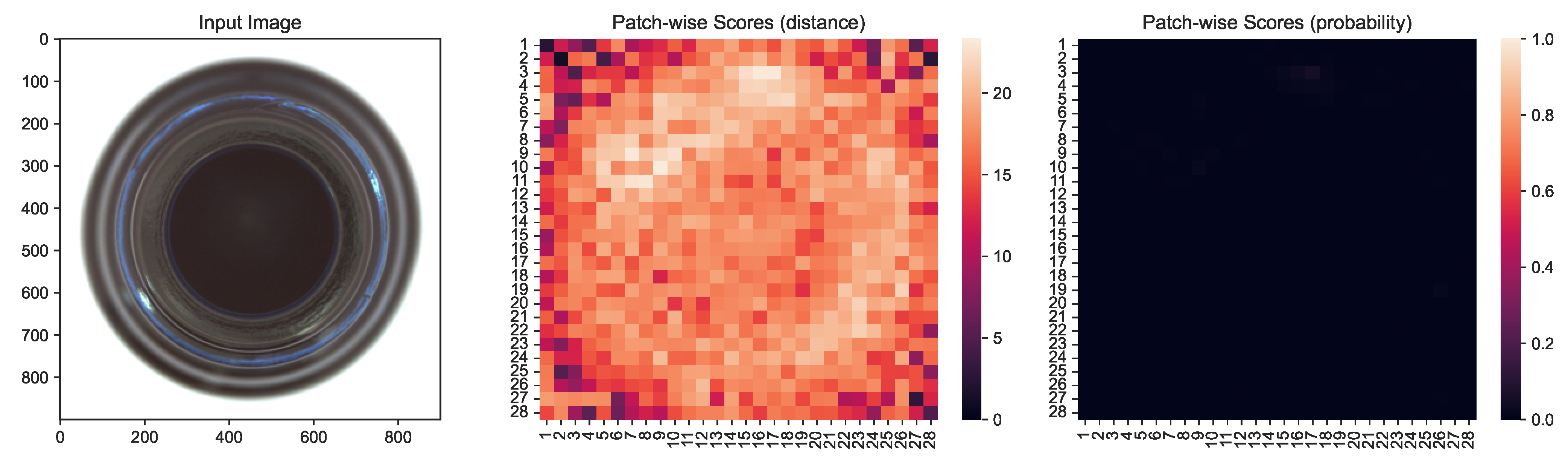
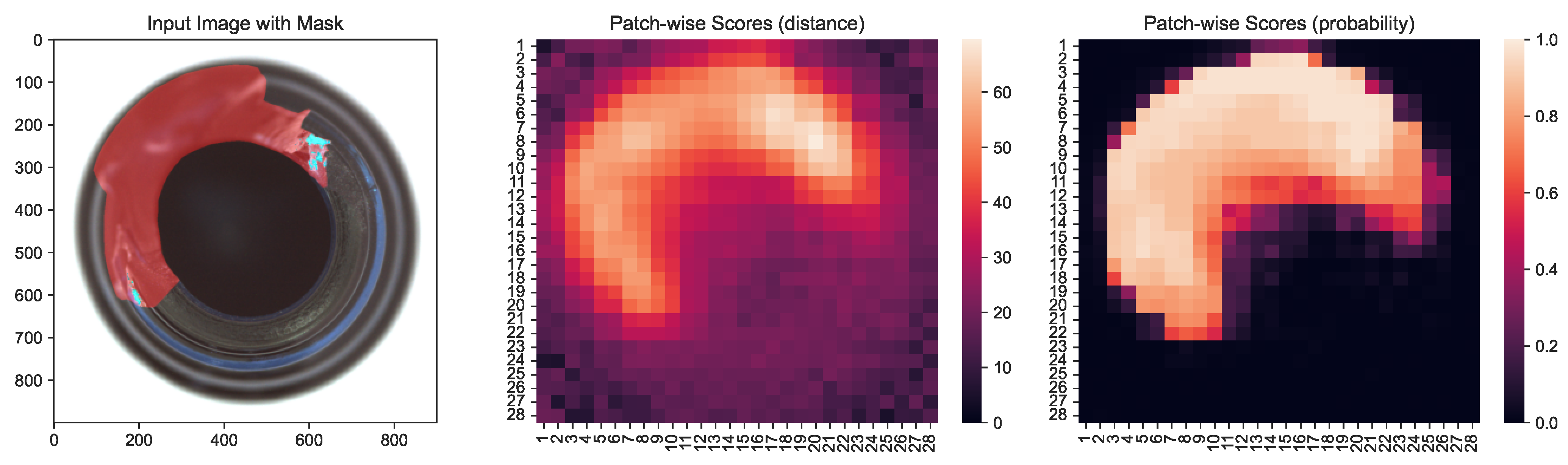
The PatchCore model is similar to $k^{\mathrm{th}}\mathrm{NN}$, but uses a core-set sampled memory bank of patch-wise feature vectors that are generated using a pre-trained neural network. For PatchCore, the pixel-wise scores are determined through interpolation of the patch-wise scores; thus, it is not necessary to estimate a distance distribution per pixel, but one distribution per patch. Like the authors, we used the second and third layer of a WideResNet50 trained on ImageNet [103] to determine $28\times 28$ patches. Additionally, we used a single neighbor corresponding to the patch-wise $k^{\mathrm{th}}\mathrm{NN}$ approach with a core-set sampling ratio of 10%. To transform the pixel-wise scores into probabilistic estimates, we estimated patch-wise distributions and transformed the scores for each patch to probabilistic estimates accordingly. To determine an appropriate normalization set for each image-based dataset, we identified the optimal set in an m-neighborhood of $m\in [1,2,\dots ,1024]$ with the largest contrast. We established the contrast between normal and outlier samples as the Earthmover distance between the image-level score distributions. We demonstrate that there are no significant ranking or detection differences between PatchCore and ProbabilisticPatchCore in

Table 4. Mean image-level and pixel-level ROC AUC scores and image-level F1 scores over all image datasets in MVTecAD to compare PatchCore and ProbabilisticPatchCore regarding ranking stability and detection performance.

	F1 (Image)	ROC AUC (Image)	ROC AUC (Pixel)
PatchCore	0.978 ± 0.012	0.987 ± 0.017	0.976 ± 0.017
ProbabilisticPatchCore	0.971 ± 0.021	0.982 ± 0.023	0.976 ± 0.016

and provide a more detailed analysis of the results online (https://davnn.github.io/probabilistic-distance/, accessed on 1 June 2023). In Figure 9, we highlight the challenge of interpretability based on a normal data sample; without additional context, it is not clear how to interpret the resulting distance-based scores. In addition to the improved interpretability, we find that the probabilistic normalization greatly increases the contrast between normal and outlier data points in the image detection tasks, as visible in Figure 10.

6. Conclusions

We show that it is possible to transform distance-based outlier scores into interpretable probabilistic estimates with increased contrast. Determining the “real” outliers from outlier scores is one of the main challenges in real-world outlier detection scenarios such as network intrusion detection, fraud detection, medical diagnostics, proficiency testing, or industrial quality control. Our probabilistic normalization markedly simplifies the process to convert outlier scores into meaningful decisions by providing an interpretable result with a clear separation between normal and outlier data points. To demonstrate the viability of our approach, we derive and test a generalized, weighted k-nearest neighbors outlier detection model ($\mathrm{kNNW}$) on several tabular datasets and a probabilistic patch-wise model (ProbabilisticPatchCore) on image datasets. We show that the resulting probabilistic scores increase the contrast between normal and outlier data points and can easily be added to existing distance-based outlier detection methods. In comparison to previous score normalization techniques, which use solely the information contained in the outlier scores to derive a normalization, we make use of the distances to other data points as an additional source of information for normalization. Another interesting aspect of our analysis is showing that the probabilistic transformation increases the contrast between normal and outlier points, which should be further explored in more detail. The increased contrast simplifies downstream tasks since it becomes easier to differentiate normal from outlier data points, a fundamental motivation for our transformation and an essential characteristic of outliers, as pointed out by Hawkins [3]: “a sample containing outliers would show up such characteristics as large gaps between ‘outlying’ and ‘inlying’ observations and the deviation between outliers and the group of inliers, as measured on some suitably standardized scale”. We hypothesize that there might be an optimal normalization set that maximally increases the contrast between normal and outlier points and future research is necessary to define measures of contrast and methods to identify an optimal normalization set for a given contrast measure. Because distance-based outlier detection techniques rely on distance computations for nearest-neighbor search, our approach can be applied to a wide range of detection techniques. In our experiments, we used the common Euclidean distance metric, but other, possibly non-metric, distance measures are also used for outlier detection, and should also be investigated using our probabilistic score transformation. We investigated only the most apparent normalization sets, but there may be various other useful normalization sets hidden in the distances between points. Another limitation of our examination is the usage of real-world datasets, which limits the theoretical analysis of our approach, such as the normalization behavior under specific dataset distributions. Our proposed normalization approach should be investigated more thoroughly in a theoretical setting to identify the limits of our approach and potentially prove some of the properties observed in our evaluation. Another limitation of our investigation is the use of non-robust estimation techniques, and the influence of estimator robustness should be explored in future research. Our proposed generalization of weighted nearest-neighbor outlier detection should be analyzed in more detail to thoroughly compare weighting strategies and weighting hyperparameters. A large body of research investigates sampling and subspacing techniques for distance-based outlier detection and future researchers should evaluate the usefulness of probabilistic intepretations for such models. Another important area of outlier detection research is how to combine different detection models into ensembles that improve upon the individual models, which typically necessitate score normalization and, therefore, could benefit from probabilistic normalization. We further highlight the importance of a distinction between the open-world and closed-world settings for distance-based outlier detection and propose such a distinction for future distance-based methods.

References

- Barnett, V.; Lewis, T. Outliers in Statistical Data; John Wiley & Sons, Inc.: Hoboken, NJ, USA, 1978. [Google Scholar]
- Ruff, L.; Kauffmann, J.R.; Vandermeulen, R.A.; Montavon, G.; Samek, W.; Kloft, M.; Dietterich, T.G.; Müller, K.R. A Unifying Review of Deep and Shallow Anomaly Detection. Proc. IEEE 2021, 109, 756–795. [Google Scholar] [CrossRef]
- Hawkins, D.M. Identification of Outliers; Springer: Dordrecht, The Netherlands, 1980. [Google Scholar] [CrossRef]
- Markou, M.; Singh, S. Novelty Detection: A Review—Part 1: Statistical Approaches. Signal Process. 2003, 83, 2481–2497. [Google Scholar] [CrossRef]
- Markou, M.; Singh, S. Novelty Detection: A Review—Part 2. Signal Process. 2003, 83, 2499–2521. [Google Scholar] [CrossRef]
- Hodge, V.; Austin, J. A Survey of Outlier Detection Methodologies. Artif. Intell. Rev. 2004, 22, 85–126. [Google Scholar] [CrossRef] [Green Version]
- Chandola, V.; Banerjee, A.; Kumar, V. Anomaly Detection. ACM Comput. Surv. 2009, 41, 1–58. [Google Scholar] [CrossRef]
- Pimentel, M.A.; Clifton, D.A.; Clifton, L.; Tarassenko, L. A Review of Novelty Detection. Signal Process. 2014, 99, 215–249. [Google Scholar] [CrossRef]
- Knorr, E.M.; Ng, R.T. A Unified Approach for Mining Outliers. In Proceedings of the CASCON ’97: Proceedings of the 1997 Conference of the Centre for Advanced Studies on Collaborative Research, Toronto, ON, USA, 10–13 November 1997; p. 11. [Google Scholar] [CrossRef]
- Knorr, E.M.; Ng, R.T. Algorithms for Mining Distance-Based Outliers in Large Datasets. In Proceedings of the 24rd International Conference on Very Large Data Bases, New York, NY, USA, 24–27 August 1998; VLDB ’98. Morgan Kaufmann Publishers Inc.: San Francisco, CA, USA, 1998; pp. 392–403. [Google Scholar]
- Knorr, E.M.; Ng, R.T.; Tucakov, V. Distance-Based Outliers: Algorithms and Applications. Vldb J. Int. J. Very Large Data Bases 2000, 8, 237–253. [Google Scholar] [CrossRef]
- Ramaswamy, S.; Rastogi, R.; Shim, K. Efficient Algorithms for Mining Outliers from Large Data Sets. SIGMOD Rec. 2000, 29, 427–438. [Google Scholar] [CrossRef]
- Angiulli, F.; Pizzuti, C. Fast Outlier Detection in High Dimensional Spaces. In Principles of Data Mining and Knowledge Discovery; Goos, G., Hartmanis, J., van Leeuwen, J., Carbonell, J.G., Siekmann, J., Elomaa, T., Mannila, H., Toivonen, H., Eds.; Lecture Notes in Computer Science; Springer: Berlin/Heidelberg, Germany, 2002; pp. 15–27. [Google Scholar] [CrossRef] [Green Version]
- Geler, Z.; Kurbalija, V.; Radovanović, M.; Ivanović, M. Comparison of Different Weighting Schemes for the kNN Classifier on Time-Series Data. Knowl. Inf. Syst. 2016, 48, 331–378. [Google Scholar] [CrossRef]
- Dudani, S.A. The Distance-Weighted k-Nearest-Neighbor Rule. IEEE Trans. Syst. Man Cybern. 1976, SMC-6, 325–327. [Google Scholar] [CrossRef]
- Zavrel, J. An Empirical Re-Examination of Weighted Voting for k-NN. In Proceedings of the BENELEARN-97 7th Belgian-Dutch Conference on Machine Learning, Tilburg, The Netherlands, 21 October 1997; Daelemans, W., Flach, P., van den Bosch, A., Eds.; Tilburg University: Tilburg, The Netherlands, 1997; pp. 139–145. [Google Scholar]
- Macleod, J.E.S.; Luk, A.; Titterington, D.M. A Re-Examination of the Distance-Weighted k-Nearest Neighbor Classification Rule. IEEE Trans. Syst. Man Cybern. 1987, 17, 689–696. [Google Scholar] [CrossRef]
- Wu, M.; Jermaine, C. Outlier Detection by Sampling with Accuracy Guarantees. In Proceedings of the 12th ACM SIGKDD International Conference on Knowledge Discovery and Data Mining, Philadelphia, PA, USA, 20–23 August 2006; pp. 767–772. [Google Scholar] [CrossRef]
- Sugiyama, M.; Borgwardt, K. Rapid Distance-Based Outlier Detection via Sampling. In Proceedings of the Advances in Neural Information Processing Systems; Curran Associates, Inc.: Red Hook, NY, USA, 2013; Volume 26. [Google Scholar]
- Pang, G.; Ting, K.M.; Albrecht, D. LeSiNN: Detecting Anomalies by Identifying Least Similar Nearest Neighbours. In Proceedings of the 2015 IEEE International Conference on Data Mining Workshop (ICDMW), Atlantic City, NJ, USA, 14–17 November 2015; pp. 623–630. [Google Scholar] [CrossRef]
- Zimek, A.; Gaudet, M.; Campello, R.J.; Sander, J. Subsampling for Efficient and Effective Unsupervised Outlier Detection Ensembles. In Proceedings of the 19th ACM SIGKDD International Conference on Knowledge Discovery and Data Mining, Chicago, IL, USA, 11–14 August 2013; KDD ’13. Association for Computing Machinery: New York, NY, USA, 2013; pp. 428–436. [Google Scholar] [CrossRef] [Green Version]
- Aggarwal, C.C.; Sathe, S. Theoretical Foundations and Algorithms for Outlier Ensembles. ACM Sigkdd Explor. Newsl. 2015, 17, 24–47. [Google Scholar] [CrossRef]
- Muhr, D.; Affenzeller, M. Little Data Is Often Enough for Distance-Based Outlier Detection. Procedia Comput. Sci. 2022, 200, 984–992. [Google Scholar] [CrossRef]
- Aggarwal, C.; Yu, P. Outlier Detection for High Dimensional Data. ACM SIGMOD Rec. 2002, 30. [Google Scholar] [CrossRef]
- Kriegel, H.P.; Kröger, P.; Schubert, E.; Zimek, A. Outlier Detection in Axis-Parallel Subspaces of High Dimensional Data. In Advances in Knowledge Discovery and Data Mining; Theeramunkong, T., Kijsirikul, B., Cercone, N., Ho, T.B., Eds.; Lecture Notes in Computer Science; Springer: Berlin/Heidelberg, Germany, 2009; pp. 831–838. [Google Scholar] [CrossRef] [Green Version]
- Agrawal, A. Local Subspace Based Outlier Detection. In Contemporary Computing; Ranka, S., Aluru, S., Buyya, R., Chung, Y.C., Dua, S., Grama, A., Gupta, S.K.S., Kumar, R., Phoha, V.V., Eds.; Communications in Computer and Information Science; Springer: Berlin/Heidelberg, Germany, 2009; pp. 149–157. [Google Scholar] [CrossRef]
- Zhang, L.; Lin, J.; Karim, R. An Angle-Based Subspace Anomaly Detection Approach to High-Dimensional Data: With an Application to Industrial Fault Detection. Reliab. Eng. Syst. Saf. 2015, 142, 482–497. [Google Scholar] [CrossRef] [Green Version]
- Trittenbach, H.; Böhm, K. Dimension-Based Subspace Search for Outlier Detection. Int. J. Data Sci. Anal. 2019, 7, 87–101. [Google Scholar] [CrossRef]
- Keller, F.; Muller, E.; Bohm, K. HiCS: High Contrast Subspaces for Density-Based Outlier Ranking. In Proceedings of the 2012 IEEE 28th International Conference on Data Engineering, Arlington, VA, USA, 1–5 April 2012; pp. 1037–1048. [Google Scholar] [CrossRef] [Green Version]
- Cabero, I.; Epifanio, I.; Piérola, A.; Ballester, A. Archetype Analysis: A New Subspace Outlier Detection Approach. Knowl.-Based Syst. 2021, 217, 106830. [Google Scholar] [CrossRef]
- Dang, T.T.; Ngan, H.Y.; Liu, W. Distance-Based k-Nearest Neighbors Outlier Detection Method in Large-Scale Traffic Data. In Proceedings of the 2015 IEEE International Conference on Digital Signal Processing (DSP), Singapore, 21–24 July 2015; pp. 507–510. [Google Scholar] [CrossRef]
- Bergman, L.; Cohen, N.; Hoshen, Y. Deep Nearest Neighbor Anomaly Detection. arXiv 2020, arXiv:2002.10445. [Google Scholar]
- Cohen, N.; Hoshen, Y. Sub-Image Anomaly Detection with Deep Pyramid Correspondences. arXiv 2021, arXiv:2005.02357. [Google Scholar]
- Roth, K.; Pemula, L.; Zepeda, J.; Scholkopf, B.; Brox, T.; Gehler, P. Towards Total Recall in Industrial Anomaly Detection. In Proceedings of the 2022 IEEE/CVF Conference on Computer Vision and Pattern Recognition (CVPR), New Orleans, LA, USA, 19–24 June 2022; pp. 14298–14308. [Google Scholar] [CrossRef]
- Hautamaki, V.; Karkkainen, I.; Franti, P. Outlier Detection Using K-Nearest Neighbour Graph. In Proceedings of the 17th International Conference on Pattern Recognition, Cambridge, UK, 26 August 2004; Volume 3, pp. 430–433. [Google Scholar] [CrossRef] [Green Version]
- Radovanović, M.; Nanopoulos, A.; Ivanović, M. Reverse Nearest Neighbors in Unsupervised Distance-Based Outlier Detection. IEEE Trans. Knowl. Data Eng. 2015, 27, 1369–1382. [Google Scholar] [CrossRef]
- Zhu, Q.; Feng, J.; Huang, J. Natural Neighbor: A Self-Adaptive Neighborhood Method without Parameter K. Pattern Recognit. Lett. 2016, 80, 30–36. [Google Scholar] [CrossRef]
- Wahid, A.; Annavarapu, C.S.R. NaNOD: A Natural Neighbour-Based Outlier Detection Algorithm. Neural Comput. Appl. 2021, 33, 2107–2123. [Google Scholar] [CrossRef]
- Tang, B.; He, H. ENN: Extended Nearest Neighbor Method for Pattern Recognition [Research Frontier]. IEEE Comput. Intell. Mag. 2015, 10, 52–60. [Google Scholar] [CrossRef]
- Tang, B.; He, H. A Local Density-Based Approach for Outlier Detection. Neurocomputing 2017, 241, 171–180. [Google Scholar] [CrossRef] [Green Version]
- Breunig, M.M.; Kriegel, H.P.; Ng, R.T.; Sander, J. LOF: Identifying Density-Based Local Outliers. In Proceedings of the 2000 ACM SIGMOD International Conference on Management of Data: 2000, Dallas, TX, USA, 15–18 May 2000; Dunham, M., Naughton, J.F., Chen, W., Koudas, N., Eds.; Association for Computing Machinery: New York, NY, USA, 2000; pp. 93–104. [Google Scholar] [CrossRef]
- Schubert, E.; Zimek, A.; Kriegel, H.P. Local Outlier Detection Reconsidered: A Generalized View on Locality with Applications to Spatial, Video, and Network Outlier Detection. Data Min. Knowl. Discov. 2014, 28, 190–237. [Google Scholar] [CrossRef]
- Schubert, E.; Zimek, A.; Kriegel, H.P. Generalized Outlier Detection with Flexible Kernel Density Estimates. In Proceedings of the 2014 SIAM International Conference on Data Mining, Philadelphia, PA, USA, 24–26 April 2014; Zaki, M., Obradovic, Z., Tan, P.N., Banerjee, A., Kamath, C., Parthasarathy, S., Eds.; Society for Industrial and Applied Mathematics: Philadelphia, PA, USA, 2014; pp. 542–550. [Google Scholar] [CrossRef] [Green Version]
- Zhang, K.; Hutter, M.; Jin, H. A New Local Distance-Based Outlier Detection Approach for Scattered Real-World Data. In Advances in Knowledge Discovery and Data Mining, Proceedings of the 13th Pacific-Asia Conference, PAKDD 2009, Bangkok, Thailand, 27–30 April 2009; Theeramunkong, T., Kijsirikul, B., Cercone, N., Ho, T.B., Eds.; Springer: Berlin/Heidelberg, Germany, 2009; Lecture Notes in Computer Science, 0302-9743; Volume 5476, pp. 813–822. [Google Scholar]
- Jin, W.; Tung, A.K.H.; Han, J.; Wang, W. Ranking Outliers Using Symmetric Neighborhood Relationship. In Proceedings of the Advances in Knowledge Discovery and Data Mining; Ng, W.K., Kitsuregawa, M., Li, J., Chang, K., Eds.; Springer: Berlin/Heidelberg, Germany, 2006; Lecture Notes in Computer Science; pp. 577–593. [Google Scholar] [CrossRef] [Green Version]
- Kriegel, H.P.; Kröger, P.; Schubert, E.; Zimek, A. LoOP: Local Outlier Probabilities. In Proceedings of the 18th ACM Conference on Information and Knowledge Management, Hong Kong, China, 2–6 November 2009; Cheung, D.W.L., Song, I.Y., Chu, W.W., Hu, X., Lin, J.J., Eds.; Association for Computing Machinery: New York, NY, USA, 2009; pp. 1649–1652. [Google Scholar] [CrossRef]
- Alghushairy, O.; Alsini, R.; Soule, T.; Ma, X. A Review of Local Outlier Factor Algorithms for Outlier Detection in Big Data Streams. Big Data Cogn. Comput. 2021, 5, 1. [Google Scholar] [CrossRef]
- Goodge, A.; Hooi, B.; Ng, S.K.; Ng, W.S. LUNAR: Unifying Local Outlier Detection Methods via Graph Neural Networks. In Proceedings of the AAAI Conference on Artificial Intelligence, Virtual Event, 22 February–1 March 2022. [Google Scholar]
- Zhao, Y.; Nasrullah, Z.; Li, Z. PyOD: A Python Toolbox for Scalable Outlier Detection. J. Mach. Learn. Res. 2019, 20, 1–7. [Google Scholar]
- Muhr, D.; Affenzeller, M.; Blaom, A.D. OutlierDetection.Jl: A Modular Outlier Detection Ecosystem for the Julia Programming Language. arXiv 2022, arXiv:2211.04550. [Google Scholar]
- Kriegel, H.P.; Kröger, P.; Schubert, E.; Zimek, A. Outlier Detection in Arbitrarily Oriented Subspaces. In Proceedings of the 2012 IEEE 12th International Conference on Data Mining, Brussels, Belgium, 10–13 December 2012; pp. 379–388. [Google Scholar] [CrossRef]
- Janssens, J.; Huszár, F.; Postma, E. Stochastic Outlier Selection; Technical Report TiCC TR 2012–001; Tilburg University: Tilburg, The Netherlands, 2012. [Google Scholar]
- van Stein, B.; van Leeuwen, M.; Bäck, T. Local Subspace-Based Outlier Detection Using Global Neighbourhoods. In Proceedings of the 2016 IEEE International Conference on Big Data, Washington, WA, USA, 5–8 December 2016; pp. 1136–1142. [Google Scholar] [CrossRef] [Green Version]
- Latecki, L.J.; Lazarevic, A.; Pokrajac, D. Outlier Detection with Kernel Density Functions. In Proceedings of the Machine Learning and Data Mining in Pattern Recognition, Leipzig, Germany, 18–20 July 2007; Perner, P., Ed.; Lecture Notes in Computer Science. Springer: Berlin/Heidelberg, Germany, 2007; pp. 61–75. [Google Scholar] [CrossRef] [Green Version]
- Gao, J.; Tan, P.N. Converting Output Scores from Outlier Detection Algorithms into Probability Estimates. In Proceedings of the Sixth International Conference on Data Mining (ICDM’06), Hong Kong, China, 18–22 December 2006; pp. 212–221. [Google Scholar] [CrossRef]
- Kriegel, H.P.; Kroger, P.; Schubert, E.; Zimek, A. Interpreting and Unifying Outlier Scores. In Proceedings of the 2011 SIAM International Conference on Data Mining, Mesa, AZ, USA, 28–30 April 2011; Liu, B., Liu, H., Clifton, C., Washio, T., Kamath, C., Eds.; Society for Industrial and Applied Mathematics: Philadelphia, PA, USA, 2011; pp. 13–24. [Google Scholar] [CrossRef] [Green Version]
- Bouguessa, M. Modeling Outlier Score Distributions. In Proceedings of the Advanced Data Mining and Applications; Lecture Notes in Computer Science. Zhou, S., Zhang, S., Karypis, G., Eds.; Springer: Berlin/Heidelberg, Germany, 2012; pp. 713–725. [Google Scholar] [CrossRef]
- Schubert, E.; Wojdanowski, R.; Zimek, A.; Kriegel, H.P. On Evaluation of Outlier Rankings and Outlier Scores. In Proceedings of the 2012 SIAM International Conference on Data Mining, Anaheim, CA, USA, 26–28 April 2012; Ghosh, J., Liu, H., Davidson, I., Domeniconi, C., Kamath, C., Eds.; Society for Industrial and Applied Mathematics: Philadelphia, PA, USA, 2012; pp. 1047–1058. [Google Scholar] [CrossRef] [Green Version]
- Li, X.; Xiong, H.; Li, X.; Wu, X.; Zhang, X.; Liu, J.; Bian, J.; Dou, D. Interpretable Deep Learning: Interpretation, Interpretability, Trustworthiness, and Beyond. Knowl. Inf. Syst. 2022, 64, 3197–3234. [Google Scholar] [CrossRef]
- Zimek, A.; Filzmoser, P. There and Back Again: Outlier Detection between Statistical Reasoning and Data Mining Algorithms. WIREs Data Min. Knowl. Discov. 2018, 8, e1280. [Google Scholar] [CrossRef] [Green Version]
- Micenková, B.; Ng, R.T.; Dang, X.H.; Assent, I. Explaining Outliers by Subspace Separability. In Proceedings of the 2013 IEEE International Conference on Data Mining, Dallas, TX, USA, 7–10 December 2013; pp. 518–527. [Google Scholar] [CrossRef]
- Vinh, N.X.; Chan, J.; Romano, S.; Bailey, J.; Leckie, C.; Ramamohanarao, K.; Pei, J. Discovering Outlying Aspects in Large Datasets. Data Min. Knowl. Discov. 2016, 30, 1520–1555. [Google Scholar] [CrossRef]
- Macha, M.; Akoglu, L. Explaining Anomalies in Groups with Characterizing Subspace Rules. Data Min. Knowl. Discov. 2018, 32, 1444–1480. [Google Scholar] [CrossRef] [Green Version]
- Angiulli, F.; Fassetti, F.; Palopoli, L. Discovering Characterizations of the Behavior of Anomalous Subpopulations. IEEE Trans. Knowl. Data Eng. 2013, 25, 1280–1292. [Google Scholar] [CrossRef]
- Samek, W.; Montavon, G.; Vedaldi, A.; Hansen, L.K.; Müller, K.R. (Eds.) Explainable AI: Interpreting, Explaining and Visualizing Deep Learning; Lecture Notes in Computer Science; Springer International Publishing: Cham, Switzerland, 2019; Volume 11700. [Google Scholar] [CrossRef]
- Lapuschkin, S.; Wäldchen, S.; Binder, A.; Montavon, G.; Samek, W.; Müller, K.R. Unmasking Clever Hans Predictors and Assessing What Machines Really Learn. Nat. Commun. 2019, 10, 1096. [Google Scholar] [CrossRef] [Green Version]
- Kauffmann, J.; Ruff, L.; Montavon, G.; Müller, K.R. The Clever Hans Effect in Anomaly Detection. arXiv 2020, arXiv:2006.10609. [Google Scholar]
- Lee, J.D.; See, K.A. Trust in Automation: Designing for Appropriate Reliance. Hum. Factors 2004, 46, 50–80. [Google Scholar] [CrossRef] [Green Version]
- Jiang, H.; Kim, B.; Guan, M.; Gupta, M. To Trust or Not to Trust a Classifier. In Proceedings of the Advances in Neural Information Processing Systems; Curran Associates, Inc.: Red Hook, NY, USA, 2018; Volume 31. [Google Scholar]
- Ovadia, Y.; Fertig, E.; Ren, J.; Nado, Z.; Sculley, D.; Nowozin, S.; Dillon, J.; Lakshminarayanan, B.; Snoek, J. Can You Trust Your Model’s Uncertainty? Evaluating Predictive Uncertainty under Dataset Shift. In Proceedings of the Advances in Neural Information Processing Systems; Curran Associates, Inc.: Red Hook, NY, USA, 2019; Volume 32. [Google Scholar]
- Perini, L.; Vercruyssen, V.; Davis, J. Quantifying the Confidence of Anomaly Detectors in Their Example-Wise Predictions. In Proceedings of the Machine Learning and Knowledge Discovery in Databases; Lecture Notes in Computer Science; Hutter, F., Kersting, K., Lijffijt, J., Valera, I., Eds.; Springer: Cham, Switzerland, 2021; pp. 227–243. [Google Scholar] [CrossRef]
- Muhr, D.; Affenzeller, M. Hybrid (CPU/GPU) Exact Nearest Neighbors Search in High-Dimensional Spaces. In Proceedings of the Artificial Intelligence Applications and Innovations; IFIP Advances in Information and Communication Technology; Maglogiannis, I., Iliadis, L., Macintyre, J., Cortez, P., Eds.; Springer: Cham, Switzerland, 2022; pp. 112–123. [Google Scholar] [CrossRef]
- Kirner, E.; Schubert, E.; Zimek, A. Good and Bad Neighborhood Approximations for Outlier Detection Ensembles. Lect. Notes Comput. Sci. 2017, 10609, 173–187. [Google Scholar] [CrossRef]
- Burghouts, G.; Smeulders, A.; Geusebroek, J.M. The Distribution Family of Similarity Distances. In Proceedings of the Advances in Neural Information Processing Systems; Curran Associates, Inc.: Red Hook, NY, USA, 2007; Volume 20. [Google Scholar]
- Schnitzer, D.; Flexer, A.; Schedl, M.; Widmer, G. Local and Global Scaling Reduce Hubs in Space. J. Mach. Learn. Res. 2012, 13, 2871–2902. [Google Scholar]
- Houle, M.E. Dimensionality, Discriminability, Density and Distance Distributions. In Proceedings of the 2013 IEEE 13th International Conference on Data Mining Workshops, Dallas, TX, USA, 7–10 December 2013; pp. 468–473. [Google Scholar] [CrossRef]
- Lellouche, S.; Souris, M. Distribution of Distances between Elements in a Compact Set. Stats 2020, 3, 1–15. [Google Scholar] [CrossRef] [Green Version]
- Pekalska, E.; Duin, R. Classifiers for Dissimilarity-Based Pattern Recognition. In Proceedings of the 15th International Conference on Pattern Recognition, ICPR-2000, Barcelona, Spain, 3–8 September 2000; Volume 2, pp. 12–16. [Google Scholar] [CrossRef]
- Hubert, M.; Debruyne, M. Breakdown Value. Wires Comput. Stat. 2009, 1, 296–302. [Google Scholar] [CrossRef]
- Rousseeuw, P.J.; Hubert, M. Robust Statistics for Outlier Detection. Wires Data Min. Knowl. Discov. 2011, 1, 73–79. [Google Scholar] [CrossRef]
- Kim, J.; Scott, C.D. Robust Kernel Density Estimation. J. Mach. Learn. Res. 2012, 13, 2529–2565. [Google Scholar]
- Campos, G.O.; Zimek, A.; Sander, J.; Campello, R.J.G.B.; Micenková, B.; Schubert, E.; Assent, I.; Houle, M.E. On the Evaluation of Unsupervised Outlier Detection: Measures, Datasets, and an Empirical Study. Data Min. Knowl. Discov. 2016, 30, 891–927. [Google Scholar] [CrossRef]
- Muhr, D.; Affenzeller, M. Outlier/Anomaly Detection of Univariate Time Series: A Dataset Collection and Benchmark. In Proceedings of the Big Data Analytics and Knowledge Discovery; Wrembel, R., Gamper, J., Kotsis, G., Tjoa, A.M., Khalil, I., Eds.; Lecture Notes in Computer Science; Springer: Cham, Switzerland, 2022; pp. 163–169. [Google Scholar] [CrossRef]
- Bergmann, P.; Fauser, M.; Sattlegger, D.; Steger, C. MVTec AD—A Comprehensive Real-World Dataset for Unsupervised Anomaly Detection. In Proceedings of the 2019 IEEE/CVF Conference on Computer Vision and Pattern Recognition (CVPR), Long Beach, CA, USA, 16–20 June 2019; pp. 9584–9592. [Google Scholar] [CrossRef]
- Bergmann, P.; Batzner, K.; Fauser, M.; Sattlegger, D.; Steger, C. The MVTec Anomaly Detection Dataset: A Comprehensive Real-World Dataset for Unsupervised Anomaly Detection. Int. J. Comput. Vis. 2021, 129, 1038–1059. [Google Scholar] [CrossRef]
- Dua, D.; Graff, C. The UCI Machine Learning Repository. 2017. Available online: http://archive.ics.uci.edu/ml (accessed on 1 June 2023).
- Goldberger, A.L.; Amaral, L.A.N.; Glass, L.; Hausdorff, J.M.; Ivanov, P.C.; Mark, R.G.; Mietus, J.E.; Moody, G.B.; Peng, C.K.; Stanley, H.E. PhysioBank, PhysioToolkit, and PhysioNet: Components of a New Research Resource for Complex Physiologic Signals. Circulation 2000, 101, e215. [Google Scholar] [CrossRef] [Green Version]
- Tan, C.W.; Webb, G.I.; Petitjean, F. Indexing and Classifying Gigabytes of Time Series under Time Warping. In Proceedings of the 2017 SIAM International Conference on Data Mining (SDM), Houston, TX, USA, 27–29 April 2017; Society for Industrial and Applied Mathematics: Philadelphia, PA, USA, 2017; pp. 282–290. [Google Scholar] [CrossRef] [Green Version]
- Dau, H.A.; Bagnall, A.; Kamgar, K.; Yeh, C.C.M.; Zhu, Y.; Gharghabi, S.; Ratanamahatana, C.A.; Keogh, E. The UCR Time Series Archive. IEEE/CAA J. Autom. Sin. 2019, 6, 1293–1305. [Google Scholar] [CrossRef]
- Murray, D.; Liao, J.; Stankovic, L.; Stankovic, V.; Hauxwell-Baldwin, R.; Wilson, C.; Coleman, M.; Kane, T.; Firth, S. A Data Management Platform for Personalised Real-Time Energy Feedback. In Proceedings of the 8th International Conference on Energy Efficiency in Domestic Appliances and Lighting, Lucerne, Switzerland, 26–28 August 2015. [Google Scholar]
- Davis, L.M. Predictive Modelling of Bone Ageing. Ph.D. Thesis, University of East Anglia, Norwich, UK, 2013. [Google Scholar]
- Keogh, E.; Wei, L.; Xi, X.; Lonardi, S.; Shieh, J.; Sirowy, S. Intelligent Icons: Integrating Lite-Weight Data Mining and Visualization into GUI Operating Systems. In Proceedings of the Sixth International Conference on Data Mining (ICDM’06), Hong Kong, China, 18–22 December 2006; pp. 912–916. [Google Scholar] [CrossRef]
- Wang, X.; Ye, L.; Keogh, E.J.; Shelton, C.R. Annotating Historical Archives of Images. Int. J. Digit. Libr. Syst. (IJDLS) 2010, 1, 59–80. [Google Scholar] [CrossRef]
- Sun, J.; Papadimitriou, S.; Faloutsos, C. Online Latent Variable Detection in Sensor Networks. In Proceedings of the 21st International Conference on Data Engineering, Tokyo, Japan, 5–8 April 2005; pp. 1126–1127. [Google Scholar] [CrossRef] [Green Version]
- Sapsanis, C.; Georgoulas, G.; Tzes, A.; Lymberopoulos, D. Improving EMG Based Classification of Basic Hand Movements Using EMD. In Proceedings of the Annual International Conference of the IEEE Engineering in Medicine and Biology Society (EMBC), Osaka, Japan, 3–7 July 2013; pp. 5754–5757. [Google Scholar] [CrossRef]
- Mueen, A.; Keogh, E.; Young, N. Logical-Shapelets: An Expressive Primitive for Time Series Classification. In Proceedings of the 17th ACM SIGKDD International Conference on Knowledge Discovery and Data Mining, San Diego, CA, USA, 21–24 August 2011; pp. 1154–1162. [Google Scholar] [CrossRef]
- Micenková, B.; van Beusekom, J.; Shafait, F. Stamp Verification for Automated Document Authentication. In Computational Forensics, Proceedings of the 5th International Workshop, IWCF 2012, Tsukuba, Japan, 11 November 2012 and 6th International Workshop, IWCF 2014, Stockholm, Sweden, 24 August 2014; Revised Selected Papers/Utpal Garain, Faisal Shafait; Lecture Notes in Computer Science, 0302-9743; Garain, U., Shafait, F., Eds.; Springer: Cham, Switzerland, 2015; Volume 8915, pp. 117–129. [Google Scholar] [CrossRef] [Green Version]
- Rebbapragada, U.; Protopapas, P.; Brodley, C.E.; Alcock, C. Finding Anomalous Periodic Time Series: An Application to Catalogs of Periodic Variable Stars. Mach. Learn. 2009, 74, 281–313. [Google Scholar] [CrossRef] [Green Version]
- Liu, J.; Zhong, L.; Wickramasuriya, J.; Vasudevan, V. uWave: Accelerometer-based Personalized Gesture Recognition and Its Applications. Pervasive Mob. Comput. 2009, 5, 657–675. [Google Scholar] [CrossRef]
- Olszewski, R.T. Generalized Feature Extraction for Structural Pattern Recognition in Time-Series Data. Ph.D. Thesis, Carnegie Mellon University, Pittsburgh, PA, USA, 2001. [Google Scholar]
- Yang, J.; Rahardja, S.; Fränti, P. Outlier Detection: How to Threshold Outlier Scores? In Proceedings of the International Conference on Artificial Intelligence, Information Processing and Cloud Computing-AIIPCC ’19, Sanya, China, 19–21 December 2019; pp. 1–6. [Google Scholar] [CrossRef]
- Perini, L.; Bürkner, P.C.; Klami, A. Estimating the Contamination Factor’s Distribution in Unsupervised Anomaly Detection. In Proceedings of the 40th International Conference on Machine Learning, Honolulu, HI, USA, 23–29 July 2023. [Google Scholar]
- Deng, J.; Dong, W.; Socher, R.; Li, L.J.; Li, K.; Fei-Fei, L. ImageNet: A Large-Scale Hierarchical Image Database. In Proceedings of the 2009 IEEE Conference on Computer Vision and Pattern Recognition, Miami, FL, USA, 20–25 June 2009; pp. 248–255. [Google Scholar] [CrossRef] [Green Version]
Figure 1.
The weights obtained from different weighting schemes for three nearest neighbors with distances .
Figure 2.
Visualization of the reference points as a normalization set, where the dotted red lines indicate the connection of the query point to its nearest neighbors in the reference set, and the gray lines indicate the distance relationships between the reference points.
Figure 3.
ROC AUC results of different probability distributions for each dataset over all weighting schemes, where “none” denotes the original scores without normalization.
Figure 4.
ROC AUC results of the different weighting schemes for each dataset over all examined distributions.
Figure 5.
Transformation of distance-based scores to an exponential cumulative distance distribution for the first variant of the Crop dataset using the entire distance matrix as a normalization set.
Figure 6.
Exponential distance distribution using the entire distance matrix as a normalization set for the first variant of the TwoLeadECG dataset results in low contrast and a difficult-to-determine cut-off threshold.
Figure 7.
Exponential distance distribution using the 99-element neighborhood as a normalization set for the first variant of the TwoLeadECG dataset yielding a suitable cut-off threshold and increased contrast.
Figure 8.
Each blue line refers to the probabilistic outlier score of the first TwoLeadECG dataset variant. The green and red lines show the statistical distance between the normal score distribution and the outlier score distribution, with the dashed vertical lines depicting the corresponding maximum contrast value. The orange dashed line shows the F1-score’s optimal cut-off.
Figure 9.
Patch-wise scores of a normal sample of the Bottle dataset showing interpretability differences.
Figure 10.
Patch-wise scores of an outlier sample of the Bottle dataset exhibiting increased contrast.